NBER WORKING PAPER SERIES

WHAT GOVERNMENTS MAXIMIZE AND WHY:THE VIEW FROM TRADE

Kishore GawandePravin Krishna

Marcelo Olarreaga

Working Paper 14953http://www.nber.org/papers/w14953

NATIONAL BUREAU OF ECONOMIC RESEARCH1050 Massachusetts Avenue

Cambridge, MA 02138May 2009

¸˛Financial support from the World Bank’s Research Department is gratefully acknowledged. Wethank seminar participants at the 2006 Southern Economic Association Meetings, the 2007 AmericanPolitical Science Association Meetings, University of Toronto, Texas A&M, World Trade Organization(Geneva), and the World Bank for useful comments. The views expressed herein are those of the author(s)and do not necessarily reflect the views of the National Bureau of Economic Research.

NBER working papers are circulated for discussion and comment purposes. They have not been peer-reviewed or been subject to the review by the NBER Board of Directors that accompanies officialNBER publications.

© 2009 by Kishore Gawande, Pravin Krishna, and Marcelo Olarreaga. All rights reserved. Short sectionsof text, not to exceed two paragraphs, may be quoted without explicit permission provided that fullcredit, including © notice, is given to the source.

What Governments Maximize and Why: The View from TradeKishore Gawande, Pravin Krishna, and Marcelo OlarreagaNBER Working Paper No. 14953May 2009JEL No. D72,F1,F13,F5

ABSTRACT

Policy making power enables governments to redistribute income to powerful interests in society.However, some governments exhibit greater concern for aggregate welfare than others. This governmentbehavior may itself be endogenously determined by a number of economic, political and institutionalfactors. Trade policy, being fundamentally redistributive, provides a valuable context in which thewelfare mindedness of governments may be empirically evaluated. This paper investigates quantitativelythe welfare mindedness of governments and attempts to understand these political and institutionaldeterminants of the differences in government behavior across countries.

Kishore GawandeBush School of GovernmentTexas A&M UniversityCollege Station, TX 77840-4220kgawande@tamu.edu

Pravin KrishnaJohns Hopkins University1740 Massachusetts Avenue, NWWashington, DC 20036and NBERPravin_Krishna@jhu.edu

Marcelo OlarreagaDepartment of Political EconomyUniversity of GenevaUni Mail, 102 Bd Carl-Vogt, CH-1211 Geneve 4Marcelo.Olarreaga@ecopo.unige.ch

1. Introduction

Although all governments are endowed with policymaking powers to redistribute income to powerful

interests in society, some governments exhibit greater concern for aggregate welfare than others.

Government behavior may itself be endogenously determined by a number of economic, political

and institutional factors. For instance, in the presence of weak system of checks and balances

or a low level of political competition, it may be easier for governments to redistribute resources

towards those special interests they favor. It is the goal of this paper to study quantitatively the

relative welfare mindedness of governments in a large sample of countries and to try and understand

the differences in government behavior across countries using economic, political and institutional

factors.

We proceed in two steps. The first step is to quantify the extent to which governments are

concerned with aggregate welfare relative to any other private interests. This requires data in which

the redistributive powers of governments are inherent, and which reflect the particular tradeoff

between aggregate and private interest. In our analysis, we use trade policy determination as

the context in which government behavior is evaluated. There are at least two reasons for this.

First, it is well-established in theory and in empirical work that trade policy, like many other

government policies, is redistributive and is used by governments to favor certain constituents over

others.1 Second, the recent theoretical literature in this area (following the work of Grossman

and Helpman (1994)) offers a parsimonious and empirically amenable structural platform that is

suitable for estimating the primary parameter of interest: the relative preference of a governments

for aggregate welfare over private rents, i.e., the welfare-mindedness of governments. This relative

weight is known in the literature (detailed below) as the parameter a.2

The results from the first step, using data from over fifty countries, show substantial variance across

countries in the weight that their governments place on aggregate social welfare versus their private

interests (the a parameter). For instance, the estimates for countries such as Nepal, Bangladesh,

Ethiopia and Malawi are many-fold lower than for Hong Kong, Singapore, Japan and the United

1Indirect evidence on the Ricardo-Viner model of specific factors using voting data are in Hiscox (2002), Bohara etal. (2004), Baldwin and Magee (2000), and McGillivray (1997). More direct evidence of governments favoring specialinterest groups in their trade policy decisions, and therefore exploiting the trade off between welfare and rents, bySchattschneider (1935) and Baldwin (1985) have spawned an enormous literature in economics and political science.

2Empirical contributions in this area, largely focused on US data include Goldberg and Maggi (1999), Gawandeand Bandyopadhay (2000), McCalman (2002), Mitra et al. (2002), and Eicher and Osang, 2003) See Krishna andGawande (2003) for a recent survey.

1

States.

Although the parameter a is taken to be primitive in the Grossman-Helpman model, the wide

variation in a across countries hints at more fundamental factors underpinning a. We therefore

view the results from the first step as coming from a model where the determinants of a are a “black

box”. In the second step we unpack the box. Doing so requires a continuity between the model

that produced the first-step estimates of a, and the models admitting details about what might

determine these a’s. We specifically consider models in which trade policy is determined as the

outcome of electoral competition and legislative bargaining. They suit our purpose well, and we use

them to advance new hypotheses about associations between political, institutional and economic

variables on the one hand, and the preferences of policy-makers on the other. Differences in the

electoral setups or legislative decision process make some governments more inclined to maximize

social welfare when making trade policy decision and other governments less inclined to do so. This

theory-based empirical analysis distinguishes our study from other cross-country studies about the

associations between institutions and policy outcomes.

Empirically, we report a number of new findings. The greater the proportion of the population

that is informed, the larger is government’s concern for welfare. The less ideologically beholden the

public is to the parties in the legislature, the more welfare-maximizing their government. The more

productive is media advertising, the greater is the demand by politicians for special interest money

(in order to sway uninformed voters while contesting elections), and the lower is the government’s

concern for welfare. Executive checks and balances on the powers of the legislature increases the

weight on welfare, while electoral competition for the executive lowers it since candidates for the

executive use rely on special interest money to sway uninformed voters.

The rest of the paper is organized as follows. In Section 2, we derive the Grossman-Helpman pre-

diction of endogenous trade policy determination that enables estimation of the welfare-mindedness

of governments. Industry-level data from fifty four countries are used in the estimation exercises.

These data and the resulting estimates are described in Section 3. Section 4 derives hypotheses from

electoral competition and legislative bargaining models of trade policy formation. A number of hy-

potheses about the relationship between specific institutional variables and the welfare-mindedness

of governments are stated. These hypotheses are then taken to the data in section 5. The variables

are described and the results are empirically analyzed. Section 6 concludes.

2

2. What Governments Maximize: Theory

This section presents the Grossman-Helpman (1994, henceforth GH94) model. It provides the the-

oretical basis for our estimates of the extent of government concern for welfare relative to private

gain. The presentation in this section is formal, because we wish to emphasize that our empirics

are tightly linked to theory. Readers less interested in the technical derivation may skip to Section

(3) directly after reading up through equation (1). It will be beneficial, however, to intuitively

understand equation (5) since it provides the link between the first and second steps in the paper.

The GH94 model is a simple general equilibrium political economy model that features a (unitary)

government of a small open economy that values both, its population’s welfare as well as money

contributions by import-competing producers who gain from increased profits. Since trade pol-

icy may be used by government to increase domestic prices over world prices, import-competing

producers organize politically into lobbies and pay the government in order to distort prices using

tariffs on imports. The equilibrium tariffs are the result of governments maximizing their objective

and lobbies doing similarly. Intuitively, this is based on the following calculus.

We mentioned that the government is interested not only in lobbying money but is also concerned

about the collective welfare of its public. Suppose it weighs a dollar of its public’s welfare and a

dollar of lobbying contributions equally. Then the government will require lobbies to pay up to

the extent of the welfare loss that the tariff, which benefits the lobbies, inflicts on the public.3 If

government’s relative weight on public welfare is, say, ten times larger than on money contributions,

then it will require lobbies to pay ten times as much as the welfare loss from the price distortions.

If the government is willing to sell out its public cheaply then it will require less in contributions

from lobbies than the amount of the welfare loss.

The extent of the welfare loss, in turn, depends importantly on the elasticity of import demand.

Lobbies, on the other hand, calculate their optimal money contributions on the basis of the rents

they expect to receive from the tariffs. These, in turn, depend (positively) on the output-to-import

ratio. Thus, the tariffs set in political-economic equilibrium depend on import demand elasticities

and output-to-import ratios in each sector. The main advantage of the GH94 model is that it

provides an explicit relationship between tariffs and these measurable variables that may be used

to estimate the relative weight that a government places on welfare versus contributions. This

3This is exact in simpler version of the GH94 model we use below, but approximate in the more detailed GH94model.

3

relationship appears in (8).

The purpose of the rest of this section is to derive (8) formally. Our notation here borrows from

GH94 and Goldberg and Maggi (1999). Consider a small open economy with n+1 tradable sectors.

Individuals in this economy are assumed to have identical preferences over consumption of these

goods represented by the utility function:

U = c0 +n∑

i=1

ui(ci), (1)

where good 0 is the numeraire good whose price is normalized to one. The additively separability of

the utility functions eliminates cross-effects among goods. Consumer surplus from the consumption

of good i, si, as a function of its price, pi, is given by si(pi) = u(d(pi)) − pid(pi), where d(pi)

is the demand function for good i. The indirect utility function for individual k is given by

vk = yk +∑n

i=1 ski (pi), where yk is the income of individual k.

On the production side the numeraire good is produced using labor only under constant returns to

scale, which fixes the wage at one. The other n goods are produced with constant returns to scale

technology, each using labor and a sector-specific input. The specific input is in limited supply

and earns rents. The price of good i determines the returns to the specific factor i, denoted π(pi).

factor. The supply function of good i is given by yi(pi) = π′(pi). Since rents to owners of a specific

input increase with the price of the good that uses the specific input, owners of that specific input

have a motive for influencing government policy in a manner that raises the good’s price.

Government uses trade policy, specifically tariffs, that protect producers of import-competing goods

and raise their domestic price. The world price of each good is taken as given. For good i the

government chooses a specific (per unit) import tariff tsi to drive a wedge between the world price

p0i and the domestic price pi, pi = p0

i + tsi . The tariff revenue is distributed equally across the

population in a lump-sum manner.

Summing indirect utility across all individuals yields aggregate welfare W . Aggregate income is

the sum of labor income (denoted l), the returns to specific factors, and tariff revenue. Therefore

aggregate welfare (as a function of domestic prices) is given by:

4

W = l +n∑

i=1

πi(pi) +n∑

i=1

tsiMi(pi) +n∑

i=1

si(pi), (2)

where imports Mi = di − yi.

We also assume that the proportion of the population of a country that is represented by organized

lobbies is negligible.4. This allow us to ignore the incentives to lobby for lower tariffs on goods that

are consumed, but not produced by owners of specific factors, as well as the incentives to lobby for

higher tariffs on goods that are neither consumed nor produced, but that generate tariff revenue.

While this assumption is imposed on the theoretical model, it is based on relatively solid empirical

grounds, as consumer (and taxation) lobbies are uncommon relatively to producer lobbies. In other

words, in our setup lobbies only care about the rents to their specific factor. More formally, the

objective function is simply given by:

Wi = πi(pi). (3)

The objective function of the government reflects the trade-off between social welfare and lobbyists’

political contributions. These contributions may be used for personal gain, or to finance re-election

campaigns, or a variety of other self-interested expenditures that may buy the government favor

with its constituents. Thus, the government’s objective function is a weighted sum of campaign

contributions, C, and the welfare of its constituents, W :

G = aW + C = aW +∑i∈L

Ci, (4)

where the parameter a is the weight government puts on a dollar of welfare relative to a dollar of

lobbying contributions. Lobby i makes contribution Ci to the government, and therefore maximizes

an objective function given by Wi − Ci.

We presume that the equilibrium tariffs arise from a Nash bargaining game between the government

and lobbies. Goldberg and Maggi (1999) show that this leads to the same solution as does the use of

4In our framework, this is equivalent to assuming that ownership of specific factors used in production is highlyconcentrated in all sectors

5

the menu auction model employed in Grossman and Helpman (1994). The Nash bargaining solution

maximizes the joint surplus of the government and lobbies given by the sum of the government’s

welfare G and the welfare of each lobby net of its contributions. The joint surplus boils down to

Ω = aW +∑

i

Wi, (5)

Note that (5) implicitly assumes that all sectors are politically organized. This is true of manu-

facturing sectors in most advanced countries, where political action committees (U.S.) or industry

associations (Europe) lobby their governments. Such industry coalitions are prevalent in develop-

ing countries as well. Other than in the U.S., rules and regulations requiring lobbying activity to

be reported are blatantly absent. We take this intransparency to be proof of the pervasiveness of

lobbying activity. Since our analysis is conducted at the aggregation level of 29 ISIC 3-digit level

industries, the assumption that all industries are organized is an empirically reasonable one.5

Under the two assumptions that all sectors are organized and a negligible proportion of the popu-

lation is organized into lobbies, the joint surplus takes the simple form:

Ω = l +n∑

i=1

[a + 1]πi +n∑

i=1

a(tsiMi + si), (6)

The first order conditions are:6

[a + 1]Xi + a[−di + tsiM′i(pi) + Mi] = 0, i = 1, . . . , n. (7)

Solving, we get the tariff on each good that maximizes the joint surplus:

5In the US data, for instance, significant contributions to the political process are reported by all 3-digit industries(and indeed industries at much finer levels of disaggregation).

6Differentiating with respect to the specific tariff on good i tsi is equivalent to differentiating with respect to the

price of good i pi, since pi = p0i + ts

i . The derivatives of profits and consumer surplus are as follows: π′i(pi) = Xi oroutput of good i, and s′i(pi) = di or demand for good i.

6

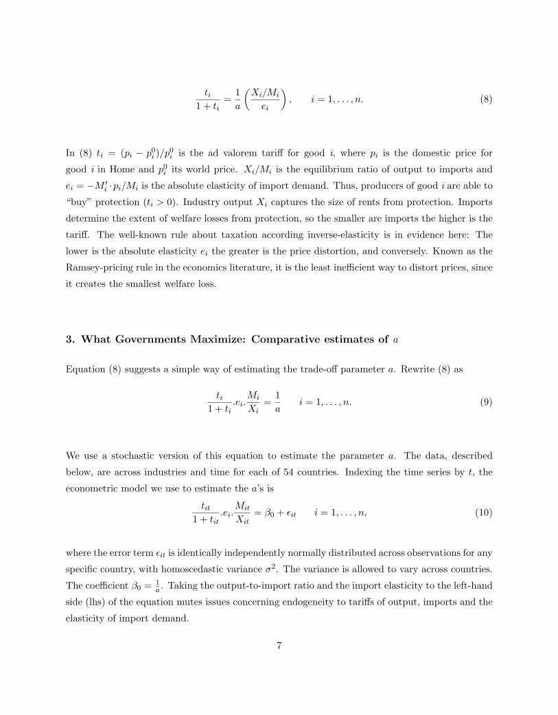
ti1 + ti

=1a

(Xi/Mi

ei

), i = 1, . . . , n. (8)

In (8) ti = (pi − p0i )/p0

i is the ad valorem tariff for good i, where pi is the domestic price for

good i in Home and p0i its world price. Xi/Mi is the equilibrium ratio of output to imports and

ei = −M ′i ·pi/Mi is the absolute elasticity of import demand. Thus, producers of good i are able to

“buy” protection (ti > 0). Industry output Xi captures the size of rents from protection. Imports

determine the extent of welfare losses from protection, so the smaller are imports the higher is the

tariff. The well-known rule about taxation according inverse-elasticity is in evidence here: The

lower is the absolute elasticity ei the greater is the price distortion, and conversely. Known as the

Ramsey-pricing rule in the economics literature, it is the least inefficient way to distort prices, since

it creates the smallest welfare loss.

3. What Governments Maximize: Comparative estimates of a

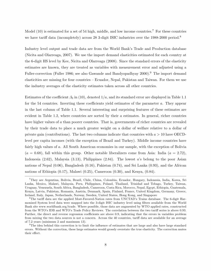
Equation (8) suggests a simple way of estimating the trade-off parameter a. Rewrite (8) as

ti1 + ti

.ei.Mi

Xi=

1a

i = 1, . . . , n. (9)

We use a stochastic version of this equation to estimate the parameter a. The data, described

below, are across industries and time for each of 54 countries. Indexing the time series by t, the

econometric model we use to estimate the a’s is

tit1 + tit

.ei.Mit

Xit= β0 + εit i = 1, . . . , n, (10)

where the error term εit is identically independently normally distributed across observations for any

specific country, with homoscedastic variance σ2. The variance is allowed to vary across countries.

The coefficient β0 = 1a . Taking the output-to-import ratio and the import elasticity to the left-hand

side (lhs) of the equation mutes issues concerning endogeneity to tariffs of output, imports and the

elasticity of import demand.

7

Model (10) is estimated for a set of 54 high, middle, and low income countries.7 For these countries

we have tariff data (incompletely) across 28 3-digit ISIC industries over the 1988-2000 period.8

Industry level output and trade data are from the World Bank’s Trade and Production database

(Nicita and Olarreaga, 2007). We use the import demand elasticities estimated for each country at

the 6-digit HS level by Kee, Nicita and Olarreaga (2008). Since the standard errors of the elasticity

estimates are known, they are treated as variables with measurement error and adjusted using a

Fuller-correction (Fuller 1986; see also Gawande and Bandyopadhyay 2000).9 The import demand

elasticities are missing for four countries – Ecuador, Nepal, Pakistan and Taiwan. For them we use

the industry averages of the elasticity estimates taken across all other countries.

Estimates of the coefficient β0 in (10), denoted 1/a, and its standard error are displayed in Table 1.1

for the 54 countries. Inverting these coefficients yield estimates of the parameter a. They appear

in the last column of Table 1.1. Several interesting and surprising features of these estimates are

evident in Table 1.2, where countries are sorted by their a estimates. In general, richer countries

have higher values of a than poorer countries. That is, governments of richer countries are revealed

by their trade data to place a much greater weight on a dollar of welfare relative to a dollar of

private gain (contributions). The last two columns indicate that countries with a > 10 have OECD-

level per capita incomes (with the exception of Brazil and Turkey). Middle income countries have

fairly high values of a. All South American economies in our sample, with the exception of Bolivia

(a = 0.68), fall within this group. Other notable liberalizers come from Asia: India (a = 2.72),

Indonesia (2.62), Malaysia (3.13), Philippines (2.84). The lowest a’s belong to the poor Asian

nations of Nepal (0.06), Bangladesh (0.16), Pakistan (0.74), and Sri Lanka (0.93), and the African

nations of Ethiopia (0.17), Malawi (0.25), Cameroon (0.30), and Kenya, (0.84).

7They are Argentina, Bolivia, Brazil, Chile, China, Colombia, Ecuador, Hungary, Indonesia, India, Korea, SriLanka, Mexico, Malawi, Malaysia, Peru, Philippines, Poland, Thailand, Trinidad and Tobago, Turkey, Taiwan,Uruguay, Venezuela, South Africa, Bangladesh, Cameroon, Costa Rica, Morocco, Nepal, Egypt, Ethiopia, Guatemala,Kenya, Latvia, Pakistan, Romania, Austria, Denmark, Spain, Finland, France, United Kingdom, Germany, Greece,Ireland, Italy, Japan, Netherlands, Norway, Sweden, United States, Hong Kong, and Singapore

8The tariff data are the applied Most-Favored-Nation rates from UNCTAD’s Trains database. The 6-digit Har-monized System level data were mapped into the 3-digit ISIC industry level using filters available from the WorldBank site www.worldbank.org/trade. Where possible, those data are augmented by WTO applied rates, constructedfrom the WTO’s IDB and WTO’s Trade Policy Reviews. The correlation between the two tariff series is above 0.93.Further, the direct and reverse regression coefficients are above 0.9, indicating that the errors in variables problemfrom mixing the two data sources is not a concern. Across the 40 countries, tariff data are available for an averageof 7.2 years (minimum 2 and maximum 13).

9The idea behind this correction is to limit the influence of estimates that are large and also have large standarderrors. Without the correction, these large estimates would grossly overstate the true elasticity. The correction mutestheir effect.

8

An important feature of our results is that, in contrast with previous examinations of the Grossman-

Helpman model (Goldberg and Maggi 1999, Gawande and Bandyopadhyay 2000, Mitra et al. 2002,

McCalman 2004, Eicher and Osang 2002), our estimates of a are reasonable, both qualitatively

(poorer countries have smaller a’s than richer countries) and quantitatively (only extremely low-

tariff or zero-tariff countries like Hong Kong and Singapore have a’s greater than 50, while this

was routinely found for Turkey, Australia, and the U.S. in the studies referenced above). We find

the cross-country variation in a to be striking and intuitively pleasing. Countries with low a’s

accord with the widely accepted view that governments in those countries are also among the most

corrupt in the world. Indeed the Spearman rank correlation between Transparency International

Perception Corruption Index for the year 2005 and our measure of government willingness to trade

off social welfare for political rents is 0.67, and we can statistically reject the assumption that

the two series are uncorrelated. In 2005 the Transparency International Corruption index rank

of the two countries at the bottom of our a rankings (Nepal and Bangladesh) were 121 and 156

out of 157 countries, respectively. Similarly, the Transparency International Corruption index rank

of the two countries at the top of our a rankings (Singapore and Taiwan) were 5 and 15, respectively.

Some results we find to be surprising are (i) the low a for Mexico, despite it’s membership in

NAFTA, (ii) the lower than expected a for the OECD countries of Norway, Ireland and the Nether-

lands (in the 3 < a ≤ 5 group), (iii) the relatively high a’s for the socialist countries in transition,

including Poland, Hungary and Romania, (iv) the relatively high a’s for Japan and China, both of

whom have been criticized for being mercantilistic – protectionist and export-oriented.

These unexpected results emphasize the fact that the theoretical model does not base it’s prediction

simply on openness (low or high tariffs), but also the import-penetration ratio, and import demand

elasticities, as well as their covariance with tariffs, and each other. The incidence of tariffs in

industries with high import demand elasticities reveals the willingness on the part of governments

to (relatively) easily trade public welfare for private gain,10 since in welfare-oriented countries the

most price-sensitive goods should be distorted the least. The incidence of tariffs in industries

with high import-to-output ratios also reveals the willingness on the part of those governments

to trade public welfare for private gain since distorting prices in high-import sectors creates large

deadweight losses. Empirically, this is not only revealed by the surprising estimates discussed above,

but also by the relatively low correlation between our estimates of a, and average tariffs, which is

10This results in a high estimate of β0 and low estimates of a.

9

estimated at 0.33, and compares badly with the correlation with the index of perceived corruption.

Thus, the estimates underscore the need to consider more than simplistic measures of openness in

order to make inferences about the terms at which different governments trade public welfare for

private gain. The Grossman-Helpman measure is not only theoretically more appropriate, but also

empirically it appears to be quite distinct from simpler measures.

We are ultimately interested in the deeper question of why governments behave as they do. What

explains the variation in the estimates of a across countries? Why do some countries have low a’s

and others high a’s? Are polities in poorer countries content to let their governments cheaply trade

their welfare away? If so, why? And why in richer countries do we observe the opposite? These

are the questions to which we devote the remainder of the paper.

4. Explaining the variation in a: Theory

To explain why a varies across countries we delve into institutional foundations of policymaking. In

this, we can take one of two routes. One is a data-driven approach that involves choosing a set of

variables that adequately describe institutional details of the policy process in different countries,

and use them to econometrically explain the cross-country variation in a. Such a method would

shed light on those institutions that motivate governments to behave as they do in setting trade

policy. The second is to seek structural explanations of how institutions might explain the variation

in a across countries. We opt for the latter in this paper, since it continues in the tradition of the

Grossman-Helpman (1994) model that delivered our estimates for a.11

Positive theories that model policy outcomes based on institutional details of the policy process fall

into three broad categories (Helpman and Persson 2001). Electoral competition models focus on the

process by which parties are represented in the legislature, and feature details about the structure

of voter characteristics (informed versus uninformed) and voter preferences. Lobbying models focus

on lobbying process and feature details about the lobbying game. Legislative bargaining models

feature specific legislative decision making processes that may emphasize, for example, agenda-

setting and the allocation of policy jurisdictions (e.g. ministers, committee chairs). In the first

part of this paper we used the GH94 lobbying model to estimate the weight put on social welfare

11We have also followed the data-driven approach using factor-analytic methods. The factor analysis approachyields results that reinforce many of the findings in this paper. The results are available to interested readers uponrequest.

10

from trade policies of governments. But the determinants of these weights were a “black box”. The

objective of this section is to unravel the determinants of a as viewed from the theoretical lens of

electoral competition and legislative bargaining models.

4.1 Electoral Competition and lobbying

Integrating lobbying and electoral competition has been done in three important models: Austen-

Smith (1987), Baron (1994), and Grossman and Helpman (1996). They model policies as outcomes

from the interaction of two parties and special interest groups that make lobbying contributions

to them. They differ in the motives of the lobbyists. Lobbyists are purely interested in altering

electoral outcomes in Austen-Smith and Baron. In Grossman and Helpman, lobbyists are also able

to influence policy outcomes by altering party platforms via lobbying. We will abstract from the

electoral motive and focus on this influence-seeking motive in order to connect the a parameter

with more primitive institutional details. To this end, we describe the 1996 Grossman-Helpman

(henceforth GH96) model.

Two parties, A and B, contest an election for seats in the legislature. Each party advances a slate

of candidates, and the country votes as a single constituency. Once elections are over, and the votes

counted, both parties occupy seats in legislature in proportion to the popular vote count (more on

the distinction between this proportional system and a pluralitarian system below).

There are two classes of voters, informed and uninformed. The former have immovable preferences

based on (i) the policy position of each party and (ii) other characteristics of the party (liberal,

conservative). Uninformed voters, on the other hand, may be induced to move from their cur-

rent position via campaign expenditures on slogans, advertising, and other informational devices

designed to impress them. The difference in campaign spending by the two parties crucially de-

termines how many uninformed voters they will be able to move to their side. For this reason,

politicians representing each party demand contributions. Lobbies form to supply contributions.

On the lobbying side we consider the case, as in the GH94 model, where each sector is represented

by a single lobby, but the fraction of the organized population represents a negligible proportion

of the total population. Each lobby is interested only in protecting its own sector, and there is

no competition or conflict among lobbies.12 Each party thus receives contributions from multiple

12This exemplifies Baron’s (1994) idea of “particularistic policy” whose benefits are exclusively enjoyed by those

11

lobbies, with each lobby’s interest being a single element of the vector p. The game comprises of

two stages. In the first stage, lobbies announce their contribution schedules (as a function of the

tariff afforded to their sector), one to each of the two parties (party A and party B). In the second

stage, the two parties choose their vector of tariffs (their policy platforms) in order to maximize the

representation of their party in the legislature. The lobbies then pay their promised contributions,

the parties wage their campaigns, and the legislature/congress that assumes office implements one

of the party’s tariff vector (legislative processes are a black box in electoral competition models –

we unpack this box below).

A political microfoundation for a is found in the structural analog of the expression for the joint

surplus in (5), which we replicate here.

Ωi = Wi(ti) + aW (ti), i = 1, . . . , n. (11)

In the GH94 unitary government case, the politically optimal tariffs in each sector i is set by the

government in a way that maximizes the weighted sum of the aggregate welfare of lobby i and the

aggregate welfare of the country’s citizens. The government is induced by lobby i to weight the

lobby’s interest by (1+a), which is greater than the weight of a it places on the public’s aggregate

interest. We will observe a parallel between (11) and the joint surplus in the electoral competition

game, and use it to pin down the determinants of a from the parameters of the electoral competition

game.

GH96 (p. 274 eq. (4)) show that the joint surplus in the electoral competition game involving

parties A and B and one (say, sector i) lobby is

ΩKi = φKWi(ti) +

1− α

α

f

hW (ti), K = A,B. (12)

As in (11), Wi(ti) is the (net of contributions) welfare of lobby i. In (12) W (ti) is the aggregate

welfare of informed voters. There are four parameters to consider. α is the fraction of voters who

who lobby for it, but the costs are not onerous on others. Note that this assumption allows us to use the GH96single-lobby results, since lobbies do not compete with each other for political favors.

12

are uninformed. If α = 0, then W (ti) becomes the welfare of the average voter, just as in (11).

We will see below that buying the support of uninformed voters makes special interests groups

important to political candidates, and α determines the magnitude of the importance of special

interest contributions. f > 0 quantifies the diversity of views about the two parties among voters

in terms of all fundamental characteristics (e.g. liberal-conservative) except their policy positions

about the tariff ti. The closer is f to zero the greater is the diversity of views; the larger is

f the closer are the two parties perceived to be. This parameter is relevant because the more

important these divergences among the parties are to voters - the more committed they are to a

particular party for ideological reasons, for example – the less likely they are to be swayed by trade

policy. h > 0 quantifies the ability of campaign spending to move the position of an uninformed

voter. The greater is h, the more productive is a dollar of campaign spending in influencing the

uninformed voter. Since money becomes a useful instrument with which to sway the uninformed

voter, the sources of this money – special interest groups – become useful to the political candidates.

Finally, φK is the probability that, once elections are over, the legislature actually adopts party

K’s trade policy platform (sector i tariff promised by party K before the election). With two

parties, φA +φB = 1. We will see below the relevance of this key parameter in formulating testable

hypoteses.

The parallel with (11) is clear. (12) shows that each party is induced by lobby i to maximize a

weighted sum of the aggregate interest of informed voters and the aggregate interest of members

of organized interest groups. The aggregate interest of informed voters (interest groups) receives

a weight that increases (decreases) with the share of informed voters in the population (1 − α),

decreases (increases) with the diversity of their views about the parties’ ideological positions, and

decreases (increases) with how easily uninformed voters are swayed by campaign spending. We will

use these and other observations to make empirically testable predictions.

Predictions

Proportional vs. Pluralitarian systems

In a proportional system seats in the legislature are allocated to the two parties according to the pro-

portion of the popular vote. With just two parties, and the country voting as a single constituency,

the objective of maximizing the number of seats in legislature is equivalent to maximizing plurality.

That is, the outcome is exactly the same as if the system of representation were majoritarian. The

13

GH96 model is such a 2-party one-constituency model. The real world is different in two important

respects.

First, a country typically votes not as a single constituency, but as several geographically distinct

constituencies. In a typical majoritarian system each district elects a single representative to the

legislature. In a typical proportional system each district is represented by multiple candidates

so that a district’s seats are divided between the two parties in proportion to the popular vote.

If districts are heterogeneous, say, with respect to the composition of specific factors, then it is

possible for a majoritarian system to favor special interests more than a proportional system. This

is demonstrated theoretically in Grossman and Helpman (2005). They advance a 2-party 3-good,

3-district model in which the districts are heterogeneous in the composition of (three) specific

factors. There are no lobbies, however, each legislator seeks to represent the interests of their

average constituent. Grossman and Helpman (2005) show that if both parties seek a majority13 in

the legislature then, because the election of legislators is tied to particular geographic or economic

interests, there is greater protection than if legislators’ interests were more closely tied to the

national, not regional, interests.

Consider the 2-party 3-district example under a system of proportional representation in which

candidates from both parties compete for multiple seats within the same district. Evans (2008)

shows that it is more likely in the case of proportional representation that one party sweeps the

election, that is, wins a majority in all three districts, than under a majoritarian system (in which

the single seat per district is determined by majority vote in each district). If one party sweeps the

election, the policy it chooses reflects national, not regional, interests, that is, free trade (Grossman

and Helpman 2005, eq. (4)). Thus, a majoritarian system of representation leads to greater

protection than a proportional one.14

This result does not require the presence of lobbies because the model is devoid of uninformed

voters. If lobbies were admitted, what does this result imply about the distribution of a across the

two systems of political representation? We surmise that since a majoritarian system is predisposed

to being protectionist (it has a lower probability of sweeping the states than a proportional one),

13This objective is different from maximizing the number of seats as in GH96.14Rogowski’s (1987 p. 208) prescient logic argued that since proportional systems makes states more independent

from rent-seekers than majoritarian systems, the former leads to more stable and long-lived political commitmentsto free trade than the latter. The reason for this is that proportionate systems result is stronger (and fewer) partiesthan majoritarian systems.

14

lobbies will ensure their interests are weighed more heavily in (12) in majoritarian systems than in

proportional ones. That is, all else constant, a’s are lower in proportional than in a majoritarian

systems. A formal demonstration of this requires extending the GH96 single-district electoral

competition model with uninformed voters (whose presence motivates the existence of lobbies) to

n districts.15 We state our first hypothesis as:

Hypothesis 1: A majoritarian system favors special interests more than does a proportional

system. Majoritarian systems are therefore associated with low a’s.

It is possible that the 3-district example exaggerates the predisposition of proportional systems to

be less protectionist than majoritarian ones, so that as the number of districts increases the prob-

ability of sweeping the districts becomes more remote and the distinction between the two systems

disappears. A rejection of Hypothesis 1 would then indicate that the world is well approximated

by the GH96 2-party single-district model in which proportional representation is equivalent to

plurality.

The second difference between the GH96 construct and the real world is that democracies typically

have more than two parties. In the data section we attempt to reconcile the two-party theoretical

model with multi-party governments that we find in the data.

Uninformed voters

Consider the fraction α of uninformed voters. A comparison of the weights on W in (11) and (12)

indicates that, all else held constant, a → 0 as α → 1. The intuition for this result is this. In the

absence of lobbying, parties will chose their platform to attract the maximum number of informed

voters. Denote this tariff as t∗i . To persuade party A to adopt a tariff ti, lobby i must contribute an

amount that delivers at least as many uninformed votes as would t∗i .16 The larger is the proportion

of uninformed voters α, the more pivotal the uninformed voter becomes. Since the resources for

launching a campaign to sway uninformed voters are provided by lobby i, the lobby’s welfare (here

profits) gets greater weight in (12). This leads to our second prediction:

Hypothesis 2: The larger is the proportion of uninformed voters in the population, the lower is

a, and conversely.

15This exercise is outside the scope of this paper and left open for future research.16GH96 (p.274) show that this is amount equals 1−α

αfh[W (t∗i )−W (ti)].

15

Given the cross-country distribution of a, testing this hypothesis amounts to testing the validity of

the uninformed voter construct itself. The existence of uninformed voters is central to the GH96

model since it motivates the existence of lobbies. It is also central to a number of models that

feature Baron’s idea of the uniformed voter.

Party Ideology

Consider the ideological divide between the two parties given by parameter f . The larger is f ,

the smaller is the diversity of views among voters over the fundamental characteristics of the two

parties. A comparison of the weights on W in (11) and (12) indicates that, all else held constant,

a → 0 as f → 0. The reason why the weight put on social welfare increases as f increases is this.

With little diversity of views among voters, a tariff that deviates from that favored by the average

voter does great damage electorally. When there is great diversity of views and the two parties are

considered to be very dissimilar, the parties can afford to set (district i’s) tariff different from t∗i

and still retain the favor of voters who were inclined to vote for them on the basis of, say, ideology.

In contrast, if voters are indifferent between the two parties’ basic characteristics, a policy that

deviates from t∗i risks losing many voters to the other party. This leads to our third prediction:

Hypothesis 3: The greater is the perceived difference in the fundamental characteristics of the

two parties in the eyes of voters, the lower is a, and conversely.

In sum, if voters are clearly predisposed to one party or the other on the basis of attributes other

than their policy platforms, then both parties are more cheaply able to impose welfare costs on

the public. The parties will calculate that they gain more uninformed voters than lose the votes of

their supporters.17

Susceptibility of the Uninformed Voter

Finally, consider the productivity of campaign spending parameter h. A comparison of the weights

on W in (11) and (12) indicates that, all else held constant, a → 0 as h → ∞. With greater

power of the dollar to influence uninformed voters, it is less costly to deviate from t∗i . Hence, as

h increases, both parties are induced to place greater weight on the interest of lobby i than on

17Hypothesis 3 may be extended in future research more generally to the extent of not just political but othersources of polarization, for example economic inequality, or separate cultural/tribal identities, thus connecting thehypothesis about the determinants of a to the voluminous literature on sources of polarization.

16

the interest of the informed public. This leads to our fourth and last prediction from the electoral

competition model:

Hypothesis 4: The greater is the ability of a dollar of campaign spending to influence uninformed

voters, the lower is a, and conversely.

We now turn to the interactions among legislators and the process by which decisions are made

within legislatures.

4.2 Legislative Bargaining and lobbying

The Baron-Ferejohn (1989) model is the proven workhorse in the area of legislative bargaining.

Models of legislative decision-making have had to struggle with Arrow’s (1963) result that it is

not possible to select the best action from a set of alternatives according to some voting rule (e.g.

majority wins). The breakthrough has been the introduction of an agenda setter who is granted

institutional power to champion a specific alternative and who attempts to guide voting in the

direction of that agenda. Regardless of whether that agenda is selected over the status quo, a

voting equilibrium exists.18

We adapt Persson’s (1998) legislative bargaining model of public goods provision with lobbying to

search for more hypotheses about the determinants of a. An attractive feature of the legislative

bargaining model is that it allows us to link a with asymmetric powers of legislators. Specifically, it

motivates the role of checks and balances on those powers, without which there would be extreme

redistribution.

To make our point simply, consider legislation of a slate of tariffs ti, i = 1, . . . , n. Assume that

sectors are regionally concentrated – in each of the n districts is located one sector. Every district

sends one representative to the legislature. However, there is an exogenous institutional constraint

on the amount of protection: the welfare loss from the set of tariffs/subsidies may not exceed a

prespecified amount. This constraint may be satisfied by limiting the number of sectors that receive

protection, or limiting the level of tariffs/subsidies, or both. The existence of such a constraint is

18Determining the set of alternatives from which the agenda setter selects forms the literature on “agenda forma-tion” (e.g. Baron and Ferejohn 1987b). We will abstract from those issues and presume the agenda setter’s agendais admissible in the legislature.

17

motivated below. Each legislator maximizes an objective function that is the sum of the welfare

of the constituents in her district and the rents obtained from tariff policy.19 That is, a legislator

cares specially about the rents from the tariff to her sector, over and above other components of

welfare. There are two reasons for this assumption. One is that it is consistent with the existence

of lobbies that pay the legislators for producing these rents. The other is votes: the electoral

competition model in which the money is used to get uniformed voters to vote for the legislator

may be embedded here.

First, consider how the legislature sets the tariff vector when there are no lobbies. The legislative

bargaining game follows a typical sequence of events: (1) A legislator is chosen to be an agenda

setter S. (2) She makes a policy proposal for adopting the vector tSi . (3) The legislature votes

on the proposal, and if it gets simple majority tSi is implemented. Otherwise, the status quo

outcome, say toi , is implemented. The agenda setter is obviously interested in using her powers

to benefit her district, but must obtain a majority that goes along with her tariff agenda tSi .She must therefore guarantee at least the same payoff to the legislators she courts as they would

receive under the status quo.20 Persson shows that the agenda setter will set an agenda that forms a

minimum winning coalition composed of a simple majority such that (i) legislators (sectors) outside

of the winning coalition get no tariffs/subsidy even though they bear part of the welfare loss, (ii)

the members of the winning coalition get just enough protection/subsidy that they are not worse

off than in the status quo.21

The logic behind this stark, rather pessimistic, result is that intense competition among legislators

to be part of the winning coalition enables the agenda setter to dictate terms. This competition

drives down the “price” (or weakens the terms) a legislator can charge the agenda setter. The agenda

setter uses her powers to provide the highest rents possible to her district, since the competition

among legislators endows her with bargaining power.

The same logic drives the results when we introduce lobbying into the game. Suppose every sector

(district) has an organized lobby that makes contributions to their legislator. Their fierce desire to

have their legislator be part of the winning coalition cedes any bargaining ability they may have to

19In Persson’s model legislators may each attach different weights. We presume all legislators attach the samepositive weight.

20In the presence of the welfare loss constraint, she must sacrifice some rents that would have otherwise gone toher district in order to form a coalition of legislators that would implement her agenda. More on this below.

21If the weights on rents are heterogeneous across legislators, then a third condition applies: (iii) the members ofthe winning coalition are those that have the highest weights – that is, they are the cheapest to buy off.

18

the agenda setter. Their contributions are unable to move the agenda in their favor. An interesting

result in the lobbying game is that since no sector outside the district of the agenda setter receives

any protection/subsidy, they contribute close to zero.22

Checks and Balances

Checks against the agenda setter’s powers may be placed by an individual with influence over policy

at the national level, say, a president. His policy platform consists of a specific limits on welfare

losses from price distortions. Our exogenously specified limit on welfare loss is thus motivated as

a way of instituting checks and balances. Once again, the same conclusion applies – competition

among legislators still enables the agenda setter to get away with what rents are possible. The

difference is that the rents are lower, if the elected president’s platform is more limiting than the

status quo.23

Clearly, a direct way of enhancing the bargaining power of legislators other than the agenda setter,

and thus checking her powers, is via a binding limit on the rents the agenda setter can direct to

her district. Such a national policy would then allow the legislative bargaining game to allocate

rents to other districts. Regardless, both types of Presidential platforms – limits on the amount of

total welfare loss, or limits to the rents accruing to the agenda setter’s district – will result in a

lower redistribution compared with a legislature that does not allow representation of a nationwide

polity capable of checking legislators. We state the first hypothesis from the legislative bargaining

game.24

Hypothesis 5: Executive checks will limit the ability of legislators to impose their politically

optimal welfare losses. Greater checks are therefore associated with higher values of a.

Our final two hypotheses go beyond the existing literature, and feature electoral competition for

22The model may be extended to incorporate the two-party electoral competition model in determining the legislatorchosen to represent a district. Then, the diversity across districts in the parameters α, h, f , and φ then underlies eachlegislator’s a parameter. This may well determine which legislators are in the winning coalition (that is, which arethe cheapest for the agenda setter to buy off), but the fact still remains that competition among legislators will leadto the same policy.

23Persson, Roland and Tabellini (1997) give deeper meaning to what it means for the executive to wield checks andbalances. Their mechanism is separation of powers. Further, separation of powers works to produce welfare-orientedoutcomes only if no policy can be implemented unilaterally, i.e., without the consent of both bodies. Otherwise, therewould be excessive (unilateral) claims on government resources at the expense of voters.

24The legislative bargaining game has an additional step: (1) The executive chooses a limit on the total welfareloss (or the rents to the agenda setter’s district). The other three steps follow as before.

19

the executive. An unsatisfactory aspect of legislative bargaining theory is its presumption that

the executive represents median voter interests. In most real-world democracies the executive

is elected and lobbied. We therefore embed the two-party electoral competition game into the

legislative bargaining model.

Electoral Competition for the Executive

Two candidates, representing parties A and B respectively, contest the Presidential election. The

structure of the game is essentially similar to the game used to model electoral competition for

legislative seats. The main difference here is that the presidential platforms concern not the tariff

directly but limits on the total welfare loss from trade protection denoted L. The executive is

presumed to maximize an objective function like (4), except that the argument is L (the set of

tariffs t are determined conditional on L, see (13) below). When there are no lobbies, the executive

seeks to maximizes national welfare and sets L = 0 eliminating the possibility of any tariff or

subsidy. Lobbies representing import-competing producers attempt to move L away from zero so

that they might benefit from tariffs, conditional on L, that are decided in the legislative bargaining

process.

The cap on welfare loss, L, is determined as the outcome of the two-party election in which a national

polity of informed and uninformed voters participate. Thus, L for each of the two Presidential

candidates is determined as the Nash bargaining solution to25

MaxL ΩKP = φK

P

∑i

Wi(L) +1− α

α

f

hW (L), K = A,B, (13)

where Wi(L) is the (net of contributions) welfare of the lobby from district i and W (L) is the welfare

of the average informed voter, α is the fraction of uninformed voters, f quantifies the diversity of

views about the two parties among voters, and h is productivity of campaign spending. φP is the

probability that, once elected, the president is able to get the legislature to adopt L.

The first result follows directly from (13). The parameter φKP – the probability of successfully

legislating candidate K’s executive platform – determines the weight that special interests get in

the executive electoral competition game. If φKP is non-negative then the first term on the right-

25The logic behind (13) is similar to the logic behind (12) in the legislative electoral competition game.

20

hand side of (13) indicates that L is selected to be greater than zero by both candidates. Thus,

electoral competition with lobbies and uninformed voters induces both candidates to impose welfare

loss on the national polity. The parameters α, h, f work to change a in the same direction when

there is electoral competition for the executive as they did with electoral competition for seats in

legislature. We state this hypothesis as the next hypothesis.

Hypothesis 6: Electoral competition for the executive is associated with lower values of a than if

there were no electoral competition for the executive.

Importantly, the parameter φKP determines the executive’s ability to impose checks on legislature’s

powers. When government is undivided, that is, when the executive and legislature both belong

to the same party, the executive’s platform is more likely to make it past the legislature than were

government divided (see e.g. Elgie 2001). Thus, (13) implies that the higher is φKP (undivided

government), the more the executive platform of candidate K is bent to satisfying special interests

at the expense of the public. Conversely, if φKP is low (divided government), the executive is a more

effective check on the legislature’s ability to impose welfare costs on the public.26 We state this as

our final hypothesis.27

26An opposite argument is advanced in Lohmann and OHallorans (1994). In their model a divided government doesnot delegate policymaking powers to the president, while a government with a clear majority in Congress does. Thus,under divided government trade policy should be more protectionist. The reason is that each legislator cares aboutprivate benefits and costs of protection to their own district and not the social costs. The social cost that individuallegislators impose in a divided Congress that is trapped into distributive logrolling, leads to inefficiently high levels ofprotection. Further, under divided government, the presidents discretionary powers are more constrained thereforeassociating divided governments with higher levels of protection and majority government with freer trade.

27The legislative bargaining theory may completed as follows: In the agenda setter’s district, two candidatescompete to become the agenda setter. Their platforms, consisting of the tariff for their district tS (conditional onthe executive’s limit on welfare loss that may be nationally imposed by trade policy L) that they propose to pushthrough the legislature, are determined as the Nash bargaining solution to

MaxtS ΩKS = φK

S WS(tS(L)) +1− α

α

f

hW (tS(L)), K = A, B. (14)

WS(tS(L)) is the welfare of the district S lobby, W (tS(L)) is the welfare of the average informed voter in district S,and α, f, h are the same as the national-level parameters. φS is the probability that, once elected, the agenda setteris able to get the legislature to adopt tS . Since φS determines how much weight special interests get in the electoralcompetition game in the agenda setter’s district, it may be used to establishing a relationship between executivechecks and a. In (13) φS is a function of the ceiling on the welfare loss L, and if the constraint is binding, is smallerthan if there were no national-level check on the agenda setter’s powers. Thus, φS(L) ≤ φS(L = inf). We can usethis result to develop hypotheses about the agenda setter, but that would be largely theoretical exercise. Identifyingagenda setters across our sample of countries is beyond the scope of our data. We leave this as an open comparativepolitical economy question deserving further work.

21

Hypothesis 7: Divided government leads to higher values of a than if the party of the executive

were the same as the majority party in the legislature.

5. Explaining the variation in a: Data and Results

5.1: Data

Recent interest in the influence of institutions over economic and political outcomes has led to the

creation of cross-country databases of political institution. We draw on the high-quality Database

on Political Institutions (DPI) constructed by Beck et al. (2001). The database contains a number

of variables measuring the nature of “government”, “legislatures”, “executive”, and “federalism”.

They are measured both, qualitatively and quantitatively, and admirably serve our purpose of

measuring the variables required to test the hypotheses. We also use economic data from various

issues of the World Development Indicators (WDI). Media cost data are from World Advertising

Trends (1998).

The theory upon which we base the empirical investigation requires us to consider only democra-

cies.28 We rely on the variable LIEC (Legislative Index of Electoral Competitiveness) in the DPI

database to identify democracies. LIEC scores vary between 1 (no legislature) and 7(largest party

received less than 75% of the seats). Lower scores are given to unelected legislatures (score=2) or

if the legislature is elected but comprises just one candidate (score=3) or just one party (score=4).

Countries with scores of 4 or less are not considered to have legislatures featuring electoral com-

petition. Only countries in which multiple parties contested for seats in the legislature (scores of 5

or more) are considered in the sample. Among the 54 countries for which we have estimated the

parameter a, only four are dropped on this count (China, Hong Kong, Ethiopia, Taiwan).29

28A recent literature has argued in favor of democracies on the broader issue of whether democracies producebetter trade policy outcomes than non-democracies. Milner and Kubota (2005) argue that democratization reducesthe ability of governments to use trade barriers as a strategy for gaining political support. The reason is thatdemocratization implies a movement towards majority rule rather than leaders representing small groups. Usingan elegant and simple trade model they show that the optimal level of protectionism declines with the size of thewinning coalition. Mansfield, Milner and Rosendorff (2000 and 2002) also argue that democracies are more likelyto adopt trade policies that reflect voters interests rather than the interest of a small group of pressure groups, butfor a different reasons. In a world with asymmetric information where voters cannot distinguish perfectly betweeneconomic shocks (over which leaders have little control) and deliberate extractive policies, trade agreements aidleaders in signaling their actions to home voters, since their partners in the trade agreement will hold them up totheir actions.

29Taiwan had an LIEC score of 2 during the early 1990s, the period from which we used data to estimate its a.

22

Testing Hypothesis 1, requires identifying legislatures elected using a proportional system of rep-

resentation – where seats are allocated on the basis of the proportion of votes received – versus a

pluralitarian first-past-the-post systems.30 The variable HOUSESYS in the DPI is used to iden-

tify countries with proportional versus pluralitarian systems. HOUSESYS is coded 1 in the DPI

only if the majority of the house is elected on a plurality basis. We define the binary variable

PROPORTIONALITY=1-HOUSESYS to indicate legislatures in which parties are (largely) repre-

sented proportionally to the votes they receive.31

We must reconcile the theoretical model, which admits only two parties, with the presence in

our data of many countries with multi-party governments. How the probability of successfully

legislating the platform of the party in power changes when there are more than two parties is

the main question must be addressed. The greater this probability (i.e. large φK), the greater

the weight given to special interests in (12), and the lower is a. In a government comprising more

than one party and/or an opposition that also comprises a coalition of parties, the probability of

successfully legislating the winning party’s platform hinges on party concentration and cohesiveness

(see e.g. McGillivray 1997). Further, Powell and Whitten (1993) have argued that retrospective

economic voting (giving the government credit or blame for economic outcomes) will be more likely,

the easier it is for voters to attribute economic outcomes to a particular party or coalition. So more

cohesive coalitions have greater incentives to use economic policies for political purposes, while

looser ones have fewer incentives.32

We extend the hypothesis about proportionate versus majoritarian systems by interacting PRO-

PORTIONAL and (1-PROPORTIONAL) with Herfindahl indices of party concentration in the

30The influence of proportional versus other systems of electing legislatures has been well-researched in the contextof protection. Mansfield and Busch (1995) found that during the 1980s countries with proportional systems had highernontariff barriers than countries with majoritarian system. Willmann (2005) suggests that this might be so becausea districts in majoritarian systems select more protectionist representatives than their median voters. Hatfield andHaulk (2004) show the opposite – that during 1980-2000, Latin American and OECD countries with proportionalsystems had lower tariffs than countries with majoritarian system. Evans (2008) affirms this finding using data fornearly 150 countries during 1981-2004.

31The DPI contains the variable PR that takes the value 1 if any candidates are elected based on the proportionof votes received by their party and 0 otherwise. Even a small fraction the legislature is elected using both, then PRis coded 1. Another variable PLURALITY does similarly for pluralitarian systems. A problem with using either ofthese measures is that a number of countries have PR=PLURALITY=1, indicating the presence of both systems.Coding according to HOUSESYS is cleaner and leads to a measure that is either proportional or pluralitarian, butnot both.

32In order to admit more than 2 parties, we assume that each party uses its platform to seeks absolute majority inthe legislature. The platform may not be bent to “buy in” coalition partners ex ante. The largest winning party’splatform may be bent after the coalition forms in legislature, but the platform eventually supported is closer to thewinning party than the platform of the (largest party in the) opposition.

23

government (HERFGOV) and opposition (HERFOPP). We define the difference GOVCOHESION

= HERFGOV - HERFOPP to measure party cohesion in the government relative to the opposition.

The greater is HERFDIFF, the more cohesive is the government coalition; the smaller is HERFD-

IFF, the more fractured the government and/or the more united the opposition. We use the two in-

teractions, PROP+GOVCOHESION = PROPORTIONAL×HERFDIFF and PLUR+GOVCOHESION

= (1-PROPORTIONAL) × HERFDIFF, to test the idea that plurality plus party cohesion in gov-

ernment (relative to the opposition) leads to greater success in legislative voting than proportion-

ality plus party cohesion within the government.

Hypothesis 1.2: A majoritarian system with cohesion among parties in power favors special

interests more (i.e. have lower a’s) than does a proportional system with the same party cohesion.

At the heart of electoral competition models with lobbying is the fraction α of uninformed voters.

We capture two different dimensions of what it means for voters to be “uninformed”. In the GH96

model (and the Baron model upon which it is based) uninformed voters are impressionable voters

who do not know the policy positions of candidates. We capture the idea of uninformed voters as

impressionable voters using two variables. The first variable is the proportion of the population that

is illiterate (ILLITERACY), which directly measures that part of the population whose opinions

are more vulnerable to campaign spending. There is some evidence that lower literacy is associated

with being uninformed politically, even in developed countries. A primary survey by Blais et al.

(2000, Table 1) of Canadian voters indicated that high school dropouts indicated not knowing

about a large proportion of high-profile political candidates, relative to those who had completed

university. In developing countries this problem is worse. Bardhan and Mookherjee (2000) add

that political capture by lobbies in developing countries is (i) decreasing in the average level of

political awareness, and (ii) increasing in the awareness disparity across economic classes. These,

in turn are correlated with illiteracy and poverty.

The second variable is the proportion of the population that is urbanized (URBANIZATION). It

captures two ideas. One is the well-documented evidence in developed and developing countries

that rural voters are likely to be less informed than urban voters. In Majumdar, Mani and Mukand

(2004) information discrepancy between rural and urban populations is the reason why urban areas

get more than a disproportionate share of public goods. Rural residents are poorly positioned to

ascertain the relative importance of government neglect versus exogenous shocks in bringing about a

24

low output in rural areas.33 Active media and better education make the urban population less easy

to fool. A government will therefore expend resources in generating more favorable urban outcomes,

despite the fact that they are outnumbered by their rural populations. Majumdar et al. present

striking facts about the information divide (measured by newspaper readership, and per capita

radio and television ownership) between the rural versus urban populations in Nepal, Pakistan,

India and Philippines. Their Table 1 especially starkly documents the difference in literacy rates in

the poorer Asian and Latin American countries. Thus, while the variable ILLITERACY captures

the cross-sectional variation in literacy across our sample, the variable URBANIZATION captures

the intra-country differences in informed versus uninformed voters.34

The second is that information externalities make densely populated urban areas naturally posi-

tioned to obtain information (Stromberg 2004). Scale economies afforded by urban agglomeration

support an explosion of radio stations, TV channels, and newspapers, while the smaller and more

scattered rural populations are eluded these scale economies. The news barrage that accompanies

elections is more likely to sway the rural population unused to the blitz than the more habituated

urban population.

The diversity of views about characteristics of the parties other than their trade policy positions

(the parameter f in Hypothesis 3) is measured by a variable LRDIVIDE that indicates the Left-

Right divide between the largest party in government and the largest party in opposition.35 It

takes the value 1 if the former leans Left or Right and the latter leans the other way. If both lean

the same way, or if either party is centrist, then the two sides are not considered to be ideologically

polarized, and LRDIVIDE takes the value 0. If extra-issue characteristics are strong in the minds

of voters, then they will not turn away from their preferred parties even when those parties distort

policies and impose welfare losses on them. The left-right divide engenders strong priors and ideal

positions in the minds of voters, thus capturing this central idea behind Proposition 3.36

33Government response to weather shocks in the China and the US are two divergent examples of informationconditioning public opinion. Despite the poor government response to weather shocks in February 2008 in China, the(generally less informed) Chinese population blamed the weather more than their government. The more informedpopulation of the US were much less forgiving of their government for their laxity during Hurricane Katrina in 2005.

34Dutt and Mitra’s (2002) findings suggest that inequality can work both ways: an increase in inequality raisestrade barriers in capital-abundant economies and lowers them in capital-scarce economies. Since URBANIZATIONand ILLITERACY are both positively correlated with inequality, this finding suggests we should find evidence for oragainst this hypothesis.

35In the DPI they are, respectively, FGOVRLC and FOPPRLC.36Dutt and Mitra (2005) find that left-wing governments adopt more protectionist trade policies in capital-rich

countries, but adopt more pro-trade policies in labor-rich countries, than right-wing governments. Our theory doesnot make this subtler distinction, and so we do not interact LRDIVIDE with the capital-labor ratio, but this extension

25

We measure the (inverse of) the productivity of campaign spending parameter h in Proposition 4 by

advertising expenditures scaled by GDP in 1996, using data on media costs from World Advertising

Trends (1998). Missing data were supplemented from Euromonitor (2004, 2008).37 Since it mea-

sures the number of advertising dollars spent in order to “generate” a country’s GDP, or net sales,

the advertising expenditure-to-GDP ratio measures the (average) inverse productivity of adver-

tising expenditures. Since TV advertising comprises a large fraction of advertising expenditures,

accounting for between 30% and 60% for most countries in the sample, we employ the variable

TVADVERTISING GDP = TV advertising spending scaled by GDP.38 Results using the more

encompassing variable TOTALADVERTISING GDP = Total advertising spending on all media

(including newspapers, magazines, radio, and TV) scaled by GDP are similar to those we report.

The (inverse) productivity of campaign spending h is thus measured by this inverse-productivity

of advertising.

The variable CHECKS in the DPI is used to measure executive checks and balances on the powers

of legislators (Hypothesis 5). CHECKS takes integer values between 1 (Indonesia and Mauritius

in our sample) and 15 (India).39 The theory presumes that the executive is presumed to represent

the interests of the median voter, and is therefore a restraining influence on the agenda setter. The

variable CHECKS answers the question of whether this is true in the data. Since CHECKS grades

according to the propensity of the system to duel the legislature on issues, it is a more sophisticated

measure than required by the theory. We therefore experiment with a binary reduction of CHECKS

is worth exploring theoretically and empirically in future research.37An ideal measure of advertising cost is the price per 30-second advertisement divided by the viewership, or the

cost of a commercial per viewer. Stratmann (2007) is able to approach such a measure within the US and findsevidence that advertising spending is not the same as advertising viewership. Measuring viewership reach by eachcandidate’s advertising dollars, Stratmann finds that more viewership positively influences election chances. However,the viewership measure is not available at the scope of our set of countries, and we use a proxy for this ideal measure.

38Prat and Stromberg (2007) document the Swedish experience before and after the entry of commercial TV. Theyfind that people who started watching commercial TV news increases their level of political knowledge more thanthose who did not, and also increased their political participation. They conclude that commercial TV news attractsex ante uniformed voters.

39The variable CHECKS equals one for countries the executive is not competitively elected. CHECKS is in-cremented by one if there is a chief executive. CHECKS is further incremented by one if the chief executive iscompetitively elected. CHECKS is then incremented by one if the opposition controls the legislature. In presidentialsystems, CHECKS is incremented by one (i) for each chamber of the legislature (unless the presidents party has amajority in the lower house and a closed list system is in effect. A closed list system implies stronger presidentialcontrol of her party, and therefore of the legislature, and (ii) for each party coded as allied with the presidents partyand which has an ideological (left-right-center) orientation closer to that of the main opposition party than to that ofthe presidents party. In parliamentary systems, CHECKS is incremented by one (i) for every party in the governmentcoalition as long as the parties are needed to maintain a majority, and (ii) for every party in the government coalitionthat has a position on economic issues (right-left-center) closer to the largest opposition party than to the party ofthe executive.

26

(BinaryCHECKS) which simply measures the existence of checks, as required by the theory.40

The dilution of the executive’s ability to champion a stringent platform of support for the median

voter when they themselves require monetary help from special interests to win elections (Hypoth-

esis 6) requires measurement of executive electoral competition. The DPI variable EIEC (executive

index of electoral competition) is well-suited for this purpose. EIEC varies between 1 and 7, where

1 indicates no executive and 7 indicates the most severe competition in executive elections. In

our sample EIEC=2 for two countries (Indonesia and Mauritius) specifying unelected executive,

EIEC=6 for three countries (Egypt, Romania, and Singapore) specifying that candidates from more

than one party contested and the largest party received more than 75% of the votes, and EIEC=7

for all others specifying that candidates from more than one party contested and the largest party

received less than 75% of the votes. We also experiment with a binary version of EIEC (BEIEC)

where BEIEC=0 if EIEC<7, and BEIEC=1 if EIEC=7.

The final hypothesis, about divided government (Hypothesis 7), measures a specific source of checks

on the powers of the legislature. We measure divided government with two variables. The first,

ALLHOUSE from the DPI, indicates whether the party of the executive has absolute majority in the

houses that have lawmaking powers. If so, ALLHOUSE takes the value 1, otherwise government

is divided and the variable takes the value 0. The second variable, ESIMILARITY, measures

whether the executive and the largest party in government are ideologically similar. It takes the

value 1 if, when the executive is Leftist or Rightist or Centrist, the largest government party

also leans similarly. Otherwise, government is divided and ESIMILARITY takes the value 0.

Perhaps surprisingly, the two variables are uncorrelated in our sample. We note that the variable

CHECKS, used to measure control of the legislature by the executive, also subsumes the case

of divided government. In fact, the empirical correlation between ALLHOUSE and CHECKS is

approximately -0.50. To some extent, therefore CHECKS, ALLHOUSE and ESIMLARITY are all

legitimate measures of divided government.

5.2: Results

Table 2 presents descriptive statistics for variables just described from the sample of fifty democ-

racies. The dependent variable we will use is the log of the estimated a’s. Its outstanding char-

acteristic is that it satisfies normality and is therefore outlier-free. This is a useful property, since

40de Figueiredo (2002) finds that in political systems with high turnover, parties are likely to cooperate over policyrather than change policy while in power. Since political turnover is likely to be high when BinaryCHECKS equals1, our interpretation of his result is that executives are able to maintain checks especially if government is fractured.

27

small clusters of observations can no longer overly influence the outcome of the regression.

About half the sample uses a primarily proportionate system of representation in the legislature, and

half primarily use plurality. The sample mean for ILLITERACY is 13.4% and for URBANIZATION

is 61.7%. Both variables have considerable variation across the sample. 36% of the countries in the

sample have ideologically widely divided legislatures (LRDIVIDE). The average spending on TV

advertising per dollar of GDP varies from .003 cents (very productive) to 6.867 cents (unproductive),

with an average of 2.1 cents. In only two countries are there stringent checks on the legislature by

the executive (BinaryCHECKS=1). In 90% of the sample, the executive faces electoral competition

(BEIEC=1). In 46% of the sample government is politically undivided (ALLHOUSE), while in 80%

of the sample government is ideologically undivided (ESIMILARITY=1).

The central empirical results are presented in Table 3.41 A concern with using the estimated a’s

as the dependent variable is that it has extreme values, implying the existence of outliers. For

example, a is estimated at 404.0 for Singapore but the next highest is only 37.8 (Japan). Indeed,

the Shapiro-Wilk (1965) test strongly rejects the hypothesis that the a’s came from a normally

distributed population. ln(a), however, passes the normality test. The error terms from the fitted

models in Table 3 do as well (see tests at the bottom of the table). The adjusted R2 statistics

attest to the adequate fit on the models. Models M1 uses the continuous variable CHECKS and

EIEC to capture the impact of executive checks and executive electoral competition, while M2 uses

their binary versions (BinaryCHECKS and BinaryEIEC).

Contrary to the literature on proportional versus pluralitarian systems as sources of diverse policy

outcomes, we find that this choice has no influence on governments’ welfare-mindedness. This find-

ing is in fact consistent with the GH96 assumption of two parties and the country voting as a single

constituency, which implies that the two systems are equivalent. The rejection of Hypothesis 1 may

also be due to the existence of many parties in the system – the 3-party example that motivated

the hypothesis may simply exaggerate the probability of protectionist bias in majoritarian versus

proportional systems. The interaction of proportionality with legislative cohesion has a positive

and statistically significant coefficient, indicating that proportionality plus a legislature in which

41We will maintain the exogeneity of all regressors on the grounds that they are unrelated to the error term ofthe regression. That is, shocks to a do not “cause” changes in any of these variables. This is in keeping with abasic premise of our inquiry, as in the literature to date on institutions as a source of the quality of policy outcomes,that institutions pre-date and determine outcomes. To the extent there is stasis in institutions, they are exogenous.Certainly, institutions react to poor outcomes but the ability to do so is conditioned on other institutions more thanthe source of the shock (see e.g. Bueno de Mesquita et al. 2003)

28

there are fewer parties in the governing coalition than in the opposition, leads to a greater concern

for welfare. But so is the coefficient on the interaction of plurality with legislative cohesion in model

M1. Further, their sizes are statistically the same, indicating that legislative cohesion, not propor-

tionality or plurality, is the driving force behind the result. Thus, model M1 rejects Hypothesis

1.2 as well. While model M2 finds support for this hypothesis, it is weak. We conclude that a is

determined not by whether a system is proportional or pluralitarian, but by party concentration

in the governing coalition versus the opposition in government.

Since ILLITERACY and URBANIZATION measure voter informativeness, they serve to test the

central presumption of electoral competition theory that attracting the votes of uninformed voters

make policy platforms responsive to special interest money. The centrality of uninformed voting

has strong empirical backing. The coefficients on both measures are statistically significant in the

expected directions. Even more important, they are politically and economically significant. The

coefficients imply that an increase in illiteracy of 0.10 decreases a by 27.59%, and an increase in

urbanization of 0.10 increases a by 38.21%. Hypothesis 2 – a’s relationship with the proportion of

voters that are uninformed – is thus strongly validated. These results suggest that the source of

the divide between poor and rich countries noted in Table 1.2 is that less developed countries have

largely rural as well as less literate populations than developed countries. For those reasons, less

developed countries have lower a’s.

Hypothesis 3 is also strongly affirmed. The greater the ideological divide between parties contesting

for the legislature, the lower is a. All else constant, a country with contesting parties that are

ideologically close (LRDIVIDE=0) has an a that is 74.6% higher than in a country with parties

that are ideologically far apart (LRDIVIDE=1).42 Thus, the larger their unshakeable voter base

the more their platforms cater to special interests, since the parties do not fear losing voters over

trade policy contests.

The estimates affirm Hypothesis 4 about the productivity of expenditures to sway voters. We find

that the more cost-effective is each TV advertising dollar, the less welfare-oriented is government.

That is, if an advertising dollar is able to convert many uninformed voters, then economic logic

dictates more advertising dollars are spent. Since lobbies are the source of the supply of advertising

dollars, policy platforms are pushed in their direction. The quantitative impact is notable. The

42A more precise measure of this impact that takes into account the variance of the estimate (Kennedy 1981) showsthat a country with LRDIVIDE=0 has an a that is 55% (obtained as eβ−1/2V ar(β) − 1, where β is the estimatedcoefficient on LRDIVIDE, and V ar(β) its variance) higher than in a country with LRDIVIDE=1, all else constant.

29

results show that a decrease in TVADVERTISING GDP by 1 (that is, a decrease in TV advertising

revenue of $ 1 per thousand dollars of GDP) raises a by 21.4%. This finding has implications for

the difference in the welfare-mindedness of developed versus developing countries. Since develop-

ing countries have much lower ratios of TVADVERTISING GDP than developed countries, more

productive media dollars (combined with greater proportion of voters that are uninformed) are

another reason why their governments are less welfare minded.43

Turning to the legislative bargaining hypotheses, both measures of checks and balances (CHECKS

in M1 and BinaryCHECKS in M2) are positive and statistically significant. An increase in CHECKS

of one standard deviation (around 2) is associated with a 30.6% increase in a, all else constant.44

In most countries CHECKS fall in the 1-7 range, with India as the sole extreme data point with

a score of 15. The India observation may therefore be influential in determining the regression

coefficient on CHECKS. Recoding the India value to, say 8 or 9, does not alter the statistical or

political significance of CHECKS (the coefficient is larger though less precise).

When BinaryCHECKS equal 1, it indicates a fractured government and a powerful executive (the

ability of the executive to check the powers of the legislature are magnified – see fn 39). This

definition of the binary Checks variable gives the best chance for the theory to perform, rather

than one where the executive is defined to be only marginally powerful. The theory holds up well.

The estimates imply that, all else equal, countries with effective checks by the executive (Bina-

ryCHECKS=1) have a welfare-for-lobbying tradeoff that is 180.9% more expensive than countries

without checks. This affirmation of the idea that the executive can effectively wield checks on the

ability of the legislature to sell out is all the more remarkable considering that BinaryCHECKS=1

for only two countries – India and Pakistan.

If the executive must face electoral competition, then the same forces that came into play in shaping

the platforms of legislators also come into play here. Since special interests now wield influence over

the platforms of candidates for the executive, electoral competition reduces the welfare-mindedness

of the executive. The results strongly affirm this mechanism. Both, the executive index of electoral

competition EIEC and its binary version BinaryEIEC are statistically and politically significant.

43In Morocco, Bangladesh, Guatemala, Pakistan, Bolivia, India, Cameroon, Sri Lanka, Nepal, Egypt, Romania,Kenya, Turkey, and Malawi this ratio is less than 1, indicating advertising is many times cheaper per dollar of GDPthan in developed countries like Japan and the US.

44While simple correlation of both CHECKS with ln(a) is negative, its partial correlation is positive, indicatingthat this result may be itself due to correlations among of CHECKS with other regressors. We investigate this furtherin a sensitivity analysis.

30

BinaryEIEC indicates that, all else equal, a country in which the executive does not face competition

at the polls has an a that is 157.6% more than a country whose executive does. The finer measure

EIEC indicates that an increase in the index of 1 unit (approximately one standard deviation) lowers

a by 36.8%. As argued theoretically, greater electoral competition for the executive diminishes the

positive impact of executive checks on a. Since the office of the executive is, more often than not,

a competitive selection, this extension to the legislative bargaining literature brings it closer to the

real world.

Undivided government does not appear to have any impact on a after controlling for the other

variables. To be fair to theoretical literature on divided governments, the electoral competition

variables CHECKS and BinaryCHECKS are also good measures of the incidence and extent of

divided government. The high correlation between ALLHOUSE and CHECKS of -0.50 also empiri-

cally affirms that CHECKS picks up the effect of divided government. The aforementioned findings

about these two variables imply that divided government causes lowers a’s, in keeping with our

theory (and other mechanisms in the literature that show that divided governments can cause good

policy outcomes). If CHECKS and BinaryCHECKS really are measures of divided government

rather than measures of the ability of the executive to impose checks, in order to test the basic

precept of the legislative bargaining theory (Hypothesis 5), we would need a sample in which some

countries have no (elected or unelected) executive, only a legislature. Unfortunately, our sample

has no such cases and does not allow that experiment.

A number of hypotheses about institutions and the a parameter were tested using the estimates

in Table 3. Which of those influences is strongest? Table 4 reports unit-free beta coefficients

that may be used to compare the influence of the variables. These coefficient simply indicate the

number of standard deviations that the dependent variable changes if an independent variable is

increased by one standard deviation. As such, this measure favors the size of the coefficient over

its statistical precision. URBANIZATION has the largest influence on a, making the uninformed

voter hypothesis stand out among the hypotheses as an important force behind a. ILLITERACY

is influential as well, lending more credence to the uninformed voter model. Other variables that

are influential are the same variables that stood out as being statistically significant in Table 3.

The statistically insignificant coefficients are imprecise, but also small.

31

Sensitivity Analysis

We report the results from a set of stress tests we have conducted in order to investigate the

robustness (or fragility) of the inferences made thus far. Although the dependent variable ln(a)

passed the test of normality (implying the absence of outliers) we re-estimated the models using a

robust estimator based on minimizing a weighted sum of squared errors, where large outliers are

given smaller weights according to Tukey’s criterion. Not surprisingly, the results are qualitatively

and quantitatively similar. These are reported in Table 5.

Since the a parameters were estimated we performed a weighted regression with weights inversely

proportional to the squares of the standard errors. That is, we estimated a simple heteroskedastic

regression using information about the estimated variance of ln(a).45 These results are reported

in the last two columns of Table 6. There are some notable differences. The coefficient on IL-

LITERACY is no longer as precisely estimated, and has the opposite sign. Neither CHECKS nor

Binary CHECKS are statistically significantly different from zero. However, ALLHOUSE is now

statistically and politically significant, preserving our inference about divided government which

was based on CHECKS and Binary CHECKS. Finally, ESIMILARITY is positive and statistically

significant. These result deserve explaining.

The a’s are more tightly estimated for developed countries (in part because their sample sizes are

larger), and therefore the heteroskedastic regressions put greater weights on developed countries.

Since their populations have high literacy rates, ILLITERACY has low variance in the sub-sample

of developed countries, and loses its statistical significance. The coefficients on CHECKS and

BinaryCHECKS are not significant for the same reason. However, ALLHOUSE has considerable

variance in the sub-sample, which enables a more precise estimation of its influence. The estimate

implies that, all else equal, if the party of the executive also controls the House (ALLHOUSE=1)

then a is 65.1% lower than if government were politically undivided (model M1). Contrary to

what we imagined, ideological similarity between the executive and the leading political party in

government has the converse effect, at least in developed countries. If the executive and largest

party in the legislature are ideologically similar (ESIMILARITY=1) then a is 92.8% higher than

otherwise. It appears that politically divided government has very different implications for the

behavior of governments than ideological divisions.46 Political division produces outcomes that

45The standard errors of ln(a) were computed using the delta method. Note that the heteroskedastic regressionpresumes that the only source of error is the measurement error in ln(a).

46The Lohmann-O’Halloran conclusion that undivided government leads to better welfare, while not validated

32

are welfare-oriented while ideological division is adversarial. We note that the two variables are

uncorrelated in the data.

In a widely cited paper Levine and Renelt (1992) critiqued the empirical literature on economic

growth for producing what turn out to be quite fragile inferences. A root cause of the fragility in

cross-country regressions are (conditional) correlations among the regressor variables. As a result,

a particular combination of regressors may yield a striking and significant coefficient on a variable,

but other combinations may fail to come up with any result of note. The Levine-Renelt sensitivity

analysis consists of choosing a focus variable and a group of regressors that are relevant to the

regression, and estimating as many regressions as there are subsets of those regressors (with k

regressors there are 2k possible subsets). The highest and lowest coefficient estimates on the issue

variable from these regressions is then reported. If the maximum and minimum have the same

sign (and are statistically significant), then inference about the variable is robust to the choice of

regressors. We perform a similar exercise but use a softer stick to judge the results. The results

are reported in Table 7.

Consider the issue variable PROPORTIONAL, and the eight other regressors ILLITERACY,

URBANIZATION, LRDIVIDE, TVADVERTISING GDP, CHECKS, EIEC, ALLHOUSE, ESIM-

ILARITY. From these eight we choose the 212 combinations comprising of one regressor variable

(8 combinations), two regressor variables (28), three regressor variables (56), and four regressor

variables (70).47 We conduct two types of robustness checks. The first, TYPE A Robustness, is a

soft test asking whether any among the one-, two-, three- or four-variable combinations produces

maximum and minimum estimates on PROPORTIONAL so that both have the same sign and

both are statistically significant at 10%. We conclude that PROPORTIONAL does not produce

any robust inferences at all. This may not come as a surprise considering the low level of precision

with which it was estimated in the first place. But do the coefficients that were estimated with

statistical significance hold up to the Type A robustness check? ILLITERACY, URBANIZATION,

TVADVERTISING GDP, and BinaryEIEC do. To some extent, so do LRDIVIDE, CHECKS, Bi-

naryCHECKS, and EIEC. For example, LRDIVIDE produces robust inferences with any three or

four of the eight regressors.

by the measures of politically undivided government ALLHOUSE and CHECKS, is validated by the measure ofideologically undivided government ESIMILARITY.

47We could choose more than four, making it a stiffer test to pass, but the 212 combinations provide a fair ideaof robustness to choice of regressors. PROP+LEGCOHESION and PLUR+LEGCOHESION are included in everyregression.

33

Type B Robustness indicates whether the interval for each issue variable constructed from the full

set of 212 regressor combinations contains zero (and is therefore not robust). Since the bounds for

ILLITERACY are both negative and statistically significant, we conclude that the inference about

the fraction of uninformed voters is strongly robust to choice of regressors. Thus, ILITERACY,

URBANIZATION, TVADVERTISING GDP and BinaryEIEC provide robust Type B inferences.

LRDIVIDE, CHECKS, BinaryCHECKS, EIEC provide inferences in which one of the bounds has an

absolute t value less than 1.6, and is therefore poorly measured. The inferences we have made from

those coefficients are not as robust to the choice of regressors. In the adjacent column are indicated

variables whose inclusion undermines the inferences from an issue variable. It appears that inclusion

of the variables ILITERACY, URBANIZATION, and TVADVERTISING GDP weaken the ability

of many other variables to provide clear independent inferences. These variables obviously capture

a number of influences inherent in the issue variables, so that the partial correlation of the issue

variables with the dependent variable ln(a) is lowered once they are included. A lesson from this

exercise is that it is possible to generate a set of results from a specific regression, but if empirical

results are to move theory forward, they must demonstrate robustness. Thus, our earlier inferences

about hypotheses H2 (uninformed voting), H4 (productivity of media) and H6 (executive electoral

competition) are robust, while those about H3 (ideological attachment) and H5 (executive checks)

are fragile. The way forward empirically is to construct better measures of ideological attachment

and executive checks. Another is to increase the sample to test these theories, which requires trade,

protection, and output data for more countries.

In a final set of robustness checks, we allow for other determinants of tariffs to affect our estimates

of a. In section 3 we fully embrace the Grossman and Helpman (1994) setup where governments

maximize a weighted sum of special interest money and public welfare. But Rawlsian logic would

predict that governments also care about maintaining a fair living standard for all, especially lower

income workers. We attempt to introduce this type of considerations by estimating (10) using

three different types of additional control variables. In the first specification we introduced average

worker wage (in industry i at time t). In a second specification we introduced average worker wage

plus average worker productivity (measured as output per worker), and in a third model we added

average worker wage scaled by the country’s per capita income. Estimates of the a’s from these

three models are available upon request. For most countries the additional regressors push the

estimates of a downward, sometimes strikingly. The US estimate, for example, declines from over

26 to less than 7, and similar declines are seen in a number of developed countries. The addition

34

of the Rawlsian regressors suggests that if the portion of tariffs used to protect worker incomes is

separated from the portion of tariffs that responds to special interest contributions, then countries

are shown to be much more responsive to special interests. This is not always the case, and the a’s

for Nepal, Bangladesh, Malawi, Cameroon, Costa Rica, and India actually increase as a result of

the additional variables.48

Do our inferences on the determinants of a change? The uninformed voters hypothesis, the ide-

ological attachment hypothesis, and the productivity of media spending hypothesis continue to

be affirmed with all three sets of new a’s. However, CHECKS and BinaryCHECKS no longer

may be used to support the hypothesis about executive electoral competition (or about divided

government), and EIEC and BinaryEIEC no longer support the hypothesis of executive electoral

competition. The legislative bargaining model faces empirical rejection if these are the correct a’s.

We should, however, be reminded that adding ad hoc regressors to (10) to estimate the new a’s

is atheoretical. One could imagine a model where a is determined by the interaction of Rawlsian

motives with legislative bargaining, which would explain why the legislative bargaining variables

are no longer statistically significant once we control for Rawlsian motives when estimating a’s. The

idea of structural estimation espoused in this paper emphasizes theory-based estimation, whereas

the results from the estimations here should be considered ad hoc. The new estimates of a are

nevertheless interesting, and suggest that work on the theoretical foundations that may admit

explanatory variables like wage and productivity in (10) should prove worthwhile.

Finally, there are noteworthy differences in inferences about government’s welfare-mindedness that

may be made (indirectly) using tariff data as the dependent variable, and (directly) using estimates

of a as we have done. Using the import-weighted tariffs as the dependent variable in place of ln(a)

yield estimates that weakly support the uninformed voters hypothesis and the model of executive

checks and balances (or divided government to the extent CHECKS measures it) , but no others.

Given these differences, we strongly prefer to use our method. It is the more direct and theoretically

relevant method for assessing the fundamental question of why governments behave as they do.

48These, and the other results from the sensitivity analysis described below, are available upon request from theauthors.

35

6. Conclusion

This paper has studied quantitatively the welfare-mindedness of governments through the lens

of trade policy determination. Our analysis suggests a very substantial variation in government

behavior in a cross-section of developed and developing countries. The variation broadly matches

our a priori beliefs of the weight governments put on social welfare relative to industry lobbying

when taking policy decisions. They are also consistent with the perception index of corruption of

Transparency International.

More importantly, the determinants of this variation were theoretically motivated, using models

consistent with the one used to estimate welfare-mindedness of governments. These theories suggest

specific political, economic, and institutional variables as fundamental determinants of the variation

in the behaviors of governments. Using a new database on political institutions we empirically test

whether these variables influence the welfare-mindedness of governments as the theories predict.

The results suggest that they do. The most notable findings are the following. Political institutions

that have a larger number of checks and balances embedded in the decision making process cause

more welfare minded governments. The more informed are voters, as measured by literacy and

the degree of urbanization, the greater is the weight that governments put on the welfare of their

polity when making trade policy decisions. Finally, the more ideologically attached are voters to

parties and the greater the productivity of the media in influencing uninformed voters, the less

weight governments put on social welfare when making trade policy.

These results are, to the best of our knowledge, the first ones that are derived from an underlying

theory. We have hinted at others that are potentially testable. Such research can prove important

for understanding and advocating policy. We caution against using the findings of this study to

push a set of straitjacketed policies in the style of the Washington consensus (WC). As countries

grow richer, their own polities will be empowered to change their institutions. It is best to direct

development aid not at institutional change in a country, but at activities that create growth op-

portunities conditional on institutional lacunae the country faces. Experience with the Washington

consensus policies have failed to show any evidence of institutional change, while activity-based

aid has been effective in permanently raising incomes. Thus, our results that checks and balances

are important determinants of welfare-mindedness parameter a, should not be taken to suggest

that aid by rich countries be used to push governments to change their judicial system. Likewise,

our result that urbanization is an important determinant of a does not suggest that aid should

36

push for urbanization. Those changes need to be the outcome of complex endogenous processes,

that governments and international agencies with limited information and resources simply cannot

make happen. Institutional change is best left to endogenous processes, as the failure of WC-style

policies demonstrates.49

Finally, if an increase in the welfare-mindedness is the motive for trade liberalization, then the

results in the paper suggest that it is in fundamental institutional change that the source of recent

liberalization episodes across the world may be found. The observable fundamentals (our regressors)

serve to indicate which countries might be prepared to liberalize. Countries that have succeeded in

altering one or more of these fundamentals may be ready to take the step towards liberalization.

Perhaps, with the appropriate incentives and design that minimize political and economic risks,

their governments could be convinced to undertake liberalization programs that are politically

sustainable.

49The Spence Report (The Commission on Growth and Development 2008) advances an International consensusview of development that breaks from the WC. The Report is more diagnostic and less presumptive (Rodrik 2008).It emphasizes the heterogeneity in institutional make-up and urges experimentation with developmental programswithin those unique constraints.

37

References

Arrow, Kenneth. 1963. Social Choice and Individual Values. New Haven: Yale University Press.

Austen-Smith David. 1987. “Interest Groups, Campaign Contributions, and Probabilistic Voting”,

Public Choice 54: 123- 139.

Baldwin, Robert E. 1985. The Political Economy of US Import Policy. Cambridge, MA: MIT

Press.

Baldwin, Robert E. and Christopher Magee. 2000. “Is Trade Policy for Sale? Congressional Voting

on Recent Trade Bills,” Public Choice 105 :79-101.

Bardhan, Pranab and Dilip Mookherjee. 2000. “Capture and Governance at Local and National

Levels” American Economic Review 90: 135-139.

Baron, David P. 1994. “Electoral Competition with Informed and Uninformed Voters”, American

Political Science Review 88: 33-47.

Baron, David P., and Ferejohn, John A. 1989. “Bargaining in Legislatures.” American Political

Science Review 83: 1181-1206.

Baron, David P., and Ferejohn, John A. 1987. “Bargaining and Agenda Formation in Legislatures”.

The American Economic Review, Papers and Proceedings77: 303-309.

Beck, Thorsten, George Clarke, Alberto Groff, Philip Keefer, and Patrick Walsh. 2001. “New Tools

in Comparative Political Economy: The Database of Political Institutions,” World Bank Economic

Review 15: 165-176

Besley, Timothy, and Robin Burgess. 2002. “The political economy of government responsiveness:

Theory and evidence from India.” Quarterly Journal of Economics 117: 1415-1451.

Blais, Andre, Neil Nevitte, Elisabeth Gidengil, and Richard Nadeau. 2000. “Do People Have Feel-

ings toward Leaders about Whom They Say They Know Nothing?” The Public Opinion Quarterly

64: 452-463.

38

Bueno de Mesquita, Bruce, Alastair Smith, Randolph M. Silverson, and James D.Morrow, 2003.

The Logic of Political Survival. Cambridge, MA: The MIT Press.

Dutt, Pushan and Devashish Mitra, 2002. “Endogenous Trade Policy Through Majority Voting:

An Empirical Investigation.” Journal of International Economics 58: 107-133.

Dutt, Pushan and Devashish Mitra, 2005. “Political Ideology and Endogenous Trade Policy: An

Empirical Investigation.” Review of Economics and Statistics 87: 59-72

Eicher, Theo, and Thomas Osang, 2002, “Protection for Sale: An Empirical Investigation: Com-

ment.” American Economic Review 92: 1702-1710.

Elgie, Robert (ed.), 2001. Divided Government in Comparative Perspective. New York: Oxford

University Press Inc.

Euromonitor International. 2008. International Marketing Data and Statistics. London, UK.

Euromonitor International. 2004. Latin America Marketing Data and Statistics. London, UK.

Evans, Caroline L. 2008. “A Protectionist Bias in Majoritarian Politics: An Empirical Investiga-

tion.” Manuscript.

Feenstra, Robert C., 1996. “U. S. Imports, 1972-1994: Data and Concordances,” NBER Working

Paper # 5515.

de Figueiredo, Rui, 2002. “Electoral Competition, Political Uncertainty, and Policy Insulation.”

American Political Science Review 96 (2): 321-333.

Fuller, Wayne, 1986. Measurement Error Models, New York: John Wiley.

Gawande, Kishore, and Usree Bandhyopadhyay, 2000, “Is Protection for Sale? A Test of the

Grossman-Helpman Theory of Endogenous Protection”, Review of Economics and Statistics 89:

139-152.

Gawande, Kishore and Pravin Krishna, 2003. “The Political Economy of Trade Policy: Empirical

Approaches,” in E. Kwan Choi and J. Harrigan eds., Handbook of International Trade, New York:

39

Basil Blackwell.

Goldberg, Pinelopi, and Giovanni Maggi, 1999. “Protection for Sale: An Empirical Investigation”,

American Economic Review 89: 1135-1155.

Grossman, Gene M. and Elhanan Helpman, 1994. “Protection for Sale”, American Economic

Review 84: 833-850.

Grossman, Gene M. and Elhanan Helpman, 1996. “Electoral Competition and Special Interest

Politics”, Review of Economic Studies 63: 265-286.

Grossman, Gene M. and Elhanan Helpman, 2005. “A Protectionist Bias in Majoritarian Politics,

Quarterly Journal of Economics 120: 12391282.

Hatfield, J. W. and W. R. Hauk. 2004. “Electoral Regime and Trade Policy.” Manuscript.

Helpman, Elhanan and Persson Torsten 2001. “Lobbying and Legislative Bargaining”, Advances

in Economic Analysis & Policy 1(1), Article 3.

Hiscox, Michael J. 2002. “Commerce, Coalitions, and Factor Mobility: Evidence from Congres-

sional Votes on Trade Legislation.” American Political Science Review 96:593-608.

Kee, Hiau Looi, Alessandro Nicita and Marcelo Olarreaga, 2004. “Import demand elasticities and

trade distortions”. Review of Economics and Statistics forthcoming.

Kennedy, Peter, 1981. “Estimation with correctly interpreted dummy variables in semilogarithmic

equations”. American Economic Review 71(4): 801 forthcoming.

Leamer Edward E. and Hermann Leonard. 1983. “Reporting the Fragility of Regression Estimates”

.Review of Economics and Statistics 65: 306-317.

Levine, Ross and David Renelt. 1992. “A Sensitivity Analysis of Cross-Country Growth Regres-

sions”. American Economic Review 82: 942-963.

Lohmann Susanne and Sharyn O’Halloran. 1994. “Divided Government and U.S. Trade Policy:

theory and Evidence”. International Organization 48: 595-632.

40

Majumdar, Sumon, A. Manib and Sharun W. Mukand. 2004. “Politics, information and the urban

bias ”, it Journal of Development Economics 75: 137-165

McCalman, Phillip, 2004. “Protection for Sale and Trade Liberalization: An Empirical Investiga-

tion,” Review of International Economics 12(1), 81-94.

McGillivray, Fiona, 1997. “Party Discipline as a Determinant of the Endogenous Formation of

Tariffs.” American Journal of Political Science 41: 584-687.

Mansfield, Edward D., Helen V. Milner, and Peter Rosendorff, 2000. “Free to Trade: Democracies,

Autocracies, and International Trade.” American Political Science Review 94(2): 305-321.

Mansfield, Edward D., Helen V. Milner, and Peter Rosendorff, 2002. “Why democracies cooperate

more: electoral control and international trade agreements.” International Organization 56(3):

477-513.

Mansfield, Edward D. and Marc L. Busch. 1995. “The political economy of nontariff barriers: A

cross-national analysis.” International Organization 49: 723749.

Milner, Helen V., and Keiko Kubota, 2005. Why the Move to Free Trade? Democracy and Trade

Policy in the Developing Countries. International Organization 59(1): 157-193.

Mitra, Devashish, 1999. “Endogenous Lobby Formation and Endogenous Protection: A Long-Run

Model of Trade Policy Determination,” American Economic Review 89: 1116-1134.

Mitra, Devashish, D. D. Thomakos, and M. A. Ulubasoglu, 2002. “Protection for Sale in a Devel-

oping Country: Democracy Versus Dictatorship.” Review of Economics and Statistics 84:497-508.

Nicita, Alessandro and Marcelo Olarreaga, 2007. “Trade, Production and Protection, 1976-2004.

World Bank Economic Review 21(1), 254-261.

Persson, Torsten, Gerard Roland, and Guido Tabellini, 1997. “Separation of powers and political

accountability.” Quarterly Journal of Economics 112 (4):1163-1202.

Persson, Torsten 1998. “Economic Policy and Special Interest Politics.” Economic Journal 447:

41

310-327.

Powell, G. Bingham Jr. and Guy D. Whitten 1993. “A Cross-National Analysis of Economic

Voting: Taking Account of the Political Context.” American Journal of Political Science 37: 391-

414.

Prat, Andrea and David Stromberg. 2007. “Commercial Television and Voter Information”,

Manuscript.

Rodrik, Dani. 2008. “Spence Christens a New Washington Consensus,” The Economists’ Voice 5:

Article 4.

Rogowski, Ronald. 1987. “Trade and the Variety of Democratic Institutions.” textitInternational

Organization 41: 203-223

Shapiro, S. S. and M. B. Wilk. 1965. “An analysis of variance test for normality (complete

samples)”, Biometrika 52: 591-611.

Sanders, David and Pippa Norris. 2005. “The Impact of Political Advertising in the 2001 U.K.

General Election”, Political Research Quarterly 58: 525-536.

Schattschneider, E. E., 1935. Politics, Pressure, and the Tariff. Englewood Cliffs, N.J.: Prentice

Hall.

Stratmann, Thomas. 2007. “How Prices Matter in Politics: The Returns to Campaign Advertis-

ing”. Manuscript.

Stromberg, David. 2004. “Mass Media Competition, Political Competition, and Public Policy”.

Review of Economic Studies 71: 265-284

The Commission on Growth and Development. 2008. The Growth Report: Strategies for Sustained

Growth and Inclusive Development. Available at: http://www.growthcommission.org/index.php?

option=com content&task=view&id=96&Itemid=169.

Tsebelis, George., 1999. “Veto Players and Law Production in Parliamentary Democracies: An

42

Empirical Analysis. American Political Science Review 93 (3): 591-608.

Tsebelis, George., 1995. “Decision Making in Political Systems: Veto Players in Presidentialism,

Parliamentarism, Multicameralism, and Multipartyism.” British Journal of Political Science 25(3):

289-325.

Willmann, Gerald. 2004. “Why Legislators are Protectionists: the Role of Majoritarian Voting in

Setting Tariffs,” Manuscript.

World Development Indicators. Various issues. Washington, DC: World Bank and Oxford Univer-

sity Press.

World Development Report 2004. “Citizens and Politicians”.

World Advertising Trends. 1998. NTC Publications Ltd. Oxfordshire: UK.

43

Country ccode 1/a se(1/a ) a Country ccode 1/a se(1/a ) a1 Argentina ARG 0.19 0.02 5.25 41 Peru PER 0.21 0.03 4.852 Austria AUS 0.11 0.01 8.79 42 Phillipines PHL 0.35 0.03 2.843 Bangladesh BGD 6.34 2.27 0.16 43 Poland POL 0.13 0.01 7.484 Bolivia BOL 1.47 0.20 0.68 44 Romania ROM 0.11 0.01 9.255 Brazil BRA 0.04 0.00 24.91 45 Singapore SGP 0.00 0.00 404.296 Chile CHL 0.21 0.02 4.83 46 Sweden SWE 0.08 0.03 12.287 China CHN 0.12 0.01 8.33 47 Thailand THA 0.94 0.17 1.068 Cameroon CMR 3.31 2.54 0.30 48 Trinidad and Tobago TTO 0.90 0.16 1.119 Colombia COL 0.13 0.01 7.88 49 Turkey TUR 0.07 0.00 14.53

10 Costa Rica CRI 0.50 0.07 1.98 50 Taiwan TWN 0.12 0.01 8.5311 Germany DEU 0.09 0.01 11.55 51 Uruguay URY 0.28 0.02 3.6212 Denmark DNK 0.12 0.01 8.10 52 United States USA 0.04 0.01 26.1413 Ecuador ECU 0.81 0.14 1.23 53 Venezuela VEN 0.18 0.01 5.4114 Egypt EGY 0.80 0.18 1.24 54 South Africa ZAF 0.19 0.02 5.1315 Spain ESP 0.07 0.00 15.16 Notes:16 Ethiopia ETH 5.92 2.26 0.17 1. Hong Kong has zero tariffs. In the runs with 54 obs.17 Finland FIN 0.09 0.01 10.57 (full sample) HKG's a is set to 10000.18 France FRA 0.09 0.01 10.9619 U.K. GBR 0.08 0.01 11.8620 Greece GRC 0.20 0.02 5.1121 Guatemala GTM 0.65 0.08 1.5322 Hongkong HKG 0.00 inf.23 Hungary HUN 0.25 0.02 3.9624 Indonesia IDN 0.38 0.09 2.6225 India IND 0.37 0.05 2.7226 Ireland IRL 0.29 0.04 3.5027 Italy ITA 0.07 0.01 13.4228 Japan JPN 0.03 0.00 37.8129 Kenya KEN 1.16 0.33 0.8630 Korea KOR 0.06 0.00 16.1531 Sri Lanka LKA 1.08 0.18 0.9332 Latvia LVA 0.17 0.01 5.7533 Morocco MAR 0.87 0.14 1.1434 Mexico MEX 0.77 0.07 1.2935 Malawi MWI 3.93 1.17 0.2536 Malaysia MYS 0.32 0.02 3.1337 Netherlands NLD 0.35 0.05 2.8538 Norway NOR 0.24 0.05 4.2239 Nepal NPL 15.56 5.66 0.0640 Pakistan PAK 1.35 0.31 0.74

Table 1.1: Estimates of a

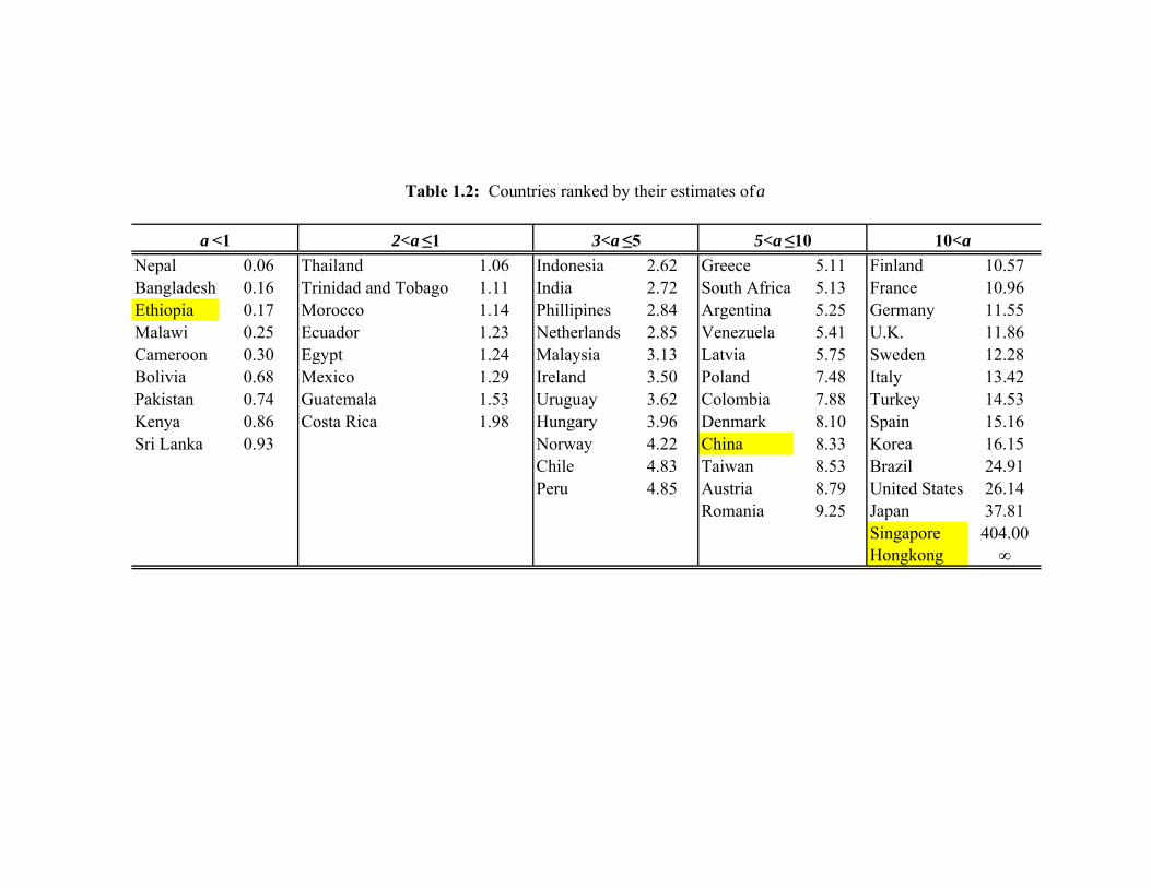
Nepal 0.06 Thailand 1.06 Indonesia 2.62 Greece 5.11 Finland 10.57Bangladesh 0.16 Trinidad and Tobago 1.11 India 2.72 South Africa 5.13 France 10.96Ethiopia 0.17 Morocco 1.14 Phillipines 2.84 Argentina 5.25 Germany 11.55Malawi 0.25 Ecuador 1.23 Netherlands 2.85 Venezuela 5.41 U.K. 11.86Cameroon 0.30 Egypt 1.24 Malaysia 3.13 Latvia 5.75 Sweden 12.28Bolivia 0.68 Mexico 1.29 Ireland 3.50 Poland 7.48 Italy 13.42Pakistan 0.74 Guatemala 1.53 Uruguay 3.62 Colombia 7.88 Turkey 14.53Kenya 0.86 Costa Rica 1.98 Hungary 3.96 Denmark 8.10 Spain 15.16Sri Lanka 0.93 Norway 4.22 China 8.33 Korea 16.15

Chile 4.83 Taiwan 8.53 Brazil 24.91Peru 4.85 Austria 8.79 United States 26.14

Romania 9.25 Japan 37.81Singapore 404.00Hongkong ∞

10<a

Table 1.2: Countries ranked by their estimates of a

a <1 2<a ≤1 3<a ≤5 5<a ≤10

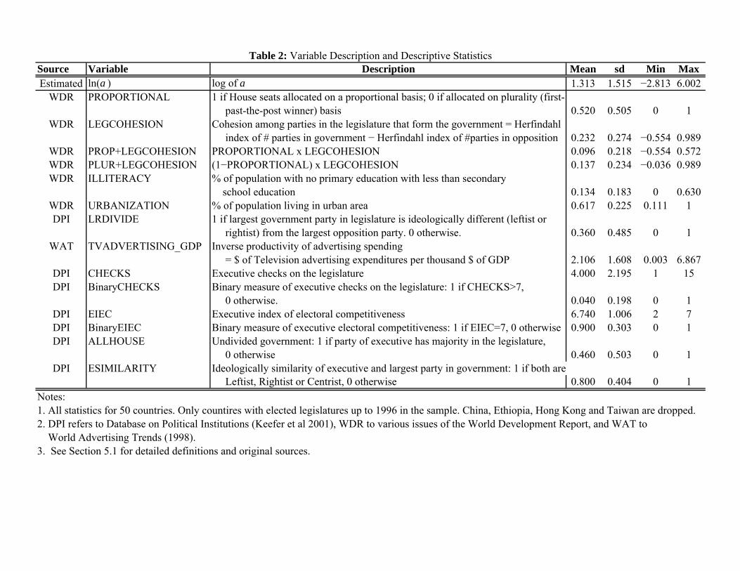
Source Variable Description Mean sd Min MaxEstimated ln(a ) log of a 1.313 1.515 −2.813 6.002

WDR PROPORTIONAL 1 if House seats allocated on a proportional basis; 0 if allocated on plurality (first- past-the-post winner) basis 0.520 0.505 0 1

WDR LEGCOHESION Cohesion among parties in the legislature that form the government = Herfindahl index of # parties in government − Herfindahl index of #parties in opposition 0.232 0.274 −0.554 0.989

WDR PROP+LEGCOHESION PROPORTIONAL x LEGCOHESION 0.096 0.218 −0.554 0.572WDR PLUR+LEGCOHESION (1−PROPORTIONAL) x LEGCOHESION 0.137 0.234 −0.036 0.989WDR ILLITERACY % of population with no primary education with less than secondary

school education 0.134 0.183 0 0.630WDR URBANIZATION % of population living in urban area 0.617 0.225 0.111 1DPI LRDIVIDE 1 if largest government party in legislature is ideologically different (leftist or

rightist) from the largest opposition party. 0 otherwise. 0.360 0.485 0 1WAT TVADVERTISING_GDP Inverse productivity of advertising spending

= $ of Television advertising expenditures per thousand $ of GDP 2.106 1.608 0.003 6.867DPI CHECKS Executive checks on the legislature 4.000 2.195 1 15DPI BinaryCHECKS Binary measure of executive checks on the legislature: 1 if CHECKS>7,

0 otherwise. 0.040 0.198 0 1DPI EIEC Executive index of electoral competitiveness 6.740 1.006 2 7DPI BinaryEIEC Binary measure of executive electoral competitiveness: 1 if EIEC=7, 0 otherwise 0.900 0.303 0 1DPI ALLHOUSE Undivided government: 1 if party of executive has majority in the legislature,

0 otherwise 0.460 0.503 0 1DPI ESIMILARITY Ideologically similarity of executive and largest party in government: 1 if both are

Leftist, Rightist or Centrist, 0 otherwise 0.800 0.404 0 1Notes:1. All statistics for 50 countries. Only countires with elected legislatures up to 1996 in the sample. China, Ethiopia, Hong Kong and Taiwan are dropped.2. DPI refers to Database on Political Institutions (Keefer et al 2001), WDR to various issues of the World Development Report, and WAT to World Advertising Trends (1998).3. See Section 5.1 for detailed definitions and original sources.

Table 2: Variable Description and Descriptive Statistics

Hypothesis Variable M1 M2EC: Proportional versus plurality (H1) PROPORTIONAL 0.037 −0.102

[0.11] [0.32]EC: Proportional versus plurality (H1.2) PROP+LEGCOHESION 1.46 0.99

[2.71]*** [1.90]*EC: Proportional versus plurality (H1.2) PLUR+LEGCOHESION 1.376 0.338

[2.55]** [0.62]EC: Uninformed voting (H2) ILLITERACY −2.759 −3.665

[2.76]*** [3.52]***EC: Uninformed voting (H2) URBANIZATION 3.821 3.175

[3.79]*** [3.89]***EC: Ideological attachment to party (H3) LRDIVIDE −0.746 −0.688

[2.20]** [2.19]**EC: Productivity of media spending (H4) TVADVERTISING_GDP 0.214 0.211

[1.65] [1.75]*LB: Executive checks on legislators (H5) CHECKS 0.153

[3.24]***LB: Executive checks on legislators (H5) BinaryCHECKS 1.809

[3.88]***LB+EC: Executive electoral competition (H6) EIEC −0.368

[3.60]***LB+EC: Executive electoral competition (H6) BinaryEIEC −1.576

[3.61]***LB: Undivided government (H7) ALLHOUSE −0.296 −0.369

[1.03] [1.31]LB: Undivided government (H7) ESIMILARITY 0.326 0.496

[0.99] [1.65]Constant 0.537 0.68

[0.59] [0.90]N 50 50Adjusted R2 0.67 0.72Tests (p -values reported): Hypothesis 1.2 0.368 0.901 Normality of ln(a) 0.209 0.209 Normality of errors 0.934 0.779

Notes: 1. Absolute t-statistics (using White-corrected standard errors) in parentheses. . * denotes statistical significance at 10%, ** at 5% and *** at 1%. 2. "EC" denotes Electoral Competition theory, "LB" denotes Legislative Bargaining theory. 3. Normality tests report p -values for the Shapiro−Wilk test.

OLS Estimates: Dependent Variable Ln(a)Table 3: Hypothesis tests about determinants of a

Theory Variable OLS1 OLS2H1 EC: Proportonal versus plurality PROPORTIONAL 0.01 −0.03H1.2 EC: Proportonal versus plurality PROP+LEGCOHESION 0.21 0.14H1.2 EC: Proportonal versus plurality PLUR+LEGCOHESION 0.21 0.05H2 EC: Uninformed voting ILLITERACY −0.33 −0.44H2 EC: Uninformed voting URBANIZATION 0.57 0.47H3 EC: Ideological attachment to party LRDIVIDE −0.24 −0.22H4 EC: Productivity of media spending TVADVERTISING_GDP 0.23 0.22H5 LB: Executive checks on legislators CHECKS 0.22H5 LB: Executive checks on legislators BinaryCHECKS 0.24H6 LB: Executive electoral competition EIEC −0.24H6 LB: Executive electoral competition BinaryEIEC −0.32H7 LB: Undivided government ALLHOUSE −0.10 −0.12H7 LB: Undivided government ESIMILARITY 0.09 0.13

Notes:1. Beta coefficients are regression coefficients of the standardized dependent variable on standardized explanatory variables.

Table 4: Beta Coefficients

M1 M2H1 PROPORTIONAL 0.052 −0.172

[0.14] [0.48]H1.2 PROP+LEGCOHESION 1.314 0.968

[1.83]* [1.41]H1.2 PLUR+LEGCOHESION 1.299 0.375

[1.63] [0.49]H2 ILLITERACY −3.299 −4.045

[2.75]*** [3.36]***H2 URBANIZATION 3.257 3.182

[3.15]*** [3.28]***H3 LRDIVIDE −0.656 −0.689

[1.81]* [1.98]*H4 TVADVERTISING_GDP 0.17 0.19

[1.38] [1.61]H5 CHECKS 0.152

[1.96]*H5 BinaryCHECKS 1.927

[2.43]**H6 EIEC −0.328

[2.17]**H6 BinaryEIEC −1.534

[3.30]***H7 ALLHOUSE −0.276 −0.28

[0.76] [0.87]H7 ESIMILARITY 0.228 0.503

[0.64] [1.45]Constant 0.788 0.706

[0.59] [0.77]N 50 50Adjusted R2 0.69 0.75Note:1. Absolute t -statistics in parentheses: * denotes staticial significance at 10%; ** at 5%, and *** at 1%.2. Weighted regressions, with weights inversely related to residuals.

Table 5: Robust (to Outliers) regressionsDependent variable: ln(a )

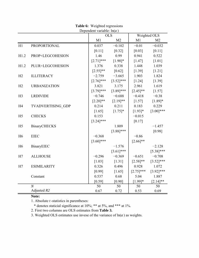
M1 M2 M1 M2H1 PROPORTIONAL 0.037 −0.102 −0.01 −0.032

[0.11] [0.32] [0.03] [0.11]H1.2 PROP+LEGCOHESION 1.46 0.99 0.941 0.522

[2.71]*** [1.90]* [1.47] [1.01]H1.2 PLUR+LEGCOHESION 1.376 0.338 1.448 1.039

[2.55]** [0.62] [1.39] [1.21]H2 ILLITERACY −2.759 −3.665 1.903 1.824

[2.76]*** [3.52]*** [1.24] [1.39]H2 URBANIZATION 3.821 3.175 2.961 1.619

[3.79]*** [3.89]*** [2.45]** [1.57]H3 LRDIVIDE −0.746 −0.688 −0.418 −0.38

[2.20]** [2.19]** [1.57] [1.89]*H4 TVADVERTISING_GDP 0.214 0.211 0.183 0.229

[1.65] [1.75]* [1.93]* [3.00]***H5 CHECKS 0.153 −0.015

[3.24]*** [0.17]H5 BinaryCHECKS 1.809 −1.457

[3.88]*** [0.98]H6 EIEC −0.368 −0.86

[3.60]*** [2.66]**H6 BinaryEIEC −1.576 −2.128

[3.61]*** [5.38]***H7 ALLHOUSE −0.296 −0.369 −0.651 −0.708

[1.03] [1.31] [2.58]** [3.52]***H7 ESIMILARITY 0.326 0.496 0.928 1.072

[0.99] [1.65] [2.75]*** [3.92]***Constant 0.537 0.68 5.04 1.887

[0.59] [0.90] [1.99]* [2.14]**N 50 50 50 50Adjusted R2 0.67 0.72 0.53 0.69Note:1. Absolute t -statistics in parentheses: * denotes staticial significance at 10%; ** at 5%, and *** at 1%.2. First two columns are OLS estimates from Table 3.3. Weighted OLS estimates use invese of the variance of ln(a ) as weights.

OLS Weighted OLS

Table 6: Weighted regressionsDependent variable: ln(a )

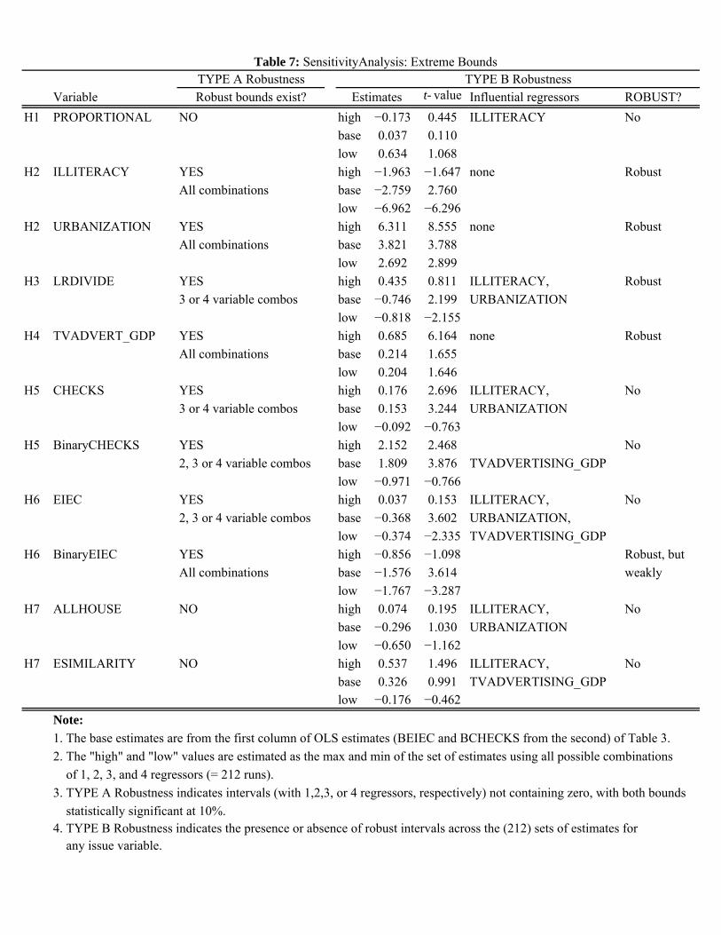
TYPE A RobustnessVariable Robust bounds exist? t- value Influential regressors ROBUST?

H1 PROPORTIONAL NO high −0.173 0.445 ILLITERACY Nobase 0.037 0.110low 0.634 1.068

H2 ILLITERACY YES high −1.963 −1.647 none Robust All combinations base −2.759 2.760

low −6.962 −6.296H2 URBANIZATION YES high 6.311 8.555 none Robust

All combinations base 3.821 3.788low 2.692 2.899

H3 LRDIVIDE YES high 0.435 0.811 ILLITERACY, Robust 3 or 4 variable combos base −0.746 2.199 URBANIZATION

low −0.818 −2.155H4 TVADVERT_GDP YES high 0.685 6.164 none Robust

All combinations base 0.214 1.655low 0.204 1.646

H5 CHECKS YES high 0.176 2.696 ILLITERACY, No3 or 4 variable combos base 0.153 3.244 URBANIZATION

low −0.092 −0.763H5 BinaryCHECKS YES high 2.152 2.468 No

2, 3 or 4 variable combos base 1.809 3.876 TVADVERTISING_GDPlow −0.971 −0.766

H6 EIEC YES high 0.037 0.153 ILLITERACY, No2, 3 or 4 variable combos base −0.368 3.602 URBANIZATION,

low −0.374 −2.335 TVADVERTISING_GDPH6 BinaryEIEC YES high −0.856 −1.098 Robust, but

All combinations base −1.576 3.614 weakly low −1.767 −3.287

H7 ALLHOUSE NO high 0.074 0.195 ILLITERACY, Nobase −0.296 1.030 URBANIZATIONlow −0.650 −1.162

H7 ESIMILARITY NO high 0.537 1.496 ILLITERACY, Nobase 0.326 0.991 TVADVERTISING_GDPlow −0.176 −0.462

Note: 1. The base estimates are from the first column of OLS estimates (BEIEC and BCHECKS from the second) of Table 3.2. The "high" and "low" values are estimated as the max and min of the set of estimates using all possible combinations of 1, 2, 3, and 4 regressors (= 212 runs).3. TYPE A Robustness indicates intervals (with 1,2,3, or 4 regressors, respectively) not containing zero, with both bounds statistically significant at 10%.4. TYPE B Robustness indicates the presence or absence of robust intervals across the (212) sets of estimates for any issue variable.

Table 7: SensitivityAnalysis: Extreme Bounds

EstimatesTYPE B Robustness