what is a np problem? given an instance of the problem, v, and a ‘certificate’, c, we can verify...
TRANSCRIPT


What is a NP problem?What is a NP problem?
Given an instance of the problem, Given an instance of the problem, VV, , and a ‘certificate’, and a ‘certificate’, CC, we can verify , we can verify VV is in the language in polynomial timeis in the language in polynomial time
All problems in P are NP problemsAll problems in P are NP problems Why?Why?
What is NP-Complete?What is NP-Complete?
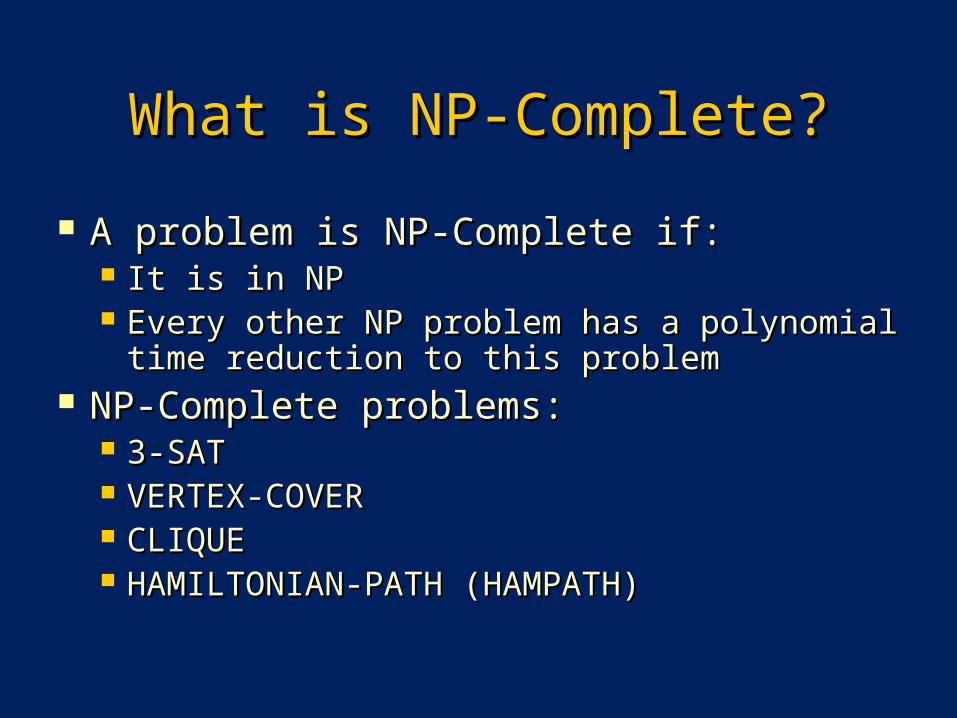
A problem is NP-Complete if:A problem is NP-Complete if: It is in NPIt is in NP Every other NP problem has a polynomial Every other NP problem has a polynomial
time reduction to this problemtime reduction to this problem NP-Complete problems:NP-Complete problems:
3-SAT3-SAT VERTEX-COVERVERTEX-COVER CLIQUECLIQUE HAMILTONIAN-PATH (HAMPATH)HAMILTONIAN-PATH (HAMPATH)

DilemmaDilemma
NP problems need solutions in real-NP problems need solutions in real-lifelife
We only know exponential algorithmsWe only know exponential algorithms What do we do?What do we do?

55
A SolutionA Solution There are many important NP-There are many important NP-
Complete problemsComplete problems There is no fast solution !There is no fast solution !
But we want the answer …But we want the answer … If the input is small use backtrack.If the input is small use backtrack. Isolate the problem into P-problems !Isolate the problem into P-problems ! Find the Find the Near-OptimalNear-Optimal solution in solution in
polynomial time.polynomial time.
AccuracyAccuracy
NP problems are often optimization NP problems are often optimization problemsproblems
It’s hard to find the EXACT answerIt’s hard to find the EXACT answer Maybe we just want to know our Maybe we just want to know our
answer is close to the exact answer?answer is close to the exact answer?

Approximation AlgorithmsApproximation Algorithms
Can be created for optimization Can be created for optimization problemsproblems
The exact answer for an instance is OPTThe exact answer for an instance is OPT The approximate answer will never be The approximate answer will never be
far from OPTfar from OPT
We CANNOT approximate decision We CANNOT approximate decision problemsproblems

88
Performance ratiosPerformance ratios We are going to find a Near-We are going to find a Near-
Optimal solution for a given Optimal solution for a given problem.problem.
We assume two hypothesis :We assume two hypothesis : Each potential solution has a positive Each potential solution has a positive
cost.cost. The problem may be either a The problem may be either a
maximization or a minimization maximization or a minimization problem on the cost.problem on the cost.

99
Performance ratios …Performance ratios … If for any input of size n, the cost C If for any input of size n, the cost C
of the solution produced by the of the solution produced by the algorithm is within a factor of algorithm is within a factor of ρ(n)ρ(n) of the cost C* of an optimal of the cost C* of an optimal solution:solution:
Max ( C/C* , C*/C ) ≤ ρ(n)Max ( C/C* , C*/C ) ≤ ρ(n) We call this algorithm as an ρ(n)-We call this algorithm as an ρ(n)-
approximation algorithm.approximation algorithm.

Performance ratios …Performance ratios … In Maximization problems:In Maximization problems:
C*/ρ(n) ≤ C ≤ C* C*/ρ(n) ≤ C ≤ C* In Minimization Problems:In Minimization Problems:
C* ≤ C ≤ ρ(n)C*C* ≤ C ≤ ρ(n)C* ρ(n) is never less than 1. ρ(n) is never less than 1. A 1-approximation algorithm is the optimal A 1-approximation algorithm is the optimal
solution.solution. The goal is to find a polynomial-time The goal is to find a polynomial-time
approximation algorithm with small approximation algorithm with small constant approximation ratios.constant approximation ratios.

1111
Approximation schemeApproximation scheme Approximation schemeApproximation scheme is an is an
approximation algorithm that takes Є>0 approximation algorithm that takes Є>0 as an input such that for any fixed Є>0 as an input such that for any fixed Є>0 the scheme is (1+Є)-approximation the scheme is (1+Є)-approximation algorithm.algorithm.
Polynomial-time approximation Polynomial-time approximation scheme scheme is such algorithm that runs in is such algorithm that runs in time polynomial in the size of input.time polynomial in the size of input. As the Є decreases the running time of the As the Є decreases the running time of the
algorithm can increase rapidly:algorithm can increase rapidly: For example it might be O(nFor example it might be O(n2/Є2/Є))
1212
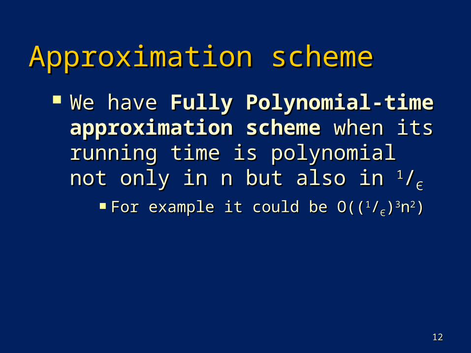
Approximation schemeApproximation scheme We haveWe have Fully Polynomial-time Fully Polynomial-time
approximation scheme approximation scheme when its when its running time is polynomial not only running time is polynomial not only in n but also in in n but also in 11//ЄЄ
For example it could be O((For example it could be O((11//ЄЄ))33nn22))

1313
Some examples:Some examples:
Vertex cover problem.Vertex cover problem. Traveling salesman problem.Traveling salesman problem. Set cover problem.Set cover problem.

VERTEX-COVERVERTEX-COVER
Given a graph, G, return the smallest Given a graph, G, return the smallest set of vertices such that all edges set of vertices such that all edges have an end point in the sethave an end point in the set

1515
The vertex-cover problemThe vertex-cover problem A vertex-cover of an undirected A vertex-cover of an undirected
graph G is a subset of its vertices graph G is a subset of its vertices such that it includes at least one such that it includes at least one end of each edge.end of each edge.
The problem is to find minimum size The problem is to find minimum size of vertex-cover of the given graph.of vertex-cover of the given graph.
This problem is an NP-Complete This problem is an NP-Complete problem.problem.

1616
The vertex-cover problemThe vertex-cover problem ……
Finding the optimal solution is hard Finding the optimal solution is hard (it’s NP!) but finding a near-optimal (it’s NP!) but finding a near-optimal solution is easy.solution is easy.
There is an 2-approximation There is an 2-approximation algorithm:algorithm: It returns a vertex-cover not more It returns a vertex-cover not more
than twice of the size optimal than twice of the size optimal solution.solution.

1717
The vertex-cover problemThe vertex-cover problem ……
APPROX-VERTEX-COVER(G)APPROX-VERTEX-COVER(G)
1 1 C ← ØC ← Ø2 2 E′ ← E[G]E′ ← E[G]3 3 while while E′ ≠ ØE′ ≠ Ø4 4 do do let (u, v) be an arbitrary edge of E′let (u, v) be an arbitrary edge of E′5 5 C ← C U {u, v}C ← C U {u, v}6 6 remove every edge in E′ incident on u or remove every edge in E′ incident on u or
vv7 7 return return CC

1818
The vertex-cover problemThe vertex-cover problem ……
OptimalSize=3
Near Optimalsize=6

1919
The vertex-cover problemThe vertex-cover problem ……
This is a polynomial-time This is a polynomial-time
2-aproximation algorithm. (Why?)2-aproximation algorithm. (Why?) Because:Because:
APPROX-VERTEX-COVER is O(V+E)APPROX-VERTEX-COVER is O(V+E) |C*| ≥ |A||C*| ≥ |A|
|C| = 2|A||C| = 2|A|
|C| ≤ 2|C*||C| ≤ 2|C*|Optimal
Selected Edges
Selected Vertices
Minimum Spanning TreeMinimum Spanning Tree
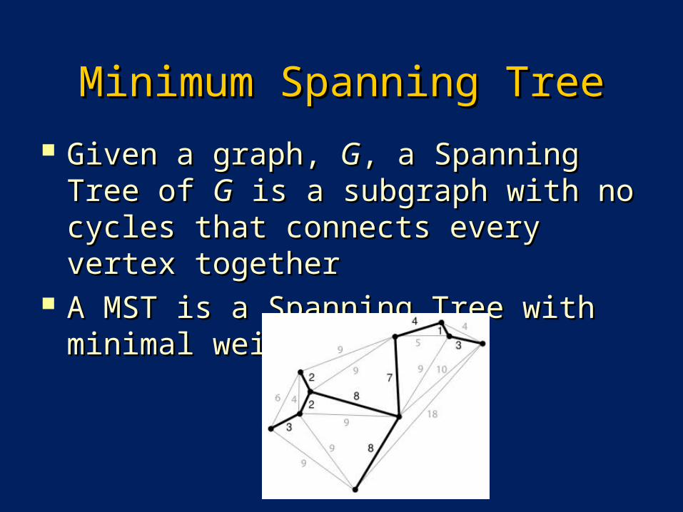
Given a graph, Given a graph, GG, a Spanning Tree of , a Spanning Tree of GG is a subgraph with no cycles that is a subgraph with no cycles that connects every vertex togetherconnects every vertex together
A MST is a Spanning Tree with A MST is a Spanning Tree with minimal weightminimal weight
Finding a MSTFinding a MST
Finding a MST can be done in Finding a MST can be done in polynomial time using PRIM’S polynomial time using PRIM’S ALGORITHM or KRUSKAL’S ALGORITHM or KRUSKAL’S ALGORITHMALGORITHM
Both are greedy algorithmsBoth are greedy algorithms

HAMILTONIAN CYCLEHAMILTONIAN CYCLE
Given a graph, G, find a cycle that Given a graph, G, find a cycle that visits every vertex exactly oncevisits every vertex exactly once
TSP version: Find the path with the TSP version: Find the path with the minimum weightminimum weight

MST vs HAM-CYCLEMST vs HAM-CYCLE
Any HAM-CYCLE becomes a Spanning Any HAM-CYCLE becomes a Spanning Tree by removing an edgeTree by removing an edge
cost(MST) ≤ cost(min-HAM-CYCLE)cost(MST) ≤ cost(min-HAM-CYCLE)
2424
Traveling salesman problemTraveling salesman problem Given an undirected complete Given an undirected complete
weighted graph G we are to find a weighted graph G we are to find a minimum cost Hamiltonian cycle.minimum cost Hamiltonian cycle.
Satisfying triangle inequality or not Satisfying triangle inequality or not this problem is NP-Complete. this problem is NP-Complete.
The problem is called The problem is called Euclidean Euclidean TSPTSP..

2525
Traveling salesman problemTraveling salesman problem Near Optimal solutionNear Optimal solution
FasterFaster Easier to implement.Easier to implement.
2626
Euclidian Traveling Salesman Euclidian Traveling Salesman ProblemProblem
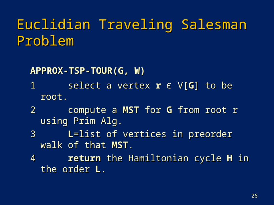
APPROX-TSP-TOUR(G, W)APPROX-TSP-TOUR(G, W)
1 1 select a vertex select a vertex rr ЄЄ V[V[GG] to be root.] to be root.
2 2 compute a compute a MSTMST for for GG from root r using Prim from root r using Prim Alg.Alg.
3 3 LL=list of vertices in preorder walk of that =list of vertices in preorder walk of that MSTMST..
4 4 returnreturn the Hamiltonian cycle the Hamiltonian cycle HH in the order in the order LL..

2727
Euclidian Traveling Salesman Euclidian Traveling Salesman ProblemProblem
root
MST
Pre-Order walk
Hamiltonian Cycle

2828
Traveling salesman problemTraveling salesman problem This is polynomial-time 2-This is polynomial-time 2-
approximation algorithm. (Why?)approximation algorithm. (Why?) Because:Because:
APPROX-TSP-TOUR is O(VAPPROX-TSP-TOUR is O(V22)) C(MST)C(MST) ≤ C(H*) H*: optimal soln≤ C(H*) H*: optimal soln
C(W)=2C(MST) W: Preorder walkC(W)=2C(MST) W: Preorder walk
C(W)≤2C(H*)C(W)≤2C(H*)
C(H)≤C(W) H: approx soln &C(H)≤C(W) H: approx soln &
C(H)≤2C(H*) triangle C(H)≤2C(H*) triangle inequalityinequality
Optimal
Pre-order
Solution

EULER CYCLEEULER CYCLE Given a graph, G, find a cycle that Given a graph, G, find a cycle that
visits every edge exactly oncevisits every edge exactly once Necessary & Sufficient Conditions: Necessary & Sufficient Conditions:
G is connected and every vertex is G is connected and every vertex is even degree.even degree.
Algorithm (O(nAlgorithm (O(n22)): )):
1.1. Repeatedly use DFS to find and Repeatedly use DFS to find and remove a cycle from Gremove a cycle from G
2.2. Merge all the cycles into one Merge all the cycles into one cycle.cycle.
Min-Weight MatchingMin-Weight Matching
Algorithm (O(nAlgorithm (O(n33)): Formulated as a )): Formulated as a linear programming problem, but linear programming problem, but solved using a special algorithm.solved using a special algorithm.
Given a complete weighted graph of Given a complete weighted graph of even nodes, G, find a perfect even nodes, G, find a perfect matching of minimum total weightmatching of minimum total weight
3131
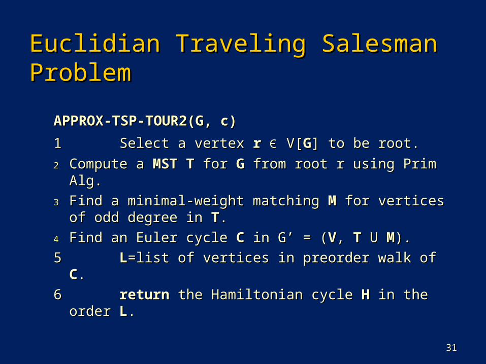
Euclidian Traveling Salesman Euclidian Traveling Salesman ProblemProblem
APPROX-TSP-TOUR2(G, c)APPROX-TSP-TOUR2(G, c)
1 1 Select a vertex Select a vertex rr ЄЄ V[V[GG] to be root.] to be root.
22 Compute a Compute a MSTMST TT for for GG from root r using Prim from root r using Prim Alg.Alg.
33 Find a minimal-weight matching Find a minimal-weight matching MM for vertices for vertices of odd degree in of odd degree in TT..
44 Find an Euler cycle Find an Euler cycle CC in G’ = ( in G’ = (VV, , TT U U MM).).
5 5 LL=list of vertices in preorder walk of =list of vertices in preorder walk of CC..
6 6 returnreturn the Hamiltonian cycle the Hamiltonian cycle HH in the order in the order LL..

3232
Euclidian Traveling Salesman Euclidian Traveling Salesman ProblemProblem
MST Min Matching
Euler Cycle HAM-Cycle

3333
Time ComplexityTime Complexity
APPROX-TSP-TOUR2(G, c)APPROX-TSP-TOUR2(G, c)
1 1 Select a vertex Select a vertex rr ЄЄ V[V[GG] to be root.] to be root.
22 Compute a Compute a MSTMST TT for for GG from root r from root r using Prim Alg.using Prim Alg.
33 Find a minimal-weight matching Find a minimal-weight matching MM for for vertices of odd degree in vertices of odd degree in TT..
44 Find an Euler cycle Find an Euler cycle AA in G’ = ( in G’ = (VV, , TT U U MM).).
5 5 LL=list of vertices in preorder walk of =list of vertices in preorder walk of AA..
6 6 returnreturn the Hamiltonian cycle the Hamiltonian cycle HH in order in order LL..
O(1)O(n lg n)
O(n3)
O(n2)
O(n)
3434
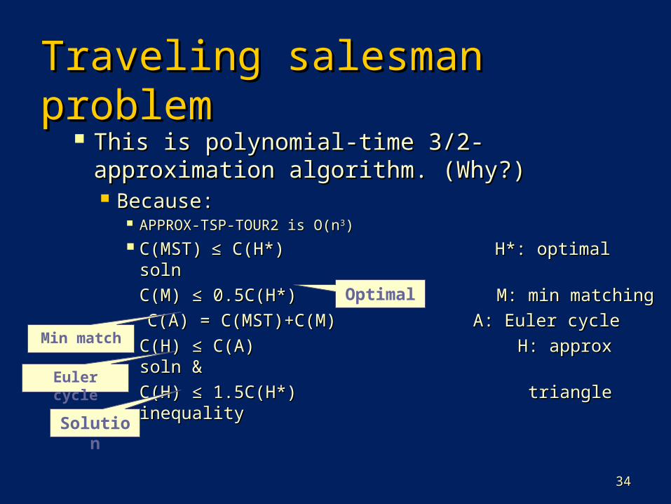
Traveling salesman problemTraveling salesman problem This is polynomial-time 3/2-This is polynomial-time 3/2-
approximation algorithm. (Why?)approximation algorithm. (Why?) Because:Because:
APPROX-TSP-TOUR2 is O(nAPPROX-TSP-TOUR2 is O(n33)) C(MST)C(MST) ≤ C(H*) H*: optimal soln≤ C(H*) H*: optimal soln
C(M) ≤ 0.5C(H*) M: min matchingC(M) ≤ 0.5C(H*) M: min matching
C(A) = C(MST)+C(M) A: Euler cycleC(A) = C(MST)+C(M) A: Euler cycle
C(H) ≤ C(A) H: approx soln &C(H) ≤ C(A) H: approx soln &
C(H) ≤ 1.5C(H*) triangle C(H) ≤ 1.5C(H*) triangle inequalityinequality
Optimal
Euler cycle
Solution
Min match
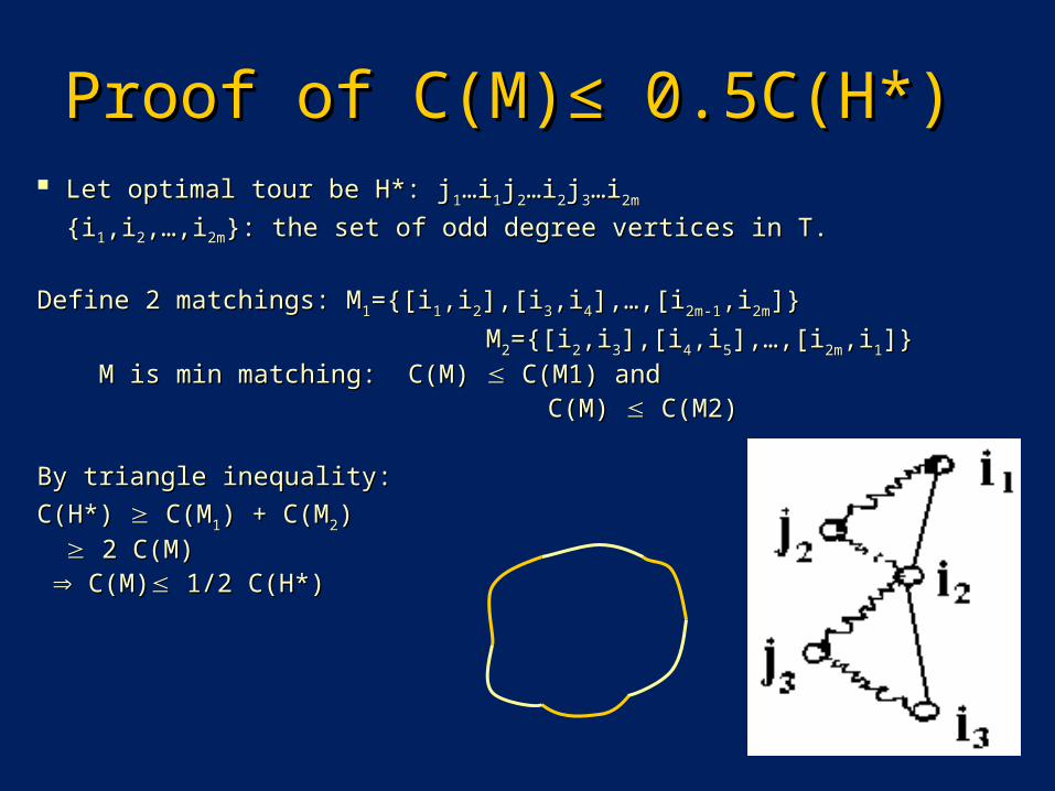
Proof of C(M)≤ 0.5C(H*) Proof of C(M)≤ 0.5C(H*) Let optimal tour be H*: jLet optimal tour be H*: j11……ii11jj22……ii22jj33……ii2m2m
{i{i11,i,i22,,……,i,i2m2m}: the set of odd degree vertices in T.}: the set of odd degree vertices in T.
Define 2 matchings: MDefine 2 matchings: M11={[i={[i11,i,i22],[i],[i33,i,i44],],……,[i,[i2m-12m-1,i,i2m2m]}]}
MM22={[i={[i22,i,i33],[i],[i44,i,i55],],……,[i,[i2m2m,i,i11]} ]} M is min matching: C(M) M is min matching: C(M) C(M1) and C(M1) and C(M) C(M) C(M2) C(M2)
By triangle inequality:By triangle inequality:
C(H*) C(H*) C(M C(M11) + C(M) + C(M22) ) 2 C(M) 2 C(M)
CC(M)(M) 1/2 C(H*) 1/2 C(H*)

3636
TSP In GeneralTSP In General
Theorem: Theorem: If P ≠ NP, then for any constant ρ>1, If P ≠ NP, then for any constant ρ>1, there is no polynomial time ρ-approximation there is no polynomial time ρ-approximation algorithm. algorithm.
Proof: If we have a polynomial time ρ-approximation Proof: If we have a polynomial time ρ-approximation algorithm for TSP, we can find a tour of cost ρH*. algorithm for TSP, we can find a tour of cost ρH*.
c(u,w) = if ((u,w) in E) then 1 else ρ|V|+1c(u,w) = if ((u,w) in E) then 1 else ρ|V|+1 The optimal cost H* of a TSP tour is |V|.The optimal cost H* of a TSP tour is |V|. G has a Ham-cycle iff TSP has a tour of cost G has a Ham-cycle iff TSP has a tour of cost ρ|V|.ρ|V|. If a TSP tour has one edge of cost ρ|V|+1, then the If a TSP tour has one edge of cost ρ|V|+1, then the
total cost is (total cost is (ρ|V|+1)ρ|V|+1)++|V|-1|V|-1>ρ|V|>ρ|V|
Selected edge not in E
Rest of edges

3737
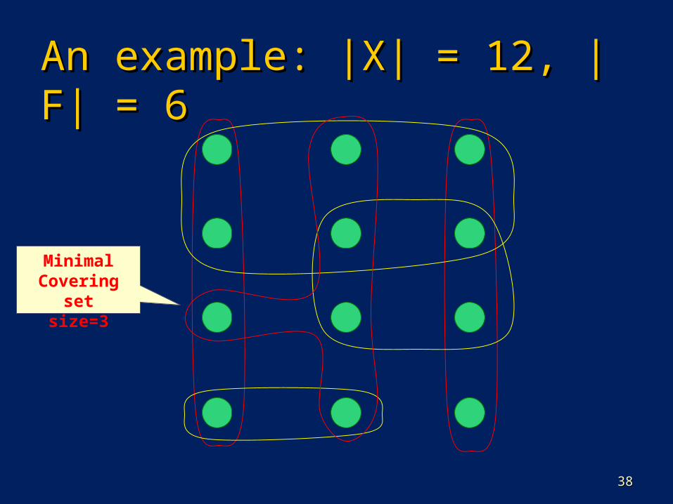
The Set-Cover ProblemThe Set-Cover Problem Instance (X, F) :Instance (X, F) :
X : a finite set of elements.X : a finite set of elements. F : family of subsets of X.F : family of subsets of X. Solution C : subset of F that includes all Solution C : subset of F that includes all
the members of X.the members of X. Set-Cover is in NPSet-Cover is in NP Set-Cover is NP-hard, as it’s a Set-Cover is NP-hard, as it’s a
generalization of vertex-cover generalization of vertex-cover problem.problem.
3838
An example: |X| = 12, |F| = An example: |X| = 12, |F| = 66
Minimal Covering
setsize=3

3939
A Greedy AlgorithmA Greedy AlgorithmGREEDY-SET-COVER(X,F)GREEDY-SET-COVER(X,F)
1 M ← X1 M ← X
2 C ← Ø2 C ← Ø
3 3 while while M ≠ Ø M ≠ Ø dodo
44 select S select S ЄЄ F that maximizes |S F that maximizes |S חח M|M|
55 M ← M – SM ← M – S
66 C ← C U {S}C ← C U {S}
7 7 return return CC

4040
Not optimal …Not optimal …
3rd chose
1st chose
2nd chose
4th chose
GreedyCovering
setsize=4

4141
This greedy algorithm is This greedy algorithm is polynomial-time ρ(n)-polynomial-time ρ(n)-approximation algorithmapproximation algorithm
ρ(n)=lg(n)ρ(n)=lg(n)
Set-Cover …Set-Cover …

The bin packing problem The bin packing problem n items an items a11, a, a22, , ……, a, ann, 0, 0 a aii 1, 1 1, 1 i i n, to n, to
determine the minimum number of bins of determine the minimum number of bins of unit capacity to accommodate all n items. unit capacity to accommodate all n items.
E.g. n = 5, {0.3, 0.5, 0.8, 0.2 0.4} E.g. n = 5, {0.3, 0.5, 0.8, 0.2 0.4}
The bin packing problem is NP-hard.
APPROXIMATE BIN PACKINGAPPROXIMATE BIN PACKING
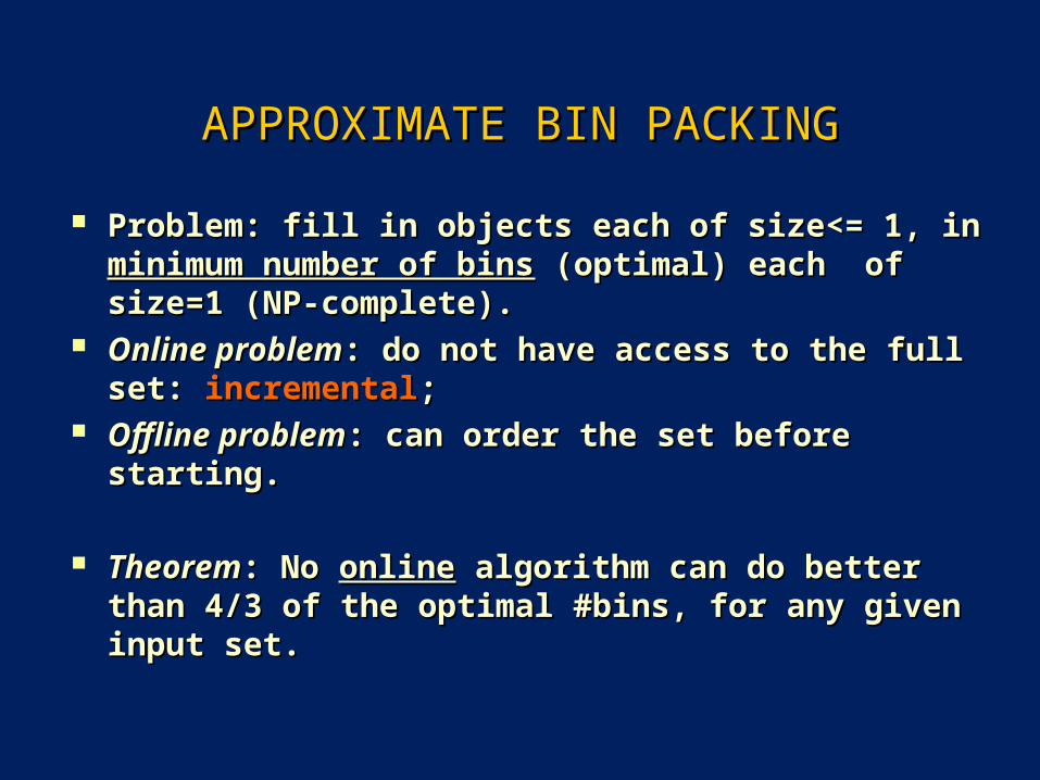
Problem: fill in objects each of size<= 1, in Problem: fill in objects each of size<= 1, in minimum number of binsminimum number of bins (optimal) each of (optimal) each of size=1 (NP-complete).size=1 (NP-complete).
Online problemOnline problem: do not have access to the full : do not have access to the full set: set: incrementalincremental; ;
Offline problemOffline problem: can order the set before : can order the set before starting.starting.
TheoremTheorem: No : No onlineonline algorithm can do better algorithm can do better than 4/3 of the optimal #bins, for any given than 4/3 of the optimal #bins, for any given input set.input set.
NEXT-FIT ONLINE BIN-PACKINGNEXT-FIT ONLINE BIN-PACKING
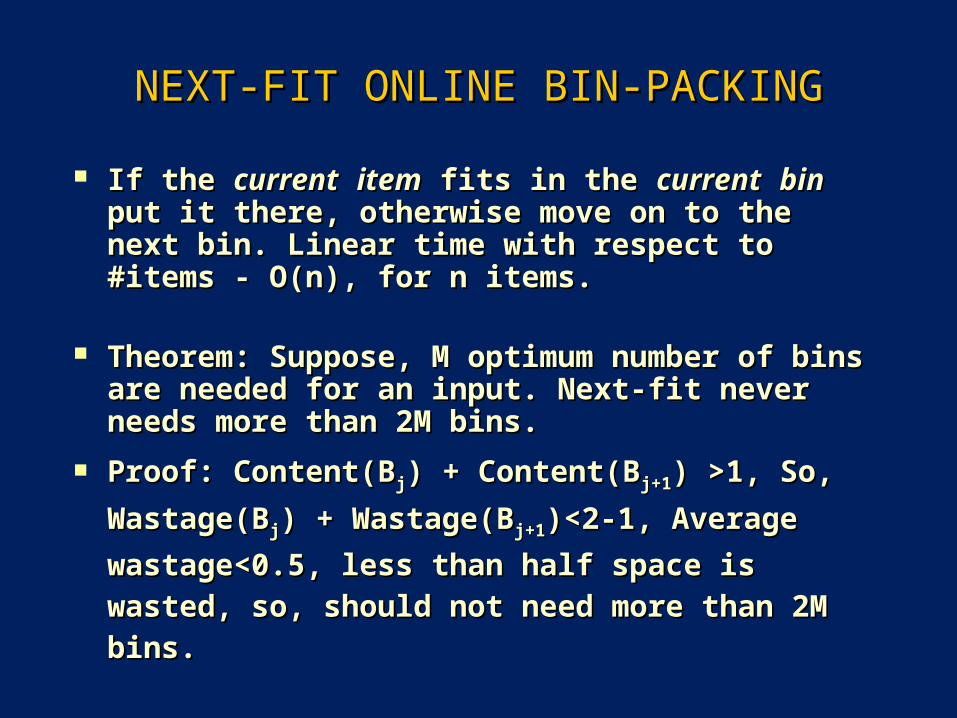
If the If the currentcurrent itemitem fits in the fits in the currentcurrent binbin put it there, otherwise move on to the put it there, otherwise move on to the next bin. Linear time with respect to next bin. Linear time with respect to #items - O(n), for n items.#items - O(n), for n items.
Theorem: Suppose, M optimum number of Theorem: Suppose, M optimum number of bins are needed for an input. Next-fit bins are needed for an input. Next-fit never needs more than 2M bins. never needs more than 2M bins.
Proof: Content(BProof: Content(Bjj) + Content(B) + Content(Bj+1j+1) >1, So, ) >1, So,
Wastage(BWastage(Bjj) + Wastage(B) + Wastage(Bj+1j+1)<2-1, Average )<2-1, Average
wastage<0.5, less than half space is wastage<0.5, less than half space is wasted, so, should not need more than 2M wasted, so, should not need more than 2M bins. bins.

FIRST-FIT ONLINE BIN-PACKINGFIRST-FIT ONLINE BIN-PACKING Scan the existing bins, starting from the first bin, to Scan the existing bins, starting from the first bin, to
find the place for the next item, if none exists create find the place for the next item, if none exists create a new bin. O(Na new bin. O(N22) naïve, O(N logN) possible, for N ) naïve, O(N logN) possible, for N items.items.
Obviously cannot need more than 2M bins! Wastes Obviously cannot need more than 2M bins! Wastes less than Next-fit.less than Next-fit.
Theorem: Never needs more than Ceiling(1.7M). Theorem: Never needs more than Ceiling(1.7M).
Proof: too complicated.Proof: too complicated.
For random (Gaussian) input sequence, it takes 2% For random (Gaussian) input sequence, it takes 2% more than optimal, observed empirically. Great!more than optimal, observed empirically. Great!

BEST-FIT ONLINE BIN-PACKINGBEST-FIT ONLINE BIN-PACKING
Scan to find the tightest spot for each item Scan to find the tightest spot for each item (reduce wastage even further than the (reduce wastage even further than the previous algorithms), if none exists create a previous algorithms), if none exists create a new bin.new bin.
Does not improve over First-Fit in worst Does not improve over First-Fit in worst case in optimality, but does not take more case in optimality, but does not take more worst-case time either! Easy to code.worst-case time either! Easy to code.
OFFLINE BIN-PACKINGOFFLINE BIN-PACKING
Create a non-increasing order (larger to smaller) Create a non-increasing order (larger to smaller) of items first and then apply some of the same of items first and then apply some of the same algorithms as before.algorithms as before.
TheoremTheorem: : If M is optimum #bins, then First-fit-If M is optimum #bins, then First-fit-offline will not take more than M + (1/3)M #bins.offline will not take more than M + (1/3)M #bins.

Polynomial-Time Polynomial-Time Approximation SchemesApproximation Schemes
A problem L has a A problem L has a fully polynomial-time fully polynomial-time approximation approximation
scheme (FPTAS)scheme (FPTAS) if it has a polynomial-time (in n if it has a polynomial-time (in n and 1/ε)and 1/ε)
(1+ε)-approximation algorithm, for any fixed ε >0.(1+ε)-approximation algorithm, for any fixed ε >0.
0/1 Knapsack has a FPTAS, with a running time 0/1 Knapsack has a FPTAS, with a running time that is O(nthat is O(n33 / ε). / ε).

49
Knapsack Problem
Knapsack problem. Given n objects and a "knapsack." Item i has value vi > 0 and weighs wi > 0. Knapsack can carry weight up to W. Goal: fill knapsack so as to maximize total value.
Ex: { 3, 4 } has value 40.1
Value
18
22
28
1
Weight
5
6
6 2
7
Item
1
3
4
5
2W = 11
we'll assume wi W

50
Knapsack is NP-Complete
KNAPSACK: Given a finite set X, nonnegative weights wi,
nonnegative values vi, a weight limit W, and a target value V, is
there a subset S X such that:
SUBSET-SUM: Given a finite set X, nonnegative values ui, and an
integer U, is there a subset S X whose elements sum to exactly U?
Claim. SUBSET-SUM P KNAPSACK.Pf. Given instance (u1, …, un, U) of SUBSET-SUM, create KNAPSACK
instance:
wiiS
W
viiS
V
vi wi ui uiiS U
V W U uiiS U

51
Knapsack Problem: Dynamic Programming 1
Def. OPT(i, w) = max value subset of items 1,..., i with weight limit w.
Case 1: OPT does not select item i.– OPT selects best of 1, …, i–1 using up to weight limit w
Case 2: OPT selects item i.– new weight limit = w – wi
– OPT selects best of 1, …, i–1 using up to weight limit w – wi
Running time. O(n W). W = weight limit. Not polynomial in input size!

52
Knapsack Problem: Dynamic Programming II
Def. OPT(i, v) = min weight subset of items 1, …, i that yields value exactly v.
Case 1: OPT does not select item i.– OPT selects best of 1, …, i-1 that achieves exactly value v
Case 2: OPT selects item i.– consumes weight wi, new value needed = v – vi
– OPT selects best of 1, …, i-1 that achieves exactly value v

53
Knapsack: FPTAS
1
Value
3
4
6
1
Weight
5
6
1 2
7
Item
1
3
4
5
2
W = 11
0 1 2 3 4 5 6 7 8 9 10
11
12
13
14
15
0 0 x x x x x x x x x x x x x x x
1 0
2 0
3 0
4 0
5 0
i = 0 or v = 0

54
Knapsack: FPTAS
1
Value
3
4
6
1
Weight
5
6
1 2
7
Item
1
3
4
5
2
W = 11
0 1 2 3 4 5 6 7 8 9 10
11
12
13
14
15
0 0 x x x x x x x x x x x x x x x
1 0 1 x x x x x x x x x x x x x x
2 0
3 0
4 0
5 0
i = 1 , v = …

55
Knapsack: FPTAS
1
Value
3
4
6
1
Weight
5
6
1 2
7
Item
1
3
4
5
2
W = 11
0 1 2 3 4 5 6 7 8 9 10
11
12
13
14
15
0 0 x x x x x x x x x x x x x x x
1 0 1 x x x x x x x x x x x x x x
2 0 1 3 x x x x x x x x x x x x x
3 0
4 0
5 0
i = 2 , v = …

56
Knapsack: FPTAS
1
Value
3
4
6
1
Weight
5
6
1 2
7
Item
1
3
4
5
2
W = 11
0 1 2 3 4 5 6 7 8 9 10
11
12
13
14
15
0 0 x x x x x x x x x x x x x x x
1 0 1 x x x x x x x x x x x x x x
2 0 1 3 x x x x x x x x x x x x x
3 0 1 3 5 6 8 x x x x x x x x x x
4 0
5 0
i = 3 , v = …

57
Knapsack: FPTAS
1
Value
3
4
6
1
Weight
5
6
1 2
7
Item
1
3
4
5
2
W = 11
0 1 2 3 4 5 6 7 8 9 10
11
12
13
14
15
0 0 x x x x x x x x x x x x x x x
1 0 1 x x x x x x x x x x x x x x
2 0 1 3 x x x x x x x x x x x x x
3 0 1 3 5 6 8 x x x x x x x x x x
4 0 1 3 5 6 7 9 11
12
14
x x x x x x
5 0
i = 4, v = …
58
Knapsack: FPTAS
1
Value
3
4
6
1
Weight
5
6
1 2
7
Item
1
3
4
5
2
W = 11
0 1 2 3 4 5 6 7 8 9 10
11
12
13
14
15
0 0 x x x x x x x x x x x x x x x
1 0 1 x x x x x x x x x x x x x x
2 0 1 3 x x x x x x x x x x x x x
3 0 1 3 5 6 8 x x x x x x x x x x
4 0 1 3 5 6 7 9 11
12
14
x x x x x x
5 0 1 3 5 6 7 7 8 10
12
13
14
16
18
19
21
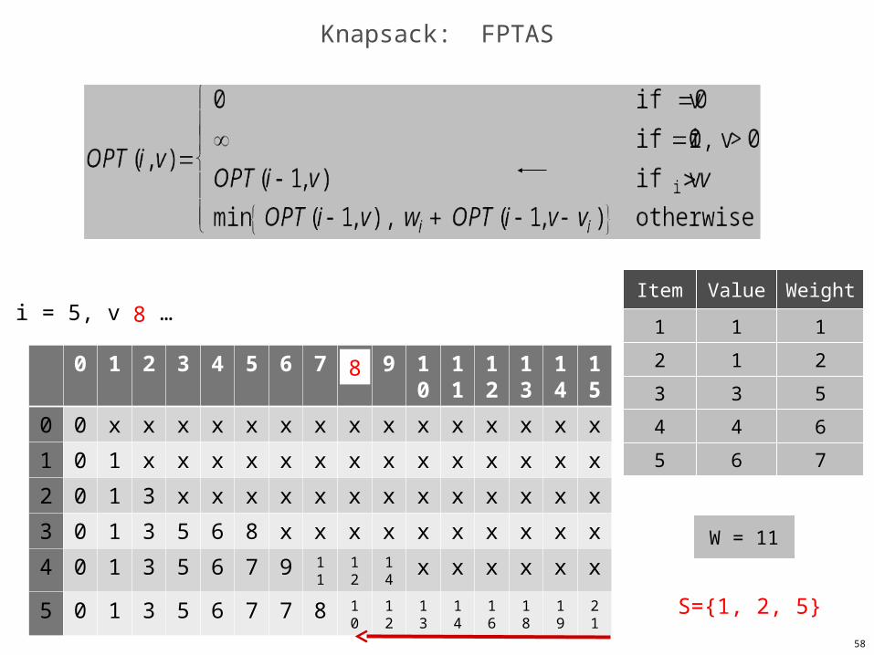
i = 5, v = …
8
8
S={1, 2, 5}

59
Knapsack: FPTAS Tracing Solution
1
Value
3
4
6
1
Weight
5
6
1 2
7
Item
1
3
4
5
2
W = 11
0 1 2 3 4 5 6 7 8 9 10
11
12
13
14
15
0 0 x x x x x x x x x x x x x x x
1 0 1 x x x x x x x x x x x x x x
2 0 1 3 x x x x x x x x x x x x x
3 0 1 3 5 6 8 x x x x x x x x x x
4 0 1 3 5 6 7 9 11
12
14
x x x x x x
5 0 1 3 5 6 7 7 8 10
12
13
14
16
18
19
21
i = 5, v = …
8
8
S={1, 2, 5}
// first call: pick_item(n, v) where M[n,v] <= W and v is max
pick_item( i, v) { if (v == 0) return; if (M[i,v] == wi + M[i-1, v-vi]) { print i; pick_item(i-1, v-vi); print i; } else pick_item(i-1, v);}

60
Knapsack Problem: Dynamic Programming II
Def. OPT(i, v) = min weight subset of items 1, …, i that yields value exactly v.
Case 1: OPT does not select item i.– OPT selects best of 1, …, i-1 that achieves exactly value v
Case 2: OPT selects item i.– consumes weight wi, new value needed = v – vi
– OPT selects best of 1, …, i-1 that achieves exactly value v
Running time. O(n V*) = O(n2 vmax). V* = optimal value = maximum v such that OPT(n, v) W. Not polynomial in input size!
V* n vmax

61
Knapsack: FPTAS
Intuition for approximation algorithm. Round all values up to lie in smaller range. Run dynamic programming algorithm II on rounded instance. Return optimal items in rounded instance.
W = 11
original instance rounded instance
S = { 1, 2, 5 }
W = 11
1
Value
3
4
6
1
Weight
5
6
1 2
7
Item
1
3
4
5
2
934,221
Value
17,810,013
21,217,800
27,343,199
1
Weight
5
6
5,956,342 2
7
Item
1
3
4
5
2

62
Knapsack: FPTAS
Knapsack FPTAS. Round up all values:
– vmax = largest value in original instance = precision parameter = scaling factor = vmax / n
Observation. Optimal solution to problems with or are equivalent.
Intuition. close to v so optimal solution using is nearly optimal; small and integral so dynamic programming algorithm is fast.
Running time. O(n3 / ). Dynamic program II running time is , where
i
ii
i
vv
vv ˆ,
ˆ v
v
v
v
ˆ v
O(n2 ˆ v max)
nv
v ˆ maxmax
63
Knapsack: FPTAS
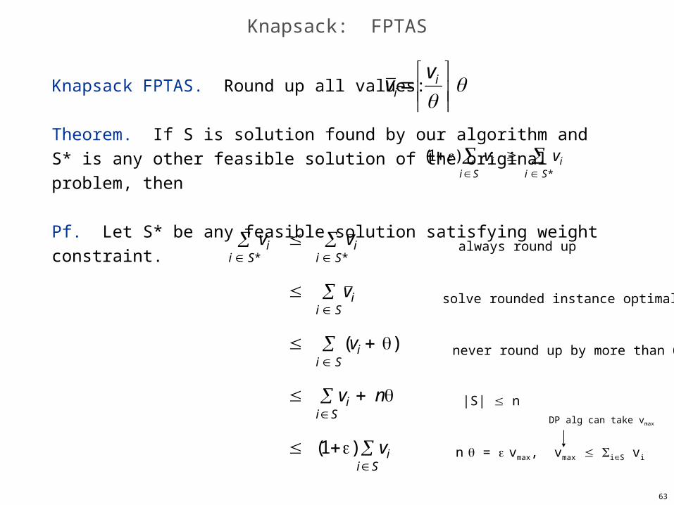
Knapsack FPTAS. Round up all values:
Theorem. If S is solution found by our algorithm and S* is any other feasible solution of the original problem, then
Pf. Let S* be any feasible solution satisfying weight constraint.
vii S* v i
i S*
v ii S
(vii S )
vii S n
(1) vii S
always round up
solve rounded instance optimally
never round up by more than
(1) vi vii S*
i S
|S| n
n = vmax, vmax iS vi
DP alg can take vmax
i
i
vv