A system where at least one component has

dimensions in the range 1 nm-1 (10) µm

What is a colloid?

Dispersed phase(dispersoid)

Continuous phase, (dispersion medium)

A structureless continuum on thelength scale of the dispersed phase

Size (nm)1 10 100 1000 10000

Molecularsolutions

Visiblephases

Colloids

Ostwald: Welt der vernachlässigten Dimensionen

’World of neglected dimensions’

Then: Colloid scienceNow: Nanoscience

Types of disperse systems

Colloidal dispersion

1 nm – ~1 µm

dispersion

Coagulation,flocculation

condensation,aggregation

Heterogenous

dispersion

> 1-10 µm

Heterogenous systems

(blood, milk)

Microheterogenous systems (plasma, macromolecular

solutions)

True solution

< 1 nm

Homogenous systems (salts, acid and base solutions)

dissolution

Dispersed phases

Continuous

Dispersedphase Name Example

Gas Liquid Aerosol Cloud, fog

Solid Aerosol Smoke, dust, pollen

Liquid Gas Foam Beer, bread

Liquid Emulsion Milk, mayonnaise, paper pulp

Solid Sol, suspension Ink, paint

Solid Gas Solid foam Styrofoam, suofflé

Liquid Solid emulsion Butter

Solid Solid sol, suspension Concrete

Air, liquid,

blood…

Bacteria,

viruses, cells…

Most are lyophobiccolloids! Classes

• Colloidal dispersions• Association colloids• Macromolecular solutions

Important differences betweencolloids and true solutions

• Optical properties• Rheology• Kinetic properties• System stability• (Colligative properties, i.e.

concentration dependent)

What colloids are there?

• Lyophobic (’solvent hating’)• Lyophilic (’solvent loving’)

Important areas of study in colloidal systems

• Particle size and shape• Surface properties• Particle-particle interaction• Particle-solvent interaction• Colloidal stability

Colloidal

dispersions

Association colloids

(aggregates of

amphiphiles)

Macromolecular

solutions

d

Thermodynamicallyunstable two-phase systems; subject to Ostwald ripening.

One continuous phase+ dispersed phase(s)

(Suspension if d > 1 µm,dispersion if d < 1 µm )

Thermodynamically stable(one-phase system)

Aggregates 1 nm-1 µm

Structures emerging in solutions of amphiphiles

Thermodynamicallystable (one-phase system)

Macromolecules1 nm-1 µm

One continuous phase +dissolved substance(s)

Lyophilic (’solvent-loving’) colloids

o High affinity to the solvent, usually strongly hydrated

o Can be easily redispersed after drying merely by adding solvent

o No distinct interface with the medium

o Form very stable solutions (lyophilic sols)

o Examples: Proteins, polysaccharides

Lyophobic (’solvent-hating’) colloids

o Interacting weakly with the solvent

o Can be redispersed only after vigorous mechanical agitation after drying

o Form thermodynamically unstable dispersions

o Examples: Metal nanoparticles

Monodisperse Polydisperse

Macromolecular properties

ii

iii

rMn

MMnM

=

)(

Weight averages

Size and shape are important parameters!

Macromolecularradius

R?

A historical example:Classification of bacteria

Three primary bacterial forms:coccus - sphericalbacillus – rod-likespirillum – spiral

Was importantfor speciesidentification!

Other methods:- Colony structure- Staining- DNA/RNA

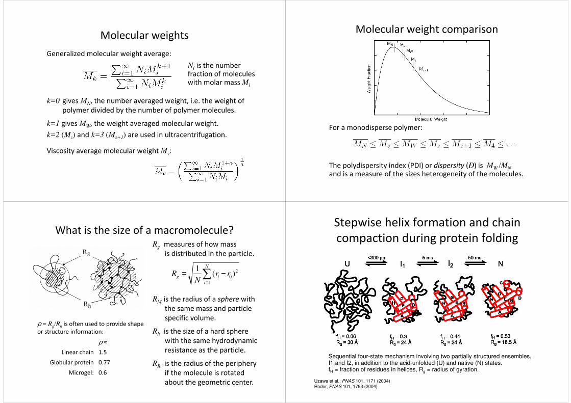
Molecular weights

Generalized molecular weight average:

k=0 gives MN, the number averaged weight, i.e. the weight of polymer divided by the number of polymer molecules.

k=1 gives MW, the weight averaged molecular weight.

k=2 (Mz) and k=3 (Mz+1) are used in ultracentrifugation.

Viscosity average molecular weight Mv:

Ni is the number fraction of molecules with molar mass Mi

Molecular weight comparison

For a monodisperse polymer:

The polydispersity index (PDI) or dispersity (Ð) is MW /MN

and is a measure of the sizes heterogeneity of the molecules.

What is the size of a macromolecule?

ρ = Rg/Rh is often used to provide shape or structure information:

Rg measures of how massis distributed in the particle.

RM is the radius of a sphere withthe same mass and particlespecific volume.

Rh is the size of a hard spherewith the same hydrodynamicresistance as the particle.

RR is the radius of the peripheryif the molecule is rotated about the geometric center.

2

0

1

1( )

N

g i

i

R r rN =

= −

ρ ≈Linear chain 1.5

Globular protein 0.77

Microgel: 0.6

Sequential four-state mechanism involving two partially structured ensembles, I1 and I2, in addition to the acid-unfolded (U) and native (N) states. fH = fraction of residues in helices, Rg = radius of gyration.

Stepwise helix formation and chain compaction during protein folding

Uzawa et al., PNAS 101, 1171 (2004)Roder, PNAS 101, 1793 (2004)

When is a colloid dilute?

Colloids are often assumed to be ’dilute’ to make theoretical treatment easier. When is a colloid dilute?

φ = volume fraction of particlesr = particle radius

φ ≈ 0.02 Multi-particle effects begin to influence dispersion properties

φ = 0.024 Average separation S0 equals particle diameter

φrcp ≈ 0.64 Random close-packing limit

φhcp = 0.74 Hexagonal close-packing limit

The average particle separation (distance between surfaces) is

In reality, most colloidsare not dilute…!

1/3

0 1rcp

S rφφ

= −

Colloid (in)stability

Flocculation → creamingAggregation → creaming

Size disproportionation(Ostwald ripening)

Coalescence

Creaming

Sedimentation

= Reversible

(phoresis)

Methods for determination ofparticle size and shape

1. Study particle motion in a force field(gravitation, centrifugal field)

2. Microscopy (optical, electron or atomicforce microscopy)

3. Study how particles scatter light(light-, X-ray or neutron scattering)

4. Measurements informing about theparticle area (gas adsorption) -

I0

ρ ρ0

Fg

Fb Fν

Kinetic Properties – Brownian motion

• Random and continuous movement of colloidal particles.

• Arises from random collisions the particles and solvent molecules.

• Brownian motion is more rapidfor smaller particles.

• Decreases with increasingviscosity of the medium. = mean square displacement

t = time interval between ’steps’

2l

l

2

6

lD

t= (in 3D)

- Particles diffuse spontaneously from regions of high concentration to regions with low concentration until the system is uniform throughout.

- An immediate consequence of Brownian motion.

- Fick's first law describes the diffusion:

Kinetic Properties – Diffusion

cJ D

x

∂= −∂

[mol/m2 s]

The diffusion coefficient D [m2/s] is the amount of materialdiffused per unit time across a unit area when dc/dx is unity.

Can be used to determine particle radii, or molecular weights!

The sedimentation velocity is given by Stokes‘ Law:

Vs = rate of sedimentationd = diameter of particlesρ = density of internal and external phasesg = gravitational constantη = viscosity of medium

Kinetic Properties – Sedimentation

2 ( )

18i e

s

d gV

ρ ρη−=

Microscopy

Resolution: δ = λ / 2n sinθ(”diffraction limit”)

λ wavelengthn refractive index

For visible light, the maximum resolution is d ~ 200 nm at best

- Cannot distinguish features of colloidal particles.- Reduce λ (or increase n) to improve resolution?- Weak contrast between particles and surrounding medium

may reduce visibility even for large particles (cells…).

Other options: Darkfield- or ultramicroscpyElectron microscopyScanning probe microscopy

Optical microscopy

Darkfield- and ultramicroscopy• Increases contrast by illuminating the sample from

the sides, so that only light scattered from particles is visible (the Tyndall effect).

• Increases contrast; 5-10 nm metal particles can be observed, for materials with lower refractive index ~ 50 nm particles.

• Irregular particles give variations in the scatteredlight as they tumble through the solution, whilespherical particles give constant scattering.

• Useful for studies of e.g. Brownian motion, particlevolume, or particle shape.

Wavelength-dependentscattering from silvernanoparticles underdarkfield illumination.

Super-resolution microscopy

Hell et al., Current Opinion inNeurobiology 2004, 14:599–609

Stimulated emission depletion (STED)

Stochastic Optical Reconstruction Microscopy (STORM)

Structured Illumination Microscopy (SIM)

Optical microscopy vs. TEM(Transmission electron microscopy)

λ ~ 10-12 mResolution ~ 0.2 nmRequires vacuum, ~ 10-6 torrThin samples, ~ 250 nmParticles from 1 nm – 5 µm

Opticalmicroscope

Electronmicroscope

λ ~ 10-7 m

Resolution ~ 0.2 µm

13 nm

Gold nano-particles, TEM

(Daniel Aili, IFM)

Cryo-TEM

By vitrification of liquids(water), structure in organicmaterial can be retained afterfreezing and subject to TEM investigation!

(Vesicles formed from a detergent.)

SEM(Scanning electron microscope)

An electron beam is swept over the sample, and emitted electrons arerecorded; the intensity variationsare used to build a topographic image.

Resolution ~ 5 nmRequires vacuum (not E-SEM)Huge depth of focus!

This is how theimage is perceived!

(Spores of the alga U. lactuca)

Atomic force microscopy (AFM)

A small tip is swept over the surface and its deflection (which is assumed to relate to topography) is registered.

Methods for ”imaging” of surfaceswhere a probe is swept across a surface to provide a map of somesurface property.

Probes can be sensitive to topography, elasticity, electron density, surfacecharge, heat conductivity, chemicalinteractions (ex. acid-base), biorecognition events (ex. base pairs), magnetism etc.

Magnetic image ofthe surface of a HD

Topographic imageof a DVD-master

Scanning probe microscopy, SPM

With an applied potential between thetip and the surface, a current will flowacross the gap at < 1 nm separations.

This tunneling current can be usedto extract topographicalinformation.

Requires electricallyconducting samples.

(What is really measured is the density of filled or emptyelectron states at the surface, depending on the polarity ofthe applied potential.)

~

Scanning tunneling microscopy, STM

SNOM(Scanning near-field optical microscopy)

By leading light through a tapered opticalfiber with a 50-100 nm opening, and thendetect the light which is either

• reflected back into the fiber, or

• transmitted through the sample

Optical images with ~20 nm resolution areobtained!

– 10 times better than optical microscopy!

The method uses the evanescent field outsidethe fiber end, equivalent to tunneling of lightthrough the narrow aperture!

SNOM-example(http://snom.omicron.de/)

500 nm particles (PS)

Optical

microscopy

2 µm 5 µm

Reflection Transmission

SNOM

Light scattering

• Visible light, X-rays or neutrons

• The intensity distribution at varying angles

contains information about particle size, shape,

internal structure and thermodynamic properties.

Scattering vector

(or Momentum transfer)

Light is scatteredagainst inhomoge-neities in medium

4 sin( / 2)q q

π θλ

= =

Laser Sample

Detector

θq

TurbidityTurbidity τ is defined by It / I0 = e -τ l

and is a measure of the scattering capacity.

For small molecular weightsthe scattered intensity I isindependent of q, and

I0l

It

I is proportional to c × M

c = concentration,M = molecular weight.

Turbidimeter: primitive light scattering meter.

Tyndall effect

Storleksområden i ljusspridning

Dynamic light scattering

• DLS – Dynamic Light Scattering,

PCS – Photon Correlation Spectroscopy

QELS – Quasi-Elastic Light Scattering

• Fluctuations in the scattering at a fixed angle result from diffusion of particles into and out of the illuminated volume.

• Provides dynamic information (diffusion coefficient D) about the particles, from which the size is obtained via the hydrodynamic radius Rh in Stokes-Einstein’s ekvation:

6B

h

k TD

Rπη=

Dynamic light scattering Intensity fluctuations I(t) are measured directly, and the (intensity)autocorrelation function g(t) is calculated. The diffusion constantis obtained from the time correlation function g´(t) = g(t)-1 :

2

2

( ) ( )( ) 1

( )

q DI t I t

g eI t

τττ β −+

= = +

ln g´(t) for Oxyhemoglobin,The slope Γ is –q2D

´

DLS example: 700 kDa PVP

Intensity fluctuations I(t) are measured directly, and theautocorrelation function is calculated, from which the diffusionconstant is obtained:

-4

-3.5

-3

-2.5

-2

-1.5

-1

-0.5

0

0.00 0.20 0.40 0.60 0.80

τ (ms)

ln g

1( τ

)

0

0.1

0.2

0.3

0.4

0.5

0.6

0.7

0.8

0.9

1

1E-04 0.001 0.01 0.1 1 10 100

t (ms)

g1(t

)

Deviation indicating polydispersity

From the slope G:

Rh = 23 nm

Static light scattering

• Measure the absolute intensity I = I(c, θ ) of the scattered light.

• Reference measurements are required:a) A standard for which the absolute scattering is

known (e.g. toluene, benzene).b) The solvent in which the scatterers are dispersed/dissolved.

• Provides thermodynamic information:Molecular weight average Mw

The radius of gyration Rg

The second virial coefficient A2

• Rayleigh scattering (d << l) Particles scatter light as pointsources.

• Debye scattering Large particles, but low contrast (for visiblelight, d ~ 10-100 nm), e.g. vesicles, PEG, proteins.

• Mie scattering (d > l) Each scatterer is large enough to givephase differences in light scattered in one direction, resultingin interference, giving strong angular dependence.

Size dependence (1st approximation)

~

Rayleigh scattering

Particles are small enough to be evenly illuminated by coherentlight in the same phase. Then:

Iθ = Scattered intensity in direction θα = Particle polarizabilityΝ = Number density

( )2 4

2

2 4

0

81 cos

IN

I r

θ π α θλ

= +

I0

Polarisation:HorisontalVerticalUnpolarised

Mie scattering

Each particle is large enough to cause interference in the lightscattered from itself, i.e. the scattered light will have maximaand minima as the scattering angle changes.

At θ = 0 there is no interference, and if data is extrapolated to θ =

0 and c = 0, application of the Rayleigh theory is much easier.

→ Zimm-plot

Molecular weights from scattering experiments

Rayleigh-scattering: Scattering ∝ cM ∝ Rq

Debye scattering: 1

2Kc

BcR Mθ

= +

1 12

KcBc

R P Mθ θ

= + Mie scattering:

00

1limc

Kc

R Mθθ→→

=

Extrapolate to 0° andc = 0 in a Zimm-plot.

K(n,n0,λ,c) andB are constants

4 2

4

8Rθ

π αλ

=

Pθ form factor

Particle surface charge (zeta-potential)Light scattering and the zetasizer

Two intersecting laser beams create an interference pattern. A charged particleis ”dragged” through this pattern by and applied field, giving fluctuations in the scattered light. The frequency of these fluctuations depend on the particlevelocity, which in turn depend on the surface charge.

Malvern ZetaSizer

X-ray- and neutron scatteringSAXS/SANS

(Small-angle x-ray/neutron scattering)

• The same optical principles as for visible light, butthe wavelengths and the contrast mechanismsare different.

• Neutrons: Weak intensity, but good contrastbetween different atoms. λ ~ 1-10 Å.

• X-rays: High intensit, but weak contrast betweendifferent atoms (electron density), λ ~ 1-10 Å

Interlude: Contrast variation for the determinationof a glass refractive index

Vary the refractive index of the liquid until the glass rods “disappear”

n = 1.45 n = 1.47 n = 1.50

Example: Composition of mixed micelles(R.K. Thomas, Oxford)

Problem: In a solution of two surfactants, determinethe composition of the mixed micelles.

Solution: Use neutron scattering, and use the difference in contrast between protonated (1H) and deuterated (2H=D) hydrocarbon chains.

”Label” one surfactant with deuterium, then varythe H/D-ratio in the surrounding water until the micelles become invisible.

Varying the solvent contrast (H2O/D2O ratio) to determinethe composition of a mixed micelle (C12E6/C16TAB)

The total scattering is smallest when the hydrogen/deuteriumratio of the micelles and the solvent are equal.

Integrate allintensities

Varying the solvent contrast (H2O/D2O ratio) to determinethe composition of a mixed micelle (C12E6/C16TAB)

Plot the integrated scattered intensities versus the solvent composition, and obtain the micelle composition from the

zero crossover.

Osmosis Equilibrium between two solutions of different concentrations separated by a semi-permeable membrane occurs when:

• the substance is distributed equally – if the membrane is permeable.

• the solvent has moved to equalize the difference – if the membrane is semi-permeable.

Osmotic pressure: the pressure applied against the transfer of solvents through the membrane

Osmotic pressure• Proportional to the concentration of dissolved

particles (regardless of size) – a colligative property.

• Ionizable substances - participate in the osmotic pressure alone

p = iRTc

The values of the coefficient i depends on the nature of the substance and its concentration

– Non-dissociated particles → i = 1– Univalent salts (KCl, NaCl, KNO3) → i = 2– Uni-divalent salts (K2(SO)4, CaCl2) → i = 3– Uni-trivalent salts (AlCl3, K3Fe(CN)6) → i = 4

Osmotic pressure in colloidal dispersions = oncotic pressure

i = number of ionized particlesc = concentration

Osmotic pressure

Osmoregulation is the homeostasis mechanism of an organism to reach balance in osmotic pressure.

o Hypertonicity is the presence of a solution that causes cells to shrink.

o Hypotonicity is the presence of a solution that causes cells to swell.

o Isotonicity is the presence of a solution that produces no change in cell volume.

Osmotic concentration(formerly ’osmolarity’)

The osmotic concentration determines the osmotic pressure, and is defined as the number of osmoles (Osm or osmol) of the solute per liter of solution.

Osmolarity differs from molarity in that it measures particle, rather than solute, concentration, thus taking dissociation into account.

Salts dissociate, and both ions affect the osmotic pressure:

1 mole of NaCl in solution ⇔ 2 osmoles of solute particles1 mol/l NaCl solution ⇔ 2 Osm/l NaCl solution

Viscosity = Resistance to flow of a system under applied stress. The more viscous a liquid, the greater the applied force required to make it flow at a particular rate.

The viscosity of a colloidal dispersion is affected by the shape of particles of the disperse phase:

Spherocolloids dispersions of low viscosity

Linear particles more viscous dispersions

Kinetic Properties – Viscosity

0 (1 )kµ µ φ= +

In dilute solutions ( < 0.02), the viscosity is given by:

µ0 = medium viscosityk = constant (2.5 for spheres)

Non-Newtonian liquids

Shea

r st

ress

, τ(P

a)

Shear rate, γ’ (1/s)

Newtonian liquid: viscosity is constant under shear (flow).

Shear thinning liquids:Ketchup, blood, latex paints

Shear thickening liquids:Suspensions of starch in water

Bingham plastics:Toothpaste, mayonnaise