Distributed Computing

What’s it worth?

Semester Thesis

Robert Strietzel

strrober@ethz.ch

Distributed Computing Group

Computer Engineering and Networks Laboratory

ETH Zurich

Supervisors:

Philipp Brandes, Pascal Bissig

Prof. Dr. Roger Wattenhofer

July 4, 2013

Contents

1 Introduction 1

2 Related Work 2

3 Fetching the data 3

3.1 Finding Objects . . . . . . . . . . . . . . . . . . . . . . . . . . . . 4

3.2 Extracting useful information . . . . . . . . . . . . . . . . . . . . 4

3.3 Bad Data . . . . . . . . . . . . . . . . . . . . . . . . . . . . . . . 5

4 Creating the Model 7

4.1 Parameters . . . . . . . . . . . . . . . . . . . . . . . . . . . . . . 7

4.1.1 Size . . . . . . . . . . . . . . . . . . . . . . . . . . . . . . 8

4.1.2 Geoinformation . . . . . . . . . . . . . . . . . . . . . . . . 9

4.1.3 Age . . . . . . . . . . . . . . . . . . . . . . . . . . . . . . 11

4.1.4 Floor . . . . . . . . . . . . . . . . . . . . . . . . . . . . . 13

4.1.5 Binary Parameters . . . . . . . . . . . . . . . . . . . . . . 13

4.2 Models . . . . . . . . . . . . . . . . . . . . . . . . . . . . . . . . . 16

4.2.1 Absolute Model . . . . . . . . . . . . . . . . . . . . . . . . 16

4.2.2 Relative Model . . . . . . . . . . . . . . . . . . . . . . . . 16

4.3 Overfitting/Boundaries . . . . . . . . . . . . . . . . . . . . . . . . 17

5 Results 18

Bibliography 21

i

Chapter 1

Introduction

Finding an apartment today is easier than ever. Instead of looking on the streetsor canvass different estate agents we can just go online and start searching forsomething suitable in the thousands of offers on different websites. After a whileyou may get an idea, which one might be a good offer and which one is not,however as every apartment is different it is hard to compare them. There aremany factors which influence the price of a house or a flat, such as the size,location or age.

First of all it is a market which is driven by demand and supply. The pricesin areas with high demand and limited supply, for example in city centres, aremuch higher than in areas with low demand and high supply. Apart from thelocation there are many other factors the price depends on. Houses are thereforea very heterogeneous good. The price of a commodity is then a function of allthese factors. This is called hedonic pricing[1].

Estimating the composition of the price has been a topic of interest for manyresearchers and businesses. This information is valuable for property owners andreal estate companies because they wish to know for which price they can rentout their property. On the other hand this information is also valuable for peoplesearching for a flat to be able to check whether the price is justified. A thirdgroup are researchers in the economic and social sciences as societal values anddevelopments can be derived from such information.

This semester thesis attempts to model this composition and the value of itsdifferent parameters for Switzerland using offers, which are publicly available inthe Internet.

First all offers from a large platform for flat renting are fetched. Afterwardsthese offers are searched for any information which can have an influence onthe price of this offer. If a piece of information has a sufficient frequency to bestatistically relevant it is used as a ’feature’. In a next step the value of thesefeatures are computed using different models. Finally these models and valuesare assessed.

1

Chapter 2

Related Work

A lot of research has been made on the prices of real estate and private rentedsector. However, these studies and articles focus on smaller regions or cities,such as Hong Kong [2], Bordeaux [3], Tokyo [4] or Los Angeles [5]. The pricewas hereby always modelled using the hedonic approach with different parame-ters. To fit the data in the model usually the Linear Least Squares Regressionwas used. One article however compared different algorithms and could achieveslightly better results using a spatial autoregressive error model which takesregional dependencies into account.

The Linear Least Squares Regression implies that each parameter has anabsolute price. This assumption shall be scrutinized in this paper by comparingit with a model in which the prices of the parameters are location-dependent.

Essentially two types of parameters can be distinguished. The first group areparameters based on the location of the object. This can for instance includedistances to the city centre, to the next train station or the next supermarketas well as properties of the neighbourhood such as the air quality. The secondgroup of parameters are properties of the flat itself. Important ones are usuallythe size and the floor of the flat followed by the facilities which differ significantlyamongst different areas. In Tokyo for example an important factor is whetherthe house is build of reinforced concrete[4] whereas in Bordeaux balconies andthe number of bathrooms are important[3].

As these studies all cover a rather small area, their sample size is also rathersmall, ranging from 150 to 1000 samples. This thesis however tries to find amodel which is more general and covers a whole country. To be able to takeregional differences into account as well, a greater number of samples is needed.

2

Chapter 3

Fetching the data

Renting contracts are not publicly viewable and there is no public databasewhich contains prices and features of all flats in Switzerland. What can befound are offers for flats which are advertised for renting. These advertisementscan be found at different locations: Signs on the street, public pin-boards, real-estate agents or in the internet. To be able to achieve robust results usingregression methods a big dataset is required as there is a great variety of possiblecombinations of attributes, especially if the location is seen as an attribute aswell.

This is only achievable using the offers from internet portals. Fortunatelythere are a few websites with several thousand offers for apartments. For Switzer-land these are Comparis 1, Homegate 2 and Immoscout24 3 The database of the-ses websites is not public and there is also no public API to retrieve the offers.The obvious way therefore is to scan one or more of these website and extractthe offers from the HTML pages.

For this thesis data from Immoscout24 was used since this is one of the portalswith the highest number of objects and it does not forbid crawling the website.

Crawling Websites is fairly simple today as several libraries and packages fordifferent programming languages exist to simplify the process. For this projectthe Python library Scrapy 4 was used. It is capable of queuing requests andpause a certain time between them because a large number of request in a shorttime can be seen as a denial of service attack.

1https://www.comparis.ch/immobilien/default.aspx2http://www.homegate.ch/3http://www.immoscout24.ch4http://doc.scrapy.org/en/0.16/

3

3. Fetching the data 4

3.1 Finding Objects

Each Object can be fetched by using the ObjectID. Unfortunately this numberis not simply counting up so we could loop over all numbers. Therefore it isnecessary to extract these IDs from an object listing. As it is not possible to listall objects in Switzerland an iteration through the cantons, which is the highestlevel available, needs to be done. Normally only 30 items are displayed on eachpage, which leads to a high number of request by iterating through all pages of acanton. Conveniently the number of items on a page can be increased by addinga cookie to the request which leads to a significantly reduced amount of requests.

3.2 Extracting useful information

The information about the offer is just a small part of the HTML-Page, whichwas downloaded. It is therefore necessary to find and extract the pieces ofinformation we are interested in and eliminate layout and formatting of thispart.

Some features such as the price, the size and the address of an object arealways at the same location of the website. This data can therefore be easilygathered using the XPATH 5, which uniquely defines a content element on awebsite.

This is however not the case for most of the other features of a flat, suchas balconies, parking space and other elements of the interior. This informationcan either be found in the standardized list the portal provides or in the textdescription. In this case a more flexible way of gathering information is necessary.The fact that normally nobody writes down features, which are not available,makes this easy as we only need to search whether certain features such as’balcony’ or ’dishwasher’ occur somewhere in the text. However, this only worksto determine whether a certain feature exists or not. The amount of this item(e.g. the number of balconies) and whether this item costs extra (this is oftenthe case for garages or parking space) cannot be determined as easily.

We only want to gather features, which are statistically relevant. Thus thefirst step is to analyse which words appear how often in the offers. An extractof this list, sorted by the number of occurrences in descending order is shown inFigure 3.1. In a second step the words, which actually contain a feature of a flatneed to be separated from the words which are not useful.

5http://www.w3.org/TR/xpath

3. Fetching the data 5

Figure 3.1: Frequency of words in the description of offers

3.3 Bad Data

When fetching data automated from the internet it is inevitable that some objectsviolate the predefined pattern or have incomplete or wrong information supplied.These object can distort the results of the analysis dramatically. This is mainlycaused by the fact that the price level of an area is based on the surroundingoffers which means that one wrong offer can bias the price level of a whole area.Finding and eliminating these objects is therefore important to obtain meaningfulresults. Basically there are two types of objects which must be eliminated:

The first type are objects where not enough data is supplied. There areseveral offers with price ’on request’ which naturally cannot be used in the model.As seen before the location and the size are also crucial parameters and objectsnot containing one of them can therefore not be used. The Google API is howeververy flexible, hence also incomplete addresses may be used as long as they canbe tracked to geographic coordinates by the API.

The second type are object with obviously wrong information. The mostcommon case is that the price is not given per month, which is the standard onall big property portals but per week, day or year. Another commonly mistakenlyused field is the size. Here again it makes sense to use the price per squaremeteras filtering variable because first the spread between a small and big flat canbe higher than the difference between monthly and weekly price and secondlybecause we can combine the two mistakes to a common exclusion criteria. Ofcourse it is not possible to filter all incorrect offers with this method but atleast the ones with the highest influence on the model can be eliminated. After

3. Fetching the data 6

manual examination of offers with very high or very low price per squaremeterthe flats with a squaremeterprice below 6CHF/m2 or above 120CHF/m2 arealways mistakes and can therefore be excluded.

Chapter 4

Creating the Model

As previously mentioned, the flat as a heterogeneous good includes numerousimplicit features. The price of the flat can then be written as a function of thesefeatures. The simplest function, which also is the standard for hedonic pricing, isthe sum of the features. Different features possess different values. Thus, everyaddend has a coefficient describing this value. These values can then calculatedbased on the statistical data using numerical methods. Before composing thisfunction the different parameters which have an influence on the price and theirproperties should be considered.

4.1 Parameters

Generally every piece of information from an offer, which has an influence on theprice, can be seen as a parameter of the function describing the total price of aflat.

There are different types of parameters. The simplest type is a binary pa-rameter. This means that a feature, for example a lift or a dishwasher, is eitherexistent or not.

The second type is a simple numeric parameter. Examples are the size andthe year the flat was build. For these parameters a function needs to be found,which maps the change of the parameter to a change in the price. Alternativelyvalues of this parameter can be grouped and then these groups can be handledas binary parameters.

Finally there is the location as a more complex parameter. The location isgiven as an address which can not be used in a mathematical model withoutpreprocessing. For this parameter methods need to be found to convert theaddress to a single numeric value which can be used in the model.

7

4. Creating the Model 8

4.1.1 Size

The size of a flat is one of the first filters available on every real estate portal.The size therefore seems to be an important feature of a flat or house.

In previous studies there were two different approaches to model the rela-tionship between the size and the price of flat. Most model the size in a linearmanner meaning that the share of the final price, which is solely based on the sizeof the flat, is twice as high if the size is doubled. Other work used a logarithmicapproach for this relationship. This means that the added value for added spaceis not fixed but decreases with rising size.

To determine which model fits to flats in Switzerland the relationship betweenthe size and the price of the flats is plotted in Figure 4.1 in green. The trendthat with rising size the price increases is already visible but as this is not theonly important factor the spread is quite high.

Better results can be achieved by only selecting offers for a specific regionto reduce price differences between them. Zurich is well known for its high flatprices and can thus be taken as one example. The red dots in Figure 4.1 are theoffers located in Zurich. In this case a linear correlation seems to fit well to thepoints and the spread is significantly lower. A decrease in the slope with risingsize cannot be confirmed.

Figure 4.1: Price of flats in Zurich compared to Switzerland

4. Creating the Model 9

4.1.2 Geoinformation

It is commonly known that a flat in the centre of a city is much more expensivethan a comparable flat in the countryside. The location is therefore one of thefactors with the highest influence. The plain address as string however containsno direct information about the value of this location. A first approach to verifythe assumption of the value of the location to use the postcode to distinguishbetween high- and low-price areas. In figure 4.1 all offers which are located inthe postal code areas of the city of Zurich are coloured red whereas all othersare green for different sizes of the flat. It is observable, that flats in Zurich arealmost twice as expensive as the average regardless of the size.

Also visible in Figure 4.1 is that the price in an area rises approximatelylinear with the size of the flat. It is therefore more feasible to use the price persquaremeter as an indicator for the price level of an area.

As postcodes comprise quite large areas and thus can contain also differentprice levels a more accurate estimation for price areas is needed. For this theprecise position of the object is required first. Several APIs are available toconvert an address to geographic coordinates. In a small number of samples theGoogle Geocoding API 1 could map the most addresses to the right coordinatesand was therefore used for this thesis.

The next step is to determine the price level of certain areas. The easiestway would be to define a grid with a certain block size and find the average pricelevels for every frame of the grid based on the objects in this area. The problemwith this approach however is that houses, especially in Switzerland, are veryunevenly distributed over the country. This would result in many frames withno or only a few objects and some frames with a very high number of objects,where also large price level differences inside of this frame are possible.

In order to obtain a meaningful price level for a location rather a certainnumber of the closest objects should be used regardless of their distance to thislocation. Again a trade off between the resolution of the price areas and agood average of an area has to be found by choosing an adequate number ofsurrounding objects for the calculation of the average price level at this location.

The optimal number of surrounding objects can be found by comparing theaverage absolute difference between the real price per squaremeter and the av-erage price per squaremeter based on each number of neighbours. The result isvisualized in Figure 4.2 The number for which this average difference is minimalis the optimum. In our dataset with around 20000 entries this optimal numberis 27.

1https://developers.google.com/maps/documentation/geocoding/?hl=en

4. Creating the Model 10

Figure 4.2: Price level in Switzerland

In Figure 4.3 the price levels of all objects are plotted on their geographicposition. The big cities of Switzerland as well as the unequal geographic distri-bution are clearly visible.

Figure 4.3: Price level in Switzerland

4. Creating the Model 11

4.1.3 Age

Intuitively the newest flats are the most expensive ones. However there is nolinear trend that the value decreases with increasing age as visible in Figure 4.4and 4.5. In these plots the difference between the real price and the product ofsize and the above calculated price per squaremeter in this area is calculated forevery offer of the respective year. The box contains the middle 50 percent of thedata and the line in the box represents the median of them. The whiskers showthe total range of the data. In Figure 4.4 an extract of the first 53 years areshown. In Figure 4.5 the age is aggregated in groups of 5 years in order to showa wider range of years and have more significant boxes at higher ages where lesssamples exist.

One way to handle this non-linear age dependency would be to fit a curvein the graph and add this function to the optimization. This only works wellif there is no or only little influence from other parameters. This is not thecase with our model though. Many parameters are heavily age-dependent, fora example Minergie houses are mostly very new and flats with parquet flooringtend to be older ones. If these parameters are added the shape of the graphmight change. Another problem with this approach is as noted before that thenumber of samples is decreases strongly with higher age.

4. Creating the Model 12

Fig

ure

4.4:

Pri

ced

evia

tion

for

diff

eren

tag

es

Fig

ure

4.5:

Pri

ced

evia

tion

for

diff

eren

tag

esin

grou

ps

offi

veye

ars

4. Creating the Model 13

A second, more suitable approach therefore is to group several years withsimilar value and handle these groups as binary parameters. The size of thesegroups can then be adjusted to the number of samples which leads to more yearsgrouped together with rising age. Based on these plots the following groups havebeen formed: 1955-1977, 1978-1992, 1993-2005, 2006-2009, 2010-2013

4.1.4 Floor

To see whether the floor has an influence on the the price the difference betweenreal price and the price estimation based on location and size is again shown asa box-plot in Figure 4.6. This relationship is clearly not linear and has to behandled in another way. As the number of samples for floors higher than five iscomparatively low with a very high spread these floors can be discarded. Theremaining six floors (0-5) can then be used as binary parameters.

Figure 4.6: Price deviation for different floors

4.1.5 Binary Parameters

The remaining features are either existent or not. If one of the keywords ex-ists in the description the variable is one and otherwise it is zero. In order toverify results from the regression the impact of each of the feature was assessedseparately.

This can be done by comparing the difference between the real price and theprice based on location and size of the flats ∆P which have this feature with

4. Creating the Model 14

the ones without it. In Figure 4.7 these deviations are plotted as a histogram inthe background. Subsequently it is possible to fit a normal distribution in thishistogram. These are visualized in the foreground of Figure 4.7. The parametersof these fits can then be compared to determine the impact of this feature. If theaverage value of the fits are very close to each other this feature is probably notvery important, whereas if they differ substantially it has a high influence. Forthe parameter ’Minergie’ we can see from Figure 4.7 that a flat containing thisfeature is on average more than 200 CHF more expensive than a flat without it.

Figure 4.7: Price deviation for different floors

However not only the difference of the average value ∆P of the plot plays arole when comparing the similarity of two standard deviations. A standard dis-tribution also contains the variance as a parameter which should be considered.If the parameter contains a lot of noise, leading to a high variance, a differencein the average value is probably not as meaningful as if the variance is verylow and there is only little noise. However, if the features should be ranked byimportance it is necessary to combine these two parameters to single one. Oneway to do this is to use Equation 4.1 which is also used by the Fisher LinearDiscriminant to find the best baseline for a standard distribution in two groupsof more dimensional points.[6]

J =|µ1 − µ2|2

σ21 + σ22(4.1)

This can be calculated for all parameters to be able to rank them by im-portance. The results can be found in Table 4.1. This ranking is needed ifit is necessary to reduce the number of parameters in case the dataset is not

4. Creating the Model 15

Parameter JF isher ∆P

minergie 0.100 999 372 1 214.367 106 195 5wheelchair 0.028 323 360 8 120.569 055 125 2floor heating 0.015 383 751 4 89.369 856 696 4washer 0.013 941 842 3 83.945 497 939 9stone floor 0.012 354 550 6 74.378 741 316 5Floor 0 0.008 635 527 2 58.754 661 985 8dishwasher 0.006 377 649 4 54.239 046 55lift 0.004 195 85 45.759 608 358 9Floor 3 0.001 250 259 5 24.322 405 835 1central heating 0.001 232 014 9 −22.055 87laminat 0.001 170 909 2 −20.395 990 078Balcony 0.000 905 383 −21.422 735 631 2Floor 2 0.000 744 504 3 −17.901 910 247 7shower 0.000 549 647 4 −16.662 084 261 9view 0.000 196 286 9 −10.536 585 287 8Floor 1 4.550 455× 10−5 4.435 31parking 3.146 036× 10−5 3.951 02parkett 0.000 026 067 −3.373 302 421

Table 4.1: Siginificance of Parameters

large enough to have meaningful results using all of them. The difference of theaverage can then also be used to verify the results of the regression.

Some values may seem counter-intuitive in the first place. One example is thenegative ∆P for balcony, which might imply that balconies decrease the value ofa flat. As this analysis ignores the value of other parameters this implication isnot right. Balconies for example can not be found in the ground floor and as wecan see in the same table the ground floor has a quite high value. Values withbalconies are therefore mainly compared with flats in the ground floor which aremostly more expensive.

This verification can however only be done in a qualitative way because someof the parameters are not linear independent. If a parameter is therefore as-sessed separately the difference in the average value can contain parts of otherparameters which correlate with this one. An example is that all Minergie housesare most likely new as this standard is very new. As we have both the age andthe Minergie feature in the regression the value of the separate inspection willinclude also values from other parameters which correlate with this one.

4. Creating the Model 16

4.2 Models

4.2.1 Absolute Model

If the linear model described previously is used the function of the price P is asum of the properties of the flat xi multiplied with their respective coefficientsai

P =

n∑i=1

aixi (4.2)

This requires that all properties are linear. Most of the parameters are now in abinary form which can directly be used in a linear model. The only two parame-ters which are not binary are the size and the location. As confirmed before thesize can be modelled as a linear parameter. However, the coefficient calculatedwhen using it as such would be the price per squaremeter which we know isdifferent for different areas. To be able to have a common coefficient for all areaswe therefore need to first multiply the size with the price per squaremeter forthis area. Consequently we already have included the only non-linear parameterin the model. The coefficient calculated now is simply the share of the final pricewhich is based on the size and the location of a flat. The coefficients of the otherparameters are then the absolute value in CHF of the respective feature.

If the Equation 4.2 is now set up for every object in the database an over-determined system of equations is obtained. The coefficients can then be com-puted using the least-squares-method.[7]

4.2.2 Relative Model

Another possibility is that the features do not have an absolute value but insteadincrease the final price by a relative amount. This is only applicable for binaryparameters and not for the size and location. For this a reference is needed. Thisreference is the base price which is the price of the flat without any features. Fromthe previous regression this would be the first addend meaning the product ofthe size S, the average price per squaremeter in this area pavg and the coefficientdefining the share of the final price of this product x1. Using this as a factor forthe binary parameter ai leads to Equation 4.3

P = S · pavg · x1 + S · pavg · x1n∑

i=2

aixi (4.3)

Because this is a non-linear equation the ordinary least-squares algorithmcan not be used here. Instead a iterative algorithm such as the Trust-Region-Reflective Optimization [8] is necessary. As this is an iterative algorithm appro-priate initial coefficients must be chosen. As a flat start x1 was set to 1 and all

4. Creating the Model 17

other coefficient were set to 0. This would mean that the price only depends onthe size and the location of the flat which seems to be a good first estimationfrom the previous realisings. Using different starting values, e.g. setting all xito zero did not change the result. The regression therefore seems to convergenicely with the starting values only having an impact on the number of iterationsnecessary to reach the optimum.

4.3 Overfitting/Boundaries

In the beginning a simple recursion with all parameters lead to high positive andnegative coefficients which did not match at all the outcome of the investiga-tion of the single parameters. A recursion with only a few variables by contrastlead to all positive coefficients which matches the previous findings quite well.This problem is widely known as overfitting [9], which means that there are toomany parameters for a too small dataset. The dataset can then be fitted almostperfectly by the parameters but the results will not describe the underlying rela-tionship. Instead the noise of the data is modelled. Especially if there is a strongcorrelation between parameters these parameters can then not be distinguishedwell enough and it is possible that they eliminate each other by having contrary,very high coefficients.

In order to assess whether overfitting happened the results from the regres-sion can be compared with the individual parameters examined above. Due tothe strong correlation of some parameters it is not possible to compare actualnumbers, but the trends are sufficient to judge the result.

A second way to check for overfitting is cross-validation. The dataset is thenrandomly divided in two groups. One group is then used to train the model.This model is then also applied on the second group. If the residuals of bothgroups are similar distributed no overfitting has occurred.

If overfitting has been observed there are two options for coping with it. Thefirst option is to purge variables, preferably the least significant ones based on theanalysis above. The other option is to introduce boundaries for the variables.From the investigation of the different parameters above it is possible to tellwhether the parameter increases or reduces the price. Most of the variables arefeatures, which should not reduce the value of the object. For these parameterit is possible to set the lower boundary to zero. This helps because it is notpossible that two strongly correlated parameters eliminate each other by havingan opposing sign.

Chapter 5

Results

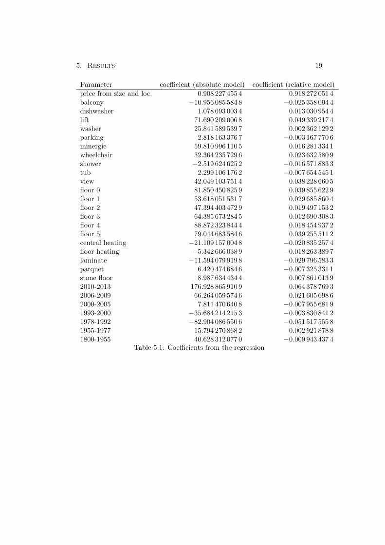
In the end, with about 20’000 usable offers it was not even necessary to introduceboundaries to achieve a meaningful result. This applies for both the model withthe absolute values as well as the model with relative values.

The coefficients determined by the minimisation of the functions of the twomodels can be found in Table 5.1. The coefficients in the absolute model representthe price in CHF whereas the coefficients in the relative model except x1 needto be multiplied with x1, the size and the averaged price per squaremeter in thisarea in order to calculate a price. The latter lies between 15CHF/m2 in ruralareas and 40CHF/m2 in city centres.

The most obvious way to analyse the results of the regression is to look atthe residuals of each row. In this case the residual the difference of the real priceand the price based on the model. In Figure 5.1 and 5.2 the percentage deviationof all objects are shown for the absolute and relative model respectively.

Figure 5.1: Percentage deviation forthe absolute model

Figure 5.2: Percentage deviation forthe relative model

For the cross-validation the data has been randomly divided in a set of 15000samples for training and about 5000 samples for the validation. The distribution

18

5. Results 19

Parameter coefficient (absolute model) coefficient (relative model)

price from size and loc. 0.908 227 455 4 0.918 272 051 4balcony −10.956 085 584 8 −0.025 358 094 4dishwasher 1.078 693 003 4 0.013 030 954 4lift 71.690 209 006 8 0.049 339 217 4washer 25.841 589 539 7 0.002 362 129 2parking 2.818 163 376 7 −0.003 167 770 6minergie 59.810 996 110 5 0.016 281 334 1wheelchair 32.364 235 729 6 0.023 632 580 9shower −2.519 624 625 2 −0.016 571 883 3tub 2.299 106 176 2 −0.007 654 545 1view 42.049 103 751 4 0.038 228 660 5floor 0 81.850 450 825 9 0.039 855 622 9floor 1 53.618 051 531 7 0.029 685 860 4floor 2 47.394 403 472 9 0.019 497 153 2floor 3 64.385 673 284 5 0.012 690 308 3floor 4 88.872 323 844 4 0.018 454 937 2floor 5 79.044 683 584 6 0.039 255 511 2central heating −21.109 157 004 8 −0.020 835 257 4floor heating −5.342 666 038 9 −0.018 263 389 7laminate −11.594 079 919 8 −0.029 796 583 3parquet 6.420 474 684 6 −0.007 325 331 1stone floor 8.987 634 434 4 0.007 861 013 92010-2013 176.928 865 910 9 0.064 378 769 32006-2009 66.264 059 574 6 0.021 605 698 62000-2005 7.811 470 640 8 −0.007 955 681 91993-2000 −35.684 214 215 3 −0.003 830 841 21978-1992 −82.904 086 550 6 −0.051 517 555 81955-1977 15.794 270 868 2 0.002 921 878 81800-1955 40.628 312 077 0 −0.009 943 437 4

Table 5.1: Coefficients from the regression

5. Results 20

of the residuals of the validation samples using the coefficients calculated with thetraining samples is very similar to the distribution of the residuals of a regressionwith all samples. For the absolute model these distributions are shown in Figure5.3 and 5.4. For the relative model the results are likewise. It is therefore unlikelythat overfitting occurred.

Figure 5.3: Absolute deviation for theabsolute model

Figure 5.4: Absolute deviation for inthe cross-validation

There can be several reasons for deviations from the model. The first oneobviously is that the model is not precise enough. This can also be due to thefact that only common features could be taken into account. Perhaps a flat hassome fancy features or ugly damages which are not in our model and increaseor decrease the price tremendously. Another reason can be that the object issimply too cheap or too expensive.

With the current data it is not possible to distinguish these reasons. Oneway to do this would be to look how long the objects are offered. Too expensiveoffers should then be visible longer than cheap ones. If this applies in most casesthe deviations are probably due to wrong pricing. If this is not the case themodel is not precise enough.

All in all both models seem to fit most of the objects quite well. Morethan 50% of the offers deviate less than 170 CHF from the calculated price ofthe absolute model. Both models performed similar with the absolute modelresulting in slightly better result. This means that the truth most likely liessomewhere in between, meaning that the price of a feature has an absolutepart and one depending on the location. Unfortunately the dataset was not bigenough to use both models simultaneously and therefore determine the ratio ofthe relative and absolute parts for the parameters.

Bibliography

[1] Rosen, S.: Hedonic prices and implicit markets: product differentiation inpure competition. The journal of political economy 82(1) (1974) 34–55

[2] MOK, H.M., CHAN, P., CHO, Y.S.: A Hedonic Price Model for PrivateProperties in Hong Kong. Journal of Real Estate Finance and Economics 10(1995) 37–48

[3] Hoesli, M., Thion, B., Watkins, C.: A hedonic investigation of the rentalvalue of apartments in central Bordeaux. Journal of Property Research 14:1(1997) 15–26

[4] Tsutsumi, M., Yoshida, Y., Seya, H., Kawaguchi, Y.: Spatial Analysis ofTokyo Apartment Market. (2007)

[5] Mason, C., Quigley, J.M.: Non-parametric hedonic housing prices. Housingstudies 11:3 (1996) 373–385

[6] Wang, S., Li, D., Wei, Y., Li, H.: A feature selection method based on fisher’sdiscriminant ratio for text sentiment classification. In: Web InformationSystems and Mining. Springer (2009) 88–97

[7] Moler, C.: Numerical Computing with MATLAB. SIAM (1996)

[8] Coleman, T., Branch, M.A., Grace, A.: Optimization Toolbox For Use withMATLAB: Users’s Guide. Math Works, Incorporated (1999)

[9] Babyak, M.A.: What you see may not be what you get: a brief, nontech-nical introduction to overfitting in regression-type models. Psychosomaticmedicine 66(3) (2004) 411–421

21