when and why do initially high attaining poor children...

WP20 When and Where do Initially High Attaining Poor Children Fall Behind?

When and Why do Initially High Attaining Poor Children Fall Behind?

Claire Crawford, Lindsey Macmillan and Anna Vignoles

Working Paper 20 July 2015

2

WP20 When and Why do Initially High Attaining Poor Children Fall Behind?

Acknowledgements

This project is part of the Social Policy in a Cold Climate programme funded by the Joseph Rowntree Foundation, the Nuffield Foundation, and Trust for London. The views expressed are those of the authors and not necessarily those of the funders.

Authors

Claire Crawford, Assistant Professor of Economics, University of Warwick and Research Fellow, Institute for Fiscal Studies

Lindsey Macmillan, Senior Lecturer in Economics, Department of Quantitative Social Science, UCL Institute of Education.

Anna Vignoles, Professor of Education, University of Cambridge and Research Fellow, Institute for Fiscal Studies.

3


Contents

1. Introduction .......................................................................................................................................... 5

2. Related literature ................................................................................................................................. 8

3. Data ................................................................................................................................................... 10

4. Empirical approach ............................................................................................................................ 13

5. Results .............................................................................................................................................. 16

References ............................................................................................................................................... 27

Appendix ................................................................................................................................................... 30

List of figures

Figure 1:Average percentile rankings at each stage of the educational trajectory by SES and the attainment gap between the most deprived and least deprived quintiles of SES ..................................... 16

Figure 2:Trajectories from Key Stage 2 to university for a NPD-ILR-HESA cohort born in 1989/1990 by initial achievement (Key Stage 2 maths) for the most deprived and least deprived quintiles of SES ....... 17



Figure 5:Trajectories from Key Stage 2 to Key Stage 4 for a cohort born in 1989/1990 by initial achievement (Key Stage 2 maths) for the most deprived and least deprived quintiles of SES, conditional on demographics, school fixed effects and values, aspirations and expectations. ................................... 22

Figure A1Trajectories from Key Stage 2 to university for the LSYPE cohort born in 1989/1990 by initial achievement (Key Stage 2 maths) for the most deprived and least deprived quintiles of SES ................ 34

Figure A2:Trajectories from Key Stage 1 to university for a NPD-ILR-HESA cohort born in 1990/1991 by initial achievement (Key Stage 1 maths) for the most deprived and least deprived quintiles of SES ....... 34

Figure A3:Trajectories from Key Stage 2 to university for a NPD-ILR-HESA cohort born in 1989/1990 by initial achievement (Key Stage 2 English) for the most deprived and least deprived quintiles of SES ..... 35

Figure A4: Trajectories from Key Stage 2 to university for the LSYPE cohort born in 1989/1990 by initial achievement (Key Stage 2 English) for the most deprived and least deprived quintiles of SES .............. 35

Figure A5: Trajectories from Key Stage 2 to Key Stage 4 for a cohort born in 1989/1990 by initial achievement (Key Stage 2 maths) for the most deprived and least deprived quintiles of SES, conditional on demographics and school fixed effects ............................................................................................... 36

List of tables

Table 1: Descriptive statistics of key measures from the NPD-ILR-HESA and LSYPE data for a cohort born in 1989/1990 ..................................................................................................................................... 12

Table 2: Descriptive statistics of key measures of demographics and school characteristics by SES status and initial achievement .................................................................................................................. 20

4


Table 3: Descriptive statistics of key measures of pupil and parent reported ability belief and education value scales, aspirations and expectations from the LSYPE data for a cohort born in 1989/1990, by SES status and initial achievement .................................................................................................................. 24

Table A1: Marginal effects from probit models predicting participation at Key Stage 5 and university based on prior attainment at Key Stage 4 in the NPD-ILR-HESA cohort born in 1989/90 ....................... 30

Table A2: Predicted percentile rankings at Key Stage 5and University by participation by initial achievement (Key Stage 2 maths) for the most deprived and least deprived quintiles of SES in the NPD-ILR-HESA cohort born in 1989/90 ............................................................................................................ 31

Table A3: Regressions coefficients predicting outcomes at Key Stage 4 based on demographics and school fixed effects in the NPD and LSYPE and child and parental values, aspirations and expectations in the LSYPE ............................................................................................................................................ 32

5


1. Introduction

The role of education as a potential driver of social mobility has been well established in both the theoretical (Blau and Duncan, 1967; Becker and Tomes, 1986) and empirical literature (Atkinson, 1980; Atkinson and Jenkins, 1984; Breen and Goldthorpe, 2001; Breen and Jonsson, 2007; Blanden et. al, 2007) across disciplines over the past fifty years. Many view reducing educational inequality as a key policy lever for improving levels of social mobility.1 This is certainly true in the UK, where the Government now actively tracks levels of educational inequality across the life course as a proxy for longer term trends in social mobility (Cabinet Office, 2011).

This increasing policy focus on differences in educational attainment by family background has been accompanied by a growing literature with regards to levels of educational inequality, both in the UK (e.g. Crawford, 2012; Blanden and Macmillan, 2014) and around the world (e.g. Ermisch et al. 2012). Of particular importance from a policy perspective is whether educational inequalities increase as children get older, as the existence of substantial inequalities at the end of compulsory schooling – which are likely to affect young people’s subsequent education choices and labour market outcomes – may be detrimental to future social mobility. Further, if we are to understand how to develop effective policy levers to reduce inequalities we need to have better information on when to intervene. However, much of the existing evidence focuses on cross-sectional trends in attainment gaps across cohorts (e.g. Blanden and Gregg 2004; Strand, 2014a), which conflate changes in attainment as children grow older with changes in attainment over time (amongst different cohorts). There is less evidence on the trajectories of educational attainment for the same individuals over time from different family backgrounds in the UK (but see Goodman et al. 2011 and Strand, 2014b for notable exceptions).

A further important policy issue is the extent to which initially high attaining poor children fall behind their better-off peers as they get older, and what, if anything, can be done to mitigate these patterns. This issue has received less attention in the literature to date, and the existing evidence provides little consensus. For example, a seminal paper by Feinstein (2003) for the UK found that high achieving children from low income families fell behind low achieving children from high income families at a very early age. Using early data from the British Cohort Study (BCS) at ages 22 and 42 months, the analysis suggested that by the time children started school, family background was a far more important predictor of attainment than their initial development levels.2 This work suggests there is a significant loss of potential as high attaining poor children lose out to their less able but more advantaged counterparts. A number of policy documents in the UK have cited this finding as a clear justification for interventions aimed at early interventions and increasing social mobility (Cabinet Office, 2010; Field, 2010; Marmot, 2010). Other studies using comparable approaches have found similar results (e.g. Schoon 2006; Feinstein 2003, 2004; Blanden and Machin 2007, 2010; Parson et al 2011).

However, a recent paper by Jerrim and Vignoles (2013) demonstrated that these findings could be at least partially driven by measurement error in the initial achievement level, which was also used to plot the trajectories over time. This can lead to a statistical phenomenon known as “regression to the mean”, which can arise when some particularly high (or particularly low) initial scores are driven by a particularly ‘good’ (or particularly ‘bad’) performance on a test rather than reflecting ‘true’ attainment. Children with these scores are unlikely to score so highly (or as low) next time they are tested, which means it will appear

1 Although we note that this claim is disputed by some (e.g. Goldthorpe, 2013). 2 The British Cohort Study follows around 17,000 children born in Great Britain in a particular week of April 1970 from birth onwards, collecting information shortly after birth, and then again at ages 5, 10, 16, 26, 30, 34, 38 and 42. Feinstein (2003) makes use of a 10% subsample – containing around 2,500 children – on whom additional data was collected at 22 months and 42 months.

6


that the attainment of initially high-scoring children has fallen (and that of initially low-scoring children has increased). Ederer (1972) initially proposed that regression-to-the-mean could be reduced by defining initial achievement (i.e. whether a child is high or low-achieving) on the basis of a different test than the one from which their achievement trajectory is measured. When they did this using the same data as Feinstein (2003), Jerrim and Vignoles (2013) found little evidence of a convergence in achievement between high attaining poor children and those with lower initial attainment from better-off backgrounds between the ages of 3 and 7.

However, their analysis does not explore differences in attainment beyond age 7; nor does it – nor indeed do most other papers in the literature – explore what factors might drive the differential trajectories that we observe between children from different family backgrounds. This paper seeks to fill these two gaps. We start by examining the trajectories of initially high- and low-achieving children from lower and higher socio-economic status families from age 7 through to the end of compulsory education in England (age 16) for a cohort born around 1990. 3 We use tests in different subjects taken at the same age – and tests in the same subject taken at an earlier age – to minimise the impact of regression to the mean on our results. We also try to account for what might be driving the differential trajectories by initial achievement and family background using demographics and school-level information along with measures of education values, aspirations and expectations.

In line with previous literature, we find that large differences in educational attainment by socio-economic background are observed as early as age 7 and increase as pupils get older, having increased by around two thirds by the end of compulsory schooling (age 16). When looking at trajectories by socio-economic background and initial achievement, we find that the attainment of initially high achieving children from the most deprived families and lower-achieving affluent children, and initially low achieving children from the least deprived families and higher-achieving poorer children, converge, but this occurs somewhat later than previous literature has suggested, namely between ages 11 and 16, when most young people in England are in secondary school. These findings are robust to alternative definitions of initial achievement, suggesting that this finding is not driven by regression to the mean.

When exploring the role of differences in observable characteristics between pupils or the schools they attend in explaining these trends, we find that school sorting and segregation explains some of the patterns that we observe: there is less convergence between higher achieving poor children and lower achieving richer children when those children attend the same secondary school, suggesting that part of the reason why high achieving poor children fall behind their better-off peers may be because they attend lower performing schools. Differences in educational values, aspirations and expectations also seem to play an important role. Once we control for these factors in our models, the trajectories of children from all backgrounds and initial achievement groups start to converge, suggesting that differences in aspirations and expectations help to explain why the achievement of high achieving poor students declines relative to their more affluent counterparts.

We are cautious about ascribing causality to either of these sets of results, however. There is substantial selection of pupils into schools, and our finding that high achieving poor children do not fall behind when they attend the same schools as they richer peers may be explained by unobserved factors, rather than necessarily because of any action on the part of the school. That said, government policies should clearly look to ensure that high achieving poor children have access to good quality secondary schools. In addition, care needs to be exercised when interpreting the findings relating to expectations and aspirations since differences in attitudes and aspirations may be the product of differences in attainment

3 We are also able to follow these students into further and higher education, but our analysis here relies on imputing attainment percentiles for those who choose not to participate in these non-compulsory education stages. We therefore place more emphasis on our results up to the end of compulsory schooling.

7


rather than their cause. This evidence should therefore be regarded as indicative of potential areas for further consideration rather than conclusive proof of the role of schools or aspirations and expectations in explaining differential trajectories amongst children from different socio-economic backgrounds and with differing levels of attainment in primary school. In the next section we review the related literature, before outlining the data that we use in Section 3 and our empirical approach in Section 4. The main results are discussed in Section 5 and we end in Section 6 with some brief conclusions.

8


2. Related literature

A large socio-economic gap in children’s cognitive skills emerges at an early age, as is well documented in the literature (Cunha et al 2006, Goodman et al 2009). This finding is consistent with both theoretical and empirical work which has indicated that the early years of childhood are particularly critical in terms of children’s cognitive development (Cunha et al 2006). A key policy question is therefore whether this large difference in cognitive achievement that we observe at an early age is then narrowed by the school system or if instead socio-economic gaps widen further as children progress through school.

Theoretically there is reason to believe that socio-economic differences in cognitive achievement might widen through time if the greater levels of investment made by parents of higher socio-economic status (SES) in their children in turn enable high SES children to benefit more from later investments, such as schooling. In other words, if the inputs into the child’s development are complementary, the cognitive skills gap between richer and poorer children is likely to widen through time – in the words of Heckman and co-authors, skill begets skill (see Cunha et al 2006). This would imply firstly that early investment would be needed to counter the socio-economic gap in children’s achievement. It would also mean that initial differences in achievement by socio-economic background will tend to increase as the learning returns to initial investments made in children from more advantaged families in turn make subsequent higher investments by wealthier families even more productive. The empirical evidence on this point, however, is somewhat mixed. Some studies have indicated a widening of the socio-economic gap in cognitive achievement as children progress through childhood (Caro, 2009; Feinstein, 2003; Goodman et al, 2009). Other studies (Blanden and Machin, 2010, Reardon, 2011, Duncan and Magnuson 2011, Cunha et al 2006) have found little change in the magnitude of the SES gap across childhood.

The above literature has largely focused on average differences in cognitive skill by social background between different cohorts at different ages. But such analysis may conflate changes that occur as children get older with changes that may occur over time/across cohort. To better understand the extent to which these differences persist even within child, one must rely on longitudinal or panel data, following the same individuals as they get older, collecting information on attainment at multiple time points. Goodman and Gregg (2010) piece together changes within-child from three different cohorts, representing an initial step in this direction using UK data.4 They find that the differences in attainment by socio-economic background start large (around 23 percentiles at age 3) and widen up to age 14 (to 36 percentiles). In the US, Cunha et al (2006) compare percentile rankings in maths tests by family income quintile for Children of the National Longitudinal Survey of Youth (CNLSY) from ages 6 to 12. They find large attainment gaps at age 6 that remain broadly stable up to age 12 (see also Goodman et al., 2011). Using data from the Canadian National Longitudinal Study of Children and Youth, Caro (2009) finds that the socio-economic gap in attainment starts large and remains relatively constant between ages 7 and 11, before widening between ages 11 and 15.

Another way to consider whether socio-economic gaps have widened during a particular period of schooling is to use a value-added model, in which one would model attainment at time period 2, controlling for attainment at time period 1. In such a model the coefficient on socio-economic status would indicate whether there is any remaining influence of socio-economic status on attainment after period 1 (or, equivalently, whether there is any link between socio-economic status and academic progress between periods 1 and 2). There is a large body of work that has taken this approach, though often such papers are not focused on measuring changes in the socio-economic gap in achievement per se. One recent

4 Specifically, they use a cohort of children born in 2000-01 to illustrate changes in attainment by socio-economic background between ages 3 and 7, a cohort born in 1991-92 to show changes between ages 7 and 11, and a cohort born in 1989-90 to show changes between ages 11 and 16.

9


study of note in the UK context is Goodman and Gregg (2010). These authors draw together research based on several UK cohort studies focusing on explaining the changes in attainment between two points in time of children from different socio-economic backgrounds. Using the same survey data as this paper, Chowdry et al (2009) (summarised in Goodman and Gregg, 2010) find that differences in the attitudes and behaviours of young people and their parents during the teenage years play a key role in explaining the rich-poor gap in educational progress, together explaining two fifths of the small increase in the gap between ages 11 and 16. They highlight attitudes and expectations of both parents and young people with respect to higher education, and the young person’s belief in their own ability, as being of particular importance in explaining these patterns. Such papers do not, however, separate the trajectories by both initial attainment as well as by socio-economic background.

Indeed, while there are, surprisingly, relatively few studies which plot attainment trajectories for the same individuals as they get older, there are even fewer which explore the extent to which these patterns differ according to the child’s initial attainment. Of particular interest is whether the academic performance of children from poorer backgrounds who start out with higher levels of cognitive skill declines relative to their richer (but lower attaining) counterparts. A number of UK papers have examined this issue and most concur that high attaining children from poorer backgrounds do fall away in terms of their cognitive achievement, relative to children from richer backgrounds who are lower achieving initially (Schoon 2006; Feinstein 2003, 2004; Blanden and Machin 2007, 2010; Parson et al 2011; amongst others).

But, as outlined above, there is a concern that at least part of the story might be driven by the problem of regression to the mean. This issue was first identified by Galton (1886), and Jerrim and Vignoles (2013) pay particular attention to the associated methodological challenges in their paper. It is this phenomenon, they argue, that may be driving some of the apparent decline in the test scores of high achieving poor children observed in the literature. Using simulations, they attempt to estimate the extent of the bias in estimates of the educational achievement trajectories of children from different socio-economic backgrounds and attainment groups that may arise if one does not account for the possibility of regression to the mean, and showed that apparently substantial declines in test scores for rich high attaining children can occur, even when no real change in achievement is taking place. They attribute this to regression to the mean.

To overcome this issue, they adopt a standard approach in this literature – namely to define initial achievement using a different test to the one that is used as the baseline from which to measure a child’s education trajectory. Specifically, they use the Bracken School Readiness Test to define achievement groupings and the British Ability Scale vocabulary test as the baseline measure of attainment from which children’s educational trajectories are measured.5 In doing so, they find little evidence that the cognitive skills of initially high achieving children from lower socio-economic backgrounds suffer a significant decline between the ages of 3 and 7. They do not, however, follow children over a longer period to see what happens at older ages. This study builds on the work of Jerrim and Vignoles (2013), using the suggested methods to demonstrate how educational trajectories differ by socio-economic background and initial attainment in England between the ages of 7 and 16 and how these findings are not driven by regression to the mean. It also explores the drivers of these trajectories. This has not been done before for the same individuals over time in a UK context and split by initial attainment as well as by family background.

5 The Bracken School Readiness Test tests the children’s knowledge of colours, letters, numbers, sizes, shapes and ability to compare objects based on certain characteristics. The naming vocabulary element of the British Ability Scale asks children to name the everyday objects displayed in a series of pictures that they are shown.

10


3. Data

Given that our analysis is based on the educational careers of students in England, we start by providing a brief overview of the English education system. Pupils in England generally start school in the academic year (September to August) in which they turn five. For most pupils, this means that they start school in the September after their fourth birthday. The first three years are spent in Key Stage 1, with a further four years spent working through Key Stage 2. This takes pupils to the end of primary school. In the academic year in which pupils turn 11 they make the transition from primary to secondary school, where attendance is compulsory up until the end of Key Stage 4 (taken at the end of the academic year in which they turn 16).6,7 The vast majority of students start school at the expected time and progress through the system as expected, with very few held back or advanced a year. Students who choose to stay on beyond compulsory school leaving age generally study for a further two years (known as Key Stage 5). Thereafter, students can enter university if they choose to do so.

National achievement tests are taken at the end of each Key Stage by all pupils in state schools. At the end of Key Stage 1 (the academic year in which pupils turn 7), they are tested in reading, writing and maths. These tests were introduced in academic year 1997-98. For the cohorts that we analyse, they were externally marked (although performance at the end of Key Stage 1 is now teacher assessed). At the end of Key Stage 2 (the academic year in which pupils turn 11), pupils are tested in English, maths and science. These tests were introduced in academic year 1994-95 and have always been externally marked. At the end of Key Stage 4, all pupils (including those attending private schools) take public exams, General Certificates in Secondary Education (GCSEs) or equivalent qualifications, which largely determine their participation in post-compulsory schooling. Around two thirds of students reach the benchmark of 5 A*-C grades in GCSEs or equivalents. The majority of pupils stay in education beyond age 16, with approximately 60% achieving two or more Advanced level (A level) qualifications by age 19 in 2013 and approximately 35% entering a higher education institution at age 18 or 19 (Crawford, 2014).

To measure trajectories across individuals’ educational careers we require longitudinal data on the educational attainment of children. We use two data sources for our analysis: the first is linked individual-level administrative data (the NPD-ILR-HESA data) which enables us to follow students from age 7 through to the end of university.8 This data includes a limited set of demographic information – including gender, ethnicity, month of birth, eligibility for free school meals (a proxy for low family income) and home postcode – and detailed results from the national achievement tests described above. We conduct the majority of our analysis using this dataset. To explore the extent to which attitudes and behaviours help to explain the different education trajectories between pupils of different abilities from different family backgrounds, we additionally make use of the Longitudinal Study of Young People in England (LSYPE), a survey of around 15,800 young people following them from the academic year in which they turn 14 (in 2003-04) for a further seven years. This gives us test scores from Key Stages 2, 4 and 5; information on university participation

6 Key Stage 3 runs for the first three years of secondary school and Key Stage 4 for the final two years. There used to be compulsory national achievement tests at the end of Key Stage 3, but these were abolished in 2009. 7 A new “education participation leaving age” has recently been introduced, which compels pupils to stay in some form of education or training until the end of the academic year in which they turn 18. But our cohorts were not required to attend education or training after the end of the academic year in which they turned 16. 8 The NPD-ILR-HESA data links together the National Pupil Database (NPD), Individual Learner Records (ILR) and Higher Education Statistics Agency (HESA) data. The NPD is the school administrative data set, which is a census of pupils, with data on their characteristics and attainment. The ILR is the Further Education administrative data set, which is a census of students’ learning episodes and attainment. HESA data is the higher education administrative data set, with data on students’ characteristics and higher education attainment.

11


at age 18/19; and detailed family background information, plus information on the attitudes, aspirations and behaviours of young people and their parents.

LSYPE cohort members were born between September 1989 and August 1990. We can observe all pupils in this year group in the NPD-ILR-HESA data too, allowing us to compare educational trajectories across two separate sources of data, as well as to assess the benefits of the richer information available in the LSYPE survey compared to the more restrictive administrative data. One drawback of focusing on this cohort is that they are the final cohort not to sit Key Stage 1 tests and so we must focus our analysis from Key Stage 2 through to university for this group. We therefore also consider a cohort born between September 1990 and August 1991, using the NPD-ILR-HESA data. This enables us to examine the trajectories from a stage earlier – from age 7 through to university – and also allows us to explore the role of regression to the mean by defining initial achievement a stage earlier in the process. This data on earlier achievement is particularly important given the findings from the previous literature that socio-economic gaps emerge very early on.

Given the importance of observing educational trajectories throughout primary and secondary school, we restrict attention to individuals for whom Key Stage 2 and Key Stage 4 information is available.9 We additionally exclude individuals from the NPD-ILR-HESA sample who attended a special secondary school since many do not access the full curriculum and will not take standardised tests.10 In the LSYPE, we exclude individuals who do not respond to the survey in wave 6 or wave 7, to ensure that we can observe their Key Stage 5 and university data if available, and we also exclude individuals with no information for our measure of socio-economic background (described below)11. Our final samples are therefore 548,255 in the 1989-90 NPD-ILR-HESA cohort, 520,984 in the 1990-91 NPD-ILR-HESA cohort and 7,817 in the LSYPE. Given that the LSYPE is survey data we are reassured that the percentages in each group illustrated in Table 1 are very close in the survey and administrative data sources, suggesting a limited role for non-random attrition in the survey data.

The premise of our approach – described in more detail below – is to track the education trajectories of children of different initial attainments and from different family backgrounds. To do so, we need to split pupils into groups on the basis of early measures of attainment and family background. Our main analysis measures initial attainment at Key Stage 2, with pupils split into groups on the basis of their performance in maths. Specifically, pupils are classified as “high achieving” if they reach Level 5 (above the government’s expected level), average achieving if they achieve the government’s expected level (Level 4) and “low achieving” if they score below Level 4. The distributions of initial achievement are summarised in Table 1.

Family circumstance is measured by placing each pupil into a quintile group on the basis of an index of socio-economic status (SES). In the NPD-ILR-HESA data, this index is created using individuals’ eligibility for free school meals and a set of local area characteristics linked in on the basis of their home postcode at age 16. These include the Index of Multiple Deprivation score, their ACORN (A Classification of Residential Neighbourhoods) score, and three measures from the 2001 census: the proportion of individuals who work in professional or managerial jobs, the proportion of highly educated individuals and

9 Key Stage 2 tests are not compulsory in private primary schools. Our sample of privately educated children is therefore a subgroup of the overall population of privately educated children – namely, those who attended a state primary school. We observe Key Stage 2 results for around 60% of those at private secondary schools. These pupils have higher Key Stage 4 scores, on average, than private secondary school pupils for whom we do not observe Key Stage 2 scores. 10 Only 1.9% of the final sample. 11 Wave 7 sample weights are used throughout our LSYPE analysis

12


the proportion of individuals who own their own home.12 This index is of course going to have some measurement error, particularly given that the neighbourhood measures come from the end of the period that we observe the pupil. This is one reason why we need to confirm that our results are robust to using richer data that contain better quality individual level information on the socio-economic status of each pupil. In the LSYPE data the index of socio-economic status is derived using information on the families’ income at ages 14, 15 and 16 (Waves 1-3), and the occupation of both parents, housing tenure and reported financial difficulties from Wave 1.13 In both cases, pupils are split into five equally sized groups on the basis of the relevant SES index, with our analysis focusing on those in the top 20% and bottom 20% (the most and least deprived children). Table 1 documents the percentage of the total sample in each quintile group.

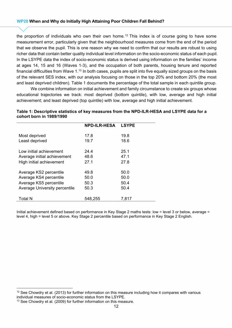
We combine information on initial achievement and family circumstance to create six groups whose educational trajectories we track: most deprived (bottom quintile), with low, average and high initial achievement; and least deprived (top quintile) with low, average and high initial achievement.

Table 1: Descriptive statistics of key measures from the NPD-ILR-HESA and LSYPE data for a cohort born in 1989/1990

NPD-ILR-HESA LSYPE Most deprived 17.8 19.8 Least deprived 19.7 18.6 Low initial achievement 24.4 25.1 Average initial achievement 48.6 47.1 High initial achievement 27.1 27.8 Average KS2 percentile 49.8 50.0 Average KS4 percentile 50.0 50.0 Average KS5 percentile 50.3 50.4 Average University percentile 50.3 50.4 Total N 548,255 7,817

Initial achievement defined based on performance in Key Stage 2 maths tests: low = level 3 or below, average = level 4, high = level 5 or above. Key Stage 2 percentile based on performance in Key Stage 2 English.

12 See Chowdry et al. (2013) for further information on this measure including how it compares with various individual measures of socio-economic status from the LSYPE. 13 See Chowdry et al. (2009) for further information on this measure.

13


4. Empirical approach

When assessing the educational trajectories of children by their initial attainment and family background, it is important to recognise the potential regression to the mean (RTM) issues described in Jerrim and Vignoles (2013). Any child defined as having ‘high’ or ‘low’ achievement on any given day may have over- or under-performed relative to their ‘true’ attainment, meaning that the next time they are tested they will look more like the average individual. When viewed over time as an educational trajectory, this statistical artefact would drive those from ‘high’ and ‘low’ initial achievement groups towards the mean value, creating an artificial convergence in educational trajectories across the two points in childhood. Jerrim and Vignoles (2013) emphasise that any measurement error in the test that is used to define initial attainment will be more prominent in the tails of the distribution, where the sample sizes are smaller, and hence this is the case for the ‘low’ and ‘high’ initial achievement groupings. Finding that high attaining poor children fall behind their lower achieving but better-off peers may therefore arise, at least in part, as a result of regression to the mean. If we do not try to account for this phenomenon, then our conclusions regarding the trajectories of children from different socio-economic backgrounds – and, in particular, whether and at what point high attaining poor children appear to fall behind relative to their lower achieving more advantaged peers – may be misleading.

The problem of RTM is exacerbated by defining initial attainment groupings based on measures that are then also used to plot educational trajectories over time. We use standard methods to account for the regression to the mean problem described above, namely a method initially proposed by Ederer (1972) (see also Davis (1974) and Marsh and Hau (2002)) and implemented by Jerrim and Vignoles (2013). This involves having two test scores taken at the same time point (t1) and using one of these tests to determine which group can be classified as “high achieving” and which “low achieving”, and using the other test as the baseline observation from which changes in achievement are measured. Defining initial achievement using a different test, measured at the same age, will go some way to reducing any effect of RTM by reducing the correlation (and hence measurement error) between the initial grouping and the first observed attainment measure. Specifically, we use performance in Key Stage 2 maths to define whether a child has high, average or low achievement at baseline, and Key Stage 2 English scores as the basis from which change in achievement is tracked.14

For the later of our two cohorts, we also adopt a second, very similar approach, in which we use a test score measured at an earlier time point (t0) to determine whether a child is high, average or low achieving, and then start measuring trajectories of attainment from t1. Any measurement error in the initial test should not be correlated with measurement error in a test taken at a different time period (based on the classical measurement error assumption of no serial correlation). This method should therefore, in principle, be even more robust to the presence of RTM than the first. In this case, we use performance in maths at Key Stage 1 (age 7) to define whether a child has high average or low achievement at baseline, and Key Stage 2 English as the starting point for tracking their education trajectory.15

In both data sources, information from the NPD is used to rank individuals within the distribution of overall attainment from Key Stage 2 through to Key Stage 5. Percentile rank at Key Stage 2 is based on a pupil’s fine grade score in English16 and percentile rank at Key Stage 4 is based on their average GCSE

14 We also check that our results hold by defining initial achievement based on English and using Maths as the starting point from which change is measured instead; our results are robust to these choices. 15 Again, our results are robust to using Key Stage 1 reading to define initial achievement and Key Stage 2 maths as the starting point from which trajectories are tracked. 16 We use mathematics when English is used to define initial attainment.

14


point score across all subjects17. For those who participate at Key Stage 5, percentile rank is defined based on their average A level point score18. In each case, attainment is standardised within sample. We do not observe any measures of attainment at university for those who attend, but we do observe the institution that they attend. This information comes from HESA data in the NPD-ILR-HESA dataset19 and from direct survey responses in the LSYPE.20 We define an individual’s percentile ranking based on their institution’s average score from the 2001 Research Assessment Exercises.21 Clearly one might have used alternative rankings of universities to judge the pupil’s university attainment. Indeed one might also use ranking of degree subjects and institutions. For our purposes however, we argue that RAE ranking is a reasonable proxy measure for institutional quality, however, as it has been shown to be correlated with various indicators of quality, such as class size and contact hours.

When defining percentile rank at Key Stage 5 and university, we encounter issues in assigning a ranking for those who do not participate. To overcome this issue, we take the following approach: for those who do not participate at Key Stage 5, we assign them a ranking based on their predicted probability of participation from a probit model of participation and prior attainment at Key Stage 4.22 For those who do not participate at university, we similarly assign a ranking based on their predicted probability of participation from a probit model based on their prior attainment at Key Stage 4 and 5. The underlying models are presented in Appendix Table A1 and the predicted percentile rankings by participation are reported for each of our six groups in Appendix Table A2. In both cases, individuals who do not participate are allocated a ranking below those who do participate. This assignment process allows us to distinguish between those who may have had the grades to stay on in education but chose not to do so and those who were not able to make the choice to stay on as their prior attainment was too low. Table 1 shows the mean percentiles across the two data sources (NPD-ILR-HESA and LSYPE) to be around 50.5, as expected.

To consider what might be driving our trends in educational trajectories we consider the conditional educational distribution of our sample of children after controlling for characteristics that are likely to drive differences in these trends. We begin by controlling for individual-level characteristics that are fixed over time including gender, ethnicity and month of birth. We do not anticipate that these are a major driver of the story.

Next we add in school-level fixed effects to condition on any differences between schools that might be driving these trends. It is well known that sorting into schools on the basis of socio-economic background is extensive (Allen and Vignoles, 2007; Allen, 2007) and that sorting is moderately high in England compared to other countries (Jenkins et al. 2008). Part of the mechanism through which such social segregation occurs is via the property market, with wealthier parents able to purchase houses nearer to certain sought after state-funded schools (Gibbons and Machin, 2003; Allen et al. 2010). A small percentage of pupils in England (around 7%) also attend private schools at age 16, with sorting occurring more explicitly on parents’ ability to pay in this case. In addition, in some areas, sorting into schools occurs

17 The results are very similar if we measure Key Stage 4 attainment based on the combined English and maths points score. 18 Or their individual Learner Record (ILR) score for those missing A level points in the NPD-ILR-HESA data. Unfortunately this data is not available in the LSYPE. 19 182765 respondents in the raw data reported an identifiable institution in the 1989/90 linked NPD-ILR-HESA data. 2327 report an unidentifiable institution. 33% of our final sample attended an identifiable university. 20 3291 respondents in the raw data reported an identifiable institution in the LSYPE. 194 report an unidentifiable institution. 27% of our final sample attended an identifiable university. 21 Note in the LSYPE the information on the institution attended is available only from the secure access data. We thank the University of Essex for the use of the Secure Data Server to allow us to analyse this variable. 22 We have finer grade measures of prior attainment available in the NPD-ILR-HESA data including subject choice so we supplement our LSYPE analysis to include KS2 attainment.

15


on the basis of ability rather than socio-economic background (although the two are, of course, highly correlated): while the percentage of pupils in England attending academically selective schools is small (less than 5%), it is much higher in areas which operate a grammar school system, such as Buckinghamshire or Kent.

We explore the extent to which sorting into schools can help to explain different academic trajectories by accounting for secondary school fixed effects. This enables us to control for any differences that arise because pupils from different backgrounds with differing primary school attainment go on to attend different secondary schools, and does not require us to assume that the (unobserved) school characteristics are orthogonal to the variables included in the model, as would be required with a random effects or multi-level model (Clarke et al. 2010). Whilst the fixed effects model comes at the cost of a loss in efficiency compared to the random effects model, in this instance we know there is substantial sorting into schools by socio-economic background and hence the fixed effects model is the more conservative choice. 23

Finally, we use the wealth of information available in the LSYPE data to define a set of scales that capture the educational values of both the child and the parents, along with their aspirations for post-16 outcomes and their expectations regarding higher education participation. Previous work by Goodman and Gregg (2010) has suggested that parental and child aspirations and beliefs – including parental aspirations regarding whether or not they want their child to attend higher education, and the extent to which parents or children believed that their own actions can affect their lives, i.e. the extent of their locus of control – can explain some of the socio-economic gap in pupil achievement and educational progress. For instance, nearly four out of five of the richest mothers in the Millennium Cohort Study hoped their child would go to university, compared to just over a third of the poorest mothers. These factors are certainly correlated with differences in attainment, and may help to explain the socio-economic gap in attainment. For example, they find that the difference in aspirations between parents from different socio-economic groups accounts for 6% of the attainment gap between the richest and poorest children at the end of primary school, controlling for prior attainment. (Equivalently, that they explain 6% of the difference in progress between Key Stage 1 and Key Stage 2.)

Both we and the authors of the above study recognise that attitudes, aspirations and expectations measured in the mid teen years are of course potentially endogenous and the consequence of relatively high or low achievement rather than the cause of it. Despite using the earliest measures available in the LSYPE (age 14), they may reflect the child’s educational trajectory rather than explain it. Hence we view this part of the analysis as indicative and descriptive only. Nonetheless it is of interest to explore how the declining trajectories of initially high attaining poor students change when allowing for differences in their or their family’s educational values, aspirations and expectations. The method we use to account for differences in demographic characteristics, school effects and aspirations/expectations is to regress the attainment measure at age 16 on our range of pupil characteristics and school fixed effects, and then to consider the average positions of those from our six prior attainment/SES groups after controlling for these differences (in the residual distribution of attainment).

23 Note that we are unable to measure school processes, for example steaming, which may be an important part of the story.

16


5. Results

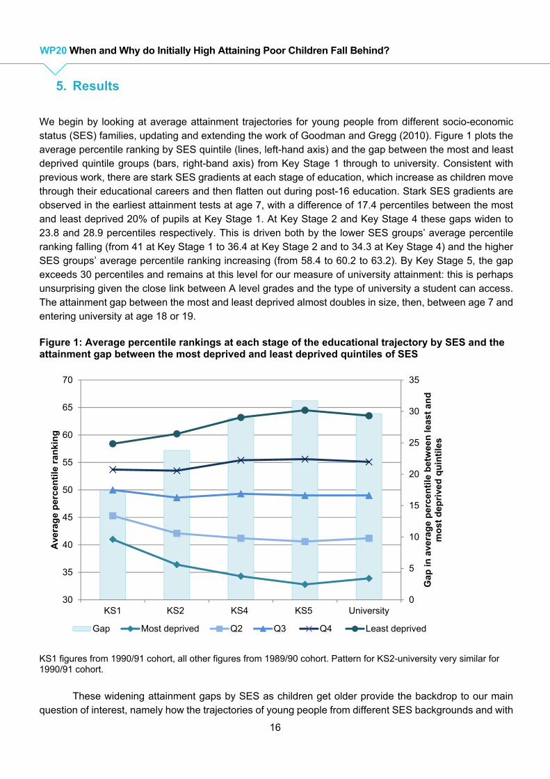
We begin by looking at average attainment trajectories for young people from different socio-economic status (SES) families, updating and extending the work of Goodman and Gregg (2010). Figure 1 plots the average percentile ranking by SES quintile (lines, left-hand axis) and the gap between the most and least deprived quintile groups (bars, right-band axis) from Key Stage 1 through to university. Consistent with previous work, there are stark SES gradients at each stage of education, which increase as children move through their educational careers and then flatten out during post-16 education. Stark SES gradients are observed in the earliest attainment tests at age 7, with a difference of 17.4 percentiles between the most and least deprived 20% of pupils at Key Stage 1. At Key Stage 2 and Key Stage 4 these gaps widen to 23.8 and 28.9 percentiles respectively. This is driven both by the lower SES groups’ average percentile ranking falling (from 41 at Key Stage 1 to 36.4 at Key Stage 2 and to 34.3 at Key Stage 4) and the higher SES groups’ average percentile ranking increasing (from 58.4 to 60.2 to 63.2). By Key Stage 5, the gap exceeds 30 percentiles and remains at this level for our measure of university attainment: this is perhaps unsurprising given the close link between A level grades and the type of university a student can access. The attainment gap between the most and least deprived almost doubles in size, then, between age 7 and entering university at age 18 or 19. Figure 1: Average percentile rankings at each stage of the educational trajectory by SES and the attainment gap between the most deprived and least deprived quintiles of SES

KS1 figures from 1990/91 cohort, all other figures from 1989/90 cohort. Pattern for KS2-university very similar for 1990/91 cohort.

These widening attainment gaps by SES as children get older provide the backdrop to our main

question of interest, namely how the trajectories of young people from different SES backgrounds and with

0

5

10

15

20

25

30

35

30

35

40

45

50

55

60

65

70

KS1 KS2 KS4 KS5 University

Gap

in a

vera

ge

per

cen

tile

bet

wee

n le

ast

and

m

ost

dep

rive

d q

uin

tile

s

Ave

rag

e p

erce

nti

le r

anki

ng

Gap Most deprived Q2 Q3 Q4 Least deprived

17


different initial achievement develop through school. We focus in particular on children from poor SES backgrounds who perform very well during primary school, exploring what happens as they move through the education system, and in particular whether and when they fall behind their lower-achieving but better-off peers.

Figure 2 plots the average percentiles of those from the most and least deprived families who were high, average and low achievers in their age 11 maths tests at Key Stage 2 for our main cohort (those born in 1989/90). It can be seen that lower-achieving affluent children catch up with higher-achieving deprived children between Key Stage 2 and Key Stage 4. Conversely, high-achieving children from the most deprived families fall behind lower-achieving students from the least deprived families by Key Stage 4. This pattern is consistent across the two data sources (see Appendix Figure A1 for LSYPE trajectories). Note that while there is some further convergence between these groups at Key Stage 5, most of the movement occurs between Key Stage 2 and Key Stage 4. This suggests that the period of compulsory secondary schooling is a crucial time in which children from deprived families are in danger of falling behind their similarly achieving affluent peers. We look into what might be driving these differences later in this section. Figure 2: Trajectories from Key Stage 2 to university for a NPD-ILR-HESA cohort born in 1989/1990 by initial achievement (Key Stage 2 maths) for the most deprived and least deprived quintiles of SES

Group size N= 37096, 46601, 14004, 14951, 50783, 41986

While we use different measures to split children into high, average and low initial achievement

groups and as the starting point for our education trajectories, there may still be some concern that our main finding of convergence between Key Stage 2 and Key Stage 4 is driven by RTM if scores in these tests is correlated for reasons other than ‘true’ performance - for example, if the pupil took both tests on a particularly ‘good’ or particularly ‘bad’ day and therefore performed unusually well or unusually badly on both measures.

Figures 3 and 4 investigate the role of regression to the mean in driving our findings by replicating the results in the NPD-ILR-HESA data for a cohort born one year later in 1990/91. The advantage of using this later cohort is that they were the first to sit Key Stage 1 tests and we can therefore contrast the educational trajectories based on initial achievement at Key Stage 1 compared to Key Stage 2 for this

0

20

40

60

80

100

KS2 KS4 KS5 University

Per

cen

tile

ran

kin

g

Most deprived High initial achievement

Most deprived Average initial achievement

Most deprived Low initial achievement

Least deprived High initial achievement

Least deprived Average initial achievement

Least deprived Low initial achievement

High

Low

Average

18


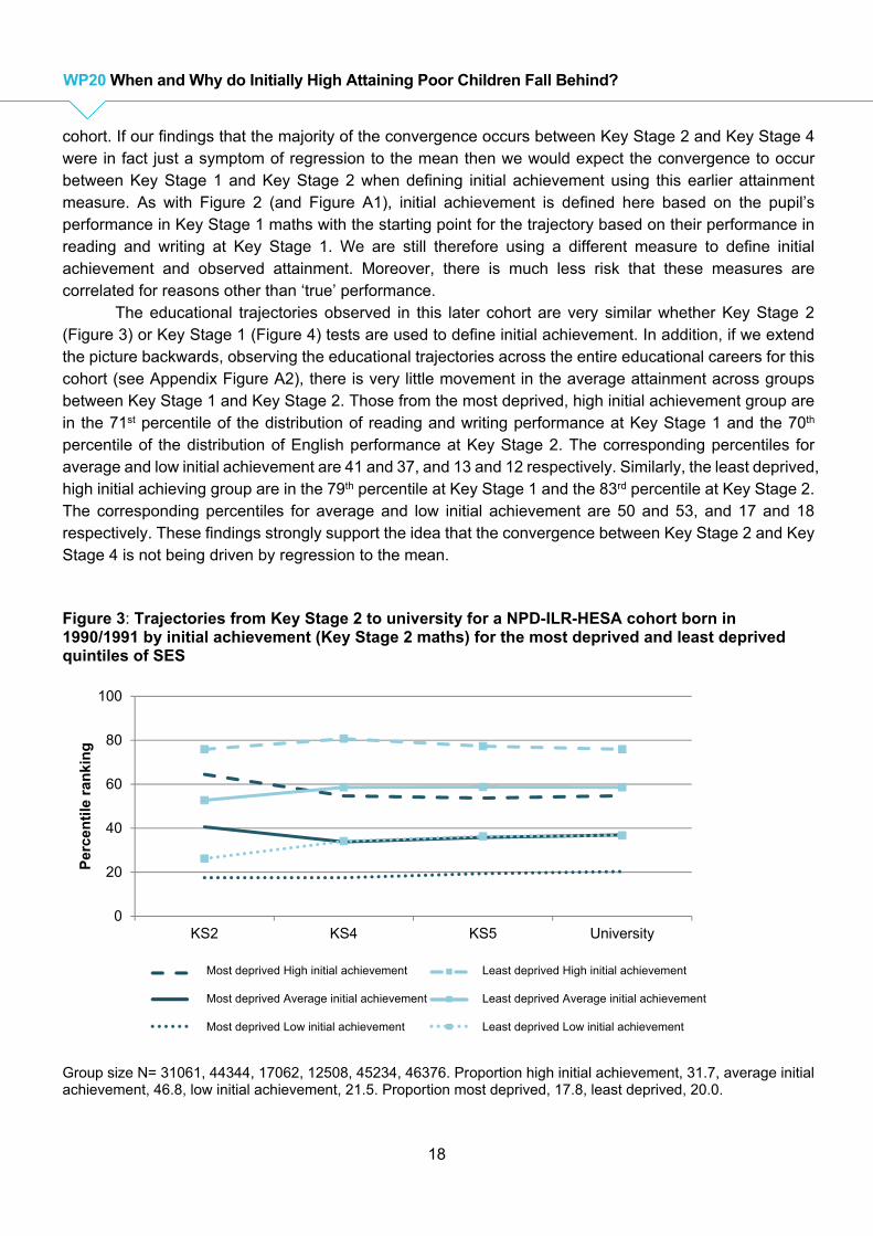
cohort. If our findings that the majority of the convergence occurs between Key Stage 2 and Key Stage 4 were in fact just a symptom of regression to the mean then we would expect the convergence to occur between Key Stage 1 and Key Stage 2 when defining initial achievement using this earlier attainment measure. As with Figure 2 (and Figure A1), initial achievement is defined here based on the pupil’s performance in Key Stage 1 maths with the starting point for the trajectory based on their performance in reading and writing at Key Stage 1. We are still therefore using a different measure to define initial achievement and observed attainment. Moreover, there is much less risk that these measures are correlated for reasons other than ‘true’ performance.

The educational trajectories observed in this later cohort are very similar whether Key Stage 2 (Figure 3) or Key Stage 1 (Figure 4) tests are used to define initial achievement. In addition, if we extend the picture backwards, observing the educational trajectories across the entire educational careers for this cohort (see Appendix Figure A2), there is very little movement in the average attainment across groups between Key Stage 1 and Key Stage 2. Those from the most deprived, high initial achievement group are in the 71st percentile of the distribution of reading and writing performance at Key Stage 1 and the 70th percentile of the distribution of English performance at Key Stage 2. The corresponding percentiles for average and low initial achievement are 41 and 37, and 13 and 12 respectively. Similarly, the least deprived, high initial achieving group are in the 79th percentile at Key Stage 1 and the 83rd percentile at Key Stage 2. The corresponding percentiles for average and low initial achievement are 50 and 53, and 17 and 18 respectively. These findings strongly support the idea that the convergence between Key Stage 2 and Key Stage 4 is not being driven by regression to the mean.

Figure 3: Trajectories from Key Stage 2 to university for a NPD-ILR-HESA cohort born in 1990/1991 by initial achievement (Key Stage 2 maths) for the most deprived and least deprived quintiles of SES

Group size N= 31061, 44344, 17062, 12508, 45234, 46376. Proportion high initial achievement, 31.7, average initial achievement, 46.8, low initial achievement, 21.5. Proportion most deprived, 17.8, least deprived, 20.0.

0

20

40

60

80

100


Per

cen

tile

ran

kin

g







19


Figure 4: Trajectories from Key Stage 2 to university for a NPD-ILR-HESA cohort born in 1990/1991 by initial achievement (Key Stage 1 maths) for the most deprived and least deprived quintiles of SES

Group size N= 13865, 65907, 12681, 4478, 64662, 34929. Proportion high initial achievement, 24.9, average initial achievement, 67.4, low initial achievement, 8.7. Proportion most deprived, 17.8, least deprived, 20.0. Key Stage 1 percentiles: 12.9, 41.2, 70.5, 17.0, 50.0, 79.2.

As additional robustness checks, Appendix Figures A3 and A4 replicate the trends observed in Figure 2 and Figure A2 using an alternative definition of initial achievement based on pupils’ performance in age 11 English tests at Key Stage 2 and plots the trajectory using Key Stage 2 maths scores as a starting point. While the trends are slightly different for this definition of initial achievement, it is still the case that the majority of the convergence between high achieving deprived pupils and average achieving affluent pupils, and low achieving affluent pupils and average achieving deprived pupils, again occurs between Key Stage 2 and Key Stage 4.

Drivers of educational trajectories

Given our finding that compulsory secondary schooling is a period in which high achieving poorer children are in danger of falling behind their more affluent peers, we move on to assess the potential role of key background characteristics, schools and education values, expectations and aspirations in explaining the change in performance between Key Stage 2 and Key Stage 4. Table 2 describes differences in key background characteristics by initial achievement and SES grouping. It shows that girls are less likely to be found in the high achieving groups for both high and low SES families, highlighting their relatively weaker performance in KS2 maths compared to boys, but the pattern across groups is fairly consistent and the results are similar when we use KS2 English as an alternative measure.

0

20

40

60

80

100


Per

cen

tile

ran

kin

g








Table 2: Descriptive statistics of key measures of demographics and school characteristics by SES status and initial achievement

All High SES Low SES High initial

achievement Average initial achievement

Low initial achievement

High initial achievement

Average initial achievement


Female 50.1 46.7 51.4 51.4 44.4 51.1 54.1 Ethnicity White 86.1 91.4 91.9 90.5 78.8 80.2 80.3 Mixed 2.1 2.7 2.4 2.3 2.0 1.9 1.8 Indian 1.1 0.2 0.3 0.4 2.5 2.5 2.3 Pakistani 1.3 0.2 0.4 0.7 1.9 2.4 2.6 Bangladeshi 0.4 0.1 0.2 0.2 0.7 0.7 0.8 Black Caribbean 2.3 1.7 1.5 1.7 1.7 1.3 1.1 Black African 2.2 0.4 0.6 1.1 3.6 3.7 4.7 Chinese 0.9 0.1 0.1 2.8 3.2 2.5 2.4 Other White 0.3 0.5 0.2 1.3 0.7 0.3 0.2 Other Black 0.5 0.4 0.4 3.7 0.6 0.5 0.3 Other Asian 2.1 1.8 1.6 1.7 2.9 3.0 2.7 Other 0.7 0.4 0.4 5.0 1.4 1.0 0.9 Month of birth September 8.2 9.7 7.4 5.8 10.8 8.6 6.8 October 8.2 9.5 7.5 6.2 11.0 8.4 7.1 November 7.9 8.9 7.3 6.2 9.6 8.5 7.1 December 8.1 8.5 7.6 6.5 9.7 8.5 7.7 January 8.1 8.2 7.9 7.3 8.7 8.5 8.1 February 7.6 7.5 7.8 7.1 8.0 7.8 7.7 March 8.5 8.5 8.7 8.5 7.8 8.6 8.3 April 8.2 8.3 8.5 8.5 7.3 7.9 8.4 May 8.8 8.2 9.0 10.2 7.3 8.4 9.3 June 8.7 7.9 9.5 10.9 6.8 8.2 9.2 July 8.9 7.7 9.5 11.3 6.7 8.6 10.0 August 8.7 7.1 9.3 11.6 6.3 8.0 10.2 School performance School CVA KS2-KS4 1000.3 1002.4 1001.84 1001.71 999.32 999.45 999.87 School 5 A*-C at KS4 60.4 73.1 66.5 62.6 53.8 50.1 47.7



There are some notable differences across SES groups in terms of ethnicity with high SES children more likely to be white and low SES children more likely to be Indian or Black African in particular, but there is little variation by ethnicity in terms of the likelihood of being in a particular initial achievement group within a SES group. The picture for month of birth is reversed with little difference across SES groups since birth months are randomly distributed but fairly stark differences, as is expected, across initial achievement grouping with those born earlier in the academic year more likely to be defined as high achieving and those born later in the academic year comprising a greater proportion of the low achieving group.

The final two lines of Table 2 illustrate the average performance of the schools attended by these different groups. We measure school performance in two ways: first using the Department for Education’s contextualised value-added (CVA) measure; second, in terms of overall Key Stage 4 performance. While the CVA measure accounts for the differential composition of a school’s intake, the latter partly reflects the different intakes of schools as well as their quality. There are obvious differences across both SES and initial achievement groups in these school performance measures. High achieving affluent children, on average, attend the best performing schools and low achieving deprived children, on average, attend the worst performing schools. These patterns are more clear cut in terms of the overall performance measure than in terms of the CVA measure.

To consider the role of these differences in background characteristics and school choice in explaining the observed attainment distributions at Key Stage 4, we regress Key Stage 4 attainment on these measures and summarise the residuals for each of our six groups. We build our model in stages, first accounting individual-level characteristics (specifically gender, ethnicity and month of birth), before moving to a school fixed effects model in order to assess how much of the pattern remains once we compare children who attend the same schools (see Appendix Table A3 for full estimates from these models). We plot average percentile rankings for each of our six groups at Key Stage 2 and Key Stage 4, where our Key Stage 4 ranking is generated using the residuals from a model of educational attainment, after differences in demographic characteristics and school attended are accounted for.

Figure 5, panel A replicates the unconditional trajectory from Figure 1 while panel B plots the trajectory conditional on ethnicity, gender and month of birth. As can be seen, controlling for observed differences in these key individual-level characteristics does little to change the picture of educational trajectories over this crucial period. Panel C of Figure 5 illustrates the educational trajectories between Key Stage 2 and Key Stage 4 after controlling for differences in these individual-level characteristics and differences between schools (school fixed effects). This specification essentially removes any differences that will be driven by children sorting into different types of schools and school segregation, focusing on the remaining attainment distribution within similar schools.

Panel C indicates that, once differences between schools are controlled for, the extent of the convergence in attainment between initially high achieving poor children and initially lower achieving affluent is lessened significantly. This indicates that part of the reason for the observed convergence seen in the unconditional models seems to be because pupils from different backgrounds and with differing prior attainment go to different schools, i.e. because of school sorting and segregation. This suggests that selection into schools is based on initial achievement as well as family background, as was indeed indicated by Table 2. Note that these patterns of conditional trajectories are very similar for the LSYPE cohort (see Appendix Figure A5). In other words poorer children who are initially higher achieving attend lower performing schools than their wealthier counterparts and this explains some of the difference in educational trajectories between these two groups.

22


Figure 5: Trajectories from Key Stage 2 to Key Stage 4 for a cohort born in 1989/1990 by initial achievement (Key Stage 2 maths) for the most deprived and least deprived quintiles of SES, conditional on demographics, school fixed effects and values, aspirations and expectations.

More generally we observe a narrowing of the average differences in attainment between rich

initially high achieving pupils and poor initially low achieving pupils, indicating that schools may be focusing their resources on the lowest achieving pupils with these pupils showing greater catch-up with average achieving pupils. There is some suggestion this may come at a cost to the highest achieving pupils, particularly from high SES families, who are experiencing some degree of convergence with their average achieving peers within schools. Whilst these patterns cannot prove a causal link between school quality and pupil achievement, they are suggestive. These results are also clearly indicative of the strength of school sorting even within SES groups.

Finally, to explore the role of education values, expectations and aspirations in the pattern of convergence that we see between Key Stage 2 and Key Stage 4, we turn to the LSYPE data and add a range of measures of these characteristics to our specification. We acknowledge that these characteristics are potentially endogenous, given that they will be driven in part by initial achievement, and we emphasise

Panel C: Conditional on demographics and school fixed effects (NPD)

Group size N= 37096, 46601, 14004, 14951, 50783, 41986

0

20

40

60

80

100

KS2 KS4

Per

cen

tile

ran

kin

g

Panel D: Conditional on demographics, school fixed effects and values, aspirations and expectations (LSYPE)

Group size N= 629, 725, 241, 114, 603, 742

0

20

40

60

80

100

KS2 KS4

Per

cen

tile

ran

kin

g

Panel A: Unconditional (NPD)

Group size N= 37096, 46601, 14004, 14951, 50783, 41986

0

20

40

60

80

100

KS2 KS4

Per

cen

tile

ran

kin

g







Panel B: Conditional on demographics (NPD)

Group size N= 37096, 46601, 14004, 14951, 50783, 41986

KS2 KS4

23


that we are not attempting to place a causal interpretation on our findings. Instead we are interested in comparing the conditional trajectories across groups after controlling for observed differences in these values, aspirations and expectations, regardless of how these are formed.

Table 3 summarises the average level of the scales of education values, aspirations and expectations at age 14 by SES and initial achievement group. There are large differences in the pupil level scales by both SES grouping and initial achievement grouping, with those from higher SES families reporting higher scores for ability beliefs, and intrinsic and extrinsic value of schooling scales. Those from the higher initial achievement groups report higher values in these scales than those from lower initial achievement groups. The pattern is similar across aspirations and expectations although there are a notable number of high initial achieving low SES pupils that report lower aspirations and expectations. The parental aspirations and expectations measures follow a similar pattern to those observed with the pupil reported characteristics. However, the parents of high initial achieving deprived children appear to have higher aspirations and expectations than their more affluent but lower attaining counterparts (e.g. those in the average initial achieving affluent group), despite the aspirations and expectations of the pupils in these groups being very similar. Interestingly, the education value scale varies quite dramatically by group with those from high SES families typically having a lower value of education, particularly if their child has low or average initial achievement. Those from lower SES families highly value education across the board although those with higher initial achieving pupils value it more than those with lower initial achieving children. It is unclear why this might be and it appears to be somewhat counterintuitive. It may imply however, that for poor families it is more apparent that education is critically important for the success of their children, whilst in richer families the success of less able children in particular may not be so strongly linked to their educational success.

The final column of Appendix Table A2 suggests that the majority of these characteristics are significant predictors of attainment at Key Stage 4, corrobating the findings of Chowdry et al (2009): pupils with a greater belief in their ability, and a higher intrinsic and extrinsic value of school do indeed have a higher percentile ranking at Key Stage 4. Those who express a desire to do something other than continue on in full time education after age 16 perform worse at Key Stage 4, while those who believe they are not likely to apply or get in to university perform worse than those who are likely to apply and get in. The patterns are very similar in terms of parental aspirations and expectations and of a similar magnitude.

The final panel of Figure 5 plots the trajectories for those children with similar demographics, school characteristics and educational values, aspirations and expectations. Once we control for these measures, compared to panel C, there is generally much more convergence in the educational trajectories between Key Stage 2 and Key Stage 4 for all groups. In other words, some of the differences in children’s trajectories, regardless of initial achievement or SES, are explained by the educational values, aspirations and expectations they hold. This suggests that when we take out observable differences in pupil aspirations and attitudes, achievement gaps are less pronounced, as we might expect given that some of these aspirations and attitudes are themselves driven by pupils’ achievements. But interestingly, aspirations and attitudes do also help to explain part of the difference between SES within initial attainment groups, especially amongst average and higher achieving pupils. This suggests that socio-economic differences in education values, aspirations and expectations are not simply driven by differences in prior attainment, but rather that, even comparing those with similar levels of high or low initial attainment and expectations and aspirations, pupils from richer families are more able to turn these observed characteristics into attainment gains at age 16.


Table 3: Descriptive statistics of key measures of pupil and parent reported ability belief and education value scales, aspirations and expectations at age 14 from the LSYPE data for a cohort born in 1989/1990, by SES status and initial achievement

All High SES Low SES

Child reported High initial achievement






Ability belief scale -0.003 0.365 -0.020 -0.343 0.290 -0.064 -0.212 Intrinsic value scale -0.007 0.138 -0.003 -0.030 0.100 -0.074 -0.161 Extrinsic value scale -0.009 0.171 0.081 -0.086 0.096 -0.025 -0.272 Post-16 aspirations Stay on in FTE at 16 85.2 98.1 92.5 74.7 92.8 82.5 69.5 Enter FT work at 16 4.7 0.4 1.2 7.2 1.7 5.6 15.7 Learn a trade 7.0 0.5 2.7 14.9 4.6 8.6 10.3 Other 2.9 1.1 3.6 3.2 0.9 3.3 4.1 Higher education expectations Likely to apply 69.3 94.3 82.8 56.3 85.3 60.9 51.2 Not very likely to apply 18.3 4.2 12.3 25.7 8.8 24.0 19.2 Not at all likely to apply 12.4 1.5 4.9 18.1 5.9 15.1 29.5 Likely to get in 82.8 98.6 89.5 63.9 94.5 76.0 68.5 Not very likely to get in 15.6 1.4 10.5 36.1 5.3 20.8 29.3 Not at all likely to get in 1.6 0.0 0.1 0.0 0.2 3.2 2.2

Parent reported

Education value scale -0.002 0.089 -0.036 -0.206 0.186 0.088 0.075 Post-16 aspirations Stay on in FTE at 16 81.2 97.0 91.7 70.7 90.6 73.0 72.0 Enter FT work at 16 1.7 0.0 0.5 0.0 0.8 4.0 5.7 Learn a trade 15.9 1.9 6.7 26.1 7.2 21.6 22.1 Other 1.2 1.1 1.0 3.2 1.4 1.4 0.2 Higher education expectations Likely to attend 63.4 95.3 77.1 41.5 87.6 56.5 37.5 Not very or not at all likely to attend

36.6 4.7 22.9 58.5 12.4 43.5 62.5


While conditioning on these factors suggests what might be contributing to the observed patterns in the trajectories by grouping, this method has obvious limitations in that there may be other unobserved factors driving these findings including parental resources within SES groupings. In addition, care needs to be exercised when interpreting the findings relating to expectations and aspirations as one cannot conclude that altering pupils’ attitudes and aspirations would necessarily produce this convergence in attainment since differences in attitudes and aspirations may be instead the product of differences in attainment. This evidence is therefore indicative of potential areas for further consideration rather than conclusive proof of the role of schools or aspirations and expectations.

26


6. Conclusions

This paper has investigated when and why initially high attaining children from deprived backgrounds fall behind their lower achieving but better-off peers. We find clear evidence of a convergence of cognitive achievement during secondary school between affluent children of lower initial attainment and poorer children of higher initial attainment. Even if a poor child starts out with high attainment at age 11, by the time they reach GCSE they have fallen behind relative to their more affluent high achieving peers. By contrast, a richer child of lower attainment at age 11 manages to catch up somewhat by age 16 and converge, in terms of their achievement, towards the trajectory of poor but more able children. This finding is not driven by the problem of regression to the mean.

Our analysis indicates that some of the convergence that we observe is attributable to the fact that poor children attend different schools from their richer counterparts and these schools are lower performing across a number of dimensions. While we cannot prove that attending different quality schools is the cause of the patterns we observe, since there is substantial selective sorting into schools, the evidence does suggest that government policies should look to ensure that high achieving poor children have access to good quality secondary schools.

Our modelling has also suggested that students on these different trajectories have different educational values, aspirations and expectations. Once we control for these factors in our models the picture changes substantially and the trajectories of low/high SES and low/high initial achievement groups all start to converge. Hence differences in aspirations and expectations appear to play an important role in explaining why it is that the achievement of poor but able students declines relative to their more affluent counterparts. Again, however, our analysis is not necessarily causal and such differences in attitudes and aspirations may be the consequence of these pupils attending different schools and having different levels of attainment, rather than the cause. We therefore urge further investigation into this area rather than suggesting that this is conclusive proof of the role of aspirations and expectations in driving the attainment trajectories of young people from different backgrounds.

A lot of policy attention has been focused on trying to improve the achievement of poor children, with incentives provided to schools to focus more on these children (e.g. via the Pupil Premium). However, there has been less focus on high attaining children specifically. At a minimum, researchers and practitioners need to focus their efforts on better understanding why it is that high attaining poor children struggle to translate their early educational success into continued achievement in secondary school. Given the debate about whether the Pupil Premium might be more targeted, perhaps on under achieving poor children, it is timely to consider the objective of this policy and whether it should be more focused on helping poor children who are initially high achieving to achieve their potential.

Our results also support the increasing focus of outreach efforts by universities towards longer-term interventions earlier in the school system. In particular, our results suggest that universities may wish to pay particular attention to trying to maintain the attainment, attitudes and aspirations of high achieving children from disadvantaged backgrounds through secondary school. They may also wish to consider earlier measures of attainment when looking to attract pupils from deprived backgrounds with the most potential.

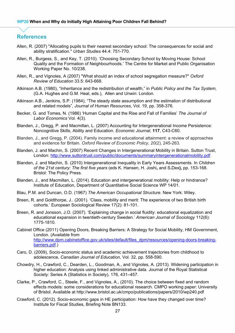
27


References

Allen, R. (2007) "Allocating pupils to their nearest secondary school: The consequences for social and ability stratification." Urban Studies 44.4: 751-770.

Allen, R., Burgess, S., and Key, T. (2010). ‘Choosing Secondary School by Moving House: School Quality and the Formation of Neighbourhoods.’ The Centre for Market and Public Organisation Working Paper No. 10/238.

Allen, R., and Vignoles, A (2007) "What should an index of school segregation measure?" Oxford Review of Education 33.5: 643-668.

Atkinson A.B. (1980), “Inheritance and the redistribution of wealth,” in Public Policy and the Tax System, (G.A. Hughes and G.M. Heal, eds.), Allen and Unwin: London.

Atkinson A.B., Jenkins, S.P. (1984), “The steady state assumption and the estimation of distributional and related models”, Journal of Human Resources, Vol. 19, pp. 358-376.

Becker, G. and Tomes, N. (1986) ‘Human Capital and the Rise and Fall of Families’ The Journal of Labor Economics Vol. 4(3).

Blanden, J., Gregg, P. and Macmillan, L. (2007) Accounting for Intergenerational Income Persistence: Noncognitive Skills, Ability and Education. Economic Journal, 117, C43-C60.

Blanden, J., and Gregg, P. (2004). Family income and educational attainment: a review of approaches and evidence for Britain. Oxford Review of Economic Policy, 20(2), 245-263.

Blanden, J. and Machin, S. (2007) Recent Changes in Intergenerational Mobility in Britain. Sutton Trust, London: http://www.suttontrust.com/public/documents/summaryintergenerationalmobility.pdf.

Blanden, J. and Machin, S. (2010) Intergenerational Inequality in Early Years Assessments. In Children of the 21st century: The first five years (eds K. Hansen, H. Joshi, and S.Dex), pp. 153-168. Bristol: The Policy Press.

Blanden, J., and Macmillan, L. (2014). Education and intergenerational mobility: Help or hindrance? Institute of Education, Department of Quantitative Social Science WP 14/01.

Blau, P.M. and Duncan, O.D. (1967) The American Occupational Structure. New York: Wiley.

Breen, R. and Goldthorpe, J.. (2001). ‘Class, mobility and merit: The experience of two British birth cohorts.’ European Sociological Review 17(2): 81-101.

Breen, R. and Jonsson, J.O. (2007). ‘Explaining change in social fluidity: educational equalization and educational expansion in twentieth-century Sweden.’ American Journal of Sociology 112(6): 1775-1810.

Cabinet Office (2011) Opening Doors, Breaking Barriers: A Strategy for Social Mobility, HM Government, London. (Available from http://www.dpm.cabinetoffice.gov.uk/sites/default/files_dpm/resources/opening-doors-breaking-barriers.pdf.)

Caro, D. (2009), Socio-economic status and academic achievement trajectories from childhood to adolescence, Canadian Journal of Education, Vol. 32, pp. 558-590.

Chowdry, H., Crawford, C., Dearden, L., Goodman, A., and Vignoles, A. (2013). Widening participation in higher education: Analysis using linked administrative data. Journal of the Royal Statistical Society: Series A (Statistics in Society), 176, 431–457.

Clarke, P., Crawford, C., Steele, F., and Vignoles, A., (2010). The choice between fixed and random effects models: some considerations for educational research. CMPO working paper: University of Bristol. Available at http://www.bristol.ac.uk/cmpo/publications/papers/2010/wp240.pdf

Crawford, C. (2012). Socio-economic gaps in HE participation: How have they changed over time? Institute for Fiscal Studies, Briefing Note BN133.

28


Crawford, C. (2014). The Link between Secondary School Characteristics and University Participation and Outcomes. Report to the Department for Education.

Cunha, F. Heckman, J. Lochner, L and Masterov, D. (2006) Interpreting the Evidence on Life Cycle Skill Formation. In Handbook of the Economics of Education (eds E. Hanushek and F. Welch), pp. 697-812. Amsterdam: Holland North.

Davis, C. (1976) The Effect of Regression to the Mean in Epidemiologic and Clinical Studies, American Journal of Epidemiology, 104, 493-498.

Duncan, G. and Magnuson, K. (2011) The Nature and Impact of Early Achievement Skills, Attention Skills and Behavior Problems. In Whither Opportunity? Rising Inequality, Schools, and Children’s Life Chances (eds G. Duncan and R. Murnane), pp. 47-69. New York: Russell Sage Foundation. Ederer, F. (1972) Serum Cholesterol: Effects of Diet and Regression Toward the Mean, Journal of Chronic Disorders, 25, 277-289.

Ederer, F. (1972) Serum Cholesterol: Effects of Diet and Regression Toward the Mean, Journal of Chronic Disorders, 25, 277-289.

Ermisch, J., Jantti, M., and Smeeding, T.M., (eds.) (2012) From parents to children: The intergenerational transmission of advantage. Russell Sage Foundation.

Feinstein, L. (2003) Inequality in the Early Cognitive Development of British Children in the 1970 Cohort, Economica, 70, 73-97.

Feinstein, L. (2004) Mobility in Pupils’ Cognitive Attainment During School Life, Oxford Review of Economic Policy, 20, 213-229.

Field, F. (2010) The Foundation Years: Preventing Poor Children Becoming Poor Adults, Independent Review on Poverty and Life Chances, Cabinet Office, London. (Available from http://webarchive.nationalarchives.gov.uk/20110120090128/http:/povertyreview.independent.gov.uk/media/20254/poverty-report.pdf.)

Galton, F. (1886) Regression Towards Mediocrity in Hereditary Stature, The Journal of the Anthropological Institute of Great Britain and Ireland, 15, 246–263.

Gibbons, S, and Machin, S., "Valuing English primary schools." Journal of Urban Economics 53.2 (2003): 197-219.

Goodman, A., & Gregg, P. (2010). Poorer Children’s Educational Attainment: How Important Are Attitudes and Behaviour? Report to the Joseph Rowntree Foundation.

Goodman, A., Gregg, P., & Washbrook, E. (2011). Children’s educational attainment and the aspirations, attitudes and behaviours of parents and children through childhood. Longitudinal and Life Course Studies, 2(1), 1-18.

Goodman A. Sibieta L. and Washbook E. (2009) Inequalities in Educational Outcomes Among Children Aged 3 to 16, Final report for the National Equality Panel, Institute for Fiscal Studies, London. (Available from http://sta.geo.useconnect.co.uk/pdf/Inequalities%20in%20education%20outcomes%20among%20children.pdf.)

Gorard, S, & Cheng, SC. (2011). ‘Pupil Clustering in English Secondary Schools: One Pattern or Several?’ International Journal of Research & Method in Education 34(3): 327-39.

Jenkins, S P., Micklewright, J. and Schnepf. S.V. (2008) "Social segregation in secondary schools: how does England compare with other countries?" Oxford Review of Education 34.1: 21-37.

Jerrim, J., & Vignoles, A. (2013). Social mobility, regression to the mean and the cognitive development of high ability children from disadvantaged homes. Journal of the Royal Statistical Society: Series A (Statistics in Society), 176: 887–906.

29


Marsh, H. and Hau, K. (2002) Multilevel Modelling of Longitudinal Growth and Change: Substantive Effects or Regression Toward the Mean Artefacts? Multivariate Behavioral Research, 37, 245-282.

Marmot M. (2010) Fair Society, Healthy Lives: The Marmott Review, Marmot Review, University College London, London. (Available from http://www.instituteofhealthequity.org/.)

Parsons, S. Schoon, I. Rush, R. and Law, J. (2011) Long-term Outcomes for Children with Early Language Problems: Beating the Odds, Children and Society, 25, 202 – 214.

Reardon, S. (2011) The Widening Academic Achievement Gap Between the Rich and the Poor: New Evidence and Possible Explanations. In Whither Opportunity? Rising Inequality, Schools, and Children’s Life Chances, (eds G. Duncan and R. Murnane), pp.91-116. New York: Russell Sage Foundation.

Schoon, I. (2006) Risk and Resilience: Adaptations in Changing Times, Cambridge: Cambridge University Press.

Strand, S. (2014a). Ethnicity, gender, social class and achievement gaps at age 16: Intersectionality and ‘Getting it’ for the white working class. Research Papers in Education, 29(2), 131-171.

Strand, S. (2014b). School effects and ethnic, gender and socio-economic gaps in educational achievement at age 11. Oxford Review of Education, 40(2), 223-245.

30


Appendix

Table A1: Marginal effects from probit models predicting participation at Key Stage 5 and university based on prior attainment at Key Stage 4 in the NPD-ILR-HESA cohort born in 1989/90

Participation at KS5 Participation at university

Key Stage 4 points score 0.013 (.000)*** 0.004 (.000)***

Key Stage 4 English A*-C 0.238 (.002)*** 0.061 (.002)***

Key Stage 4 maths A*-C 0.119 (.002)*** 0.043 (.002)***

Number of A*s in EBacc subs 0.113 (.002)*** 0.033 (.002)***

Number of As in EBacc subs 0.128 (.002)** 0.028 (.002)**

Number of Bs in EBacc subs 0.108 (.001)*** 0.021 (.001)***

Number of Cs in EBacc subs 0.068 (.001)*** 0.011 (.001)***

Participation at KS5 0.252 (.003)***

Key Stage 5 point score 0.002 (.000)***

Number of As in KS5 subs 0.092 (.002)***

Number of Bs in KS5 subs 0.092 (.002)***

Number of Cs in KS5 subs 0.072 (.001)**

Number of Ds in KS5 subs 0.038 (.001)***

Number of Es in KS5 subs -0.005 (.001)***

Pseudo R2 0.507 0.490

N 548,255 548,255

31


Table A2: Predicted percentile rankings at Key Stage 5and University by participation by initial achievement (Key Stage 2 maths) for the most deprived and least deprived quintiles of SES in the NPD-ILR-HESA cohort born in 1989/90

High SES Low SES High initial

achievement Average initial achievement





Participated at Key Stage 5 83.2 73.8 67.6 72.1 66.3 63.0 Did not participate at Key Stage 5 40.4 32.4 22.0 33.2 23.5 14.2 Participated at University 85.1 80.4 77.6 81.6 78.9 77.6 Did not participate at University 51.0 41.4 27.2 40.0 28.0 16.0

32


Table A3: Regressions coefficients predicting outcomes at Key Stage 4 based on demographics and school fixed effects in the NPD and LSYPE and child and parental values, aspirations and expectations at age 14 in the LSYPE

Cohort (model) NPD (1) NPD (2) LSYPE (1) LSYPE (2) LSYPE (3) Female 6.66 (0.76)*** 6.55 (0.73)*** 5.56 (0.78)*** 5.74 (0.71)*** 4.91 (0.57)*** White Baseline Baseline Baseline Baseline Baseline Mixed -0.59 (0.27)** -0.05 (0.25) 1.73 (2.33) -0.55 (1.85) -3.29 (1.51)** Indian 12.20 (0.26)*** 12.47 (0.27)*** 7.25 (1.34)*** 8.64 (1.75)*** -0.40 (1.56) Pakistani -1.80 (0.27)*** 4.22 (0.28)*** -7.20 (1.59)*** -0.47 (1.69) -8.39 (1.56)*** Bangladeshi 2.53 (0.41)*** 7.82 (0.44)*** -2.65 (2.03) -2.12 (2.51) -4.31 (2.10)** Black Caribbean -8.32(0.34)*** -4.10 (0.33)*** -7.84 (2.34)*** -6.28 (2.44)** -9.66 (2.13)*** Black African 0.72 (0.37)** 4.00 (0.36)*** 0.94 (2.73) 0.06 (2.44) -7.97 (2.26)*** Chinese 22.06 (0.70)*** 18.06 (0.63)*** Other White 5.49 (0.27)*** 3.26 (0.26)*** Other Black -7.47 (0.60)*** -3.73 (0.55)*** Other Asian 13.10 (0.55)*** 10.53 (0.51)*** Other 4.59 (0.48)*** 5.93 (0.46)*** 6.37 (3.22)** 5.65 (2.45)** -0.83 (2.20) Month of birth September Baseline Baseline Baseline Baseline Baseline October -0.33 (0.19)* -0.35 (0.17)** -2.62 (1.97) -3.94 (1.70)** -3.20 (1.29)** November -0.55 (0.19)*** -0.55 (0.17)*** -1.90 (1.97) -2.88 (1.66)* -1.64 (1.27) December -1.37 (0.19)*** -1.13 (0.17)*** 0.45 (1.92) -1.53 (1.68) -0.43 (1.29) January -1.68 (0.19)*** -1.48 (0.17)*** -4.15 (1.99)** -2.91 (1.99)* -2.07 (1.27) February -1.57 (0.19)*** -1.45 (0.17)*** -4.90 (1.93)** -5.48 (1.65)*** -3.22 (1.28)** March -1.75 (0.19)*** -1.77 (0.17)*** -1.84 (1.89) -2.83 (1.60)* -0.85 (1.25) April -1.97 (0.19)*** -1.81 (0.17)*** -7.78 (1.89)*** -6.09 (1.64)*** -2.86 (1.26)** May -2.48 (0.19)*** -2.22 (0.17)*** -5.17 (1.85)*** -5.38 (1.60)*** -2.89 (1.27)** June -2.83 (0.19)*** -2.65 (0.17)*** -3.09 (1.87)* -4.49 (1.57)*** -2.75 (1.23)** July -3.15 (0.18)*** -2.81 (0.16)*** -4.57 (1.85)** -5.86 (1.68)*** -2.56 (1.25)** August -3.76 (0.19)*** -3.29 (0.17)*** -7.10 (1.82)*** -6.94 (1.47)*** -2.66 (1.25)**

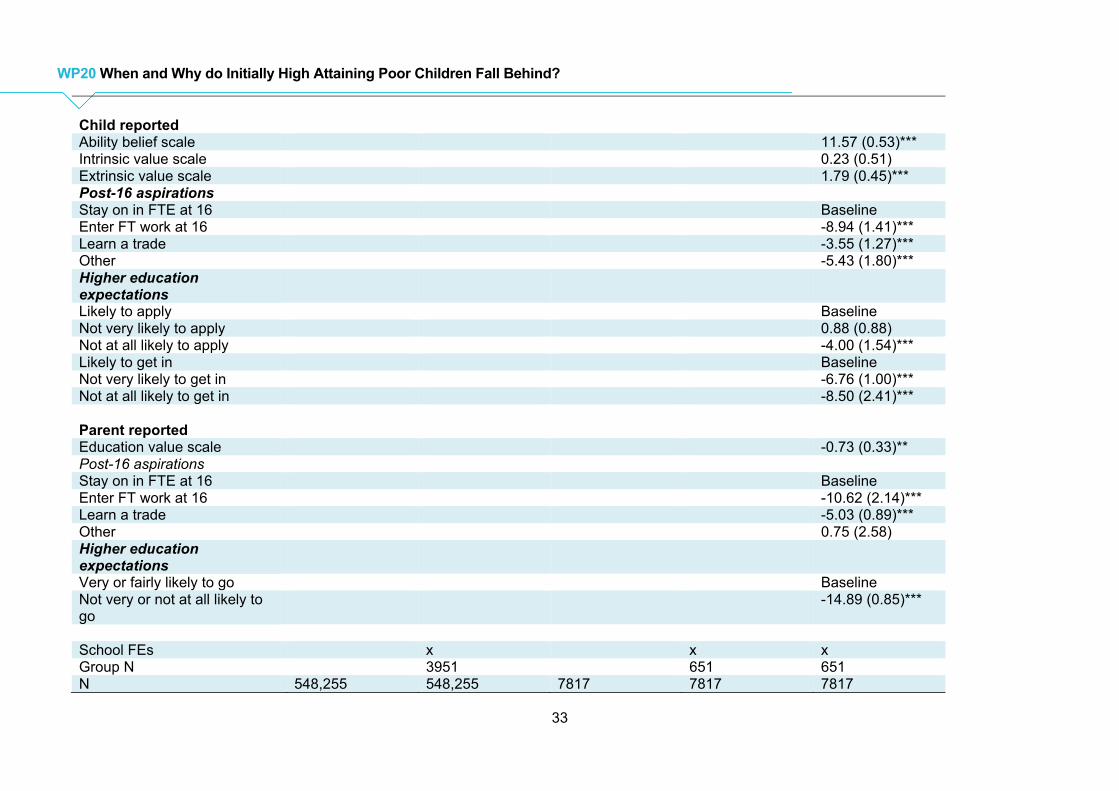
33


Child reported Ability belief scale 11.57 (0.53)*** Intrinsic value scale 0.23 (0.51) Extrinsic value scale 1.79 (0.45)*** Post-16 aspirations Stay on in FTE at 16 Baseline Enter FT work at 16 -8.94 (1.41)*** Learn a trade -3.55 (1.27)*** Other -5.43 (1.80)*** Higher education expectations

Likely to apply Baseline Not very likely to apply 0.88 (0.88) Not at all likely to apply -4.00 (1.54)*** Likely to get in Baseline Not very likely to get in -6.76 (1.00)*** Not at all likely to get in -8.50 (2.41)*** Parent reported Education value scale -0.73 (0.33)** Post-16 aspirations Stay on in FTE at 16 Baseline Enter FT work at 16 -10.62 (2.14)*** Learn a trade -5.03 (0.89)*** Other 0.75 (2.58) Higher education expectations

Very or fairly likely to go Baseline Not very or not at all likely to go

-14.89 (0.85)***

School FEs x x x Group N 3951 651 651 N 548,255 548,255 7817 7817 7817


Figure A1: Trajectories from Key Stage 2 to university for the LSYPE cohort born in 1989/1990 by initial achievement (Key Stage 2 maths) for the most deprived and least deprived quintiles of SES

Group size N= 629, 725, 241, 114, 603, 742 Figure A2: Trajectories from Key Stage 1 to university for a NPD-ILR-HESA cohort born in 1990/1991 by initial achievement (Key Stage 1 maths) for the most deprived and least deprived quintiles of SES

Group size N= 13865, 65907, 12681, 4478, 64662, 34929. Proportion high initial achievement, 24.9, average initial achievement, 67.4, low initial achievement, 8.7. Proportion most deprived, 17.8, least deprived, 20.0. The measure of Key Stage 1 attainment summarised in the figure captures performance in reading and writing.

0

20

40

60

80

100


Per

cen

tile

ran

kin

g

0

20

40

60

80

100

KS1 KS2 KS4 KS5 University

Per

cen

tile

ran

kin

g













35


Figure A3: Trajectories from Key Stage 2 to university for a NPD-ILR-HESA cohort born in 1989/1990 by initial achievement (Key Stage 2 English) for the most deprived and least deprived quintiles of SES

Group size N= 33208, 49263, 15230, 10143, 49529, 48048. Proportion high initial achievement, 30.8, average initial achievement, 49.7, low initial achievement, 19.5. Figure A4: Trajectories from Key Stage 2 to university for the LSYPE cohort born in 1989/1990 by initial achievement (Key Stage 2 English) for the most deprived and least deprived quintiles of SES

Group size N= 552, 809, 234, 72, 564, 823. Proportion high initial achievement, 30.3, average initial achievement, 48.5, low initial achievement, 21.2.

0

20

40

60

80

100


Per

cen

tile

ran

kin

g

0

20

40

60

80

100


Per

cen

tile

ran

kin

g













36


Figure A5: Trajectories from Key Stage 2 to Key Stage 4 for a cohort born in 1989/1990 by initial achievement (Key Stage 2 maths) for the most deprived and least deprived quintiles of SES, conditional on demographics and school fixed effects

Panel A: Conditional on demographics (LSYPE)

Group size N= 629, 725, 241, 114, 603, 742 Panel B: Conditional on demographics and school fixed effects (LSYPE)

Group size N= 629, 725, 241, 114, 603, 742

0

20

40

60

80

100

KS2 KS4

Per

cen

tile

ran

kin

g

0

20

40

60

80

100

KS2 KS4

Per

cen

tile

ran

kin

g













when and why do initially high attaining poor children...

Documents