When is debt sustainable?

Jasper LukkezenHugo Rojas-Romagosa

CPB Discussion Paper | 212

When is debt sustainable?

Jasper Lukkezen*1,2 and Hugo Rojas-Romagosa1

1CPB Netherlands Bureau for Economic Policy Analysis2Utrecht University

31 May 2012

Abstract

This paper proposes indicators to assess government debt sustainability.Sustainable government finances can be achieved via three main channels: fis-cal responses, economic growth and financial repression. The fiscal responseprovides information on the long-term country specific attitude towards fiscalsustainability and is estimated using Bohn (2008)’s approach. We combine theestimated fiscal response with a stochastic debt simulation and calculate theprobability of debt-to-GDP ratios rising above some threshold. This is appliedon historical data for seven OECD countries. In particular, the probability ofdebt-to-GDP ratios rising by more than 20% in the next decade clearly iden-tifies countries that have sustainability concerns: Spain, Portugal and Iceland,from those that do not: US, UK, Netherlands and Belgium.

Keywords: fiscal policy, public debt, sustainability, interest ratesJEL Classification: E4, E6, H0, H6

1 IntroductionDefining the medium and long-term sustainability of government debt –and fiscalsustainability in general– has been one of the topics of debate in the current Eurocrisis. The original sustainability norms envisaged at the creation of the EuropeanMonetary Union (EMU) were to follow the Maastricht Treaty criteria: ceilings of3% and 60% on government deficits and debt-to-GDP ratios, respectively. However,

*Corresponding author. Email: Lukkezen@cpb.nl; Telephone: +31 703383408; Mail: CentraalPlanbureau, Postbus 80510, 2508 GM Den Haag, The Netherlands.The authors would like to thank Oscar Bajo Rubio, Henning Bohn, Frits Bos, Carlos Marinheiro andJan Luijten van der Zanden for making their data available; and Leon Bettendorf, Adam Elbourne,Casper van Ewijk, Clemens Kool, Ruud Okker, Bert Smid, Paul Veenendaal and participants atCPB seminars and the Utrecht University internal seminar for pointing out errors and providinginsightful suggestions for improvement. All remaining errors are our own.

1

these criteria have proven to be inadequate in the wake of the European sovereigndebt crisis that followed the financial crisis of 2008.1 Several countries were able toviolate these criteria without consequences, while others that met the criteria havebeen nonetheless hit by the crisis. In particular, Spain had debt-to-GDP ratios andbudget deficits well below these Maastricht limits, but has still suffered sovereigndebt problems.

The objective of this paper is to find better and more informative economicmeasures that provide guidance on medium- and long-term fiscal sustainability.2We apply the sustainability analysis proposed by Bohn (1998, 2008) to distinguishthe relative importance of three main channels in achieving debt sustainability in thepast: fiscal reactions, real-growth and financial repression. First, a fiscal reactionfunction (FRF) provides information on the long-term country-specific behaviour ofthat country’s government and its attitudes towards fiscal sustainability. A positiveand significant FRF coefficient denotes a country that has been committed to reduceor maintain steady debt-to-GDP ratios conditional on short-term economic fluctua-tions and temporary government expenditures.3 Second, real growth decreases thedebt-to-GDP ratio directly. Third, financial repression –a term coined by Reinhartand Sbrancia (2011)– refers to circumstances where financial policies and instru-ments are traduced into negative or artificially low real interest rates on governmentbonds that erode the real value of government debt.

The main contribution of this paper is that we create two indicators to assessgovernment debt sustainability. These indicators are the result of combining theestimated fiscal response with the stochastic debt simulation method proposed byBudina and van Wijnbergen (2008). In particular, these indicators are based onsimulations of future debt levels, using the institutional attitude towards fiscal sus-tainability from the FRF coefficient, in addition to the historic volatility of interestand growth rates. This analysis generates a distribution of simulated debt paths,which shows the effect of fiscal responses and interest and growth rate volatility ondebt-to-GDP ratios. To quantify these effects we propose two indicators. First 𝑋90,𝑗

is the probability that simulated future debt exceeds a threshold or debt limit of90% within a period of 𝑗 = 10 years. This particular debt threshold is taken fromthe empirical literature (Reinhart and Rogoff, 2010b; Kumar and Woo, 2012; Égert,2012; Baum et al., 2012)), which finds that above this high debt level real growthtends to decrease.4 As an alternative we also use 60% limit from the Maastricht

1This debate is not new; we can learn from history that sovereign debt crises repeatedly havebeen following financial crises (Reinhart and Rogoff, 2008, 2010a).

2In that sense our paper complements Polito and Wickens (2012) who propose a short termindicator for fiscal sustainability and Bi (2011) who introduces a stochastic debt limit.

3In particular, a positive and significant FRF coefficient can be interpreted as a government thatengages in fiscal austerity to reduce debt levels even when markets are not specifically concernedabout those debt levels, nor is there international pressure (e.g. EU institutions) to reduce them. Areason for this might be that in advanced economies fiscally responsible politicians at the nationallevel have larger re-election probabilities (Brender and Drazen, 2005, 2008).

4Another motivation is that the probability a sovereign debt crisis occurs increases in the debtlevel. Empirical work by Sturzenegger and Zettelmeyer (2007);De Paoli et al. (2009);

2

Treaty, but since most of the countries we analyse have ratios already above thislevel, this indicator is much less informative. Our second and preferred indicator is𝑋+20,𝑗 : the probability that debt increases more than 20 percentage points withina given time period of 𝑗 = 10 years. These indicators, in combination with the evi-dence on previous fiscal responses, provide an important and valuable tool to assessthe probability of future debt sustainability.

Given the long-term character of a fiscal response, we collected annual historicdata on GDP and government finances for seven OECD countries: United States(US), United Kingdom (UK), Netherlands, Belgium, Spain, Portugal and Iceland.5However, in this paper we only analyse the post Second World War period.6 Wefind that until the 1980s, the real growth dividend and financial repression were themain channels through which public debt was sustainable. In practical terms, thismeans that in this period it was not necessary to implement fiscal austerity plansto substantially reduce public debt. With financial liberalisation from the 1980sonward, however, a substantial rise in real interest rates occurred, which increasedthe importance of fiscal policy. We find that for the US, the UK, the Netherlands,and Belgium the fiscal response to increases in the debt-to-GDP ratio has beenrobust and positive for the whole sample as well as the post-war period. On theother hand, Spain, Portugal and Iceland have non-significant fiscal responses in thepost-war period, which creates doubts about their capacity to reduce debt by fiscalausterity. In addition, by simulating future debt paths we demonstrate that theirlarger interest and growth rate variance requires a larger fiscal response to preventdebt levels from becoming unsustainable.

For the EMU countries adjustment has to come via a fiscal reaction: a high realgrowth dividend is not to be expected given the high development level of the econ-omy and the difficulty of enacting structural reforms and financial repression is nolonger a viable policy option within a monetary union. Thus, the importance of fiscalresponses is increased for these countries. Using our two sustainability indicators:𝑋90,10 and 𝑋+20,10, we can identify those countries for which debt sustainability is aconcern. In particular, even when many countries have surpassed or are close to ei-ther the 60% debt ceiling of the Maastricht Treaty or the 90% threshold, our 𝑋+20,10indicator (the probability of debt levels increasing by 20 percentage points or morein a 10-year period) still provides valuable information on debt sustainability. Usingthis indicator we can easily single out those countries for which debt sustainabilityis problematic: Spain, Portugal and Iceland.

Furceri and Zdzienicka (2011) estimate output losses for defaulters of 2.5% to 11.1% over 2.5 to14 years when compared to non-defaulters. Here the lower bound is for single debt crisis and theupper bound for a combined debt, financial and currency crisis.

5Due to large cross-country heterogeneity in fiscal policy, as well as in business cycles andtemporary expenditure spells, we find that it is not informative to conduct panel-data analysis. Forinstance, our own panel regressions differ significantly from the country-specific regressions. Thesepanel regression results are available upon request.

6The sources and length of the country-specific data is presented in the Appendix. We only usethe pre-war sample as a robustness test in our main regressions.

3

The paper is organized in the following way: Section 2 provides a theoreti-cal background on debt sustainability. Section 3 describes the data and our datasources. In Section 4 we elaborate on our empirical strategy and present country-specific econometric results. Section 5 describes our stochastic analysis and the debtsustainability indicators. Section 6 summarizes our main results.

2 Fiscal reaction functions and debt sustainabilityWe follow the methodological approach developed by Bohn (1998, 2008) to analysedebt sustainability using historical information. In essence, Bohn’s approach is toequate fiscal sustainability with the stationarity of the debt-to-GDP time series –i.e. when the debt-to-GDP time series is stationary over time without a trend, onecan consider that the debt-to-GDP ratio is sustainable. Most of the literature usesunit root or cointegration tests often in combination with the intertemporal budgetconstraint.7 Bohn’s approach is preferable to just using unit root and cointegrationtests as it informs and distinguishes the channels via which debt is sustainable.Also Bohn’s approach does not rely on consistency with the intertemporal budgetconstraint (IBC), which is not a sufficient condition for debt stationarity as it ispossible to satisfy the IBC while simultaneously having a mildly explosive path ofdebt-to-GDP ratios (Bohn, 2007). An issue non of these approaches solves is theirlow power in distinguishing unit root from near unit root alternatives. In Section 5we address this issue by using stochastic simulations.

Bohn’s methodology has two main components: the accounting equation forgovernment debt and a behavioural equation for the government’s primary surplus.Both equations are connected by the use of an error-correction type specificationwhere the primary surplus-to-GDP ratio (𝑠) is a function of the debt-to-GDP ratio(𝑑).8 The starting point of his analysis is the budget accounting equation:

𝐷𝑡+1 = (𝐷𝑡 − 𝑆𝑡)(1 + 𝑟𝑡).

Government debt (𝐷) at the beginning of period 𝑡 + 1 is given by debt at thebeginning of this period minus the primary surplus (𝑆, the budget surplus excludinginterest payments) over the period times the gross interest factor (1 + 𝑟𝑡).9

Following the standard approach we use the debt-to-GDP ratio as our main an-alytical variable. This approach settles the debate concerning gross and real values,and it provides an economic meaningful scaling factor, which allows to analyse the

7See Afonso (2005) for a survey of these types of studies.8In the rest of the paper upper case variables denote nominal values and lower case variables

denote the nominal value to GDP-ratio.9The use of historical data in Bohn’s analysis also implies that we do not have to calculate or

estimate risk premia in interest rates or GDP growth rates, as our historic data already incorporatethese risk premia. For example, the risks that an ageing population poses to the sustainabilityof government finances (European Commission, 2009) are assumed to be incorporated in the riskpremia and thus in the interest rates. Throughout this paper, interest rates thus refer to effectiveinterest rates defined as the proportion of interest payments to the overall government debt level.

4

relative importance of public debt. Therefore, we re-write the budget accountingequation in GDP-ratio form:

𝐷𝑡+1𝑌𝑡+1

=(︂

𝐷𝑡

𝑌𝑡− 𝑆𝑡

𝑌𝑡

)︂(1 + 𝑟𝑡)

𝑌𝑡

𝑌𝑡+1,

which can be simplified to:

𝑑𝑡+1 = 1 + 𝑟𝑡

1 + 𝑦𝑡(𝑑𝑡 − 𝑠𝑡), (1)

where 𝑟 is the real interest rate and 𝑦 is the real GDP growth rate.10 Note that forthe derivation of Equation (1), we can also use nominal interest and GDP growthrates since inflation cancels out in the difference.

From this accounting equation we see that the evolution of the debt ratio is drivenby the error-correction component (𝑑𝑡 −𝑠𝑡), which we estimate using a fiscal reactionfunction, and a parameter 𝛾 that summarizes the relationship between interest rates,growth rates and inflation:

𝛾𝑡 = 1 + 𝑟𝑡

1 + 𝑦𝑡≈ 1 + 𝑟𝑡 − 𝑦𝑡. (2)

We depart slightly from Bohn’s classification11 by combining these debt determinantsinto three groups:

∙ Fiscal reactions. These are captured by the estimated coefficient of the fiscalreaction function (FRF) and provide information on the historical fiscal re-action of governments (i.e. changes in primary surpluses) to changes in thedebt-to-GDP ratio. These fiscal reactions are likely to be persistent and infor-mative as in advanced economies fiscally responsible politicians at the nationallevel have larger re-election probabilities (Brender and Drazen, 2005, 2008).

∙ Real growth dividend. This term has a beneficial effect on the debt-to-GDPratios when real GDP growth is positive and sustained over time. Therefore,this term groups governmental policies –such as structural reforms– and exter-nal factors –such as foreign demand– on the real economy that have a medium-to long-term effect on real growth rates.

∙ Financial repression. Reinhart and Sbrancia (2011) define this term as pro-longed periods with negative real interest rates. In our paper, however, finan-cial repression is defined as the difference between the nominal interest and theinflation rate (i.e. the real effective interest rate on government debt). Thus,this category groups the monetary and financial policy instruments availableto governments to reduce debt levels.

10Nominal interest rate is given by 𝑅 ≈ (1 + 𝑟)(1 + 𝜋) − 1, where 𝜋 is inflation estimated fromthe GDP deflator. We approximate 𝑟 ≈ 𝑅 − 𝜋.

11Bohn defined "growth dividend" as the difference between real interest rates on governmentdebt and real GDP growth rates.

5

If economic growth 𝑦 is larger than the interest rate 𝑟, then 𝛾 < 1 and the debt-to-GDP ratio decreases over time, in the absence of a fiscal response. If not, debtsustainability depends on the fiscal reaction function: primary surpluses should besufficiently large relative to the debt-to-GDP ratio to arrive at a stationary debt-to-GDP level.

The second part of Bohn’s methodology, therefore, consists in estimating theFRF. Estimation of the error-correction behavioural specification (𝑑 − 𝑠) indicateswhether the government increases its primary surplus as a reaction to changes inthe debt-to-GDP ratio. In particular, we have to estimate the following regression:

𝑠𝑡 = 𝛼 + 𝜌𝑑𝑡 + 𝛽Z𝑡 + 𝜀𝑡, (3)

where 𝜌 is the fiscal reaction parameter, Z𝑡 is a set of other primary surplus deter-minants and 𝜀𝑡 is an error term. This specification tells us how governments reactto debt accumulation given a structure of shocks occurring in the background. Theuse of Z𝑡 is crucial to account for shocks and it consists of two variables: GVAR is ameasure of temporary government spending (e.g. military expenditure during warperiods) and YVAR measures cyclical fluctuations in output (e.g. business cycles).The presence of these shocks makes it difficult to detect if 𝑑 is stationary. Includingthese variables, hence, is crucial for the results in Bohn (1998). To underpin theuse of these variables, Bohn uses the classical tax-smoothing theory of Barro (1979),where temporary government expenses and the effects of business cycle slow downsshould be financed by a higher budgetary deficit.

Substituting equation (3) in (1) yields:

𝑑𝑡+1 = 𝛾𝑡(1 − 𝜌)𝑑𝑡 − 𝛾 (𝛼 + 𝛽Z𝑡 + 𝜀𝑡) . (4)

Now debt sustainability becomes a function of 𝛾 and 𝜌. We summarize this infor-mation with the parameter 𝛿, and we distinguish three cases:

𝛿 = 𝛾(1 − 𝜌) = (1 + 𝑟 − 𝑦)(1 − 𝜌) (5)

∙ 𝛿 < 1 implies stationary debt-to-GDP ratios.12 This can be achieved by differ-ent combinations of fiscal response (𝜌 > 0), financial repression (𝑟 < 0) and/orthe growth dividend (𝑦 > 0).

∙ 𝛿 > 1 but with 0 < 𝜌 < 𝑟 − 𝑦 implies mildly explosive paths for debt-to-GDPratios (but growing slowly enough to be consistent with IBC).13

12Bohn (1998) uses this equation to argue that the coefficient estimates of equation (3) areunbiased. He assumes that 𝛾 and 𝛼 + 𝛽Z𝑡 + 𝜀𝑡 are stationary and continues be stating that if(1 − 𝜌)𝛾 < 1 then 𝑑 should be stationary. If 𝑑 is stationary, the debt-to-GDP ratio follows a auto-regressive process with near unit root behaviour and OLS coefficient estimates are unbiased. If(1−𝜌)𝛾 > 1, coefficients and specifically 𝜌 may be biased towards zero, which makes debt look evenmore non-stationary.

13𝜌 = 𝛾−1𝛾

implies a difference-stationary debt that satisfies the unit root and cointegrationconditions (this is the most studied scenario in the unit root literature). See Bohn (2007) for aformal proof.

6

∙ 𝛿 > 1 with 𝜌 < 0 and 𝑟 − 𝑦 > 0 characterizes exponentially growing debt. Italso suggests that the government disregards debt when setting fiscal policyand thus, raises doubts about its creditworthiness.

Most of the literature concludes that if there is any corrective action (𝜌 > 0),debt (and fiscal policy in general) is sustainable as it satisfies the intertemporalbudget constraint. This methodology is also referred to as examining fiscal reactionfunctions or model-based sustainability. However, we follow Bohn (1998, 2008) inplacing the border between sustainable and unsustainable fiscal policy at the re-quirement to have a stationary process for debt-to-GDP ratio. Because if mildlyexplosive debt paths are allowed, the fiscal response required (𝜌 times 𝑑) to keep onthis mildly explosive debt path is increasing in the debt level 𝑑 and thus mildly ex-plosive as well. Requiring 𝛿 < 1 excludes the second case and is used by Ghosh et al.(2011) as well.

Requiring a stricter condition on sustainability makes the features of the FRFtest not less convenient. Mendoza and Ostry (2008) describe two benefits and anumber of possible limitations in detail. First, since asset pricing applies to allkinds of financial assets, the test does not require particular assumptions about debtmanagement, or the composition of debt in terms of maturity and/or denominationstructures. And second, that the FRF test does not require knowledge of the specificset of government policies on debt, taxes and expenditures. The FRF test determineswhether the outcome of a given set of policies implicit in the past primary balanceand debt data is in line with fiscal solvency, without knowing the specifics of thosepolicies. A clear caveat to the FRF test is that it provides limited information whensevere and fully unanticipated shocks occur, such as an unexpected shut down in thecredit markets or a surprisingly large negative shock to the primary balance. Also,the required 𝜌 must be larger in case of non-complete markets of state-contingentclaims with precautionary saving behaviour to accommodate for the tighter debtlimits imposed by these precautionary savings. A final important property is that atime-invariant conditional response of the primary balance to the debt level alone isa sufficient but not a necessary condition. A non-linear and/or time varying responsecan also generate fiscal solvency as long as the response is strictly positive above acertain debt-to-GDP threshold ratio. This implies that countries without a positive𝜌 and with 𝛾 > 0 not necessarily have unsustainable government finances. Theoreti-cally, they could have a response that kicks in at some higher, not yet reached, debtlevel or specific set of government policies that will likely improve primary surplusin the future. In practical terms, this refers to non-linear relationships in equation(3), for which we test. To conclude, despite the limitations, testing for a positiveFRF is an attractive strategy in assessing sustainability of government finances.

7

3 DataWe use the following time series: nominal GDP, real GDP, GDP deflator, gross debt,primary surplus, interest payments on gross debt14 and government expenditures.YVAR is obtained from the real GDP series and GVAR from government expen-ditures as a percentage of GDP. The sources and the assumptions we made whilepreprocessing the data are described in the Appendix A.15

We have chosen to include the latest available data for all countries, exceptIceland, which ends in 2007. This is done to avoid a significant change of the 𝜌coefficient due to the collapse of the banking system in 2008 and 2009, which is un-related to fiscal policy. For the other countries the estimated 𝜌 coefficients did notchange significantly when the financial crisis is removed. Whenever possible we usegross debt, as this is the amount of debt that is relevant when examining the threatof a sovereign debt crisis, and general government data instead of central govern-ment data, as the general government is in the end accountable for all governmentliabilities.

To identify periods with financial repression, in Figure 1 we plot nominal interestrates against inflation (estimated from the GDP deflator). Financial repression waspresent in all countries until at least 1980. This is consistent with the findingsin Reinhart and Sbrancia (2011). Financial repression was largest for Iceland andPortugal and took place there until the early nineties, and thus, government debtwas very low until the early nineties as a result.

In Figure 2 we include the real growth rates in the post-war period for all coun-tries. We observe that real growth rates have been on steady decline for all coun-tries in this period. Spain and Portugal, however, experienced a growth boom inthe 1960s, while Iceland did so in the late 1970s. Finally, in Figures 4 to 7 in theAppendix we show the time series for the debt-to-GDP ratio, the primary surplusto GDP ratio, and the 𝛾 parameter for all seven countries for the post-war sample.In addition, we show the military expenditure for the US and the UK.

14Or the budget balance and the interest payments, after which we can obtain the primary surplus.15Table 4 presents a short summary of the available data, while Table 5 presents summary statis-

tics and correlation coefficients of the data per country. Furthermore, we performed unit root testson all the time series for all countries used in the analysis and were able to reject the presence ofa unit root for all variables, except the debt-to-GDP ratio series. However, the use of this variablein our regressions has already been justified in Section 2. These unit-root tests are available uponrequest.

8

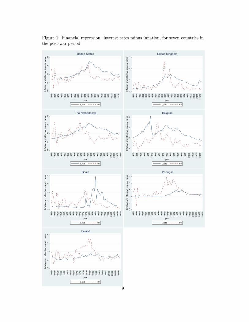
Figure 1: Financial repression: interest rates minus inflation, for seven countries inthe post-war period

−.0

50

.05

.1.1

5In

flatio

n a

nd

eff

ective inte

rest

rate

s

1948

1951

1954

1957

1960

1963

1966

1969

1972

1975

1978

1981

1984

1987

1990

1993

1996

1999

2002

2005

2008

year

i_rate infl

United States

0.1

.2.3

Inflatio

n a

nd

eff

ective inte

rest

rate

s

1946

1949

1952

1955

1958

1961

1964

1967

1970

1973

1976

1979

1982

1985

1988

1991

1994

1997

2000

2003

2006

2009

year

i_rate infl

United Kingdom

−.0

50

.05

.1.1

5In

fla

tio

n a

nd e

ffe

ctive

in

tere

st

rate

s

1948

1951

1954

1957

1960

1963

1966

1969

1972

1975

1978

1981

1984

1987

1990

1993

1996

1999

2002

2005

2008

2011

year

i_rate infl

The Netherlands

0.0

5.1

.15

Infla

tio

n a

nd

effe

ctive inte

rest

rate

s

1955

1958

1961

1964

1967

1970

1973

1976

1979

1982

1985

1988

1991

1994

1997

2000

2003

2006

2009

year

i_rate infl

Belgium

0.1

.2.3

.4In

flatio

n a

nd

eff

ective inte

rest

rate

s

1945

1948

1951

1954

1957

1960

1963

1966

1969

1972

1975

1978

1981

1984

1987

1990

1993

1996

1999

2002

2005

2008

2011

year

i_rate infl

Spain

−.2

−.1

0.1

.2.3

Infla

tio

n a

nd

eff

ective

in

tere

st

rate

s

1945

1948

1951

1954

1957

1960

1963

1966

1969

1972

1975

1978

1981

1984

1987

1990

1993

1996

1999

2002

2005

2008

2011

year

i_rate infl

Portugal

−.2

0.2

.4.6

Infla

tio

n a

nd e

ffe

ctive

in

tere

st

rate

s

1946

1949

1952

1955

1958

1961

1964

1967

1970

1973

1976

1979

1982

1985

1988

1991

1994

1997

2000

2003

2006

2009

year

i_rate infl

Iceland

9

Figure 2: Real growth rates for seven countries in the post-war period

.02

.03

.04

.05

Sm

oo

the

d r

ea

l g

row

th r

ate

s

1948

1951

1954

1957

1960

1963

1966

1969

1972

1975

1978

1981

1984

1987

1990

1993

1996

1999

2002

2005

2008

year

United States

.015.0

2.025.0

3S

mo

oth

ed

rea

l g

row

th r

ate

s

1946

1949

1952

1955

1958

1961

1964

1967

1970

1973

1976

1979

1982

1985

1988

1991

1994

1997

2000

2003

2006

2009

year

United Kingdom.0

2.0

3.0

4.0

5.0

6.0

7S

moo

thed

re

al gro

wth

ra

tes

1948

1951

1954

1957

1960

1963

1966

1969

1972

1975

1978

1981

1984

1987

1990

1993

1996

1999

2002

2005

2008

year

The Netherlands

.01

.02

.03

.04

.05

Sm

ooth

ed

re

al g

row

th r

ate

s

1955

1958

1961

1964

1967

1970

1973

1976

1979

1982

1985

1988

1991

1994

1997

2000

2003

2006

2009

year

Belgium

0.0

2.0

4.0

6.0

8S

mo

oth

ed r

ea

l g

row

th r

ate

s

1945

1948

1951

1954

1957

1960

1963

1966

1969

1972

1975

1978

1981

1984

1987

1990

1993

1996

1999

2002

2005

2008

year

Spain

0.0

2.0

4.0

6S

mo

oth

ed

rea

l g

row

th r

ate

s

1945

1948

1951

1954

1957

1960

1963

1966

1969

1972

1975

1978

1981

1984

1987

1990

1993

1996

1999

2002

2005

2008

year

Portugal

.02

.04

.06

.08

.1S

moo

thed

real gro

wth

rate

s

1946

1949

1952

1955

1958

1961

1964

1967

1970

1973

1976

1979

1982

1985

1988

1991

1994

1997

2000

2003

2006

2009

year

Iceland

10

4 Estimating fiscal reaction functionsOur empirical strategy is straightforward and consists of two main components.First, we calculate the average values for the real interest rates and real growthrates and use these values to obtain 𝛾 from equation (2). Second, we estimateequation (3) for all countries to obtain the fiscal response parameter 𝜌. With bothsets of information we can then estimate 𝛿 as defined in equation (5). Using thisinformation we analyse if government finances have been sustainable and if it wasdue to prudent fiscal policy, financial repression or real growth.

We estimate all the regressions using both OLS and autocorrelation and het-eroskedasticity consistent estimators. We estimate the post-war period16 and weonly present the multivariate regressions including the indicator of fluctuations inincome growth (YVAR) and fluctuations in government expenditures (GVAR) ascontrol variables, given the importance of these two variables for the analysis (cf.Bohn, 1998).17

Analogous to Bohn (2008), we use an HP-filter (𝜆 = 100) to extract the trendcomponent of log real GDP and define YVAR as the gap between the actual valueand this trend in percentage points of GDP.18 For the UK and the US, where militaryspending drives temporary government spending, we define GVAR as the militaryspending-to-GDP ratio. This is comparable to Bohn (2008) who defines GVAR asthe gap between a permanent component of military outlays to GDP from an esti-mated AR(2) process and the actual values. Our approach probably overestimatestemporary military spending by a constant term, which likely has no impact on 𝜌.For all other countries we use the cyclical component of government spending asGVAR, obtained analogously to YVAR.19

These multivariate regressions are the main component of our empirical analysis.However, we also check the robustness of these results. We include the real interestrate as an explanatory variable in equation (3).20 The intuition is that the primarysurplus can also react to changes in real interest rates. First, the government facesless pressure to reduce the debt with fiscal responses, when financial repression isstrong enough to generate negative real interest rates. And second, high real interest

16The estimations for the full sample are presented as a robustness check in Appendix C. We alsoused Bai and Perron (1998, 2003) tests for endogenous structural breaks after the Second WorldWar. The resulting sub-samples, however, are usually too short to estimate a stable fiscal reactionfunction that can assess the long-run institutional stance towards fiscal sustainability. In that case𝜌 picks up short-term policy fluctuations and is not suitable for our analysis.

17The univariate regressions are available upon request.18A more sophisticated way is to estimate potential GDP first and then define the difference

between actual and potential GDP as the output gap. This is used by the OECD (2005). Wedo not apply this method due to data limitations and because the structure of the economy likelychanged over the centuries. In any case, our estimations generate comparable results to those inOECD (2005), so the potential measurement error is probably small.

19Mendoza and Ostry (2008) also use this approach. Their results are robust under a sensitivityanalysis using other specifications.

20 We also included inflation as an additional variable but it was not significant for most regres-sions, and when it was significant it did not change the main results.

11

rates can also force the government to apply fiscal austerity, even when the debt-to-GDP level is not that high. In the case of the US, Bohn (1998) found that interestrates are not a significant control variable.

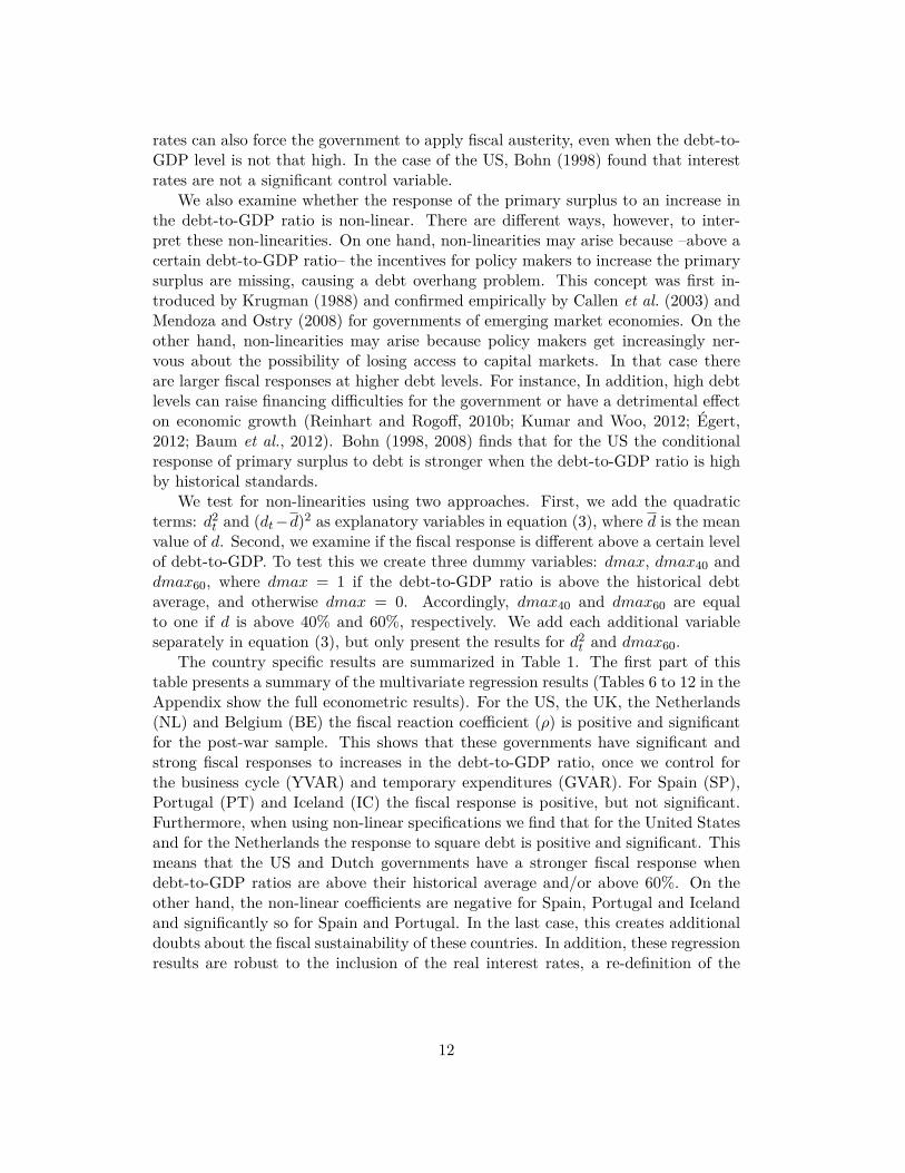
We also examine whether the response of the primary surplus to an increase inthe debt-to-GDP ratio is non-linear. There are different ways, however, to inter-pret these non-linearities. On one hand, non-linearities may arise because –above acertain debt-to-GDP ratio– the incentives for policy makers to increase the primarysurplus are missing, causing a debt overhang problem. This concept was first in-troduced by Krugman (1988) and confirmed empirically by Callen et al. (2003) andMendoza and Ostry (2008) for governments of emerging market economies. On theother hand, non-linearities may arise because policy makers get increasingly ner-vous about the possibility of losing access to capital markets. In that case thereare larger fiscal responses at higher debt levels. For instance, In addition, high debtlevels can raise financing difficulties for the government or have a detrimental effecton economic growth (Reinhart and Rogoff, 2010b; Kumar and Woo, 2012; Égert,2012; Baum et al., 2012). Bohn (1998, 2008) finds that for the US the conditionalresponse of primary surplus to debt is stronger when the debt-to-GDP ratio is highby historical standards.

We test for non-linearities using two approaches. First, we add the quadraticterms: 𝑑2

𝑡 and (𝑑𝑡 −𝑑)2 as explanatory variables in equation (3), where 𝑑 is the meanvalue of 𝑑. Second, we examine if the fiscal response is different above a certain levelof debt-to-GDP. To test this we create three dummy variables: 𝑑𝑚𝑎𝑥, 𝑑𝑚𝑎𝑥40 and𝑑𝑚𝑎𝑥60, where 𝑑𝑚𝑎𝑥 = 1 if the debt-to-GDP ratio is above the historical debtaverage, and otherwise 𝑑𝑚𝑎𝑥 = 0. Accordingly, 𝑑𝑚𝑎𝑥40 and 𝑑𝑚𝑎𝑥60 are equalto one if 𝑑 is above 40% and 60%, respectively. We add each additional variableseparately in equation (3), but only present the results for 𝑑2

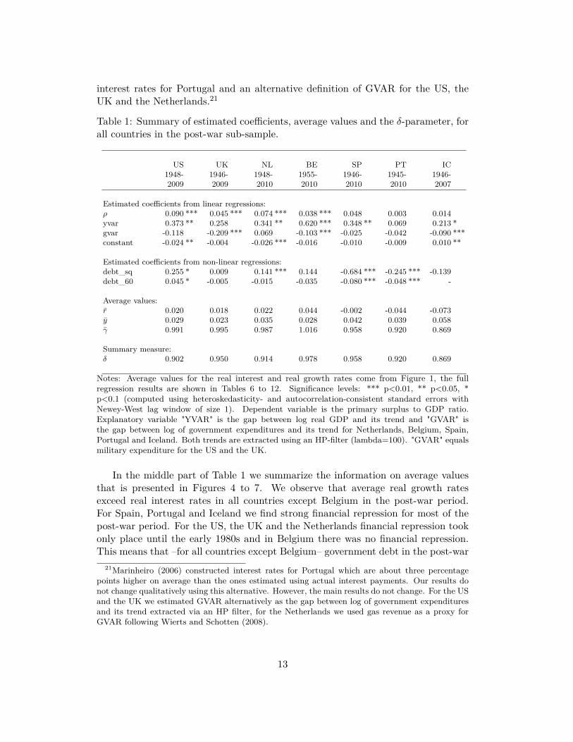
𝑡 and 𝑑𝑚𝑎𝑥60.The country specific results are summarized in Table 1. The first part of this

table presents a summary of the multivariate regression results (Tables 6 to 12 in theAppendix show the full econometric results). For the US, the UK, the Netherlands(NL) and Belgium (BE) the fiscal reaction coefficient (𝜌) is positive and significantfor the post-war sample. This shows that these governments have significant andstrong fiscal responses to increases in the debt-to-GDP ratio, once we control forthe business cycle (YVAR) and temporary expenditures (GVAR). For Spain (SP),Portugal (PT) and Iceland (IC) the fiscal response is positive, but not significant.Furthermore, when using non-linear specifications we find that for the United Statesand for the Netherlands the response to square debt is positive and significant. Thismeans that the US and Dutch governments have a stronger fiscal response whendebt-to-GDP ratios are above their historical average and/or above 60%. On theother hand, the non-linear coefficients are negative for Spain, Portugal and Icelandand significantly so for Spain and Portugal. In the last case, this creates additionaldoubts about the fiscal sustainability of these countries. In addition, these regressionresults are robust to the inclusion of the real interest rates, a re-definition of the

12

interest rates for Portugal and an alternative definition of GVAR for the US, theUK and the Netherlands.21

Table 1: Summary of estimated coefficients, average values and the 𝛿-parameter, forall countries in the post-war sub-sample.

US UK NL BE SP PT IC1948-2009

1946-2009

1948-2010

1955-2010

1946-2010

1945-2010

1946-2007

Estimated coefficients from linear regressions:𝜌 0.090 *** 0.045 *** 0.074 *** 0.038 *** 0.048 0.003 0.014yvar 0.373 ** 0.258 0.341 ** 0.620 *** 0.348 ** 0.069 0.213 *gvar -0.118 -0.209 *** 0.069 -0.103 *** -0.025 -0.042 -0.090 ***constant -0.024 ** -0.004 -0.026 *** -0.016 -0.010 -0.009 0.010 **

Estimated coefficients from non-linear regressions:debt_sq 0.255 * 0.009 0.141 *** 0.144 -0.684 *** -0.245 *** -0.139debt_60 0.045 * -0.005 -0.015 -0.035 -0.080 *** -0.048 *** -

Average values:𝑟 0.020 0.018 0.022 0.044 -0.002 -0.044 -0.073𝑦 0.029 0.023 0.035 0.028 0.042 0.039 0.058𝛾 0.991 0.995 0.987 1.016 0.958 0.920 0.869

Summary measure:𝛿 0.902 0.950 0.914 0.978 0.958 0.920 0.869

Notes: Average values for the real interest and real growth rates come from Figure 1, the fullregression results are shown in Tables 6 to 12. Significance levels: *** p<0.01, ** p<0.05, *p<0.1 (computed using heteroskedasticity- and autocorrelation-consistent standard errors withNewey-West lag window of size 1). Dependent variable is the primary surplus to GDP ratio.Explanatory variable "YVAR" is the gap between log real GDP and its trend and "GVAR" isthe gap between log of government expenditures and its trend for Netherlands, Belgium, Spain,Portugal and Iceland. Both trends are extracted using an HP-filter (lambda=100). "GVAR" equalsmilitary expenditure for the US and the UK.

In the middle part of Table 1 we summarize the information on average valuesthat is presented in Figures 4 to 7. We observe that average real growth ratesexceed real interest rates in all countries except Belgium in the post-war period.For Spain, Portugal and Iceland we find strong financial repression for most of thepost-war period. For the US, the UK and the Netherlands financial repression tookonly place until the early 1980s and in Belgium there was no financial repression.This means that –for all countries except Belgium– government debt in the post-war

21Marinheiro (2006) constructed interest rates for Portugal which are about three percentagepoints higher on average than the ones estimated using actual interest payments. Our results donot change qualitatively using this alternative. However, the main results do not change. For the USand the UK we estimated GVAR alternatively as the gap between log of government expendituresand its trend extracted via an HP filter, for the Netherlands we used gas revenue as a proxy forGVAR following Wierts and Schotten (2008).

13

period was made sustainable as a result of financial repression (for part or the wholeperiod), and thus, strong fiscal responses were not required in most countries.

Finally, in the bottom part of Table 1 we present the 𝛿-parameter, which com-bines the regression results of the FRF with the historical averages. Recall thatgovernment finances are deemed sustainable if 𝛿 = 𝛾(1 − 𝜌) < 1. If 𝜌 is significantlypositive and 𝜌 > (𝛾 − 1)/𝛾 then debt-to-GDP ratios are sustainable due to fiscalresponsibility. If 𝛾 < 1 then this can be due to financial repression, the growthdividend, or a combination of both. From Table 1 we find that this parameter issmaller than one for all countries, implying debt sustainability. However, these post-war results do not assure that debt is or will be sustainable for all these countriesin the near future. In particular, with the end of financial repression, which is noteven feasible for members of the European monetary union, the importance of fis-cal responses has greatly increased. Therefore, those countries with non-significant𝜌 parameters may have difficulties to maintain debt-to-GDP ratios at sustainablelevels. This is made clear by analysing the behaviour of interest rates after the1980s, when financial repression ended for most countries in our sample (see Table2). Hence, the increase in real interest rates increases 𝛾 substantially and makes itnecessary to have a strong fiscal response to keep government debt under control.Moreover, the absence of a linear fiscal response, in conjunction with a negativequadratic fiscal response for Spain, Portugal and Iceland rises the concern that debtmay not be sustainable in these countries.

Table 2: Average interest rates, growth rates and 𝛾-parameter for 1987-2010.

US UK NL BE SP PT IC

𝑟 0.039 0.044 0.046 0.043 0.077 -0.002 0.022𝑦 0.026 0.022 0.025 0.021 0.032 0.027 0.038𝛾 1.012 1.021 1.020 1.022 1.044 0.972 0.984

5 Stochastic debt sustainability indicatorsThe probability distribution of future debt levels is important in assessing fiscalsustainability. Higher interest and growth rate volatility increases the distribution offuture debt levels and requires a larger fiscal response to keep government debt undercontrol. To assess this relationship we extend the results in the previous section –where we used a simple historical average for 𝛾– by simulating future interest andgrowth rate values, which in turn provide a probability distribution for future debt-to-GDP levels. We insert the simulated interest and growth rates into equation (4)and use that 𝐸(Zt) = 𝐸(𝜀𝑡) = 0 by construction.

𝑑𝑡+1 = 𝛾𝑡(1 − 𝜌)𝑑𝑡 − 𝛾𝑡𝛼, (6)

14

The expected steady state future debt level can be obtained by writing equation (6)as a differential equation as in Haselmann et al. (2002):

Δ𝑑𝑡+1 = − [1 − 𝛾(1 − 𝜌)] 𝑑𝑡 − 𝛾𝛼, (7)

and solving for its steady state. The stationarity conditions are those from Section 2.For 𝛿 > 1 no stable condition exists, while for 𝛿 < 1 debt is stationary and convergestowards 𝑑 = (1 − 𝛾(1 − 𝜌))−1 𝛾𝛼. For 𝛼 > 0 the stabilizing debt level is negative(i.e. in the long run this government will have more assets than liabilities) andfor 𝛼 < 0 the stabilizing debt level is positive. All the countries in our stochasticanalysis converge towards a stable positive debt level with 𝛾 from Table 2 and 𝜌and 𝛼 from Table 1.22 For 𝜌 = 0 only Portugal and Iceland have a stationarydebt level. Divergence occurs slow however, only the UK and Spain present clearlyexplosive debt paths when 𝜌 = 0. When we set 𝜌 = 0 in our simulations below weuse 𝛼 equals the average primary surplus ps. Changing the constant increases theprojected median debt-to-GDP ratios at any given future date, with the Netherlandsbeing the only exception. This occurs because the fiscal reaction coefficient reactsto both increases and reductions of the debt level from its long-run average.23

In simulating interest and growth rate volatility, we follow Budina and van Wi-jnbergen (2008) and use a stochastic two variable VAR model for real interest andgrowth rates to capture the historic volatility of interest and growth rates:(︃

𝑟𝑡

𝑦𝑡

)︃= 𝛼0 +

∞∑︁𝑗=1

𝐴𝑗

(︃𝑟𝑡−𝑗

𝑦𝑡−𝑗

)︃+ 𝜂𝑡, (8)

var (𝜂𝑡) = Σ.

In this set-up shocks to real interest and growth rates are not correlated over timebut are correlated within the same time period.24 We run the simulations 10.000times to obtain a debt path from 2010 to 2029 for two scenarios: one with 𝜌 = 0and another with 𝜌 > 0.25 For the US, UK, Netherlands and Belgium, which havepositive and significant 𝜌 coefficients we use the post-war coefficient values. For

22Iceland is an exception, it converges towards a negative debt level.23The Netherlands had a relatively stable debt level of around 60% of GDP in the post-war

period (see Figure 5 in the Appendix) and without a fiscal response its median projected debt levelis declining steeply (due to the steady-state long-term conditions given by changes in 𝑟 and 𝑦).Hence, the inclusion of the fiscal response "stabilizes" its debt level around its post-war average of60%, and this results in the projected median debt level being lower with 𝜌 = 0 than with 𝜌 > 0.

24Equation (8) is estimated for each country using 1987 as a starting point. In this way weavoid using the historically low real interest rates levels when financial repression was present. Theexception is Belgium for which we used historical debt and primary surplus from the post-warsample since it was the only country in our sample that did not rely on financial repression to makeits fiscal policy sustainable post-war and Belgian debt peaked in 1987, so post-1987 data gives askewed impression. In addition, we set the number of lags in equation (8) to two following theAkaike information criterion.

25For time 𝑡 + 1 we insert the realizations of time 𝑡 and the shocks of time 𝑡 + 1 into equations(6) and (8), for time 𝑡 + 2 we use the just simulated realizations of time 𝑡 + 1 and the shocks of time𝑡 + 2 as inputs and so on and so forth.

15

Spain, Portugal and Iceland, which did not have significant 𝜌 coefficients in thepost-war sample, we use 𝜌 = 0.04 for illustrative purposes. The 95% and 99% debtquantiles are plotted in fan charts in Figures 8 and 9 in the Appendix.

In equation (6) fiscal policy for 𝜌 > 0 responds to a deviation in the debt levelfrom 𝑑, which is its historical average. Shocks in interest and growth rates thatdrive the debt level away from 𝑑 are thus in the subsequent period countered by afiscal response. Similarly, shocks that drive the debt level towards 𝑑 are mitigatedby a smaller fiscal response. This effect is stronger if 𝜌 is bigger relative to theinterest and growth rate volatility. We observe this from From Figures 8 and 9 inthe Appendix. The debt levels have relatively small 90% and 95% confidence bandsfor the first set of countries: the US, UK, Netherlands and Belgium. For the secondgroup –Spain, Portugal and Iceland– these confidence bands are larger. From Figure9 it is clear that the imposed values of 𝜌 = 0.04 are not sufficiently large for Spain,Portugal and Iceland.

A positive and significant fiscal response has two main effects on our debt projec-tions. First, it directly contributes to sustainable fiscal policy by lowering expectedfuture debt levels. Second, it reduces the impact of uncertainty on interest andgrowth rates, which results in narrower confidence bands. To indicate both we de-velop a debt sustainability indicator 𝑋𝑑,𝑗 which is defined as follows:

𝑋𝑑,𝑗 =Σ𝑘𝐼

(︁{𝑑𝑘

𝑡+1, . . . , 𝑑𝑘𝑡+𝑗} > 𝑑

)︁𝑘

, (9)

where 𝐼() = 1 if 𝑑𝑡+𝑖 > 𝑑 for 1 ≤ 𝑖 ≤ 𝑗 and 𝑑𝑘𝑡+𝑗 is simulation number 𝑘. As fixed debt

threshold levels we choose the 60% of the Stability and Growth Pact, which givesthe indicator: 𝑋60,10, and the 90% of Reinhart and Rogoff (2010b) that provides theindicator 𝑋90,10. We also calculated 𝑋+20,10: the probability debt increases morethen 20%-points between a 10-year period (in this case from 2010 to 2019).

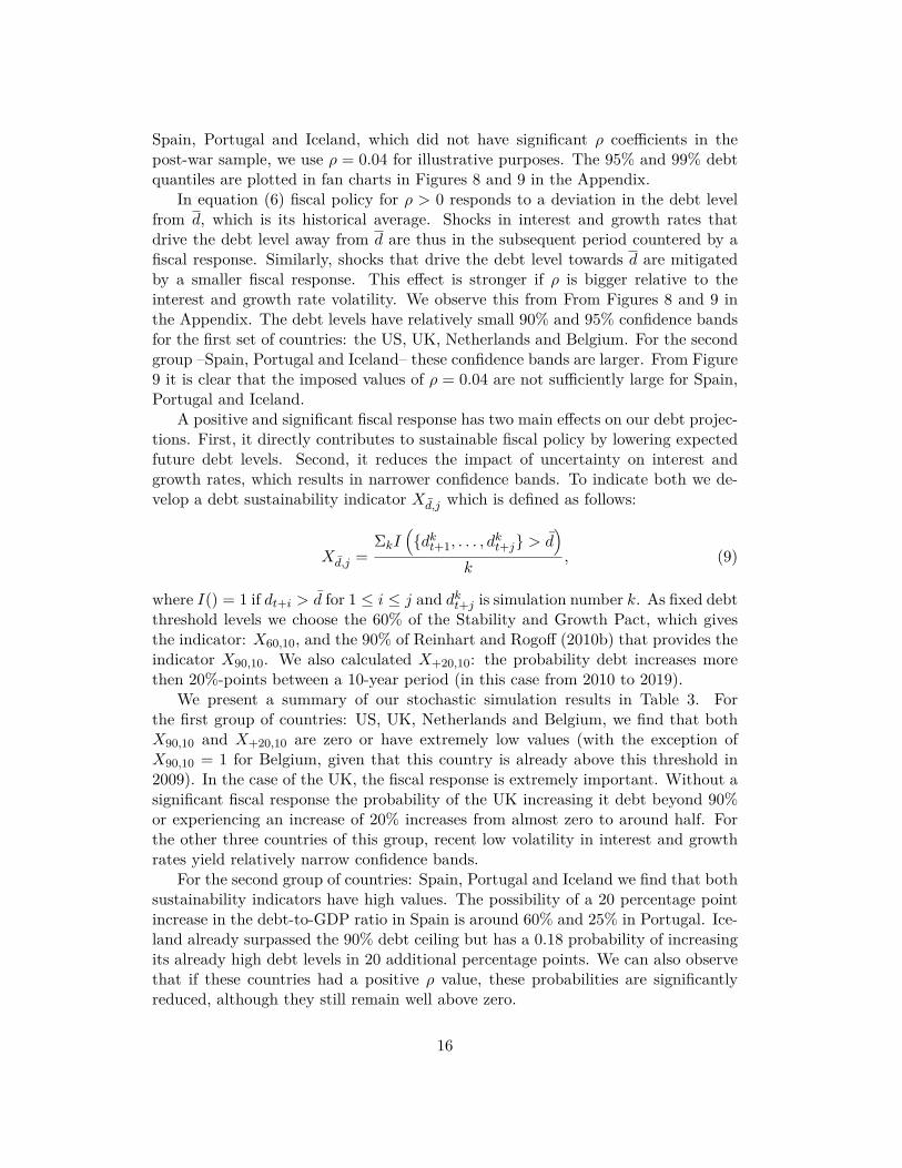
We present a summary of our stochastic simulation results in Table 3. Forthe first group of countries: US, UK, Netherlands and Belgium, we find that both𝑋90,10 and 𝑋+20,10 are zero or have extremely low values (with the exception of𝑋90,10 = 1 for Belgium, given that this country is already above this threshold in2009). In the case of the UK, the fiscal response is extremely important. Without asignificant fiscal response the probability of the UK increasing it debt beyond 90%or experiencing an increase of 20% increases from almost zero to around half. Forthe other three countries of this group, recent low volatility in interest and growthrates yield relatively narrow confidence bands.

For the second group of countries: Spain, Portugal and Iceland we find that bothsustainability indicators have high values. The possibility of a 20 percentage pointincrease in the debt-to-GDP ratio in Spain is around 60% and 25% in Portugal. Ice-land already surpassed the 90% debt ceiling but has a 0.18 probability of increasingits already high debt levels in 20 additional percentage points. We can also observethat if these countries had a positive 𝜌 value, these probabilities are significantlyreduced, although they still remain well above zero.

16

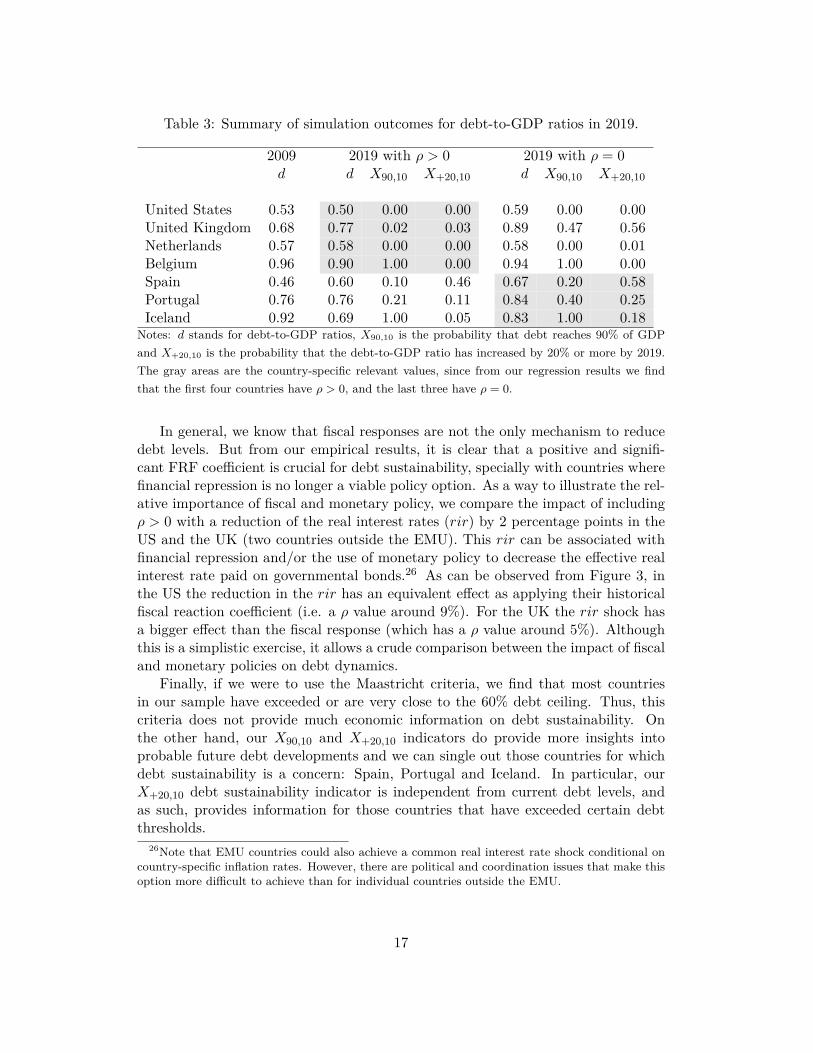
Table 3: Summary of simulation outcomes for debt-to-GDP ratios in 2019.

2009 2019 with 𝜌 > 0 2019 with 𝜌 = 0𝑑 𝑑 𝑋90,10 𝑋+20,10 𝑑 𝑋90,10 𝑋+20,10

United States 0.53 0.50 0.00 0.00 0.59 0.00 0.00United Kingdom 0.68 0.77 0.02 0.03 0.89 0.47 0.56Netherlands 0.57 0.58 0.00 0.00 0.58 0.00 0.01Belgium 0.96 0.90 1.00 0.00 0.94 1.00 0.00Spain 0.46 0.60 0.10 0.46 0.67 0.20 0.58Portugal 0.76 0.76 0.21 0.11 0.84 0.40 0.25Iceland 0.92 0.69 1.00 0.05 0.83 1.00 0.18

Notes: 𝑑 stands for debt-to-GDP ratios, 𝑋90,10 is the probability that debt reaches 90% of GDPand 𝑋+20,10 is the probability that the debt-to-GDP ratio has increased by 20% or more by 2019.The gray areas are the country-specific relevant values, since from our regression results we findthat the first four countries have 𝜌 > 0, and the last three have 𝜌 = 0.

In general, we know that fiscal responses are not the only mechanism to reducedebt levels. But from our empirical results, it is clear that a positive and signifi-cant FRF coefficient is crucial for debt sustainability, specially with countries wherefinancial repression is no longer a viable policy option. As a way to illustrate the rel-ative importance of fiscal and monetary policy, we compare the impact of including𝜌 > 0 with a reduction of the real interest rates (𝑟𝑖𝑟) by 2 percentage points in theUS and the UK (two countries outside the EMU). This 𝑟𝑖𝑟 can be associated withfinancial repression and/or the use of monetary policy to decrease the effective realinterest rate paid on governmental bonds.26 As can be observed from Figure 3, inthe US the reduction in the 𝑟𝑖𝑟 has an equivalent effect as applying their historicalfiscal reaction coefficient (i.e. a 𝜌 value around 9%). For the UK the 𝑟𝑖𝑟 shock hasa bigger effect than the fiscal response (which has a 𝜌 value around 5%). Althoughthis is a simplistic exercise, it allows a crude comparison between the impact of fiscaland monetary policies on debt dynamics.

Finally, if we were to use the Maastricht criteria, we find that most countriesin our sample have exceeded or are very close to the 60% debt ceiling. Thus, thiscriteria does not provide much economic information on debt sustainability. Onthe other hand, our 𝑋90,10 and 𝑋+20,10 indicators do provide more insights intoprobable future debt developments and we can single out those countries for whichdebt sustainability is a concern: Spain, Portugal and Iceland. In particular, our𝑋+20,10 debt sustainability indicator is independent from current debt levels, andas such, provides information for those countries that have exceeded certain debtthresholds.

26Note that EMU countries could also achieve a common real interest rate shock conditional oncountry-specific inflation rates. However, there are political and coordination issues that make thisoption more difficult to achieve than for individual countries outside the EMU.

17

Figure 3: Stochastic median debt projections, for the US and the UK from 2010 to2014 with a real interest shock (𝑟𝑖𝑟 shock), with a positive fiscal reaction (𝜌 > 0)and without (𝜌 = 0)

50%

52%

54%

56%

58%

60%

2009 2010 2011 2012 2013 2014

De

bt/

GD

P

United States

rho=0

rho>0

rir shock

60%

65%

70%

75%

80%

85%

90%

2009 2010 2011 2012 2013 2014

De

bt/

GD

P

United Kingdom

rho=0

rho>0

rir shock

6 Summary and conclusionsUsing historical data on public finances for seven OECD countries, in combinationwith the empirical methodology developed by Bohn (1998, 2008), we identify thethree main channels through which governments can reduce the debt-to-GDP ratio.These case studies lead to the conclusion that using estimated fiscal reaction coef-ficients –in conjunction with the viability of a country to apply financial repressionand/or increases average real growth rates– provides crucial information to assessdebt sustainability. These fiscal reaction coefficients reflect country-specific insti-tutions and attitudes towards debt sustainability that are essential to understandtheir prospects to effectively reduce debt levels in the medium term. In doing so, itis necessary to take a sufficiently long time period and to examine the existence ofnon-linearities.

We find that four countries: the US, UK, Netherlands and Belgium have persis-tently positive and significant fiscal reaction coefficients, conditional on temporarygovernment spending (e.g. war expenditure) and cyclical economic fluctuations.These strong fiscal responses are found in both the full sample and also in the post-war period. Together with average moderate real growth rates (and high rates insome countries for some periods) and financial repression, these countries have expe-rienced sustainable debt-to-GDP ratios over time. In particular, from the end of theSecond World War to around the mid-1970s, the use of effective financial repressionmechanisms in these countries allowed for drastic reductions in the debt-to-GDPratio, which had reached significantly high levels due to military expenditures dur-ing the Second World War (specially in the US and UK). After the mid-1970s withthe end of financial repression and lower real growth rates, these countries reliedincreasingly on fiscal responsibility (i.e. moderate primary surplus to GDP ratios)to maintain debt at sustainable levels. The role of fiscal policy has become evenmore important for those countries that belong to the euro area, and which do not

18

have autonomous monetary or exchange rate policies. Debt sustainability in thesecountries is clearly reflected in the extremely low values in our 𝑋+20,10 indicator.

On the other hand, for Spain, Portugal and Iceland, we do not find significantfiscal reaction coefficients. With the end of financial repression, this means thatthese countries are less prepared to maintain sustainable debt levels in the future.Our debt sustainability indicators: 𝑋+20,10 and 𝑋90,10 clearly identify this weaknessin the debt dynamics of these countries by providing large positive probabilities(sometimes above 50%).

ReferencesAfonso, A. (2005). “Fiscal Sustainability: The Unpleasant European Case”, Finan-

zArchiv 61(1): 19–44.

Bai, J. and Perron, P. (1998). “Estimating and Testing Linear Models with MultipleStructural Changes”, Econometrica 66(1): 47–78.

Bai, J. and Perron, P. (2003). “Computation and Analysis of Multiple StructuralChange Models”, Journal of Applied Econometrics 18(1): 1–22.

Barro, R. J. (1979). “On the Determination of Public Debt”, Journal of PoliticalEconomy 87(5): 940–971.

Baum, A., Checherita-Westphalz, C. and Rotherix, P. (2012). “Debt and Growth:New Evidence for the Euro Area”. ECB mimeo.

Bi, H. (2011). “Sovereign Default Risk Premia, Fiscal Limits and Fiscal Policy”,Discussion Paper.

Bohn, H. (1991). “Budget balance through revenue or spending adjustments?:Some historical evidence for the United States”, Journal of Monetary Economics27(3): 333–359.

Bohn, H. (1998). “The Behavior of U.S. Public Debt and Deficits”, Quarterly Journalof Economics 113(3): 949–963.

Bohn, H. (2007). “Are Stationary and Cointegration Restrictions Really Neces-sary for the Intertemporal Budget Constraing?”, Journal of Monetary Economics54(7): 1837–1847.

Bohn, H. (2008). “The Sustainability of Fiscal Policy in the United States”, inR. Neck and J. Sturm (eds.), Sustainability of Public Debt, MIT Press, pp. 15–49.

Bos, F. (2007). “The Dutch fiscal framework; history, current practice and the roleof the CPB”, CPB Discussion Paper 150.

Brender, A. and Drazen, A. (2005). “Political budget cycles in new versus establisheddemocracies”, Journal of Monetary Economics 52(7): 1271–1295.

19

Brender, A. and Drazen, A. (2008). “How Do Budget Deficits and Economic GrowthAffect Reelection Prospects? Evidence from a Large Panel of Countries”, Ameri-can Economic Review 98(5): 2203–20.

Budina, N. and van Wijnbergen, S. (2008). “Quantitative Approaches to FiscalSustainability Analysis: A Case Study of Turkey since the Crisis of 2001”, WorldBank Economic Review 23(1): 119–140.

Callen, T., Terrones, M., Debrun, X., Daniel, J. and Allard, C. (2003). “Public Debtin Emerging Markets: Is is Too High?”, World Economic Outlook, InternationalMonetary Fund, chapter III.

CBS (1959). “Zestig jaren statistiek in tijdreeksen (1899-1959)”.

CBS (1994). “Vijfennegentig jaren statistiek in tijdreeksen (1899-1994)”.

CBS (2001). “Tweehonderd jaar statistiek in tijdreeksen (1800-1999)”.

Comín, F. and Díaz, D. (2005). “Sector Público Administrativo y Estado del Bien-estar”, in A. Carreras and X. Tafunell (eds.), Estadísticas Históricas de España:Siglos XIX y XX, 2nd edition edn, Fundación BBVA, Bilbao, Spain, pp. 873–964.

De Paoli, B., Hoggarth, G. and Saporta, V. (2009). “Output costs of sovereigncrises: some empirical estimates”, Bank of England working papers 362, Bank ofEngland.

Égert, B. (2012). “Public finances and economic growth in the long run: evidencefrom non-linear Bayesian model averaging”. OECD mimeo.

European Commission (2009). “Sustainability Report 2009”, European Economy 9/ 2009, Directorate-General for Economic and Financial Affairs (DG EcFin).

Furceri, D. and Zdzienicka, A. (2011). “How Costly Are Debt Crises?”, IMF WorkingPapers 11/280, International Monetary Fund.

Ghosh, A. R., Kim, J. I., Mendoza, E. G., Ostry, J. D. and Qureshi, M. S. (2011).“Fiscal Fatigue, Fiscal Space and Debt Sustainability in Advanced Economies”,NBER Working Papers 16782, National Bureau of Economic Research, Inc.

Haselmann, R., Holle, S., Kool, C. and Ziesemer, T. (2002). “Sovereign Risk andSimple Debt Dynamics: The Case of Brazil and Argentina”, Research Memoranda034, Maastricht : MERIT, Maastricht Economic Research Institute on Innovationand Technology.

Krugman, P. R. (1988). “Financing vs. Forgiving a Debt Overhang”, Journal ofDevelopment Economics 29(3): 253–268.

Kumar, M. S. and Woo, J. (2012). “Public debt and growth”. IMF mimeo.

20

Maddison, A. (2003). The World Economy, historical satistics, OECD, DevelopmentCentre Studies, Paris, France.

Marinheiro, C. F. (2006). “The Sustainability of Portuguese Fiscal Policy from aHistorical Perspective”, Empirica 33(2-3): 155–179.

Mendoza, E. G. and Ostry, J. D. (2008). “International evidence on fiscal solvency:Is fiscal policy "responsible"?”, Journal of Monetary Economics 55(6): 1081–1093.

Michell, B. R. (1988). British historical statistics, Cambridge University Press,Cambridge, UK.

OECD (2005). “Measuring Cyclically-adjusted Budget Balances for OECD Coun-tries”, OECD Working Paper 434.

Peacock, A. T. and Wiseman, J. (1961). The Growth of Public Expenditure in theUnited Kingdom, number peac61-1 in NBER Books, National Bureau of EconomicResearch, Inc.

Pirard, J. (1999). L’extension du r ole de l’Etat en Belgique aux XIXe et XXesiècles, publisher, Brussel, Belgium.

Polito, V. and Wickens, M. (2012). “A model-based indicator of the fiscal stance”,European Economic Review 56(3): 526 – 551.

Prados de la Escosura, L. (2003). El Progreso Económico de España (1850-2000),Fundación BBVA, Bilbao, Spain.

Reinhart, C. M. and Rogoff, K. S. (2008). “This Time is Different: A PanoramicView of Eight Centuries of Financial Crises”, NBER Working Paper 13882, Na-tional Bureau for Economic Research.

Reinhart, C. M. and Rogoff, K. S. (2010a). “From Financial Crash to Debt Crisis”,NBER Working Paper 15795, National Bureau for Economic Research.

Reinhart, C. M. and Rogoff, K. S. (2010b). “Growth in a Time of Debt”, WorkingPaper 15639, National Bureau of Economic Research.

Reinhart, C. M. and Sbrancia, M. B. (2011). “The Liquidation of GovernmentDebt”, NBER Working Paper 16893, National Bureau for Economic Research.

Sturzenegger, F. and Zettelmeyer, J. (2007). Debt Defaults and Lessons from aDecade of Crises, Vol. 1, 1 edn, The MIT Press.

van Zanden, J. L. (1996). “The development of Government Finances in a chaoticperiod, 1807-1850”, Economic and Social History in the Netherlands 7: 53–71.

Wierts, P. and Schotten, G. (2008). “De Nederlandse gasbaten en het begrotings-beleid: theorie versus praktijk”, DNB Occasional Studies 6(5).

21

Appendix

A Data sources and pre-processingUnder the subsequent country headings we describe our data sources, elaborate onthe definitions used (general/central government) and whether breaks in the dataare present. Table 4 presents a summary of the available data for each country.

Table 4: Available data per country

Country Samples ObservationsUS 1792-2009 218UK 1691-2009 319Netherlands 1816-1939 1948-2009 186Belgium 1830-1913 1919-1939 1955-2009 158Spain 1850-1935 1940-2010 157Portugal 1852-2010 159Iceland 1908-2010 103

In Figures 4-7 we plot the debt-to-GDP ratio, the primary surplus to GDPratio, a smoothed series of interest minus growth rate and for the UK and the USthe GVAR indicator.

As the effective interest rate we use the simple formula: 𝑖𝑒𝑡 = 𝑖𝑝𝑡/𝑑𝑡−1 where 𝑖𝑒

is the effective interest rate and 𝑖𝑝 is interest payment on debt 𝑑, both in nominalterms.27

United States

We use the data from Bohn (2008) from 1792-2009.28 This is a continuous dataseton nominal and real GDP, government gross debt, government primary surplus,government interest expenditure and government military expenditure. A detaileddescription of the data used there can be found in Bohn (1991) and Bohn (2008),and references therein.

Government military expenditure is used as an indicator for temporary govern-ment spending GVAR as government expenditure in wartime is significantly differentfrom government spending in peacetime. Using dummy variables for the war years29

instead of actual military expenditure does not change the results significantly.27This simple formula is almost perfectly correlated (0.9975) with a more precise specification

given by: 𝑖𝑒𝑡 = 𝑖𝑝𝑡

2

(︃𝑑𝑡(︀

𝑝𝑡𝑝𝑡−1

)︀ 12

+ 𝑑𝑡−1(︀𝑝𝑡

𝑝𝑡−1

)︀ 12

)︃−1

where 𝑝 is the GDP deflator.

28Henning Bohn kindly provided us with an updated database which runs until 2009. He usedthe 2011 Budget of the United States for this update.

291812-1815 War of 1812, 1846-1849 (Mexican-American War), 1861-1865 (American Civil War),1917-1920 (World War I), 1940-1945 (World War II)

22

UK

The sample from the UK is from 1692-2010 with a break in 1800 and in 1946. Thereis a shift in the reporting year in 1800, prior to 1946 we use central governmentdata and after 1946 we use general government data. We use military expenditureas a proxy for temporary government spending and there is a break in this series in1980 probably due to a different specification. Prior to 1946 military expenditureand interest expenditure are the only two large items on the central governmentsbudget. Non-military non-interest spending never exceeds 2% of GDP.30 Data isobtained from six sources:

∙ Data on central government expenditure (1692-1945), interest expenditure(1692-1945), military expenditure (1692-1980), revenue (1692-1946), publicdebt (1692-1979), CPI as a proxy for the GDP deflator (1691-1792), a GDPdeflator (1830-1946) and nominal GDP (1830-1946) has been obtained fromMichell (1988).

∙ From Peacock and Wiseman (1961) real and nominal GDP is obtained for theyears 1792, 1800, 1814, 1822, 1831. Constant growth rates in real and nominalGDP are assumed between these dates.

∙ Real GDP for 1700 and 1800 is obtained from Maddison (2003) world historictables. Constant growth rates in real GDP is assumed between 1700 and 1792and in the period 1691-1700.

∙ General government expenditure, interest expenditure, revenue and real andnominal GDP from 1946 onwards is obtained from the Office of National Statis-tics

∙ Public debt is obtained from the UK Ministry of Finance for 1980-2010

∙ Military expenditure for 1980-2010 is obtained from the OECD.

A GDP deflator and real GDP from 1692-2010 is obtained by coupling the variouspartial GDP series with each other. Furthermore GDP has been adjusted suchthat Ireland is excluded prior to 1920 as it is after 1920. Temporary governmentexpenditure GVAR is military spending. As an alternative we use gap between thelog of government expenditure and its trend.

Netherlands

Data is obtained from Bos (2007) and contains nominal GDP, a piecewise continuousGDP deflator, gross government debt and a decomposition of government revenueand government expenditure in their main components. It runs from 1815 till 2009with gaps in the inter-war years. Bos acquires data on general government finances

30Except for 1836 and 1837. In these years the government compensated slave owners for out-lawing slavery.

23

in the period 1815-1900 from the work of van Zanden (1996) and from 1900 on-wards from Statistics Netherlands. In the period 1850-1900 only data on centralgovernment finances are available. Furthermore data on local government interestexpenditure is missing until 1947.

We correct for that by using two assumptions. First, we assume that the interestrate on non-central government debt equals the interest rate on central governmentdebt. In the Netherlands, the central government steps in and assumes full liabilitywhen local governments are in financial distress. Therefore local government de-fault risk is equal to central government default risk. Second we assume that localgovernment finances have run a balanced budget, as they are required by law, andwe interpolate non-central government debt between 1850 and 1900 linearly. Thisseems a reasonable first assumption as in 1850 non-central government debt is 26.0%of general government debt, in 1900 it is 20.2%. If these assumptions underestimatelocal interest expenditure, primary surplus and implied interest rates prior to 1947would be lower than their actual value. The effect on debt sustainability will beabsent, as primary surplus and the implied interest rates have opposite signs in theaccounting equation. This has been tested by using central instead of general gov-ernment finances. As none of the regression coefficients except for the constant tochanged by more than one standard deviation, we deem these assumptions reason-able.

Bos (2007) provides GDP deflators from 1815-1913, 1921-1939 and 1948-2009,Statistics Netherlands (CBS, 1959, 1994, 2001) provides a consumer price index from1900-2009. A continuous GDP deflator is constructed by using consumer price in-dices to bridge the gap between the broken piece-wise continuous GDP deflators. Weapproximate the GDP deflator from 1913-1921 and from 1939-1948 by the consumerprice index. The consumer price index is highly correlated with the GDP deflatorin the period 1900-1913, 1922-1939 and 1949-2009: correlation is 0.998 on level and0.949 on first differences.

Temporary government expenditure is defined as the residual of government ex-penditure after its HP-filtered mean has been removed. Note that Bohn (2008) usesmilitary expenditure as an alternative measure of temporary government expendi-ture. Unlike the US, where military spending drives government spending prior to1948, the only notable Dutch event is the Belgian war of independence in 1830.Wierts and Schotten (2008) argue gas revenue should be used from 1970s onwardsas it had considerable impact in budgetary policy. Both alternative specificationsare used in robustness checks and do not provide significant changes.

Belgium

The sample from Belgium is from 1830-1913, 1920-1939 and 1955-2010 with a breakin 1970. Prior to 1970 central government data is used, after 1970 general govern-ment data. Data for Belgium has been obtained from 4 sources:

∙ A dataset on Belgium’s central government finances from the independence ofthe state in 1830 until the first world war (1913) was created by Joseph Pi-

24

rard and published in Pirard (1999). He reports central government revenue,expenditure, gross government debt, interest expenditure nominal GDP from1830 onwards. In this book Pirard also publishes this data for the Inter bellum(1920-1939) and the years after the Second World War (1945-1995), which heobtains from other sources. finance data after 1945 as the increase in debt isalways smaller than the difference between government revenue and govern-ment expenditure and much to persistent to be due to stock-flow adjustments.This might be due to the fact that some government bond redemptions areclassified as government expenditure.

∙ Real GDP for the period 1830-1960 is obtained from Maddison (2003) worldhistoric tables. For the years 1831-1839 no data is available here and thus aconstant increase between 1830 and 1840 is assumed.

∙ Data on central government finances (revenue from 1955 until 1970 is obtainedfrom the annual reports of the NBB, the Belgian central bank.

∙ From 1970 onwards data on general government finances and GDP is availablefrom the AMECO database of the European Commission.

The nominal GDP estimates of Pirard are in the period 1970-1995 approximately13% lower than the AMECO data. We correct for this by increasing every data-pointin the nominal GDP series of Pirard by 13%. Temporary government expenditureGVAR is determined as the gap between the log of government expenditure and itstrend.

Spain

The sample is from 1850 to 2010 with a gap for the Spanish Civil War (1936-1939).Data prior to 1995 is taken from Prados de la Escosura (2003) for GDP data inreal and nominal terms and Comín and Díaz (2005) for the public sector data andconcerns national and provincial government finances. After 1995 data is obtainedfrom the AMECO database of the European Commission.

Temporary government expenditure GVAR is determined as the gap betweenthe log of government expenditure and its trend.

Portugal

The sample is from 1850 to 2010. Data comes from Marinheiro (2006) for the period1852-1995. In the statistical appendix to that paper Marinheiro describes the sourcesfrom which he obtains his data. This is a continuous dataset on nominal and realGDP, government gross debt, government primary surplus and government interestexpenditure. The government finances are on cash basis. After 1995 data is obtainedfrom the AMECO database of the European Commission.

Temporary government expenditure GVAR is determined as the gap between thelog of government expenditure and its trend. Portugal defaulted on its governmentdebt in 1892, which was ultimately resolved in 1902.

25

Iceland

The sample for Iceland is from 1908-2010. Data for Iceland has been obtainedfrom two sources. A since 2000 defunct Icelandic organization "Þjóðhagsstofnun’"published general government revenue, expenditure, gross government debt, interestexpenditure and real and nominal GDP from 1908 until 1999. Iceland statisticspublishes data on general government revenue, expenditure, gross government debt,interest expenditure and real and nominal GDP from 1945 onwards. The databetween 1945 and 1999 is identical to the data on the "Þjóðhagsstofnun" website.

Icelandic data concerns general government and contains long periods of highinflation. Temporary government expenditure GVAR is determined as the gap be-tween the log of government expenditure and its trend. Iceland sought and receivedassistance from the IMF and the Scandinavian countries after the 2008 banking cri-sis turned into a sovereign debt crisis for Iceland. This is considered as a public debtdefault.

26

B Descriptive statistics and graphs

Table 5: Summary statistics and correlation coefficients

N mean sd min max ps debt yvar gvar milUS ps 62 0.00 0.02 -0.09 0.06 1.00

debt 62 0.42 0.13 0.24 0.84 0.30 1.00yvar 62 -0.00 0.02 -0.07 0.03 0.12 -0.52 1.00gvar 62 -0.58 0.01 -0.59 -0.53 0.17 0.42 -0.22 1.00mil 62 0.08 0.03 0.04 0.16 0.03 0.39 -0.06 0.50 1.00rir 62 0.02 0.03 -0.06 0.09 -0.22 -0.17 0.05 -0.44 -0.41

UK ps 65 0.02 0.03 -0.05 0.10 1.00debt 65 0.78 0.53 0.33 2.36 0.51 1.00yvar 65 -0.00 0.02 -0.07 0.05 -0.63 -0.51 1.00gvar 65 -0.01 0.06 -0.23 0.10 0.06 -0.42 0.02 1.00mil 65 0.05 0.05 0.03 0.43 0.05 0.60 -0.19 -0.39 1.00rir 65 0.02 0.04 -0.12 0.09 -0.23 -0.48 0.23 0.05 -0.26

N mean sd min max ps debt yvar gvar rirNL ps 62 0.03 0.03 -0.01 0.19 1.00

debt 62 0.67 0.26 0.38 1.65 0.83 1.00yvar 62 0.00 0.03 -0.04 0.09 0.65 0.47 1.00gvar 62 0.02 0.10 -0.10 0.59 0.78 0.73 0.63 1.00rir 62 0.02 0.04 -0.08 0.10 -0.37 -0.19 -0.46 -0.33 1.00

BE ps 56 0.02 0.03 -0.07 0.07 1.00debt 56 0.86 0.30 0.45 1.34 0.34 1.00yvar 56 0.00 0.03 -0.03 0.11 0.04 -0.26 1.00gvar 56 0.03 0.15 -0.21 0.70 -0.21 -0.18 0.73 1.00rir 56 0.04 0.03 -0.04 0.11 0.20 0.16 -0.31 -0.25 1.00

SP ps 65 0.00 0.03 -0.09 0.09 1.00debt 65 0.31 0.13 0.08 0.61 0.17 1.00yvar 65 -0.00 0.03 -0.09 0.05 0.34 -0.20 1.00gvar 65 -0.01 0.08 -0.21 0.21 -0.17 -0.08 -0.19 1.00rir 65 0.00 0.09 -0.16 0.32 0.39 0.32 -0.19 0.19 1.00

PT ps 66 -0.01 0.02 -0.07 0.03 1.00debt 66 0.35 0.20 0.13 0.83 0.01 1.00yvar 66 -0.00 0.04 -0.11 0.10 0.15 -0.06 1.00gvar 66 0.00 0.09 -0.24 0.22 -0.20 0.11 -0.12 1.00rir 66 -0.04 0.06 -0.23 0.18 0.31 0.19 0.23 0.03 1.00

IC ps 65 0.01 0.03 -0.10 0.08 1.00debt 65 0.26 0.20 0.03 0.97 -0.22 1.00yvar 65 -0.00 0.05 -0.13 0.10 0.07 -0.18 1.00gvar 65 0.01 0.13 -0.18 0.39 -0.34 -0.05 0.60 1.00rir 65 -0.05 0.09 -0.26 0.18 0.07 0.35 0.22 0.07 1.00

27

Figure 4: United States and United Kingdom: Debt, primary surplus and militaryexpenditure ratios to GDP, and gamma parameter, post-war samples

.2.4

.6.8

De

bt

/ G

DP

1948

1951

1954

1957

1960

1963

1966

1969

1972

1975

1978

1981

1984

1987

1990

1993

1996

1999

2002

2005

2008

year

United States

.51

1.5

22.5

De

bt

/ G

DP

1946

1949

1952

1955

1958

1961

1964

1967

1970

1973

1976

1979

1982

1985

1988

1991

1994

1997

2000

2003

2006

2009

year

United Kingdom

−.1

−.0

50

.05

.1P

rim

ary

Su

rplu

s /

GD

P

1948

1951

1954

1957

1960

1963

1966

1969

1972

1975

1978

1981

1984

1987

1990

1993

1996

1999

2002

2005

2008

year

United States

−.0

50

.05

.1P

rim

ary

Su

rplu

s /

GD

P

1946

1949

1952

1955

1958

1961

1964

1967

1970

1973

1976

1979

1982

1985

1988

1991

1994

1997

2000

2003

2006

2009

year

United Kingdom

.92

.94

.96

.98

11.0

2G

am

ma

pa

ram

ete

r

1948

1951

1954

1957

1960

1963

1966

1969

1972

1975

1978

1981

1984

1987

1990

1993

1996

1999

2002

2005

2008

year

United States

.96

.98

11.0

21.0

4G

am

ma

pa

ram

ete

r

1946

1949

1952

1955

1958

1961

1964

1967

1970

1973

1976

1979

1982

1985

1988

1991

1994

1997

2000

2003

2006

2009

year

United Kingdom

0.0

5.1

.15

Mili

tary

exp

end

itu

re /

GD

P

1948

1951

1954

1957

1960

1963

1966

1969

1972

1975

1978

1981

1984

1987

1990

1993

1996

1999

2002

2005

2008

year

United States

0.1

.2.3

.4M

ilita

ry e

xp

end

itu

re /

GD

P

1946

1949

1952

1955

1958

1961

1964

1967

1970

1973

1976

1979

1982

1985

1988

1991

1994

1997

2000

2003

2006

2009

year

United Kingdom

Notes: The gamma parameter is one plus the smoothed series of the effective interest rates minusthe smoothed series of nominal GDP growth rates.

28

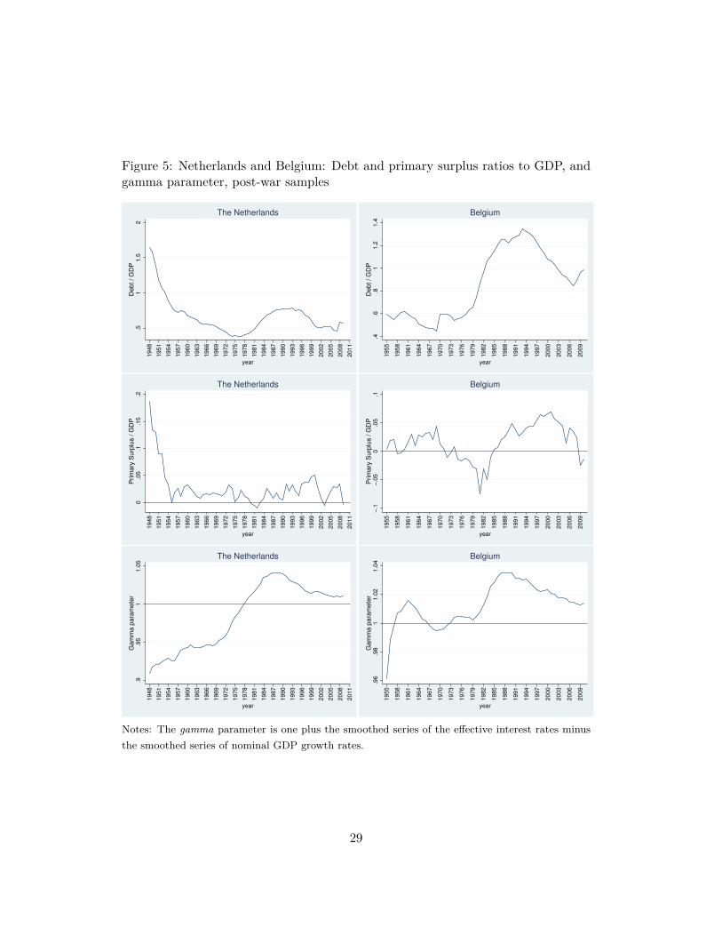
Figure 5: Netherlands and Belgium: Debt and primary surplus ratios to GDP, andgamma parameter, post-war samples

.51

1.5

2D

eb

t /

GD

P

1948

1951

1954

1957

1960

1963

1966

1969

1972

1975

1978

1981

1984

1987

1990

1993

1996

1999

2002

2005

2008

2011

year

The Netherlands

.4.6

.81

1.2

1.4

De

bt

/ G

DP

1955

1958

1961

1964

1967

1970

1973

1976

1979

1982

1985

1988

1991

1994

1997

2000

2003

2006

2009

year

Belgium

0.0

5.1

.15

.2P

rim

ary

Su

rplu

s /

GD

P

1948

1951

1954

1957

1960

1963

1966

1969

1972

1975

1978

1981

1984

1987

1990

1993

1996

1999

2002

2005

2008

2011

year

The Netherlands−

.1−

.05

0.0

5.1

Prim

ary

Su

rplu

s /

GD

P

1955

1958

1961

1964

1967

1970

1973

1976

1979

1982

1985

1988

1991

1994

1997

2000

2003

2006

2009

year

Belgium

.9.9

51

1.0

5G

am

ma

pa

ram

ete

r

1948

1951

1954

1957

1960

1963

1966

1969

1972

1975

1978

1981

1984

1987

1990

1993

1996

1999

2002

2005

2008

2011

year

The Netherlands

.96

.98

11.0

21.0

4G

am

ma

pa

ram

ete

r

1955

1958

1961

1964

1967

1970

1973

1976

1979

1982

1985

1988

1991

1994

1997

2000

2003

2006

2009

year

Belgium

Notes: The gamma parameter is one plus the smoothed series of the effective interest rates minusthe smoothed series of nominal GDP growth rates.

29

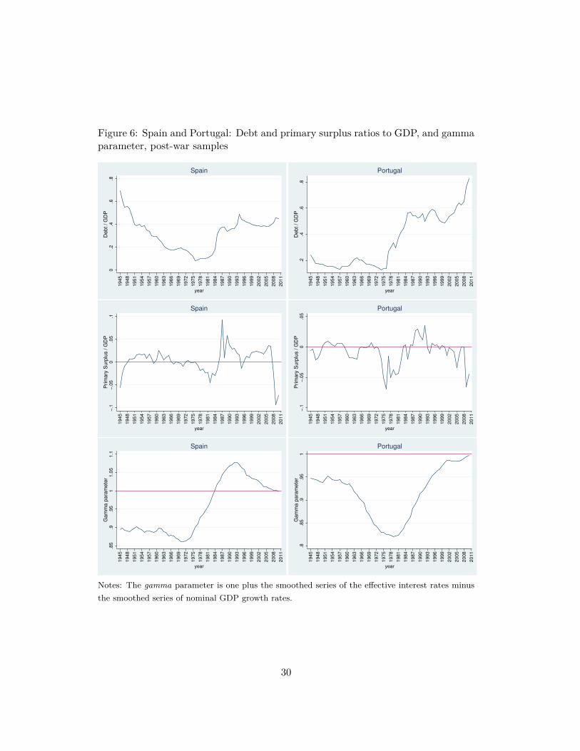
Figure 6: Spain and Portugal: Debt and primary surplus ratios to GDP, and gammaparameter, post-war samples

0.2

.4.6

.8D

eb

t /

GD

P

1945

1948

1951

1954

1957

1960

1963

1966

1969

1972

1975

1978

1981

1984

1987

1990

1993

1996

1999

2002

2005

2008

2011

year

Spain

.2.4

.6.8

Deb

t /

GD

P

1945

1948

1951

1954

1957

1960

1963

1966

1969

1972

1975

1978

1981

1984

1987

1990

1993

1996

1999

2002

2005

2008

2011

year

Portugal

−.1

−.0

50

.05

.1P

rim

ary

Su

rplu

s /

GD

P

1945

1948

1951

1954

1957

1960

1963

1966

1969

1972

1975

1978

1981

1984

1987

1990

1993

1996

1999

2002

2005

2008

2011

year

Spain−

.1−

.05

0.0

5P

rim

ary

Su

rplu

s /

GD

P

1945

1948

1951

1954

1957

1960

1963

1966

1969

1972

1975

1978

1981

1984

1987

1990

1993

1996

1999

2002

2005

2008

2011

year

Portugal

.85

.9.9

51

1.0

51.1

Ga

mm

a p

ara

me

ter

1945

1948

1951

1954

1957

1960

1963

1966

1969

1972

1975

1978

1981

1984

1987

1990

1993

1996

1999

2002

2005

2008

2011

year

Spain

.8.8

5.9

.95

1G

am

ma

pa

ram

ete

r

1945

1948

1951

1954

1957

1960

1963

1966

1969

1972

1975

1978

1981

1984

1987

1990

1993

1996

1999

2002

2005

2008

2011

year

Portugal

Notes: The gamma parameter is one plus the smoothed series of the effective interest rates minusthe smoothed series of nominal GDP growth rates.

30

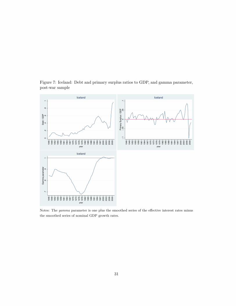
Figure 7: Iceland: Debt and primary surplus ratios to GDP, and gamma parameter,post-war sample

0.2

.4.6

.81

Deb

t /

GD

P

1946

1949

1952

1955

1958

1961

1964

1967

1970

1973

1976

1979

1982

1985

1988

1991

1994

1997

2000

2003

2006

2009

year

Iceland

−.1

−.0

50

.05

.1P

rim

ary

Su

rplu

s /

GD

P

1946

1949

1952

1955

1958

1961

1964

1967

1970

1973

1976

1979

1982

1985

1988

1991

1994

1997

2000

2003

2006

2009

year

Iceland

.7.8

.91

Gam

ma

para

me

ter

1946

1949

1952

1955

1958

1961

1964

1967

1970

1973

1976

1979

1982

1985

1988

1991

1994

1997

2000

2003

2006

2009

year

Iceland

Notes: The gamma parameter is one plus the smoothed series of the effective interest rates minusthe smoothed series of nominal GDP growth rates.

31

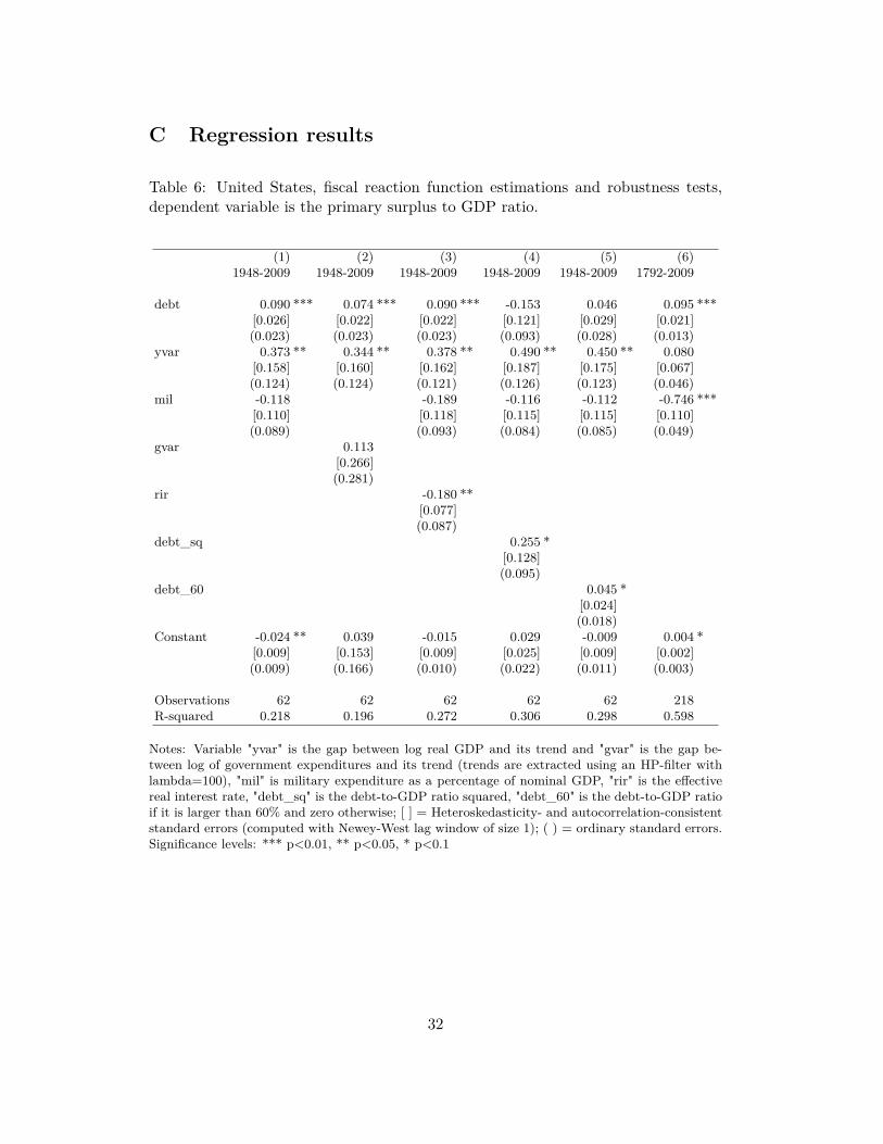
C Regression results

Table 6: United States, fiscal reaction function estimations and robustness tests,dependent variable is the primary surplus to GDP ratio.

(1) (2) (3) (4) (5) (6)1948-2009 1948-2009 1948-2009 1948-2009 1948-2009 1792-2009

debt 0.090 *** 0.074 *** 0.090 *** -0.153 0.046 0.095 ***[0.026] [0.022] [0.022] [0.121] [0.029] [0.021](0.023) (0.023) (0.023) (0.093) (0.028) (0.013)

yvar 0.373 ** 0.344 ** 0.378 ** 0.490 ** 0.450 ** 0.080[0.158] [0.160] [0.162] [0.187] [0.175] [0.067](0.124) (0.124) (0.121) (0.126) (0.123) (0.046)

mil -0.118 -0.189 -0.116 -0.112 -0.746 ***[0.110] [0.118] [0.115] [0.115] [0.110](0.089) (0.093) (0.084) (0.085) (0.049)

gvar 0.113[0.266](0.281)

rir -0.180 **[0.077](0.087)

debt_sq 0.255 *[0.128](0.095)

debt_60 0.045 *[0.024](0.018)

Constant -0.024 ** 0.039 -0.015 0.029 -0.009 0.004 *[0.009] [0.153] [0.009] [0.025] [0.009] [0.002](0.009) (0.166) (0.010) (0.022) (0.011) (0.003)

Observations 62 62 62 62 62 218R-squared 0.218 0.196 0.272 0.306 0.298 0.598

Notes: Variable "yvar" is the gap between log real GDP and its trend and "gvar" is the gap be-tween log of government expenditures and its trend (trends are extracted using an HP-filter withlambda=100), "mil" is military expenditure as a percentage of nominal GDP, "rir" is the effectivereal interest rate, "debt_sq" is the debt-to-GDP ratio squared, "debt_60" is the debt-to-GDP ratioif it is larger than 60% and zero otherwise; [ ] = Heteroskedasticity- and autocorrelation-consistentstandard errors (computed with Newey-West lag window of size 1); ( ) = ordinary standard errors.Significance levels: *** p<0.01, ** p<0.05, * p<0.1

32

Table 7: United Kingdom, fiscal reaction function estimations and robustness tests,dependent variable is the primary surplus to GDP ratio.

(1) (2) (3) (4) (5) (6)1946-2009 1946-2009 1946-2009 1946-2009 1946-2009 1691-2009

debt 0.045 *** 0.019 ** 0.048 *** 0.026 0.052 0.048 ***[0.009] [0.008] [0.009] [0.026] [0.036] [0.002](0.007) (0.007) (0.008) (0.026) (0.029) (0.002)

yvar 0.258 0.218 0.278 0.290 0.261 -0.251 **[0.203] [0.196] [0.201] [0.219] [0.206] [0.115](0.136) (0.128) (0.138) (0.142) (0.137) (0.047)

mil -0.209 *** -0.210 *** -0.231 *** -0.212 *** -0.705 ***[0.051] [0.051] [0.053] [0.053] [0.059](0.071) (0.071) (0.077) (0.072) (0.017)

gvar -0.205 ***[0.057](0.049)

rir 0.079[0.099](0.085)

debt_sq 0.009[0.012](0.012)

debt_60 -0.005[0.025](0.020)

Constant -0.004 0.002 -0.008 0.004 -0.006 0.010 ***[0.008] [0.008] [0.008] [0.013] [0.016] [0.003](0.005) (0.005) (0.007) (0.012) (0.012) (0.002)

Observations 64 64 64 64 64 319R-squared 0.417 0.483 0.426 0.423 0.418 0.887

Notes: Variable "yvar" is the gap between log real GDP and its trend and "gvar" is the gap be-tween log of government expenditures and its trend (trends are extracted using an HP-filter withlambda=100), "mil" is military expenditure as a percentage of nominal GDP, "rir" is the real in-terest rate, "debt_sq" is the debt-to-GDP ratio squared, "debt_60" is the debt-to-GDP ratio ifit is larger than 60% and zero otherwise; [ ] = Heteroskedasticity- and autocorrelation-consistentstandard errors (computed with Newey-West lag window of size 1); ( ) = ordinary standard errors.Significance levels: *** p<0.01, ** p<0.05, * p<0.1

33

Table 8: Netherlands, fiscal reaction function estimations and robustness tests, de-pendent variable is the primary surplus to GDP ratio.

(1) (2) (3) (4) (5)1948-2010 1948-2010 1948-2010 1948-2010 1816-2010

debt 0.074 *** 0.076 *** -0.135 * 0.105 *** 0.031 ***[0.013] [0.012] [0.069] [0.027] [0.004](0.011) (0.011) (0.048) (0.029) (0.003)

yvar 0.341 ** 0.282 * 0.196 0.346 ** 0.161[0.148] [0.152] [0.137] [0.145] [0.105](0.101) (0.106) (0.093) (0.101) (0.064)

gvar 0.069 0.064 -0.090 0.043 0.027[0.047] [0.047] [0.061] [0.049] [0.048](0.033) (0.033) (0.046) (0.040) (0.020)

rir -0.095[0.058](0.060)

debt_sq 0.141 ***[0.047](0.031)

debt_60 -0.015[0.012](0.013)

Constant -0.026 *** -0.024 *** 0.046 * -0.039 *** -0.010 *[0.008] [0.007] [0.023] [0.013] [0.005](0.007) (0.007) (0.017) (0.014) (0.004)

Observations 62 62 62 62 186R-squared 0.795 0.804 0.849 0.800 0.379

Notes: Variable "yvar" is the gap between log real GDP and its trend and "gvar" is the gap be-tween log of government expenditures and its trend (trends are extracted using an HP-filter withlambda=100), "rir" is the real interest rate, "debt_sq" is the debt-to-GDP ratio squared, "debt_60"is the debt-to-GDP ratio if it is larger than 60% and zero otherwise; [ ] = Heteroskedasticity- andautocorrelation-consistent standard errors (computed with Newey-West lag window of size 1); ( )= ordinary standard errors. Significance levels: *** p<0.01, ** p<0.05, * p<0.1

34

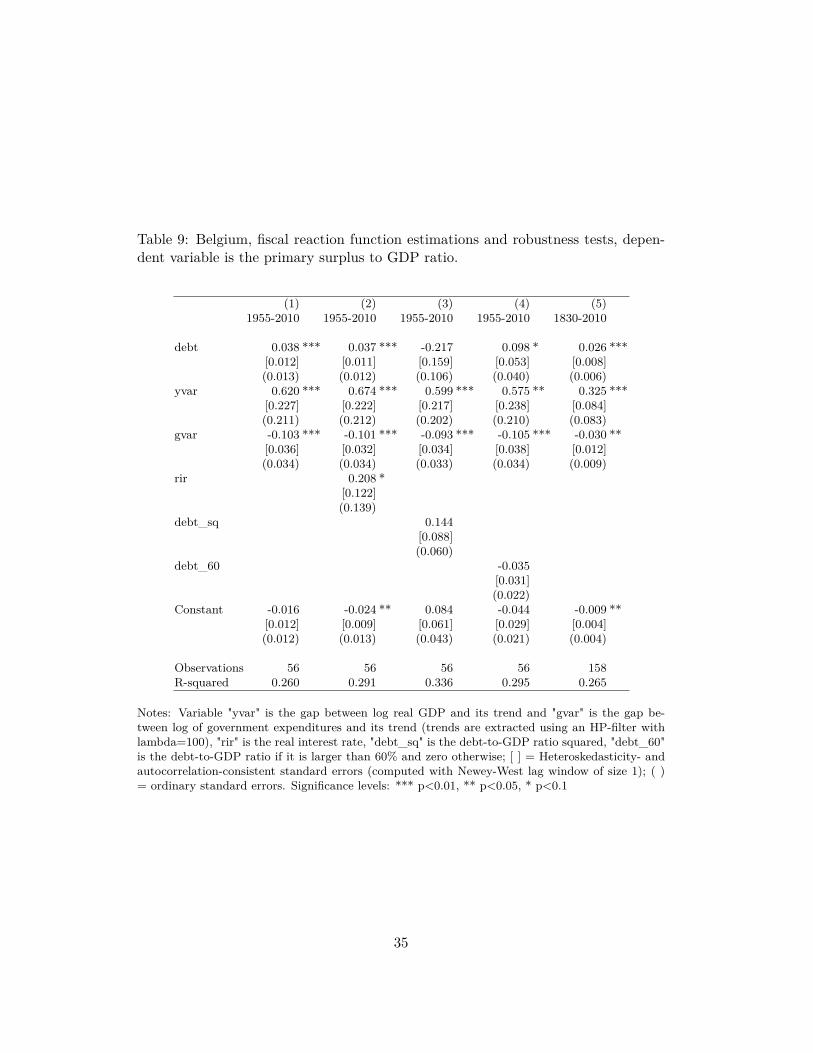
Table 9: Belgium, fiscal reaction function estimations and robustness tests, depen-dent variable is the primary surplus to GDP ratio.

(1) (2) (3) (4) (5)1955-2010 1955-2010 1955-2010 1955-2010 1830-2010

debt 0.038 *** 0.037 *** -0.217 0.098 * 0.026 ***[0.012] [0.011] [0.159] [0.053] [0.008](0.013) (0.012) (0.106) (0.040) (0.006)

yvar 0.620 *** 0.674 *** 0.599 *** 0.575 ** 0.325 ***[0.227] [0.222] [0.217] [0.238] [0.084](0.211) (0.212) (0.202) (0.210) (0.083)

gvar -0.103 *** -0.101 *** -0.093 *** -0.105 *** -0.030 **[0.036] [0.032] [0.034] [0.038] [0.012](0.034) (0.034) (0.033) (0.034) (0.009)

rir 0.208 *[0.122](0.139)

debt_sq 0.144[0.088](0.060)

debt_60 -0.035[0.031](0.022)

Constant -0.016 -0.024 ** 0.084 -0.044 -0.009 **[0.012] [0.009] [0.061] [0.029] [0.004](0.012) (0.013) (0.043) (0.021) (0.004)

Observations 56 56 56 56 158R-squared 0.260 0.291 0.336 0.295 0.265

Notes: Variable "yvar" is the gap between log real GDP and its trend and "gvar" is the gap be-tween log of government expenditures and its trend (trends are extracted using an HP-filter withlambda=100), "rir" is the real interest rate, "debt_sq" is the debt-to-GDP ratio squared, "debt_60"is the debt-to-GDP ratio if it is larger than 60% and zero otherwise; [ ] = Heteroskedasticity- andautocorrelation-consistent standard errors (computed with Newey-West lag window of size 1); ( )= ordinary standard errors. Significance levels: *** p<0.01, ** p<0.05, * p<0.1

35

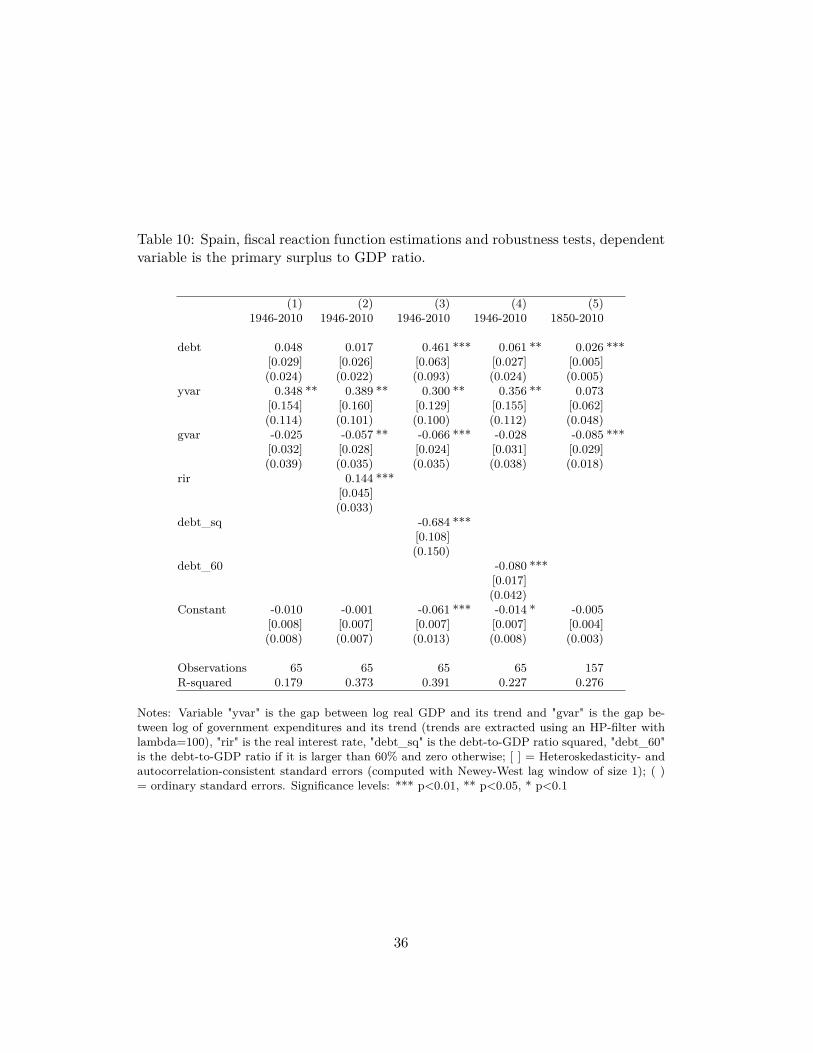
Table 10: Spain, fiscal reaction function estimations and robustness tests, dependentvariable is the primary surplus to GDP ratio.

(1) (2) (3) (4) (5)1946-2010 1946-2010 1946-2010 1946-2010 1850-2010

debt 0.048 0.017 0.461 *** 0.061 ** 0.026 ***[0.029] [0.026] [0.063] [0.027] [0.005](0.024) (0.022) (0.093) (0.024) (0.005)

yvar 0.348 ** 0.389 ** 0.300 ** 0.356 ** 0.073[0.154] [0.160] [0.129] [0.155] [0.062](0.114) (0.101) (0.100) (0.112) (0.048)

gvar -0.025 -0.057 ** -0.066 *** -0.028 -0.085 ***[0.032] [0.028] [0.024] [0.031] [0.029](0.039) (0.035) (0.035) (0.038) (0.018)

rir 0.144 ***[0.045](0.033)

debt_sq -0.684 ***[0.108](0.150)

debt_60 -0.080 ***[0.017](0.042)

Constant -0.010 -0.001 -0.061 *** -0.014 * -0.005[0.008] [0.007] [0.007] [0.007] [0.004](0.008) (0.007) (0.013) (0.008) (0.003)

Observations 65 65 65 65 157R-squared 0.179 0.373 0.391 0.227 0.276

Notes: Variable "yvar" is the gap between log real GDP and its trend and "gvar" is the gap be-tween log of government expenditures and its trend (trends are extracted using an HP-filter withlambda=100), "rir" is the real interest rate, "debt_sq" is the debt-to-GDP ratio squared, "debt_60"is the debt-to-GDP ratio if it is larger than 60% and zero otherwise; [ ] = Heteroskedasticity- andautocorrelation-consistent standard errors (computed with Newey-West lag window of size 1); ( )= ordinary standard errors. Significance levels: *** p<0.01, ** p<0.05, * p<0.1

36

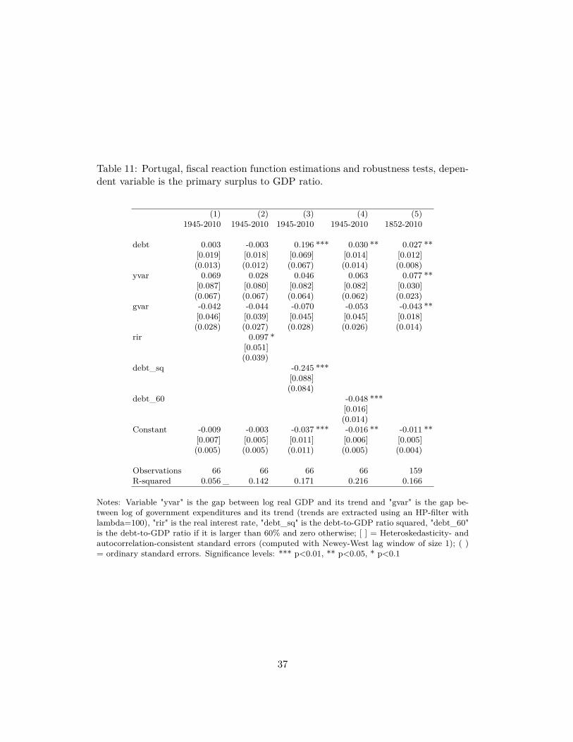
Table 11: Portugal, fiscal reaction function estimations and robustness tests, depen-dent variable is the primary surplus to GDP ratio.

(1) (2) (3) (4) (5)1945-2010 1945-2010 1945-2010 1945-2010 1852-2010

debt 0.003 -0.003 0.196 *** 0.030 ** 0.027 **[0.019] [0.018] [0.069] [0.014] [0.012](0.013) (0.012) (0.067) (0.014) (0.008)

yvar 0.069 0.028 0.046 0.063 0.077 **[0.087] [0.080] [0.082] [0.082] [0.030](0.067) (0.067) (0.064) (0.062) (0.023)

gvar -0.042 -0.044 -0.070 -0.053 -0.043 **[0.046] [0.039] [0.045] [0.045] [0.018](0.028) (0.027) (0.028) (0.026) (0.014)

rir 0.097 *[0.051](0.039)

debt_sq -0.245 ***[0.088](0.084)

debt_60 -0.048 ***[0.016](0.014)

Constant -0.009 -0.003 -0.037 *** -0.016 ** -0.011 **[0.007] [0.005] [0.011] [0.006] [0.005](0.005) (0.005) (0.011) (0.005) (0.004)

Observations 66 66 66 66 159R-squared 0.056 _ 0.142 0.171 0.216 0.166

Notes: Variable "yvar" is the gap between log real GDP and its trend and "gvar" is the gap be-tween log of government expenditures and its trend (trends are extracted using an HP-filter withlambda=100), "rir" is the real interest rate, "debt_sq" is the debt-to-GDP ratio squared, "debt_60"is the debt-to-GDP ratio if it is larger than 60% and zero otherwise; [ ] = Heteroskedasticity- andautocorrelation-consistent standard errors (computed with Newey-West lag window of size 1); ( )= ordinary standard errors. Significance levels: *** p<0.01, ** p<0.05, * p<0.1

37

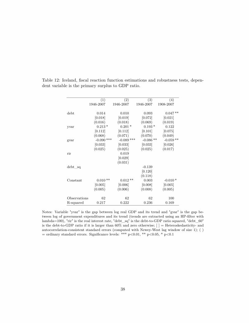
Table 12: Iceland, fiscal reaction function estimations and robustness tests, depen-dent variable is the primary surplus to GDP ratio.

(1) (2) (3) (4)1946-2007 1946-2007 1946-2007 1908-2007

debt 0.014 0.010 0.093 0.047 **[0.018] [0.019] [0.072] [0.021](0.016) (0.018) (0.069) (0.019)

yvar 0.213 * 0.201 * 0.193 * 0.122[0.112] [0.112] [0.101] [0.075](0.068) (0.071) (0.070) (0.049)

gvar -0.090 *** -0.089 *** -0.086 ** -0.059 **[0.033] [0.033] [0.033] [0.026](0.025) (0.025) (0.025) (0.017)

rir 0.019[0.029](0.031)

debt_sq -0.139[0.120](0.118)

Constant 0.010 ** 0.012 ** 0.003 -0.010 *[0.005] [0.006] [0.008] [0.005](0.005) (0.006) (0.008) (0.005)

Observations 62 62 62 100R-squared 0.217 0.222 0.236 0.169

Notes: Variable "yvar" is the gap between log real GDP and its trend and "gvar" is the gap be-tween log of government expenditures and its trend (trends are extracted using an HP-filter withlambda=100), "rir" is the real interest rate, "debt_sq" is the debt-to-GDP ratio squared, "debt_60"is the debt-to-GDP ratio if it is larger than 60% and zero otherwise; [ ] = Heteroskedasticity- andautocorrelation-consistent standard errors (computed with Newey-West lag window of size 1); ( )= ordinary standard errors. Significance levels: *** p<0.01, ** p<0.05, * p<0.1

38

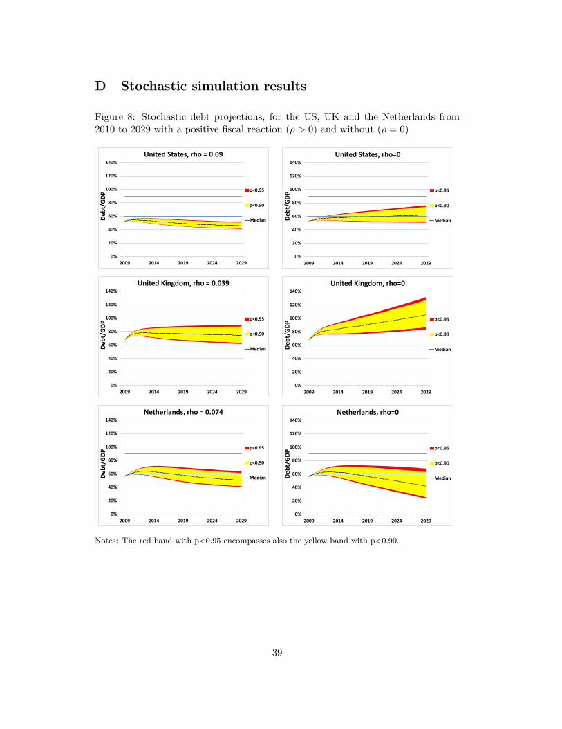
D Stochastic simulation results

Figure 8: Stochastic debt projections, for the US, UK and the Netherlands from2010 to 2029 with a positive fiscal reaction (𝜌 > 0) and without (𝜌 = 0)

0%

20%

40%

60%

80%

100%

120%

140%

2009 2014 2019 2024 2029

De

bt/

GD

P

United States, rho = 0.09

p<0.95

p<0.90

Median

0%

20%

40%

60%

80%

100%

120%

140%

2009 2014 2019 2024 2029

De

bt/

GD

P

United States, rho=0

p<0.95

p<0.90

Median

0%

20%

40%

60%

80%

100%

120%

140%

2009 2014 2019 2024 2029

De

bt/

GD

P

United Kingdom, rho = 0.039

p<0.95

p<0.90

Median

0%

20%

40%

60%

80%

100%

120%

140%

2009 2014 2019 2024 2029

De

bt/

GD

P

United Kingdom, rho=0

p<0.95

p<0.90

Median

0%

20%

40%

60%

80%

100%

120%

140%

2009 2014 2019 2024 2029

De

bt/

GD

P

Netherlands, rho = 0.074

p<0.95

p<0.90

Median

0%

20%

40%

60%

80%

100%

120%

140%

2009 2014 2019 2024 2029

De

bt/

GD

P

Netherlands, rho=0

p<0.95

p<0.90

Median

Notes: The red band with p<0.95 encompasses also the yellow band with p<0.90.

39

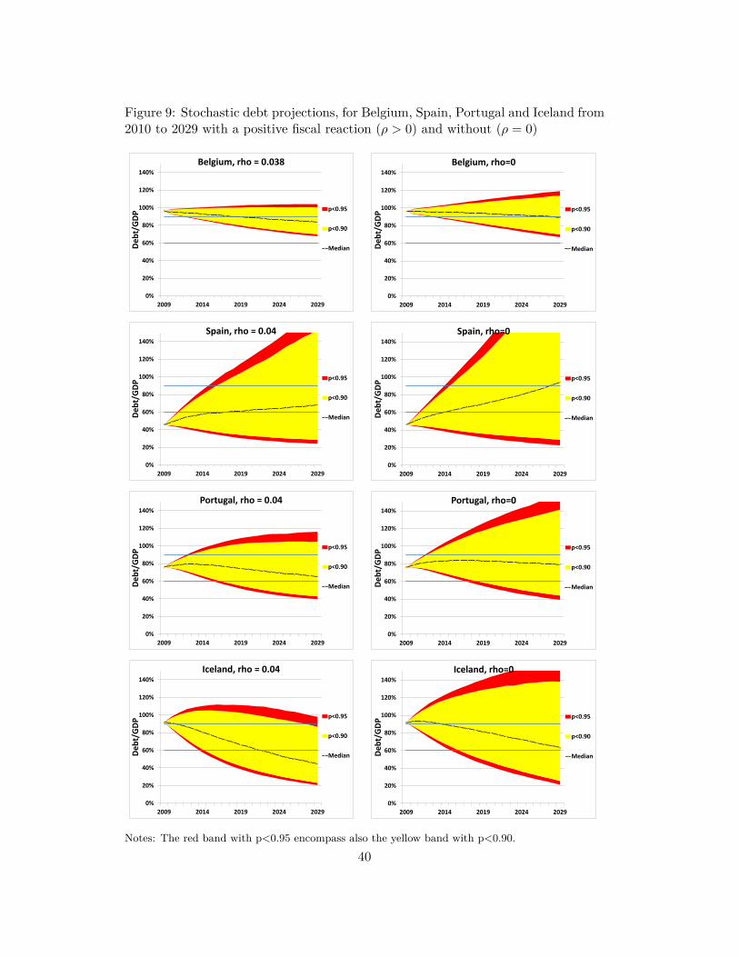
Figure 9: Stochastic debt projections, for Belgium, Spain, Portugal and Iceland from2010 to 2029 with a positive fiscal reaction (𝜌 > 0) and without (𝜌 = 0)

0%

20%

40%

60%

80%

100%

120%

140%

2009 2014 2019 2024 2029

De

bt/

GD

P

Belgium, rho = 0.038

p<0.95

p<0.90

Median

0%

20%

40%

60%

80%

100%

120%

140%

2009 2014 2019 2024 2029

De

bt/

GD

P

Belgium, rho=0

p<0.95

p<0.90

Median

0%

20%

40%

60%

80%

100%

120%

140%

2009 2014 2019 2024 2029

De

bt/

GD

P

Spain, rho = 0.04

p<0.95

p<0.90

Median

0%

20%

40%

60%

80%

100%

120%

140%

2009 2014 2019 2024 2029

De

bt/

GD

P

Spain, rho=0

p<0.95

p<0.90

Median

0%

20%

40%

60%

80%

100%

120%

140%

2009 2014 2019 2024 2029

De

bt/

GD

P

Portugal, rho = 0.04

p<0.95

p<0.90

Median

0%

20%

40%

60%

80%

100%

120%

140%

2009 2014 2019 2024 2029

De

bt/

GD

P

Portugal, rho=0

p<0.95

p<0.90

Median

0%

20%

40%

60%

80%

100%

120%

140%

2009 2014 2019 2024 2029

De

bt/

GD

P

Iceland, rho = 0.04

p<0.95

p<0.90

Median

0%

20%

40%

60%

80%

100%

120%

140%

2009 2014 2019 2024 2029

De

bt/

GD

P

Iceland, rho=0

p<0.95

p<0.90

Median

Notes: The red band with p<0.95 encompass also the yellow band with p<0.90.

40

Publisher:

CPB Netherlands Bureau for Economic Policy AnalysisP.O. Box 80510 | 2508 GM The Haguet (070) 3383 380

June 2012 | ISBN 978-90-5833-554-8