When the Levee Breaks:

Labor Mobility and Economic Development

in the American South∗

Richard Hornbeck

Harvard University and NBER

Suresh Naidu

Columbia University and NBER

January 2012

Abstract

The availability of low-wage immobile labor may discourage economic development.

In the American South, post-bellum economic stagnation has been partially attributed

to white landowners’ access to immobile low-wage black workers; indeed, subsequent

Southern economic convergence was associated with substantial black out-migration.

This paper estimates that the 1927 Mississippi flood caused immediate and persis-

tent out-migration of black workers from flooded counties. Following this decline in

the availability of low-wage black labor, landowners in flooded counties dramatically

mechanized and modernized agricultural production relative to landowners in nearby

similar non-flooded counties. The temporary displacement of black workers led to a

permanent economic transition, though landowners had incentives to discourage black

out-migration and maintain a system of labor-intensive agricultural production.

JEL: N52, N32, O10

∗For comments and suggestions, we thank seminar participants at Columbia, Pittsburgh, and Harvard.For financial support, we thank the WCFIA’s Project on Justice, Welfare, and Economics. Tom Beck-ford, James Feigenbaum, Lillian Fine, Andrew Das Sarma, and Leo Schwartz provided excellent researchassistance.

Under-developed societies often contain a large population of immobile low-wage agri-

cultural workers, despite having the potential physical, technological, and human resources

for widespread economic growth. The classic Lewis (1954) model of underdevelopment had

informal institutions keeping an inefficiently high number of workers in the rural sector. In

the rare “growth miracle,” increased capital investment and technological improvement leads

to economic development. Among the factors that constrain such economic development, a

large low-wage population may discourage technological innovation (Habakkuk, 1962; Allen,

2009) or indirectly encourage exploitative institutions that limit economic growth (Acemoglu,

Johnson and Robinson, 2002; Engerman and Sokoloff, 2012). Conversely, migration and gen-

eral labor market mobility may encourage structural economic development (Kuznets, 1955;

Banerjee and Newman, 1998).

The Southern United States experienced a remarkable economic transition from 1940 to

1970, as documented in Gavin Wright’s “Old South, New South” (Wright, 1986). The US

South changed from a largely agrarian low-wage economy to a more industrial economy pay-

ing comparable wages to the North; within the agricultural sector, production became more

capital-intensive and farm sizes increased. Southern economic modernization and agricul-

tural mechanization coincided with large-scale black out-migration, though a direct causal

relationship is difficult to observe.

At the beginning of the 20th century, despite political integration with the North, the

South remained undemocratic and white planters dominated areas with concentrated black

populations. The Mississippi Delta, with its small wealthy white planter minority and large

number of poor black workers, exemplified the racial inequality and discrimination that

fostered paternalistic black labor relations and restricted black labor mobility.

This paper examines the relationship between black out-migration and Southern eco-

nomic transition, as reflected in the impacts of the Great Mississippi Flood of 1927. The

Great Flood of 1927 displaced at least 325,000 people and disrupted the traditional racial

labor market equilibrium, leading to a large exodus of black laborers and sharecroppers

from flooded areas. Over time, following this decline in black labor abundance, agriculture

in flooded counties became substantially mechanized and modernized in flooded counties

relative to nearby similar non-flooded counties. Landowners resisted black out-migration,

consistent with estimated changes in agricultural land values. The persistence of Southern

labor-intensive agricultural production was sustained, in part, by the presence of a large

immobile black agricultural labor force.

Using county-level data from the Census of Agriculture and Population, from 1900 to

1970, the main empirical specifications compare changes between flooded counties and non-

flooded counties within the same state and with similar pre-1927 outcome values. The empir-

1

ical estimates are robust to controlling for other differences between flooded and non-flooded

counties, including differential changes associated with: distance to the Mississippi river;

geographic suitability for cotton and corn; terrain ruggedness; or longitude and latitude.

Across the various outcome variables, interpretation of the results appears less consistent

with direct impacts of the flood on capital reconstruction or land productivity. Further,

general equilibirum impacts on non-flooded counties appear to be small.

In the wake of the 1927 flood, black out-migration and the modernization of agricul-

ture in flooded areas provides a microcosm of subsequent black out-migration and economic

development across the American South. In under-developed societies with substantial pop-

ulations of immobile low-wage agricultural laborers, an increase in labor mobility and rural

out-migration may generate a sustained economic transition toward increased agricultural

mechanization and modernization. Whether caused by “push factors,” such as rural natural

disasters, or caused by “pull factors,” such as urban labor demand, decreased agricultural

labor surpluses may promote structural economic development.

Section I provides historical background on the Southern economy and the Mississippi

Delta, and reviews contemporary qualitative accounts on the impact of the 1927 flood.

Section II outlines a simple model of labor mobility and economic transition, reflecting

historical accounts and motiviating the empirical estimates. Section III presents the data

and explores initial differences in flooded and non-flooded counties. Section IV describes the

empirical methodology. Section V reports the baseline results, examines their robustness,

and discusses potential alternative interpretations. Section VI concludes.

I Historical Background

I.A Southern Underdevelopment and The Mississippi Delta

Even prior to the revolutionary war, the Southern economy was distinctive. Slavery and a

geographic suitability for plantation agriculture contributed to a system of labor-intensive

agricultural production. As slavery expanded into new states during the 19th century, po-

litical conflict between Northern free states and Southern slave states culiminated in the

Civil War. Four million slaves were emancipated and enfranchised; by 1900, however, most

Southern states had effectively disenfranchised black populations via poll taxes and literacy

tests (Naidu, 2011).

White Southern planters used their political influence to restrict black labor mobility

and exert control over black agricultural workers.1 Anti-enticement laws made it illegal

for one planter to hire another planter’s workers, while anti-vagrancy laws made it illegal

1Agricultural “workers” include both wage laborers and tenant farmers, who received “wages” in the formof production shares, housing, and advances of equipment and/or money.

2

to be unemployed and without housing. Due to such labor laws, the underprovision of

schools, and local credit market monopolies, black workers were constrained in their ability

to choose locations and employers (Mandle, 1978; Margo, 1994; Ransom and Sutch, 2001;

Naidu, 2010). Southern planters valued black labor immensely, and made every attempt to

restrict labor mobility.2 Gunnar Myrdal summarized this system of labor control, writing

that “Southerners still think of their Negroes as former slaves” (Myrdal, 1944).

The threat of racial violence underlay Southern labor relations (Rosengarten, 1975; Tol-

nay and Beck, 1995). Southern planters often pursued a strategy of paternalism to retain

labor, offering protection from white violence and implicit insurance. “Protection was impor-

tant .... particularly for black workers, because they lacked civil rights and society condoned

violence”(Alston and Ferrie, 1999, p. 20). During a period of labor scarcity, a team of anthro-

pologists observed: “One of the bases of competition between landlords for tenants was the

landlord’s reputation among tenants with regard to his use of physical violence. At the same

time the field evidence reveals that the use of threats of violence by white planters is one

of the basic controls upon labor” (Davis, Gardner and Gardner, 2009, p. 392). Rather than

generating a large flight of black labor, the constant threat of violence induced a demand for

white protection and kept black workers tied to particular employers.

The Southern economy remained persistently under-developed between the Civil War and

World War II, despite economic and political integration with the Northern United States.

While the North developed large manufacturing sectors, the South remained primarily agri-

cultural. Northern wheat threshing became increasingly mechanized in the 19th century

(David, 1975), while Southern cotton harvesting mechanization was delayed until the mid-

20th century (Fleisig, 1965; Whatley, 1987). In cotton farming, “technology for mechanizing

the preharvest operations was available well before the 1930s, yet it was hardly used at all

in the South, and least of all in the plantation belt” (Wright, 1986, p. 133). Early cotton

mechanization entailed replacing mule- and horse-drawn plows and tillers with tractor-drawn

tillers, and was associated with a 30% reduction in labor inputs (Hurst, 1933).3 The relative

abundance of low-wage immobile black labor is one proposed explanation for the delayed

economic development of the American South (Whatley, 1987).

Southern economic modernization and agricultural mechanization coincided with large-

scale black out-migration. Wright (1986) describes a 1940 to 1970 economic transition from

the “Old South” to the “New South,” attributing much of this change to a breakdown

of segmented labor markets and increased mobility of Southern blacks. Contemporaries

2Widespread racial discrimination also contributed to reduced labor market mobility of black Americans.3Early tractors also transported picked cotton from the fields to gins, replacing slow and inefficient mule-

drawn carts (Ellenberg, 2007).

3

recognized a dual relationship between labor scarcity encouraging agricultural mechanization

and technological improvements displacing workers (Raper, 1946). Farm sizes increased

as agriculture became more capital-intensive and as mules and horses were replaced with

tractors and harvesters (Kirby, 1987).

The United States’ Southern economy experienced a 20th century growth miracle. Much

of the regional convergence in the United States is driven by labor movement out of South-

ern agriculture and relative increases in Southern agricultural wages (Caselli and Coleman,

2001). Aside from the role of black out-migration, additional important events were the New

Deal, World War II, and Civil Rights regulation (Wright, 1986; Heckman and Payner, 1989;

Donohue and Heckman, 1991; Besley, Persson and Sturm, 2010).4

The lower Mississippi region, particularly the Mississippi-Yazoo Delta, embodied histor-

ical Southern underdevelopment. The Delta has been dubbed the “most southern place

on earth” (Cobb, 1994), and became infamous for racial inequality and abuse.5 However,

powerful white planters recognized their economic dependence on local black labor. White

planters experimented with recruiting Chinese and Italian workers, but were unable to find

adequate and willing substitutes. Local elites, such as Leroy Percy, extended credit to blacks

and resisted the Klu Klux Klan to retain a local labor force, a task that became difficult as

World War I and the first Great Migration cracked the walls keeping black labor isolated.

Nonetheless, over the 20th century, the Delta would experience an exodus of black labor and

agricultural modernization.

I.B The Great Mississippi Flood of 1927

“A great deal of labor from the flooded section after being returned to the plan-

tations is going North. It is thus a serious menace and it is going to offer a

tremendous problem to all of us” – Alex Scott, Delta planter.

The Mississippi river basin is massive, stretching into the central United States to channel

water through the slow and winding Mississippi river. The river itself is somewhat undefined,

historically changing course and spilling into natural floodplains. Over the late 19th and early

20th centuries, levees were constructed to contain the river and its natural spillways were

closed off. In 1926, the new chief of the Army Corps of Engineers “for the first time officially

stated in his annual report that the levees were finally in condition ‘to prevent the destructive

effect of floods”’ (Barry, 1998; United States Army Corps of Engineers, 1926, p. 175).

4Additional important factors include disease eradication (Bleakley, 2007) and the introduction of airconditioning (Arsenault, 1984).

5In 1921, William Pickens, Arkansan NAACP secretary, dubbed the Mississippi River Valley the “Amer-ican Congo.” In 1919 alone, at least 18 black citizens were lynched in the Delta (Woodruff, 2003).

4

In 1927, the levee system failed catastrophically along the lower Mississippi river. Heavy

rains throughout the Mississippi river basin accumulated in rising river levels whose enormous

pressure created 145 levee breaks and flooded 26,000 square miles. The flood displaced at

least 325,000 people, and is estimated to have caused $400 million in property damage and

directly killed 246 people (American National Red Cross, 1929; Barry, 1998; Daniel, 1996).

The Red Cross established refugee camps for 325,000 people, though camp administra-

tion was placed under the control of local county governments. Camps were dominated by

white planters and became centers of repression and racial abuse. Black work gangs were

conscripted and forced to work on levees, domestic services, or post-flood planting and har-

vesting of crops. A black insurance officer who refused to work was shot and killed by the

mayor of Lake Providence, LA. One infamous camp in the Delta was controlled by William

Percy, son of LeRoy Percy. William Percy forced blacks to work in the camp for free, wearing

laborer tags to receive food, and any caught attempting to leave were whipped.6

The 1927 flood and its aftermath captured national attention. A circulated black news-

paper, The Chicago Defender, provided detailed accounts of racial abuse in Red Cross relief

camps and listed job openings for blacks in Northern cities.7 A Federal Flood Reconstruc-

tion Bill refused direct relief to individuals, instead providing in-kind transfers through Red

Cross camps.8 Much of the flood aid was captured and redirected by white elites, and often

withheld unless blacks worked on the levees or planters’ farms.

Faced with the potential exodus of black workers, white planters made every effort to

retain their black labor force (Spencer, 1994). Following directives from the Mississippi

governer and the National Guard commander, the Red Cross issued a memo on the “return

of refugees,” stating: “Plantation owners desiring their labor to be returned from Refugee

Camps will make application to the nearest Red Cross representative,” whereupon they “will

issue passes to refugees” (Barry, 1998, pp. 313-314). The Delta & Pine Land Company, the

nation’s largest cotton plantation, established its own refugee camp and had its workers

transferred by special train.

Despite such efforts, or even perhaps encouraged by such efforts, many black families left

6(Barry, 1998, p. 315) recorded a black man saying: “The colored people caught tough times aroundGreenville.... Whites were kicking coloreds and beating them and knocking them around like dogs. Hungrypeople, they wouldn’t feed them sometimes.” A white woman remembered: “The [National] Guard wouldcome along and say ‘There’s a boat coming up. Go unload.’ If they didn’t hurry up, they’d kick them. Theydidn’t mind taking their guns, pistols our, and knocking them over the head.”

7Commerce Secretary Herbert Hoover gained national prominence through his management of flood reliefoperations and secured the presidential nomination. However, racial abuses during the flood eventually costhim the support of national black leader Robert Moton, who had been in charge of investigating racial abusesin relief camps, and contributed to the departure of blacks from the Republican party.

8The Bill prefigured New Deal legislation by providing a federal transfer to landowners without requiringlocal contributions.

5

flooded counties in search of better political and economic opportunities. Contemporaneous

accounts describe black families, once displaced from their homes, continuing on to Chicago

and other Northern cities.9 After such harrowing racial abuses, white planters in flooded

areas retained little credibility in offering paternalistic protection to their black workers.

Social networks shifted toward favoring migration; in Greenville MS, black leaders left for

Chicago and crowds of blacks gathered at the local railway station every Saturday night to

see who was leaving and say goodbye (Barry, 1998, p. 416). The director of the Delta Land

and Pine Company reported to shareholders: “Labor was completely demoralized and the

plantation was left almost completeley without labor.” LeRoy Percy reported: “The most

serious thing that confronts the planter in the overflowed territory is the loss of labor, which

is great and is continuing.”

White planters in flooded counties were forced to adapt to the decreased availability of

black workers. In November 1927, the Engineering News Record noted: “In certain sections

of the lower Delta above the Arkansas and Yazoo where are a crop could not be made this year

two-thirds to four-fifths of the families have moved away. In these districts farm-machinery

salesmen have been busy, and farm experts are watching the result with some apprehension.”

In 1931, a Mississippi Agricultural Extension Service bulletin discusses the “serious problem”

of black out-migration and explores “the possible solution in mechanical farming,” comparing

five tenant-operated plantations and five tractor-operated plantations in the Delta (Vaiden,

Smith and Ayres, 1931). Contemporaneous accounts describe a reorganization of agricultural

production and increased mechanization in the Delta: “Many planters have turned to the

use of wage labor and large-scale machinery in an effort to improve production efficiency and

decrease costs.” (Langston and Thibodeaux, 1939, p. 3).

The Mississippi Delta has often been examined as a microcosm of historical Southern

underdevelopment; after the 1927 flood and resulting labor scarcity, the Delta also provides

a microcosm of Southern economic development following black out-migration. In contrast

to the subsequent gradual increase in black mobility across the South, the particular flooded

areas experienced a sharp exogenous increase in black mobility due to temporary displacment,

the destruction of paternalistic institutions, and a shift in black social networks.

II A Model of Economic Transition after Flooding and Labor Displacement

II.A Model Setup

Assume that a representative Southern planter in county c and year t produces agricultural

goods for a world market with fixed prices. The production function is concave in capital

9This episode was influential in the development of Delta blues and Chicago blues (see, e.g., “When theLevee Breaks”).

6

and labor: AcF (Kct, LBct, L

Wct ). Each county has a fixed supply of land with productivity

Ac. Capital Kct is defined broadly to include equipment and machinery, mules and horses,

fertilizer, and land improvements. Capital is sufficiently mobile or depreciable that the

marginal return to capital r is equalized across counties. Labor is supplied inelastically by

resident black workers LBct and resident white workers LW

ct . Capital and labor are substitutes,

reflecting a choice between “Old South” labor-intensive production and “New South” capital-

intensive production.10

Workers are imperfectly mobile and, reflecting historical Southern institutions, black

workers are less mobile than white workers. For analytical simplicitly, assume that white

workers are perfectly mobile and earn a fixed outside “Northern” wage normalized to wW .

Black workers can earn an outside wage wB but must pay a one-time moving cost M equiv-

alent to an annuitized moving cost m; otherwise, black workers earn wB −m in their home

county.

II.B Initial Equilibrium

After the abolition of slavery and initial migration, each county has Lc0 black workers. In the

first period, the Southern planter chooses inputs to maximize: AcF (Kc1, LBc1, L

Wc1 )− rKc1 −

(wB −m)LBc1 − wWLW

c1 , subject to LBc1 ≤ LB

c0. Consistent with efforts by Southern planters

to limit black mobility, assume that the constraint binds and LBc1 = LB

c0. Capital investment

and the number of white workers are determined by:

AcFK(Kc1, LBc0, L

Wc1 ) = r(1)

AcFWL (Kc1, L

Bc0, L

Wc1 ) = wW(2)

In particular, equilibrium choices of capital and white workers depend on the initial number

of black workers: more black workers leads to a lower capital stock and fewer white workers.

II.C Comparative Statics after a Large Flood

Consider the impact of a large flood hitting some counties between periods 1 and 2. The

flood temporarily displaces all workers into refugee camps, temporarily lowering the remain-

ing moving cost of black workers to αM , where α ∈ (0, 1). In practice, the flood may also

encourage migration through other mechanisms: decreased ability of Southern planters to co-

ordinate on restricting black mobility; decreased trust in Southern planters due to widespread

racial abuses; increased information about Northern job opportunities; and changes in black

social networks toward favoring Northern migration.

10Black workers and white workers are also substitutes, though capital-labor substitutability may differbetween black workers and white workers (e.g., due to differences in average education).

7

Northern migration becomes an attractive option to black workers, relative to returning

to lower wages in their home counties. Rather than all black workers migrating North, the

Southern planter may use a combination of incentives and threats to induce workers to return

at cost (1− α)M .

After the flood, the Southern planter chooses inputs to maximize: AcF (Kc2, LBc2, L

Wc2 )−

rKc2 − (wB − αm)LBc2 − wWLW

c2 , subject to LBc2 ≤ LB

c0. The need to compensate and/or

threaten black workers after the flood effectively increases the cost of employing black work-

ers. Assume that the flood’s displacement effect is sufficiently large, i.e., α is sufficiently

small, that the constraint no longer binds and some black workers are allowed to out-migrate

(LBc2 < LB

c0).

Thus, in flooded counties, there is a decline in the number of black workers, an increase in

the capital stock, and an increase in the number of white workers. Intuitively, the loss of low-

wage immobile black workers causes Southern planters to shift toward more capital-intensive

production methods and more white workers. This transition will be especially pronounced

if there is a higher substitutability between capital and black workers; for example, if there

is capital-skill complementarity and white workers are higher-skilled on average.

This stylized model does not include dynamic adjustment costs. In practice, it may take

a number of periods to accumulate the desired capital stock. However, the out-migration of

black workers is predicted to be immediate and persistent.

Agricultural land values decline in this model, reflecting the loss of exploitable low-cost

immobile black labor. For this reason, land-owning Southern planters resist black out-

migration. If there were sufficiently large externalities in capital investment, the flood may

cause a “big push” toward modernization that ultimately increases land values.11 Due to

coordinated investments in new capital equipment and infrastructure, learning-by-doing, or

knowledge spillovers, the private return to capital investment may be increasing in county-

level total capital investment (Romer, 1986; Murphy, Shleifer and Vishny, 1989; Foster and

Rosenzweig, 1995). This class of models predicts that agricultural modernization will increase

over time; for certain parameters only, land values may increase.

11While individual landowners and landowner-collectives resisted out-migration, there may be a long-runcollective interest in landowners encouraging out-migration and modernizing agricultural production. Onelandowner would internalize all such spillover impacts, so it is necessary to consider a large number oflandowners in each county.

8

III Data Construction and Baseline Differences in Flooded Counties

III.A Data Construction and Aggregate Trends

Historical county-level data are drawn from the Census of Agriculture and the Census of

Population (Haines, 2005).12 The main variables of interest include: black population, value

of agricultural equipment and machinery, number of mules and horses, number of tractors,

average farm size, and value of agricultural land and buildings. The empirical analysis

focuses on a balanced panel of 163 counties, from 1900 to 1970, for which data are available

in every period of analysis. To account for county border changes, census data are adjusted

in later periods to maintain 1900 county definitions (Hornbeck, 2010).

Figure 1 maps the extent of flooding in 1927, overlaid with county borders in 1900. The

shaded area represents the flooded region, as compiled by the US Coast and Geodetic Survey.

To focus the analysis on initially more-comparable flooded and non-flooded counties, the

main sample is restricted to counties with a black population share greater than 0.10 in 1920

and a fraction of cropland in cotton greater than 0.15 in 1920.13 Additional specifications

examine counties elsewhere in the South, particularly those near other major rivers.

Figure 2 reports aggregate changes in the sample region from 1900 to 1970. Black popu-

lation decreased substantially in the 1940’s and 1950’s, during the second Great Migration;

and decreased somewhat in the 1910’s, during the first Great Migration (panel A). Total

population increased through 1940, before declining into the 1960’s (panel B). The value of

agricultural capital increased through 1920, remained mainly constant through 1940, and

then increased substantially by 1970 (panel C). By contrast, the number of mules and horses

were mainly constant through 1940, and then declined substantially in the 1940’s and 1950’s

(panel D). Average farm sizes declined through 1930, before increasing substantially through

1970 (panel E). The value of agricultural land per farm acre increased during World War I,

declined somewhat through the Depression, and then increased substantially through 1970

as agricultural productivity increased (panel F). Overall, as black population declined in the

1940’s and 1950’s, the South increasingly mechanized and modernized agricultural produc-

tion.

III.B Baseline Differences in Flooded Counties

In an initial step, the empirical analysis explores pre-differences in flooded and non-flooded

counties. In 1925 or 1920, depending on data availability, county outcome Y is regressed on

12We thank Michael Haines and collaborators for providing additional data from ongoing collection.13The sample is further restricted to a set of contiguous counties in Arkansas, Louisiana, Mississippi, and

Tennessee.

9

the fraction of county land flooded in 1927 and state fixed effects:

Yc = βFractionF loodc + αs + εc(3)

For each outcome variable, the estimated β reflects within-state differences in pre-flood

characteristics for flooded counties and non-flooded counties.

To explore differences in pre-trends between flooded and non-flooded counties, equation

(3) is modified to regress the change in outcome Y from 1910 to 1920 (or from 1920 to 1925)

on the fraction of county land flooded in 1927 and state fixed effects:

Yct − Yc(t−1) = βFractionF loodc + αs + εc(4)

For each outcome variable, the estimated β reflects within-state differences in pre-flood

trends in characteristics for flooded counties and non-flooded counties.

Table 1 reports average county characteristics (column 1), estimated differences in pre-

flood characteristics for flooded counties (column 2), and estimated differences in pre-flood

trends in characteristics for flooded counties (column 3). Flooded counties have an ini-

tially higher black population and a greater intensity of small-scale agricultural production;

however, flooded and non-flooded counties had been experiencing similar changes in these

outcomes.

IV Empirical Framework

The main empirical specifications estimate year-specific differences between flooded counties

and non-flooded counties, relative to a base year of 1925 or 1920. Outcome Y in county c

and year t is regressed on the fraction of county land flooded in 1927, state-by-year fixed

effects, and county fixed effects:

Yct = βtFractionF loodc + αst + αc + εct(5)

Note that β is allowed to vary by year, so each estimated β is interpreted as the average

difference between flooded counties and non-flooded counties in that year relative to the

omitted base year of 1925 or 1920. The main identification assumption is that flooded

counties would have changed similarly to non-flooded counties in the same state, if not for

the flood.

In practice, further specifications control for county characteristics (Xc) that may predict

differential changes between flooded and non-flooded counties:

Yct = βtFractionF loodc + αst + αc + θtXc + εct(6)

10

Most specifications control for pre-flood values of the outcome variable, flexibly allowing for

convergence over time in the outcome variable or otherwise differential changes associated

with initially different values. Further specifications control for distance to the Mississippi

river; geographic suitability for cotton and corn; terrain ruggedness; or longitude and lati-

tude.

For the statistical inference in all specifications, standard errors are clustered at the

county level to adjust for heteroskedasticity and within-county correlation over time. When

allowing for spatial correlation among sample counties, the estimated standard errors gen-

erally increase by less than 15%.14 The regressions are weighted by county size, so the

estimates reflect changes for an average acre of flooded land.

V Results

V.A Baseline Results

Table 2 reports estimated changes in black population for flooded counties, relative to changes

for non-flooded counties. From estimating equation (5), column 1 reports that flooded coun-

ties experienced a 14% (0.151 log point) decline from 1920 to 1930 in their black population

share. Following the 1927 flood, this short-run decline in black population share persisted

through 1970.

Consistent with the main identification assumption, the black population share changed

similarly in flooded counties and non-flooded counties prior to the 1920’s. Further, column

2 reports that the estimated decline in black population share is robust to controlling for

changes correlated with counties’ black population share in 1920, 1910, and 1900. The

demographic shift was mainly caused by a decline in the black population (columns 3 and

4), with little change in total population (columns 5 and 6).

Table 3 reports estimated changes in agricultural mechanization and modernization.

Columns 1 and 2 report that flooded counties experienced little relative change in the value of

agricultural capital equipment and machinery from 1925 to 1930, fully recovering from losses

sustained during the flood. By 1940, the value of agricultural capital had increased substan-

tially in flooded counties, relative to non-flooded counties. Relative increases in agricultural

capital continued through 1970.

Mules and horses were an important early source of agricultural power; used by agricul-

tural workers, but overall a substitute for manpower.15 Columns 3 and 4 report that flooded

14Spatial correlation among counties is assumed to be declining linearly up to a distance cutoff and zeroafter that cutoff (Conley, 1999). For distance cutoffs of 50 miles, 100 miles, or 200 miles, the estimatedConley standard errors are generally less than 15% higher than the standard errors when clustering at thecounty level, depending on the outcome variable and year.

15While mules and horses are a form of “capital,” their value is not included in the value of agriculturalcapital equipment and machinery.

11

counties experienced an initial increase in mules and horses, despite widespread livestock

losses during the flood. By the 1950’s and 1960’s, however, use of this “Old South” power

source declined.

Tractors were still rare in the 1920’s and 1930’s, and estimated changes are more sensitive

to controlling for counties’ number of tractors in 1925. Column 5 reports that flooded

counties adopted tractors faster in the late 1930’s and 1940’s, while column 6 indicates a

more permanent increase in tractor usage.16

Columns 7 and 8 report estimated changes in average farm size; increased farm sizes

were strongly associated with a transition from an “Old South” to a “New South” system

of agricultural production. Flooded counties experienced a gradual increase in average farm

size, relative to non-flooded counties, particularly during the 1950’s and 1960’s as mechanized

harvesters became increasingly available.

Table 4 reports estimated changes in agricultural land. The total fraction of county

land in farms increased dramatically from 1930 through 1970 in flooded counties, relative

to changes in non-flooded counties (columns 1 and 2). Thus, as farms became larger and

more capital-intensive, agricultural production in flooded counties also became more land-

intensive.

Substantial increases in land settlement, along with increased investment, complicate an

analysis of the value of agricultural land and buildings. In principle, changes in agricultural

land values reflect the loss (or gain) to landowners from increased labor mobility and sub-

sequent economic transition. New farmland may be of generally lower quality than initial

farmland, however, causing a downward bias in the value of farmland per farm acre. By

contrast, clearing and developing new farmland requires substantial sunk investments; as

these investments are capitalized into land values, there will be an upward bias in the value

of farmland per county acre.

Flooded counties experienced a substantial and persistent decline in the value of agricul-

tural land and buildings per farm acre (column 3). Land values declined further over time,

which may reflect a compositional decline in average land quality. Controlling for initial

differences, flooded counties experienced only marginally statistically significant declines in

land value (column 4).

Flooded counties experienced little immediate change in the value of agricultural land

and buildings per county acre (column 5). Increased land values in later periods may indi-

cate that landowners benefited from technological innovation that favored capital-intensive

agricultural production; however, rising land values also reflect substantial sunk investments

16While tractor quality is unobserved, higher agricultural capital in later periods and a similar number oftractors may indicate higher tractor quality in flooded counties.

12

in clearing and developing new farmland (column 6). Across all four specifications, the

estimates rule out a substantial immediate increase in agricultural land values that might

suggest landowners anticipated benefiting from the forced economic transition.17 Landown-

ers’ resistance to black out-migration is consistent with this interpretation; indeed, Appendix

Figure 1 shows that the Delta Land and Pine Company did not experience an increase in

reported profits (Dong, 1993).18

V.B Robustness

An empirical concern is that inherent differences between flooded and non-flooded areas

may have caused some county characteristics to change differently after 1927, even in the

absence of the flood. The flooded area was determined by levee breaks and local topography,

yet flooded and non-flooded counties may differ along important dimensions that would

otherwise begin to exert influence after 1927. A series of robustness checks explore the

importance of inherent differences between flooded and non-flooded counties.

Column 1 of Table 5 presents the baseline results, when controlling for initial outcome

differences, as a basis for comparison. Panel A reports estimated changes in black popula-

tion share, relative to 1920; panel B reports estimated changes in the value of agricultural

machinery and equipment, relative to 1925.

Column 2 controls for counties’ distance to the Mississippi river, interacted with each

year. Counties closer to the Mississippi are more likely to be flooded in 1927, and nearby

counties have greater historical flooding and better river access to markets. This specification

allows for the impact of river proximity to change over time.

Column 3 controls for counties’ suitability for cotton and corn, separately interacted

with each year. Cotton and corn are the two major crops in 1925 in the sample region.

Crop suitability reflects the maximum potential yield of that crop, as calculated by the FAO

using data on climate, soil type, and ideal growing conditions for that crop.19 This specifi-

cation allows for crop-specific changes in technology and prices, or changes that otherwise

differentially affect areas suitable for different crops.

Column 4 controls for counties’ ruggedness, interacted with each year. Counties’ rugged-

ness is measured as the standard deviation in altitude across points in the county, calculated

17Data on land values and building values are available separately, by decade, from 1900 to 1940. In 1920,the value of land averages 77% of the combined value of land and buildings. Focusing on changes in thevalue of land only, in 1930 and 1940, the estimates from columns 3 and 5 are more negative and statisticallysignificant and the estimates from columns 4 and 6 are more negative and statistically insignificant.

18The Company’s return on investment likely declined, as profits remained similar and capital investmentincreased.

19Using the FAO’s Global Agro-Ecological Zone maps (version 3.0), we create county-level average cropsuitability for cotton and corn. Potential yields are calculated using climate averages from 1961 to 1990 andrain-fed conditions with intermediate inputs.

13

from the USGS National Elevation Dataset. Areas with more uniform terrain may be more

suitable for mechanization, or otherwise change differently over time.20

Column 5 controls for counties’ longitude and latitude, separately interacted with each

year. This specification controls for spatial patterns in economic changes that may be cor-

related with flooding.

Column 6 includes all of the controls from columns 2 – 5. Despite these control variables,

non-flooded areas may be an inherently poor control for flooded areas near the Mississippi. In

a falsification exercise, the sample is shifted to counties elsewhere in the South: 171 counties

within 50km of a major river and 72 counties between 50km and 150km of a major river.21

From estimating the baseline specification, when controlling for initial outcome differences,

Appendix Table 1 reports little change in counties close to a major river compared to counties

further from a major river (in the absence of a flood).

Column 7 instead measures flood intensity using the fraction of population affected by

flooding in each county. Rather than focus on the fraction of each county’s land that is

flooded, these estimates use Red Cross reports on the population affected by flooding in

each county.22

Column 8 controls for counties’ estimated flood propensity score, interacted with each

year, following Heckman, Ichimura and Todd (1997). The probability that a county experi-

enced any flooding is modeled as a probit function of the county’s black population share in

1920 and fraction of cropland allocated to cotton in 1920. The sample is limited to flooded

and non-flooded counties with overlapping values of this propensity score, which removes

6 of the original 163 counties. This specification is an alternative method to control for

initial differences in county outcomes, and to ensure that flooded and non-flooded counties

are drawn from an initially similar sample.

For the same set of specifications, Table 6 reports estimated changes for black population

(panel A) and total population (panel B). Table 7 reports estimated changes for mules

and horses (panel A), tractors (panel B), and average farm size (panel C). Table 8 reports

estimated changes for farmland (panel A), the value of farmland per farm acre (panel B),

and the value of farmland per county acre (panel C). Some years’ coefficients are omitted

20The estimates are similar when ruggedness is measured by the maximum range in altitude across pointsin the county.

21These cutoffs reflect typical distances to the Mississippi for flooded counties and non-flooded counties,respectively. As in the main sample, the sample is restricted to counties with a black population sharegreater than 0.10 in 1920 and a fraction of cropland in cotton greater than 0.15 in 1920. Note that dataare unavailable for tractors in the entire South, as our data entry supplemented available data for the mainsample region in 1925.

22The Red Cross also reported the number of acres flooded in each county; using these data to assign thefraction of each county flooded yields very similar results to the baseline estimates. We are grateful to PaulRhode for providing these data.

14

for conciseness.

From Tables 5–8, the baseline results appear generally robust to a variety of control vari-

ables and alternative specifications. Consistent with contemporary and historical qualitative

accounts, our main interpretation of the empirical results is that flood-induced black out-

migration generated a transition toward the mechanization and modernization of agricultural

production. A surplus of black agricultural workers was a strong substitute for increased agri-

cultural capital and farm sizes. Considering substantial increases in agricultural settlement

and land improvements, changes in agricultural land values are consistent with landowners’

resistance to black out-migration. The persistence of Southern labor-intensive agricultural

production was sustained, in part, by the presence of a large immobile black agricultural

labor force.

V.C Alternative Interpretations

Rather than by increasing black labor mobility, there are two other main channels through

which the 1927 flood may have had lasting economic impacts. First, the flood damaged

existing capital stocks. Second, the flood may have changed land productivity. In addition,

the flood may have had general equilibrium impacts on non-flooded counties that affect the

baseline results’ interpretation.

In the first case, by damaging existing capital stocks, the flood may have encouraged

agricultural mechanization. In the short-run, reconstruction replaces older “vintage” capital

goods with newer capital goods leading to a short-run increase in capital investment and

modernized capital equipment in flooded areas. As capital stocks depreciate in non-damaged

areas, however, natural replacement leads to convergence in the quantity and age of capital

goods.

The main empirical results are generally inconsistent with this first alternative inter-

pretation. The value of agricultural capital equipment and machinery is found to diverge

over time in flooded counties, rather than increase immediately and converge over time.

Black out-migration increased first and was followed by increased agricultural mechaniza-

tion, rather than the reverse. Further, initial increases in capital investment were associated

with substantial increases in older capital goods, such as mules and horses. Tractors were

initially rare in the sample region and did not replace mules and horses in flooded counties

until the 1950’s and 1960’s.

Historically high levels of capital depreciation imply that post-flood capital reconstruction

would have few persistent “vintage capital” effects. While tractors are among the more

durable capital goods, an approximate annual depreciation rate of 12% implies that roughly

85% of investment in 1927 would have depreciated by 1935 (Hurst, 1933). Investment in

15

agricultural buildings may be more durable; from estimating equation (6), however, the

value of agricultural buildings in flooded counties declined slightly by 1930 and 1940.23

In the second case, by changing land productivity, the flood may directly impact land

values and factor demand. While repeated historical flooding of the Mississippi contributed

to the formation of productive soils, one isolated flood would have limited direct benefits

for soil productivity. The flood also damaged land improvements, but these were generally

rebuilt quickly and substantial new lands were improved and brought under cultivation

in flooded counties.24 From estimating equation (6), flooded counties experienced little

immediate change in cotton productivity or corn productivity.25 In subsequent years, cotton

and corn acreages expanded and there was little systematic increase in productivity.

Finally, for interpreting the results, the flood may have general equilibrium impacts on

nearby non-flooded counties. The empirical estimates overstate the aggregate impact of the

flood for particular outcomes that are affected oppositely in non-flooded counties. However,

interpretation of the results focuses mainly on the flood’s relative impacts, i.e., changes in

the relative availability of black labor and the relative change in agricultural mechanization

and modernization.

The flood may be expected to have little indirect impact on non-flooded counties in

subsequent years and decades, even if the flood initially disrupted non-flooded counties.

There may even be small immediate impacts on non-flooded counties’ output prices and

return on capital, given the degree of integration in agricultural markets and the small share

of agricultural output directly affected by the flood. As a test of the magnitude of local

economic spillovers, Appendix Table 2 reports the estimated change in counties bordering

the flooded region, relative to counties 100km from the flood border.26 Consistent with

small local economic spillovers, particularly in the immediate aftermath of the flood, there

was little change in counties bordering the flooded region compared to further counties.

23Data on land values and building values are available separately, by decade, from 1900 to 1940. The logvalue of building values, per farm acre or per county acre, is regressed on the fraction of the county floodedin 1927, state-by-year fixed effects, county fixed effects, and county outcome values in 1900, 1910, and 1920,interacted with each year.

24Red Cross efforts to introduce new varieties of crops and livestock were generally limited and unsuccessful(American National Red Cross, 1929).

25The log quantity of cotton or corn yielded per harvested acre is regressed on the fraction of the countyflooded in 1927, state-by-year fixed effects, county fixed effects, and county outcome values in 1900, 1910,1920, and 1925, interacted with each year.

26Each outcome variable is regressed on the (negative) distance from the flooded region in 100km units,state-by-year fixed effects, county fixed effects, and county outcome values in 1900, 1910, 1920, and 1925(when available), interacted with each year. An increase in distance from 0km to 100km is equivalent to anincrease from the closest counties to the eightieth centile.

16

VI Conclusion

The Great Mississippi Flood of 1927 was a transformative event in Southern economic his-

tory. In a region infamous for oppressive racial institutions, the flood displaced at least

325,000 people and disrupted the traditional labor market equilibrium, leading to an exodus

of black agricultural workers. The resulting relative scarcity of black labor lead to a transi-

tion in agricultural practices. Over time, agriculture in flooded counties became substantially

mechanized and modernized in flooded counties relative to nearby similar non-flooded coun-

ties.

The flood imposed immediate direct costs on both white planters and black agricultural

workers, though black workers may have benefited in the long-run from coordinated large-

scale out-migration. Landowners resisted black out-migration, with physical coercion when

possible, which is consistent with estimated changes in agricultural land values. Southern

white planters strove to maintain their historically large immobile black agricultural labor

force, supporting the persistence of Southern labor-intensive agricultural production.

The Southern United States experienced a remarkable economic transition from 1940 to

1970, coinciding with large-scale black out-migration. Experiences from the 1927 flood il-

lustrate the role of black out-migration in fostering the mechanization and modernization of

agricultural production; indeed, flooded counties maintained their early lead in mechaniza-

tion through 1970. In under-developed societies with substantial populations of immobile

low-wage agricultural laborers, an increase in labor mobility and rural out-migration may

generate a sustained economic transition toward increased agricultural mechanization and

modernization. Whether caused by “push factors,” such as rural natural disasters, or caused

by “pull factors,” such as urban labor demand, decreased agricultural labor surpluses may

promote structural economic development.

17

References

Acemoglu, D., S. Johnson, and J.A. Robinson. 2002. “Reversal of Fortune: Geography

and Institutions in the Making of the Modern World Income Distribution.” The Quarterly

Journal of Economics, 117(4): 1231–1294.

Allen, R.C. 2009. The British Industrial Revolution in Global Perspective. Cambridge Uni-

versity Press.

Alston, L.J., and J.P. Ferrie. 1999. Southern Paternalism and the American Welfare

State: Economics, Politics, and Institutions in the South, 1865-1965. Cambridge Univer-

sity Press.

American National Red Cross. 1929. The Mississippi Valley Flood Disaster of 1927:

Official Report of the Relief Operations. The American National Red Cross.

Arsenault, R. 1984. “The End of the Long Hot Summer: the Air Conditioner and Southern

Culture.” The Journal of Southern History, 50(4): 597–628.

Banerjee, A.V., and A.F. Newman. 1998. “Information, the Dual Economy, and Devel-

opment.” Review of Economic Studies, 65(4): 631–653.

Barry, J.M. 1998. Rising Tide: The Great Mississippi Flood of 1927 and How it Changed

America. Simon and Schuster.

Besley, T., T. Persson, and D.M. Sturm. 2010. “Political Competition, Policy and

Growth: Theory and Evidence from the US.” Review of Economic Studies, 77(4): 1329–

1352.

Bleakley, H. 2007. “Disease and Development: Evidence from Hookworm Eradication in

the American South.” The Quarterly Journal of Economics, 122(1): 73–117.

Caselli, F., and W.J. Coleman. 2001. “The US Structural Transformation and Regional

Convergence: A Reinterpretation.” Journal of Political Economy, 109(3): 584–616.

Cobb, J.C. 1994. The Most Southern Place on Earth: The Mississippi Delta and the Roots

of Regional Identity. Oxford University Press, USA.

Conley, T.G. 1999. “GMM Estimation with Cross Sectional Dependence.” Journal of

Econometrics, 92(1): 1–45.

Daniel, P. 1996. Deep’n as it Come: The 1927 Mississippi River Flood. University of

Arkansas Press.

18

David, P.A. 1975. Technical Choice, Innovation, and Economic Growth: Essays on Amer-

ican and British Experience in the Nineteenth Century. Cambridge University Press.

Davis, A., B.B. Gardner, and M.R. Gardner. 2009. Deep South: A Social Anthropo-

logical Study of Caste and Class. University of South Carolina Press.

Dong, Z. 1993. “From Postbellum Plantation to Modern Agribusiness: A History of the

Delta and Pine Land Company.” PhD dissertation, Purdue University.

Donohue, J., and J. Heckman. 1991. “Continuous versus Episodic Change: The Impact

of Civil Rights Policy on the Economic Status of Blacks.” Journal of Economic Literature,

29: 1603.

Ellenberg, G.B. 2007. Mule South to Tractor South: Mules, Machines, and the Transfor-

mation of the Cotton South. University Alabama Press.

Engerman, S.L., and K.L. Sokoloff. 2012. Economic Development in the Americas Since

1500: Endowments and Institutions. Cambridge University Press.

Fleisig, H. 1965. “Mechanizing the Cotton Harvest in the Nineteenth-Century South.” The

Journal of Economic History, 25(4): 704–706.

Foster, A.D., and M.R. Rosenzweig. 1995. “Learning by Doing and Learning from Oth-

ers: Human Capital and Technical Change in Agriculture.” Journal of Political Economy,

103(6): 1176–1209.

Habakkuk, H.J. 1962. American and British Technology in the Nineteenth Century: the

Search for Labour-saving Inventions. Cambridge University Press.

Haines, M.R. 2005. “Historical, Demographic, Economic, and Social Data: The United

States, 1790-2002.”

Heckman, J.J., and B.S. Payner. 1989. “Determining the Impact of Federal Antidis-

crimination Policy on the Economic Status of Blacks: A Study of South Carolina.” The

American Economic Review, 79(1): 138–177.

Heckman, J.J., H. Ichimura, and P.E. Todd. 1997. “Matching as an Econometric

Evaluation Estimator: Evidence from Evaluating a Job Training Programme.” The Review

of Economic Studies, 64(4): 605.

Hornbeck, R. 2010. “Barbed Wire: Property Rights and Agricultural Development.” Quar-

terly Journal of Economics, 125(2): 767–810.

19

Hurst, W.M. 1933. Power and Machinery in Agriculture. United States Department of

Agriculture.

Kirby, J.T. 1987. Rural Worlds Lost: The American South, 1920-1960. Louisiana State

University Press.

Kuznets, S. 1955. “Economic Growth and Income Inequality.” The American Economic

Review, 45(1): 1–28.

Langston, E.L., and B.H. Thibodeaux. 1939. “Plantation Organization and Operation

in the Delta Area.” Bulletins of the Mississippi Agricultural Extension Station, 682.

Lewis, W.A. 1954. “Economic Development with Unlimited Supplies of Labour.” The

Manchester School, 22(2): 139–191.

Mandle, J.R. 1978. The Roots of Black Poverty: the Southern Plantation Economy after

the Civil War. Duke University Press.

Margo, R.A. 1994. Race and Schooling in the South, 1880-1950: An Economic History.

University of Chicago Press.

Murphy, K.M., A. Shleifer, and R.W. Vishny. 1989. “Industrialization and the Big

Push.” The Journal of Political Economy, 97(5): 1003–1026.

Myrdal, G. 1944. An American Dilemma: the Negro Problem and Modern Democracy.

Transaction Publishers.

Naidu, S. 2010. “Recruitment Restrictions and Labor Markets: Evidence from the Post-

bellum US South.” Journal of Labor Economics, 28(2): 413–445.

Naidu, S. 2011. “Suffrage, Schooling, and Sorting in the Post-Bellum U.S. South.”

Ransom, R.L., and R. Sutch. 2001. One Kind of Freedom: The Economic Consequences

of Emancipation. Cambridge University Press.

Raper, A. 1946. “The Role of Agricultural Technology in Southern Social Change.” Social

Forces, 25(1): 21–30.

Romer, P.M. 1986. “Increasing Returns and Long-run Growth.” The Journal of Political

Economy, 94(5): 1002–1037.

Rosengarten, T. 1975. All God’s Dangers: The Life of Nate Shaw. Knopf: New York.

20

Spencer, R. 1994. “Contested Terrain: The Mississippi Flood of 1927 and the Struggle to

Control Black Labor.” The Journal of Negro History, 79(2): 170–181.

Tolnay, S.E., and E.M. Beck. 1995. A Festival of Violence: An Analysis of Southern

Lynchings, 1882-1930. University of Illinois Press.

United States Army Corps of Engineers. 1926. Annual Report of the Chief of Engineers

for 1926: Mississippi River Commission. General Printing Office: Washington DC.

Vaiden, M.G., J.O. Smith, and W.E. Ayres. 1931. “Making Cotton Cheaper, Can

Present Production Cost Be Reduced?” Bulletins of the Mississippi Agricultural Extension

Station, 290: 413–445.

Whatley, W.C. 1987. “Southern Agrarian Labor Contracts as Impediments to Cotton

Mechanization.” Journal of Economic History, 47(1): 45–70.

Woodruff, N.E. 2003. American Congo: the African American freedom struggle in the

delta. Harvard University Press.

Wright, G. 1986. Old South, New South: Revolutions in the Southern Economy since the

Civil War. Basic Books: New York.

21

22  

Figure 1. 1927 Flooded Region and Sample Counties (1900 Boundaries)

Notes: The 163 sample counties' boundaries are based on county definitions in 1900. County-level data are adjusted to hold these boundaries fixed through 1970. The sample region flooded in 1927 is shaded gray, based on a map compiled and printed by the US Coast and Geodetic Survey. The non-sample region is cross-hashed. Excluded counties are missing outcome data in one of the analyzed years, have less than 15% of reported cropland in cotton in 1920, or have a black population less than 10% of the total population in 1920.

23  

Figure 2. Aggregate Changes in the Sample Region (AR, LA, MS, TN) A. Log Black Population

C. Log Value of Agricultural Capital

E. Log Average Farm Size

B. Log Population

D. Log Number of Mules and Horses

F. Log Land Value per Farm Acre

Notes: Panels A-F report aggregated outcomes for the 163 sample counties in each year (Figure 1). Data are from the US Census of Agriculture and the US Census of Population.

99.

19.

29.

39.

4

1900 1910 1920 1930 1940 1950 1960 1970Year

1213

1415

16

1900 1910 1920 1930 1940 1950 1960 1970Year

44.

55

5.5

1900 1910 1920 1930 1940 1950 1960 1970Year

9.9

1010

.110

.210

.3

1900 1910 1920 1930 1940 1950 1960 1970Year

77.

58

8.5

9

1900 1910 1920 1930 1940 1950 1960 1970Year

23

45

6

1900 1910 1920 1930 1940 1950 1960 1970Year

Table 1. Baseline County Characteristics, by 1927 Flood Share

Pre-Flood Pre-Flood Pre-Flood

Sample Mean Levels Changes

(1) (2) (3)

Black Population Share 0.461 0.782** -0.003

[0.201] (0.101) (0.022)

Black Population, 2.99 1.003** 0.033

per 100 county acres [2.46] (0.171) (0.064)

Population, 6.24 0.220 0.037

per 100 county acres [4.33] (0.133) (0.057)

Value of Farm Capital Equipment, 95.0 0.554** -0.129

per 100 county acres [60.9] (0.139) (0.079)

Number of Mules and Horses, 1.56 0.422** -0.080*

per 100 county acres [0.84] (0.141) (0.040)

Number of Tractors 0.008 1.139**

per 100 county acres [0.010] (0.284)

Average Farm Size 66.9 -0.618** 0.017

[21.4] (0.094) (0.050)

Farmland Acres, 47.4 -0.144 -0.077

per 100 county acres [17.3] (0.102) (0.045)

Value of Farm Land and Buildings, 1606 1.018** -0.272**

per 100 farm acres [1316] (0.124) (0.046)

Value of Farm Land and Buildings, 3370 0.875** -0.350**

per 100 county acres [2094] (0.168) (0.061)

Number of Counties 163 163 163Notes: Column (1) reports average baseline county characteristics in 1920 (Panel A) and 1925 (Panel B). All variables are reported in levels (not logs) and the standard deviation is reported in parentheses. Column (2) reports the within-state difference in each county characteristic by the fraction of the county flooded in 1927; where indicated, the difference is calculated in logs. The coefficients are estimated by regressing the indicated county characteristic on the fraction of the county flooded in 1927 and a state fixed effect, weighting by county size. Column (3) reports the within-state difference in pre-trends for each county characteristic: Panel A reports the change from 1910 to 1920 and Panels B, C, and D report the change from 1920 to 1925. The coefficients are estimated by regressing the change in the indicated county characteristic on the fraction of the county flooded in 1927 and a state fixed effect, weighting by county size. Robust standard errors are reported in parentheses: ** denotes statistical significance at 1%, * denotes statistical significance at 5%.

Log Difference by 1927 Flood Share:

Panel A. Population in 1920

Panel B. Agricultural Capital in 1925

Panel C. Agricultural Production in 1925

24

Table 2. Estimated Differences in Population by Flood Share, Relative to 1920

Decade: (1) (2) (3) (4) (5) (6)

1900 0.051 - 0.063 - 0.011 -

(0.051) (0.116) (0.098)

1910 0.003 - -0.033 - -0.037 -

(0.023) (0.068) (0.062)

1920 0 0 0 0 0 0

1930 -0.151** -0.133** -0.137** -0.137** 0.011 -0.018

(0.029) (0.028) (0.050) (0.045) (0.047) (0.054)

1940 -0.138** -0.167** -0.052 -0.075 0.086 0.044

(0.040) (0.040) (0.066) (0.059) (0.053) (0.065)

1950 -0.191** -0.193** -0.117 -0.153 0.074 0.045

(0.052) (0.066) (0.086) (0.083) (0.078) (0.096)

1960 -0.199** -0.123 -0.160 -0.189 0.039 0.003

(0.061) (0.079) (0.105) (0.108) (0.110) (0.133)

1970 -0.162* -0.110 -0.310** -0.307* -0.148 -0.045

(0.073) (0.093) (0.116) (0.131) (0.131) (0.153)

Counties 163 163 163 163 163 163

Log Fraction Black Log Black Population Log Population

Notes: Each column reports estimated changes in the indicated outcome variable: changes in flooded counties relative to changes in non-flooded counties, relative to the omitted year of 1920. Columns (1), (3), and (5) report coefficients from regressing the outcome variable on the fraction of the county flooded in 1927, state-by-year fixed effects, and county fixed effects. Columns (2), (4), and (6) also control for county outcome values in 1900, 1910, and 1920, interacted with each year. All regressions are weighted by county size. Robust standard errors clustered by county are reported in parentheses: ** denotes statistical significance at the 1% level, * at the 5% level.

25

Table 3. Estimated Differences in Capital Intensity by Flood Share, Relative to 1925

Decade: (1) (2) (3) (4) (5) (6) (7) (8)

1900 0.105 - 0.058 - -0.081 -

(0.161) (0.099) (0.081)

1910 0.092 - 0.031 - 0.047 -

(0.142) (0.080) (0.073)

1920 0.129 - 0.080 - -0.017 -

(0.085) (0.043) (0.052)

1925 0 0 0 0 0 0 0 0

1930 0.093 0.073 0.153** 0.130** 0.243 0.629** 0.060 -0.013

(0.086) (0.079) (0.051) (0.049) (0.207) (0.145) (0.051) (0.050)

1935 0.167** 0.150** 0.288** 0.078

(0.052) (0.050) (0.060) (0.061)

1940 0.657** 0.594** 0.181* 0.182** 0.954** 1.411** 0.264** 0.026

(0.085) (0.090) (0.072) (0.067) (0.268) (0.229) (0.069) (0.074)

1945 0.575* 1.097** 0.409** 0.136(0.239) (0.185) (0.075) (0.077)

1950 0.566** 0.254**

(0.085) (0.092)

1954 -0.283 -0.250 0.188 0.846** 0.704** 0.342**

(0.152) (0.135) (0.270) (0.189) (0.095) (0.109)

1960 -0.663** -0.610** 1.148** 0.498**

(0.161) (0.139) (0.132) (0.141)

1964 1.565** 0.733**

(0.154) (0.153)

1970 1.096** 1.104** -0.003 0.711** 1.582** 0.581**

(0.148) (0.146) (0.284) (0.177) (0.160) (0.151)

Counties 163 163 163 163 162 162 163 163

Log Farm Capital Log Mules & Horses Log Avg Farm SizeLog Tractors

Notes: Each column reports estimated changes in the indicated outcome variable: changes in flooded counties relative to changes in non-flooded counties, relative to the omitted year of 1920. Columns (1), (3), (5), and (7) report coefficients from regressing the outcome variable on the fraction of the county flooded in 1927, state-by-year fixed effects, and county fixed effects. Columns (2), (4), (6), and (8) also control for county outcome values in 1900, 1910, 1920, and 1925 (when available), interacted with each year. All regressions are weighted by county size. Robust standard errors clustered by county are reported in parentheses: ** denotes statistical significance at the 1% level, * at the 5% level.

26

Table 4. Estimated Differences in Ag. Production by Flood Share, Relative to 1925

Decade: (1) (2) (3) (4) (5) (6)

1900 -0.176* - 0.310** - 0.134 -

(0.070) (0.094) (0.126)

1910 0.021 - 0.019 - 0.040 -

(0.063) (0.086) (0.110)

1920 0.077 - 0.272** - 0.350** -

(0.047) (0.048) (0.064)

1925 0 0 0 0 0 0

1930 0.152** 0.071 -0.154** 0.012 -0.002 -0.026

(0.039) (0.042) (0.049) (0.052) (0.051) (0.054)

1935 0.239** 0.145** -0.210** -0.007 0.029 0.034

(0.048) (0.052) (0.058) (0.061) (0.073) (0.079)

1940 0.372** 0.277** -0.149** -0.031 0.223** 0.174*

(0.048) (0.059) (0.046) (0.057) (0.063) (0.072)

1945 0.507** 0.388** -0.299** -0.154* 0.208** 0.247**

(0.067) (0.074) (0.055) (0.074) (0.068) (0.083)

1950 0.561** 0.451** -0.488** -0.143 0.072 0.231*

(0.072) (0.084) (0.075) (0.074) (0.098) (0.099)

1954 0.632** 0.513** -0.578** -0.143 0.053 0.288**

(0.082) (0.094) (0.078) (0.073) (0.112) (0.108)

1960 0.804** 0.651** -0.630** -0.159 0.175 0.375**

(0.093) (0.113) (0.085) (0.093) (0.126) (0.133)

1964 0.925** 0.779** -0.438** -0.003 0.488** 0.646**

(0.103) (0.123) (0.082) (0.083) (0.132) (0.136)

1970 1.244** 1.079** -0.574** -0.075 0.670** 0.755**

(0.125) (0.154) (0.082) (0.070) (0.145) (0.152)

Counties 163 163 163 163 163Notes: Each column reports estimated changes in the indicated outcome variable: changes in flooded counties relative to changes in non-flooded counties, relative to the omitted year of 1925. Columns (1), (3), and (5) report coefficients from regressing the outcome variable on the fraction of the county flooded in 1927, state-by-year fixed effects, and county fixed effects. Columns (2), (4), and (6) also control for county outcome values in 1900, 1910, 1920, and 1925, interacted with each year. All regressions are weighted by county size. Robust standard errors clustered by county are reported in parentheses: ** denotes statistical significance at the 1% level, * at the 5% level.

Log Value of Farmland

per farm acreLog Farmland

Log Value of Farmland

per county acre

27

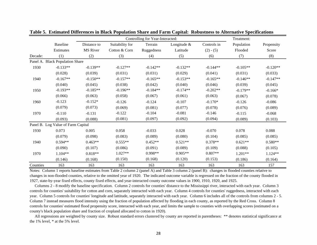
Table 5. Estimated Differences in Black Population Share and Farm Capital: Robustness to Alternative SpecificationsTreatment:

Baseline Distance to Suitability for Terrain Longitude & Controls in Population Propensity

Estimates MS River Cotton & Corn Ruggedness Latitude (2) - (5) Flooded Score

Decade: (1) (2) (3) (4) (5) (6) (7) (8)

1930 -0.133** -0.139** -0.127** -0.142** -0.132** -0.144** -0.105** -0.120**

(0.028) (0.039) (0.031) (0.031) (0.029) (0.041) (0.031) (0.033)

1940 -0.167** -0.150** -0.157** -0.165** -0.153** -0.165** -0.146** -0.147**

(0.040) (0.045) (0.038) (0.042) (0.040) (0.046) (0.039) (0.045)

1950 -0.193** -0.185** -0.196** -0.184** -0.174** -0.202** -0.179** -0.166*(0.066) (0.063) (0.058) (0.067) (0.061) (0.063) (0.067) (0.078)

1960 -0.123 -0.152* -0.126 -0.124 -0.107 -0.170* -0.126 -0.086(0.079) (0.073) (0.069) (0.081) (0.077) (0.078) (0.076) (0.089)

1970 -0.110 -0.131 -0.122 -0.104 -0.081 -0.146 -0.115 -0.068

(0.093) (0.088) (0.081) (0.097) (0.092) (0.094) (0.089) (0.103)

1930 0.073 0.005 0.058 -0.033 0.028 -0.070 0.078 0.088

(0.079) (0.098) (0.083) (0.089) (0.080) (0.104) (0.085) (0.085)

1940 0.594** 0.463** 0.555** 0.452** 0.521** 0.378** 0.621** 0.580**

(0.090) (0.107) (0.086) (0.091) (0.089) (0.109) (0.088) (0.105)

1970 1.104** 0.818** 1.027** 0.998** 0.905** 0.807** 1.201** 1.124**

(0.146) (0.168) (0.150) (0.168) (0.120) (0.153) (0.186) (0.164)

Counties 163 163 163 163 163 163 163 157

Panel A. Black Population Share

Panel B. Log Value of Farm Capital

Controlling for Year-Interacted:

Notes: Column 1 reports baseline estimates from Table 2 column 2 (panel A) and Table 3 column 2 (panel B): changes in flooded counties relative to changes in non-flooded counties, relative to the omitted year of 1920. The indicated outcome variable is regressed on the fraction of the county flooded in 1927, state-by-year fixed effects, county fixed effects, and year-interacted county outcome values in 1900, 1910, 1920, and 1925. Columns 2 - 8 modify the baseline specification. Column 2 controls for counties' distance to the Mississippi river, interacted with each year. Column 3 controls for counties' suitability for cotton and corn, separately interacted with each year. Column 4 controls for counties' ruggedness, interacted with each year. Column 5 controls for counties' longitude and lattitude, separately interacted with each year. Column 6 includes all of the controls from columns 2 - 5. Column 7 instead measures flood intensity using the fraction of population affected by flooding in each county, as reported by the Red Cross. Column 8 controls for counties' estimated flood propensity score, interacted with each year, and limits the sample to counties with overlapping scores (estimated on a county's black population share and fraction of cropland allocated to cotton in 1920). All regressions are weighted by county size. Robust standard errors clustered by county are reported in parentheses: ** denotes statistical significance at the 1% level, * at the 5% level.

28

Table 6. Estimated Differences in Black Population and Population: Robustness to Alternative SpecificationsTreatment:

Baseline Distance to Suitability for Terrain Longitude & Controls in Population Propensity

Estimates MS River Cotton & Corn Ruggedness Latitude (2) - (5) Flooded Score

Decade: (1) (2) (3) (4) (5) (6) (7) (8)

1930 -0.137** -0.139* -0.122* -0.172** -0.167** -0.170* -0.165** -0.143**

(0.045) (0.070) (0.053) (0.054) (0.047) (0.076) (0.043) (0.049)

1940 -0.075 -0.060 -0.033 -0.125 -0.107 -0.107 -0.108 -0.071

(0.059) (0.074) (0.069) (0.067) (0.059) (0.083) (0.062) (0.064)

1950 -0.153 -0.194 -0.111 -0.181 -0.213* -0.218 -0.218* -0.092(0.083) (0.106) (0.092) (0.098) (0.084) (0.115) (0.086) (0.087)

1960 -0.189 -0.286* -0.141 -0.199 -0.272* -0.277 -0.285* -0.089(0.108) (0.135) (0.114) (0.126) (0.106) (0.141) (0.110) (0.112)

1970 -0.307* -0.385* -0.273* -0.278 -0.380** -0.344* -0.408** -0.146

(0.131) (0.164) (0.128) (0.151) (0.129) (0.165) (0.134) (0.136)

1930 -0.018 -0.015 -0.011 -0.029 -0.030 -0.024 -0.060 -0.022

(0.054) (0.066) (0.062) (0.058) (0.050) (0.072) (0.055) (0.061)

1940 0.044 0.038 0.061 0.026 0.026 0.029 0.014 0.055

(0.065) (0.075) (0.070) (0.069) (0.062) (0.078) (0.069) (0.073)

1950 0.045 -0.038 0.051 0.027 -0.001 -0.042 -0.003 0.070

(0.096) (0.106) (0.099) (0.104) (0.091) (0.110) (0.095) (0.103)

1960 0.003 -0.118 0.006 -0.018 -0.065 -0.112 -0.060 0.020

(0.133) (0.148) (0.131) (0.145) (0.131) (0.149) (0.130) (0.138)

1970 -0.045 -0.192 -0.063 -0.067 -0.126 -0.186 -0.113 -0.049

(0.153) (0.180) (0.148) (0.167) (0.152) (0.176) (0.147) (0.153)

Counties 163 163 163 163 163 163 163 157

Controlling for Year-Interacted:

Panel A. Log Black Population

Panel B. Log Population

Notes: Column 1 reports baseline estimates from Table 2 column 4 (panel A) and column 6 (panel B): changes in flooded counties relative to changes in non-flooded counties, relative to the omitted year of 1920. The indicated outcome variable is regressed on the fraction of the county flooded in 1927, state-by-year fixed effects, county fixed effects, and year-interacted county outcome values in 1900, 1910, 1920, and 1925. Columns 2 - 8 modify the baseline specification, as described in notes to Table 5. All regressions are weighted by county size. Robust standard errors clustered by county are reported in parentheses: ** denotes statistical significance at the 1% level, * at the 5% level.

29

Table 7. Estimated Differences in Mules and Horses, Tractors, and Farm Size: Robustness to Alternative SpecificationsTreatment:

Baseline Distance to Suitability for Terrain Longitude & Controls in Population Propensity

Estimates MS River Cotton & Corn Ruggedness Latitude (2) - (5) Flooded Score

Decade: (1) (2) (3) (4) (5) (6) (7) (8)

1930 0.130** 0.092 0.128** 0.080 0.106* 0.048 0.112 0.080(0.049) (0.055) (0.047) (0.054) (0.047) (0.057) (0.057) (0.057)

1940 0.182** 0.185* 0.200** 0.126 0.148* 0.155* 0.184* 0.224**(0.067) (0.078) (0.068) (0.068) (0.065) (0.075) (0.087) (0.075)

1954 -0.250 -0.364* -0.199 -0.218 -0.328** -0.242 -0.231 -0.164(0.135) (0.159) (0.138) (0.140) (0.111) (0.127) (0.154) (0.151)

1960 -0.610** -0.672** -0.553** -0.469** -0.675** -0.460** -0.563** -0.507**(0.139) (0.166) (0.142) (0.143) (0.118) (0.135) (0.144) (0.158)

1930 0.629** 0.589** 0.571** 0.566** 0.597** 0.473* 0.648** 0.396*(0.145) (0.182) (0.158) (0.175) (0.146) (0.193) (0.166) (0.188)

1940 1.411** 1.254** 1.177** 1.184** 1.372** 0.951** 1.409** 0.776**(0.229) (0.282) (0.213) (0.259) (0.208) (0.261) (0.256) (0.252)

1954 0.846** 0.596* 0.712** 0.607** 0.783** 0.403 0.820** 0.694**(0.189) (0.230) (0.175) (0.210) (0.189) (0.209) (0.237) (0.220)

1970 0.711** 0.574** 0.553** 0.595** 0.659** 0.455* 0.719** 0.600**(0.177) (0.220) (0.169) (0.197) (0.177) (0.204) (0.224) (0.209)

1930 -0.013 0.015 -0.025 0.012 0.025 0.037 0.030 -0.013(0.050) (0.058) (0.050) (0.054) (0.053) (0.058) (0.052) (0.046)

1940 0.026 0.130 0.087 0.024 0.116 0.185* 0.064 -0.033(0.074) (0.076) (0.073) (0.079) (0.074) (0.082) (0.082) (0.072)

1954 0.342** 0.463** 0.465** 0.354** 0.473** 0.609** 0.326** 0.226*(0.109) (0.108) (0.097) (0.116) (0.097) (0.106) (0.114) (0.105)

1970 0.581** 0.532** 0.775** 0.521** 0.760** 0.723** 0.508** 0.374**(0.151) (0.167) (0.139) (0.160) (0.140) (0.160) (0.163) (0.139)

Counties 163 163 163 163 163 163 163 157

Controlling for Year-Interacted:

Panel A. Log Number of Mules and Horses

Panel B. Log Number of Tractors

Panel C. Log Average Farm Size

Notes: Column 1 reports baseline estimates from Table 3 column 4 (panel A), column 6 (panel B), and column 8 (panel C). Columns 2 - 8 modify the baseline specification, as described in notes to Table 5. Panel B includes 162 or 156 counties. All regressions are weighted by county size. Robust standard errors clustered by county are reported in parentheses: ** denotes statistical significance at the 1% level, * at the 5% level.

30

Table 8. Estimated Differences in Farmland and Value of Farmland: Robustness to Alternative SpecificationsTreatment:

Baseline Distance to Suitability for Terrain Longitude & Controls in Population Propensity

Estimates MS River Cotton & Corn Ruggedness Latitude (2) - (5) Flooded Score

Decade: (1) (2) (3) (4) (5) (6) (7) (8)

1930 0.071 0.022 0.060 0.014 0.050 -0.023 0.094* 0.052(0.042) (0.047) (0.042) (0.047) (0.039) (0.046) (0.046) (0.049)

1940 0.277** 0.251** 0.276** 0.216** 0.242** 0.203** 0.310** 0.256**(0.059) (0.062) (0.053) (0.064) (0.055) (0.058) (0.068) (0.063)

1954 0.513** 0.438** 0.499** 0.460** 0.437** 0.408** 0.534** 0.471**(0.094) (0.114) (0.095) (0.104) (0.079) (0.100) (0.123) (0.104)

1970 1.079** 0.946** 1.026** 1.043** 1.002** 0.943** 1.168** 0.947**(0.154) (0.198) (0.152) (0.176) (0.141) (0.177) (0.211) (0.183)

1930 0.012 -0.023 0.011 0.001 -0.029 -0.043 -0.021 0.004(0.052) (0.058) (0.053) (0.057) (0.057) (0.064) (0.048) (0.051)

1940 -0.031 -0.089 -0.016 -0.062 -0.052 -0.110* -0.045 -0.021(0.057) (0.057) (0.051) (0.058) (0.057) (0.055) (0.057) (0.062)

1954 -0.143 -0.302** -0.180* -0.169* -0.199** -0.351** -0.186** -0.128(0.073) (0.075) (0.072) (0.078) (0.074) (0.077) (0.070) (0.081)

1970 -0.075 -0.231** -0.105 -0.119 -0.172* -0.301** -0.085 -0.057(0.070) (0.081) (0.072) (0.074) (0.073) (0.080) (0.068) (0.074)

1930 -0.026 -0.090 -0.023 -0.059 -0.082 -0.119 -0.033 -0.046(0.054) (0.061) (0.052) (0.060) (0.051) (0.065) (0.057) (0.061)

1940 0.174* 0.085 0.207** 0.115 0.109 0.055 0.186* 0.154(0.072) (0.073) (0.064) (0.077) (0.066) (0.073) (0.082) (0.081)

1954 0.288** 0.015 0.274* 0.228* 0.065 -0.042 0.272* 0.280*(0.108) (0.119) (0.111) (0.115) (0.091) (0.100) (0.126) (0.118)

1970 0.755** 0.452* 0.759** 0.681** 0.483** 0.401** 0.817** 0.752**(0.152) (0.183) (0.155) (0.166) (0.129) (0.152) (0.196) (0.180)

Counties 163 163 163 163 163 163 163 157

Controlling for Year-Interacted:

Panel A. Log Farmland

Panel B. Log Value of Agricultural Land and Buildings, per Farm Acre

Panel C. Log Value of Agricultural Land and Buildings, per County Acre

Notes: Column 1 reports baseline estimates from Table 3 column 4 (panel A), column 6 (panel B), and column 8 (panel C). Columns 2 - 8 modify the baseline specification, as described in notes to Table 5. All regressions are weighted by county size. Robust standard errors clustered by county are reported in parentheses: ** denotes statistical significance at the 1% level, * at the 5% level.

31

32  

Appendix Figure 1. Delta Land and Pine Company Profits and Cotton Production

Notes: Delta Land and Pine Company Profits and Bales per Acre are from Dong 1993. Cotton prices are from Historical Statistics of the United States. On the left axis are profits, measured in 2010 dollars. On the right axis are: cotton prices, measured in cents per pound; and cotton bales per acre, measured in units of 10.

0

50

100

150

200

250

300

-$150

-$100

-$50

$0

$50

$100

$150

1911 1916 1921 1926 1931 1936 1941 1946 1951 1956 1961

Profits (2010 dollars) Bales/Acre (10s) Cotton Price (cents/pound)

Appendix Table 1. Estimated Relative Changes in Counties within 50km of other Major Southern RiversLog Log Black Log Log Value of Log Mules Log Avg Log Log Land Val Log Land Val

Fraction Black Population Population Farm Capital & Horses Farm Size Farmland per farm acre per county acre

Decade: (1) (2) (3) (4) (5) (6) (7) (8) (9)

1930 0.009 0.018 0.008 -0.045 -0.012 0.052* 0.021 -0.013 0.001

(0.012) (0.026) (0.021) (0.038) (0.022) (0.023) (0.016) (0.027) (0.024)1935 -0.004 0.014 0.024 0.002 -0.003

(0.023) (0.030) (0.018) (0.036) (0.031)

1940 0.025 0.025 0.001 -0.092 -0.035 0.041 0.029 -0.015 -0.023

(0.016) (0.032) (0.026) (0.057) (0.028) (0.031) (0.020) (0.037) (0.034)1945 0.065 0.002 -0.042 -0.071

(0.037) (0.022) (0.041) (0.039)

1950 0.016 0.007 -0.016 0.055 -0.008 0.016 -0.031(0.023) (0.043) (0.037) (0.038) (0.026) (0.041) (0.045)

1954 -0.077 0.043 -0.006 -0.028 -0.084(0.059) (0.039) (0.031) (0.047) (0.054)

1960 -0.010 -0.011 -0.011 -0.001 0.056 -0.011 -0.042 -0.095(0.030) (0.054) (0.054) (0.066) (0.043) (0.043) (0.047) (0.064)

1964 0.078 -0.009 -0.054 -0.105

(0.047) (0.047) (0.046) (0.070)

1970 -0.016 0.003 0.003 -0.190* 0.091 -0.031 -0.020 -0.078

(0.037) (0.069) (0.069) (0.088) (0.049) (0.060) (0.041) (0.067)

Counties 243 243 243 243 243 243 243 243 243Notes: Each column reports estimated changes in the indicated outcome variable: changes in counties within 50km of a major river relative to changes in counties within 50km - 150km of a major river, relative to the omitted year of 1920 or 1925. The sample is restricted to Southern counties within 150km of a major river, excluding all counties in the main sample region (Figure 1). The indicated outcome variable is regressed on a dummy for whether the county is within 50km of a major river, state-by-year fixed effects, county fixed effects, and county outcome values in 1900, 1910, 1920, and 1925 (when available), interacted with each year. All regressions are weighted by county size. Robust standard errors clustered by county are reported in parentheses: ** denotes statistical significance at the 1% level, * at the 5% level.

33

Appendix Table 2. Estimated Changes in Counties Bordering the Flooded Region, Relative to Counties 100km AwayLog Log Black Log Log Value of Log Mules Log Log Avg Log Log Land Val Log Land Val

Fraction Black Population Population Farm Capital & Horses Tractors Farm Size Farmland per farm acre per county acre

Decade: (1) (2) (3) (4) (5) (6) (7) (8) (9) (10)

1930 0.019 0.003 0.003 0.010 -0.033 0.045 -0.022 -0.015 0.060 0.048

(0.023) (0.048) (0.035) (0.064) (0.046) (0.140) (0.027) (0.028) (0.039) (0.043)1935 -0.045 -0.029 -0.014 0.022 0.004

(0.042) (0.030) (0.037) (0.050) (0.059)

1940 0.035 0.007 0.010 -0.048 -0.078 0.260 -0.060* -0.032 0.047 0.018

(0.034) (0.057) (0.044) (0.066) (0.042) (0.218) (0.030) (0.042) (0.046) (0.055)1945 0.179 -0.035 -0.007 0.102* 0.106

(0.158) (0.040) (0.053) (0.051) (0.064)

1950 0.075 0.050 0.050 -0.078 -0.048 0.129* 0.093(0.052) (0.081) (0.074) (0.053) (0.056) (0.056) (0.063)

1954 0.052 0.084 -0.112 -0.081 0.114* 0.035(0.067) (0.117) (0.057) (0.061) (0.053) (0.068)

1960 0.101 0.068 0.064 0.077 -0.105 -0.130 0.076 -0.055(0.064) (0.107) (0.113) (0.078) (0.064) (0.073) (0.055) (0.062)

1964 -0.070 -0.116 0.151** 0.034

(0.068) (0.082) (0.053) (0.074)

1970 0.102 0.077 0.094 -0.036 0.046 -0.001 -0.111 0.118** 0.027

(0.076) (0.127) (0.140) (0.084) (0.121) (0.064) (0.111) (0.042) (0.099)

Counties 94 94 94 94 94 94 94 94 94 94Notes: Each column reports estimated changes in the indicated outcome variable: changes in counties bordering the flooded region relative to changes in counties 100km from the flooded region, relative to the omitted year of 1920 or 1925. The sample is restricted to the 94 main sample counties with no flooding (Figure 1). The indicated outcome variable is regressed on the (negative) distance from the flooded region in 100km units, state-by-year fixed effects, county fixed effects, and county outcome values in 1900, 1910, 1920, and 1925 (when available), interacted with each year. All regressions are weighted by county size. Robust standard errors clustered by county are reported in parentheses: ** denotes statistical significance at the 1% level, * at the 5% level.

34