when we think only of sincerely helping all others, not ourselves, we will find that we receive all...

When we think only of sincerely helping all others, not ourselves, We will find that we receive all that we wish for.1 multiple comparisons

Chapter 9: Multiple Comparisons

Error rate of controlPairwise comparisonsComparisons to a controlLinear contrasts

2 multiple comparisons

Multiple Comparison Procedures

Once we reject H0: ==...t in favor of H1: NOT all ’s are equal, we don’t yet know the way in which they’re not all equal, but simply that they’re not all the same. If there are 4 columns (levels), are all 4 ’s different? Are 3 the same and one different? If so, which one? etc.


These “more detailed” inquiries into the process are called MULTIPLE COMPARISON PROCEDURES.

Errors (Type I):

We set up “” as the significance level for a hypothesis test. Suppose we test 3 independent hypotheses, each at = .05; each test has type I error (rej H0 when it’s true) of .05. However, P(at least one type I error in the 3 tests) = 1-P( accept all ) = 1 - (.95)3 .14 3, given true


In other words, Probability is .14 that at least one type one error is made. For 5 tests, prob = .23.Question - Should we choose = .05, and suffer (for 5 tests) a .23 Experimentwise Error rate (“a” or E)?

OR

Should we choose/control the overall error rate, “a”, to be .05, and find the individual test by 1 - (1-)5 = .05, (which gives us = .011)?

5multiple comparisons

The formula 1 - (1-)5 = .05

would be valid only if the tests are independent; often they’re not.

[ e.g., 1=22= 3, 1= 3

IF accepted & rejected, isn’t it more likely that rejected? ]

1 2

21

3

3


When the tests are not independent, it’s usually very difficult to arrive at the correct for an individual test so that a specified value results for the experimentwise error rate (or called family error rate).

Error Rates


There are many multiple comparison procedures. We’ll cover only a few.

Pairwise Comparisons

Method 1: (Fisher Test) Do a series of pairwise t-tests, each with specified value (for individual test).

This is called “Fisher’s LEAST SIGNIFICANT DIFFERENCE” (LSD).


Example: Broker Study

A financial firm would like to determine if brokers they use to execute trades differ with respect to their ability to provide a stock purchase for the firm at a low buying price per share. To measure cost, an index, Y, is used.

Y=1000(A-P)/AwhereP=per share price paid for the stock;A=average of high price and low price per share, for the day.“The higher Y is the better the trade is.”9 multiple comparisons

}1

1235-112

5 6

27

1713117

17 12

381743

7 5

524131418141917

n=6

CoL: broker

421101512206

14

Five brokers were in the study and six trades were randomly assigned to each broker.


= .05, FTV = 2.76

(reject equal column MEANS)

Source SSQ df MSQ FCol

Error

640.8

530

4

25

160.2

21.2

7.56

“MSW”


0

For any comparison of 2 columns,

/2/2

CL Cu

Yi -Yj

AR: 0+ t/2 x MSW x 1 + 1

ni njdfw(ni = nj = 6, here)

MSW : Pooled Variance, the estimate for the common variance


In our example, with=.05

0 2.060 (21.2 x 1 + 1 )0 5.48

6 6

This value, 5.48 is called the Least Significant Difference (LSD).

When same number of data points, n, in each column, LSD = t/2 x 2xMSW

.n


Col: 3 1 2 4 5 5 6 12 14 17

Summarize the comparison results. (p. 443)

1. Now, rank order and compare:

Underline Diagram


Step 2: identify difference > 5.48, and mark accordingly:

5 6 12 14 173 1 2 4 5

3: compare the pair of means within each subset:Comparison difference vs. LSD

3 vs. 12 vs. 42 vs. 54 vs. 5

**

*

<<<<

* Contiguous; no need to detail

5


Conclusion : 3, 1 2, 4, 5

Can get “inconsistency”: Suppose col 5 were 18:

3 1 2 4 5 5 6 12 14 18

Now: Comparison |difference| vs. LSD3 vs. 12 vs. 42 vs. 54 vs. 5

* *

*

<<><

Conclusion : 3, 1 2 4 5 ???

6


• Broker 1 and 3 are not significantly different but they are significantly different to the other 3 brokers.

Conclusion : 3, 1 2 4 5

• Broker 2 and 4 are not significantly different, and broker 4 and 5 are not significantly different, but broker 2 is different to (smaller than) broker 5 significantly.


MULTIPLE COMPARISON TESTING

AFS BROKER STUDYBROKER ----> 1 2 3 4 5TRADE 1 12 7 8 21 24 2 3 17 1 10 13 3 5 13 7 15 14 4 -1 11 4 12 18 5 12 7 3 20 14 6 5 17 7 6 19

COLUMN MEAN 6 12 5 14 17

ANOVA TABLE

SOURCE SSQ DF MS Fcalc

BROKER 640.8 4 160.2 7.56

ERROR 530 25 21.2


Fisher's pairwise comparisons (Minitab)

Family error rate = 0.268

Individual error rate = 0.0500

Critical value = 2.060 t_/2

Intervals for (column level mean) - (row level mean)

1 2 3 4

2 -11.476

-0.524

3 -4.476 1.524

6.476 12.476

4 -13.476 -7.476 -14.476

-2.524 3.476 -3.524

5 -16.476 -10.476 -17.476 -8.476

-5.524 0.476 -6.524 2.476

Minitab: Stat>>ANOVA>>One-Way Anova then click “comparisons”.

Col 1 < Col 2

Cannot reject Col 2 = Col 4


Pairwise comparisons

Method 2: (Tukey Test) A procedure which controls the experimentwise error rate is “TUKEY’S HONESTLY SIGNIFICANT DIFFERENCE TEST ”.


Tukey’s method works in a similar way to Fisher’s LSD, except that the “LSD” counterpart (“HSD”) is not

t/2 x MSW x 1 + 1ni nj

t/2 x 2xMSWn

=or, for equal number of data points/col( ) ,

but tuk X 2xMSW ,n

where tuk has been computed to take into account all the inter-dependencies of the different comparisons.

/2


HSD = tuk/2x2MSW n

_______________________________________

A more general approach is to write

HSD = qxMSW n

where q = tuk/2 x2

--- q = (Ylargest - Ysmallest) / MSW n

---- probability distribution of q is called the

“Studentized Range Distribution”.

--- q = q(t, df), where t =number of columns,

and df = df of MSW 22multiple comparisons

With t = 5 and df = v= 25,from Table 10:

q = 4.15 for 5% tuk = 4.15/1.414 = 2.93

Then,

HSD = 4.15

alsox


In our earlier example:

Rank order:

3 1 2 4 5

5 6 12 14 17

(No differences [contiguous] > 7.80)


Comparison |difference| >or< 7.803 vs. 13 vs. 23 vs. 43 vs. 51 vs. 21 vs. 41 vs. 52 vs. 42 vs. 54 vs. 5

* <<>><>><<<

912*8

11*5*

(contiguous)

7

3, 1, 2 4, 52 is “same as 1 and 3, but also same as 4 and 5.” 25multiple comparisons

Tukey's pairwise comparisons (Minitab)


Individual error rate = 0.00706

Critical value = 4.15 q_

Intervals for (column level mean) - (row level mean)

1 2 3 4 2 -13.801 1.801 3 -6.801 -0.801 8.801 14.801 4 -15.801 -9.801 -16.801 -0.199 5.801 -1.199 5 -18.801 -12.801 -19.801 -10.801 -3.199 2.801 -4.199 4.801

Minitab: Stat>>ANOVA>>One-Way Anova then click “comparisons”.


Special Multiple Comp. Method 3: Dunnett’s test

Designed specifically for (and incorporating the interdependencies of) comparing several “treatments” to a “control.”

Example: 1 2 3 4 5

6 12 5 14 17

Col

} n=6CONTROL

Analog of LSD (=t/2 x 2 MSW )n D = Dut/2 x 2 MSW

n

From table or Minitab 27multiple comparisons

D= Dut/2 x 2 MSW/n

= 2.61 (2(21.2) )= 6.94

- Cols 4 and 5 differ from the control [ 1 ].- Cols 2 and 3 are not significantly differentfrom control.

6

In our example: 1 2 3 4 5 6 12 5 14 17

CONTROL

Comparison |difference| >or< 6.941 vs. 21 vs. 31 vs. 41 vs. 5

618

11

<< > >


Dunnett's comparisons with a control (Minitab)

Family error rate = 0.0500 controlled!!Individual error rate = 0.0152

Critical value = 2.61 Dut_/2

Control = level (1) of broker

Intervals for treatment mean minus control mean

Level Lower Center Upper --+---------+---------+---------+-----2 -0.930 6.000 12.930 (---------*--------) 3 -7.930 -1.000 5.930 (---------*--------) 4 1.070 8.000 14.930 (--------*---------) 5 4.070 11.000 17.930 (---------*---------) --+---------+---------+---------+----- -7.0 0.0 7.0 14.0

Minitab: Stat>>ANOVA>>General Linear Model then click “comparisons”.


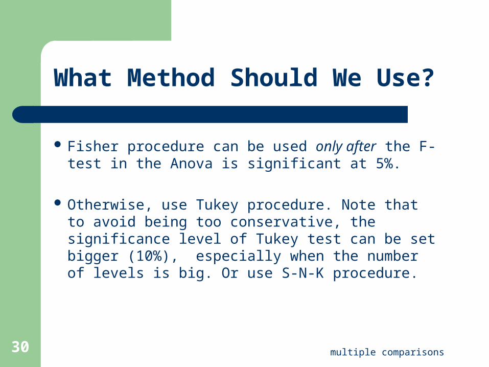
What Method Should We Use?

Fisher procedure can be used only after the F-test in the Anova is significant at 5%.

Otherwise, use Tukey procedure. Note that to avoid being too conservative, the significance level of Tukey test can be set bigger (10%), especially when the number of levels is big. Or use S-N-K procedure.


31

Consider 4 column means: Y.1 Y.2 Y.3 Y.4

6 4 1 -3

Grand Mean = Y.. = 2 # of rows (replicates) = R = 8

11 22 33 44

Consider the following data, which,let’s say, are the column means of a one factor ANOVA, with the one factorbeing “DRUG”:

Contrast

Contrast

Example 1

1 2 3 4

Placebo

Sulfa

Type

S1

Sulfa

Type

S2

Anti-biotic

Type A

Suppose the questions of interest are

(1) Placebo vs. Non-placebo

(2) S1 vs. S2

(3) (Average) S vs. A32multiple comparisons

33

• For (1), we would like to test if the mean of Placebo is equal to the mean of other levels, i.e. the mean value of {Y.1-(Y.2 +Y.3 +Y.4)/3} is equal to 0.

• For (2), we would like to test if the mean of S1 is equal to the mean of S2, i.e. the mean value of (Y.2-Y.3) is equal to 0.

• For (3), we would like to test if the mean of Types S1 and S2 is equal to the mean of Type A, i.e. the mean value of {(Y.2 +Y.3 )/2-Y.4} is equal to 0.

In general, a question of interest can be expressed by a linear combination of column means such as

with restriction that aj = 0.

Such linear combinations are called (linear) contrasts.

.j jj

Z a Y


Test if a contrast has mean 0The sum of squares for contrast Z is

where n is the number of rows (replications).

The test statistic Fcalc = SSZ/MSW is distributed as F with 1 and (df of error) degrees of freedom.

Reject E[Z]= 0 if the observed Fcalc is too large

(say, > F0.05(1,df of error) at 5% significant level).

2 2/ jj

SSZ n Z a


Example 1 (cont.): aj’s for the 3 contrasts

P vs. P: Z1

S1 vs. S2:Z2

S vs. A: Z3

1 2 3 4

-3 1 1 1

0 -1 1 0

0 -1 -1 2

P S1 S2 A


top row middle row bottom row

j

ja2

Calculating


Y.1 Y.2 Y.3 Y.4

1 1 1 5.33

0.50

8.17

0

0

Placebovs. drugs

S1 vs. S2

Average Svs. A

P S1 S2 A

14.0014.00

5 6 7 10

-1

01

-1

-1

-3

2

2 2/ jj

Z a


39

42.64

.50 4.00

8.17 65.36

14.00 112.00

5.33

(Y.j - Y..)2 = 14.

•SSBc = 14.R;•R = # rows= 8.

SSBc !

j

jaZ 22 / j

jaZ

SSZ22 /8

:

40

A set of k contrasts { Zi = , i=1,2,…,k } are called orthogonal if

Orthogonal ContrastsOrthogonal ContrastsOrthogonal ContrastsOrthogonal Contrasts

jijYa .

ai1j . ai2j = 0 for all i1, i2,

j i1 = i2.

If k = c -1 (the df of “column” term and c: # of columns), then

c

k

ii SSBSSZ

1

41

If a set of contrasts are orthogonal, their corresponding questions are called independent because the probabilities of Type I and Type II errors in the ensuing hypothesis tests are independent, and “stand alone”.

That is, the variability in Y due to one contrast (question) will not be affected by that due to the other contrasts (questions).

Orthogonal Orthogonal ContrastsContrasts

Orthogonal Orthogonal ContrastsContrasts

42

Orthogonal Orthogonal BreakdownBreakdownOrthogonal Orthogonal BreakdownBreakdown

Since SSBcol has (C-1) df (which corresponds with having C levels, or C columns ), the SSBcol

can be broken up into (C-1) individual SSQ values, each with a single degree of freedom, each addressing a different inquiry into the data’s message (one question).

A set of C-1 orthogonal contrasts (questions) provides an orthogonal breakdown.

43

Recall Data in Example 1:

{R=8

Placebo....

. 5

S1

.

.

.

. .

6

S2

.

.

.

. .

7

A....

. 10

Y..= 7

44

Source SSQ df MSQ FDrugs

Error

112

140

3

28

37.33

5

7.47

ANOVA

F1-.05(3,28)=2.95

45

An Orthogonal Breakdown

Source SSQ df MSQ F

Drugs

Error

{Z1

Z2

Z3

112{42.64 4.00 65.36

3{ 111111

42.6442.64 4.004.0065.3665.36

8.538.53 .80.8013.0713.07

140140 28 5 28 5

FF1-.051-.05(1,28)=4.20(1,28)=4.20

Example 1 (Conti.): Conclusions

The mean response for Placebo is significantly different to that for Non-placebo.

There is no significant difference between using Types S1 and S2.

Using Type A is significantly different to using Type S on average.


47

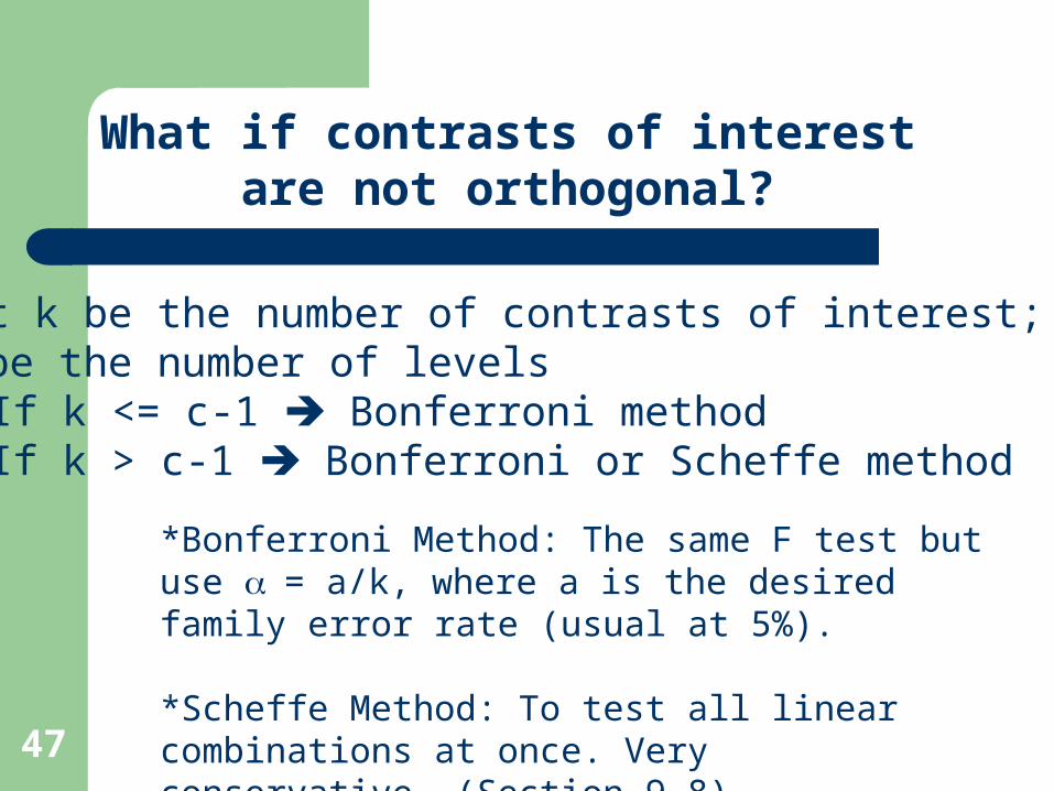
What if contrasts of interest are not orthogonal?

*Bonferroni Method: The same F test but use = a/k, where a is the desired family error rate (usual at 5%).

*Scheffe Method: To test all linear combinations at once. Very conservative. (Section 9.8)

Let k be the number of contrasts of interest; c be the number of levels1. If k <= c-1 Bonferroni method2. If k > c-1 Bonferroni or Scheffe method

48

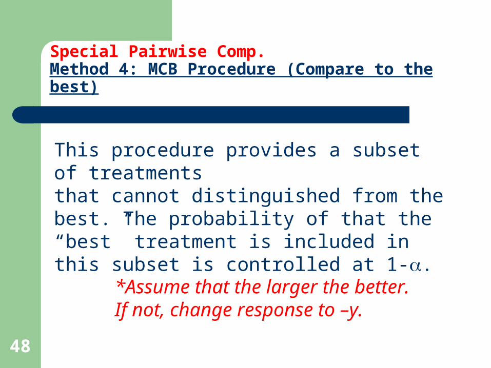
This procedure provides a subset of treatments that cannot distinguished from the best. The probability of that the “best” treatment is included in this subset is controlled at 1-.

Special Pairwise Comp.Method 4: MCB Procedure (Compare to the best)

*Assume that the larger the better.If not, change response to –y.

49

Identify the subset of the best brokers

Hsu's MCB (Multiple Comparisons with the Best)


Critical value = 2.27

Intervals for level mean minus largest of other level means

Level Lower Center Upper ---+---------+---------+---------+----1 -17.046 -11.000 0.000 (------*-------------) 2 -11.046 -5.000 1.046 (-------*------) 3 -18.046 -12.000 0.000 (-------*--------------) 4 -9.046 -3.000 3.046 (------*-------) 5 -3.046 3.000 9.046 (-------*------) ---+---------+---------+---------+---- -16.0 -8.0 0.0 8.0

Brokers 2, 4, 5

Minitab: Stat>>ANOVA>>One-Way Anova then click “comparisons”, HSU’s MCB

Not included; only if the interval (excluding ends) covers 0, this level is selected.

when we think only of sincerely helping all others, not ourselves, we will find that we receive all...

Documents

comparisons comparisons

comparisons method

multiple comparison

experimentwise error

family error rate

overall error rate

error rates

individual test