Rogue Access Point Detection

Using Innate Characteristics of the 802.11 MAC

Aravind Venkataraman and Raheem Beyah

Cigital Inc. and Georgia State University avenkataraman@cigital.com and rbeyah@cs.gsu.edu

Abstract. Attacks on wireless networks can be classified into two categories:

external wireless and internal wired. In external wireless attacks, an attacker

uses a wireless device to target the access point (AP), other wireless nodes or

the communications on the network. In internal wired attacks, an attacker or

authorized insider inserts an unauthorized (or rogue) AP into the wired

backbone for malicious activity or misfeasance. This paper addresses detecting

the internal wired attack of inserting rogue APs (RAPs) in a network by

monitoring on the wired-side for characteristics of wireless traffic. We focus on

two 802.11 medium access control (MAC) layer features as a means of

fingerprinting wireless traffic in a wired network. In particular, we study the

effect of the Distributed Coordination Function (DCF) and rate adaptation

specifications on wireless traffic by observing their influence on arrival delays.

By focusing on fundamental traits of wireless communications, unlike existing

techniques, we demonstrate that it is possible to extract wireless components

from a flow without having to train our system with network-specific wired and

wireless traces. Unlike some existing anomaly based detection schemes, our

approach is generic as it does not assume that the wired network is inherently

faster than the wireless network, is effective for networks that do not have

sample wireless traffic, and is independent of network speed/type/protocol. We

evaluate our approach using experiments and simulations. Using a Bayesian

classifier we show that we can correctly identify wireless traffic on a wired link

with 86-90% accuracy. This coupled with an appropriate switch port policy

allows the identification of RAPs.

Keywords: Rogue Access Point Detection, 802.11 MAC Protocol, Rate

Adaptation, Distributed Coordination Function

1 Introduction

A dangerous insider attack is one where cheaply available APs are illicitly plugged

into the network with the motivation of extending connectivity. Like other insider

attacks, the AP stays invisible to a firewall as it is actually behind it, thus making it

difficult to detect. Hence, the AP creates a back door for attackers, obviating the need

to go through the firewall. This paper presents a practical solution for this attack

which can happen in one of two scenarios - wired networks with or without existing

legitimate APs.

The core of our detection scheme is an agent sitting atop a switch, or a separate

monitoring device that is connected to the mirror port of a switch, that passively sniffs

passing traffic streams on the wired-side. Using inherent differences in wireless

characteristics as compared to wired traffic, this agent is able to deem the originating

link as being wired or wireless. This inference is then followed up with a switch port

AP authorization policy to differentiate between rogue and legitimate APs.

Though some of the existing methods work with proven efficacy, they do not try to

exploit the underlying facets of the wireless MAC protocol to detect RAPs, but

instead attempt to classify wireless traffic based on the greater delay observed in

network statistics (e.g., round-trip-time (RTT), inter-packet arrival time (IAT)). This

is based on an assumption that the wireless link capacity will never reach that of

wired. A more general solution is needed as this may not always be the case. Also,

since many of the previous algorithms need to be trained on both wired and wireless

traffic for a given network, they cannot be used in networks without existing APs as

there would be no prior wireless trace available.

As in other wired-side detection approaches from academia1, in our method we

study the arrival pattern of upstream traffic towards the gateway router (and possibly

the Internet) for traces of the 802.11 MAC protocol. Though downstream TCP flows

are likely to occupy a significant portion of traffic on the link, our approach is not

limited in scope. This is because, as will be shown in Section 4.3, our classifier can

work with a minimal input trace. It works with an accuracy ranging from 87% to 91%

for upstream data inputs of size ranging from 250 packets to 1000 packets

respectively2. At any given time, there may be various activities that the RAP is used

for in a corporate network, such as, web browsing, email, document uploads to file

servers, etc. Web browsing contributes varying levels of upstream data - mostly in the

form of HTTP requests - depending on the content and the load of requests. When a

web site is crawled by visiting, say five URLs recursively, the amount of upstream

data generated varies from 75 data packets (for primarily text based web pages like

www.craigslist.com) up to 400 packets (for relatively graphic intensive web pages like

www.facebook.com). Further, it takes about 500 packets to deliver an email of size

750Kb and about 1000 packets to upload a file of 1.5Mb (e.g., saving a file to the

company file server). Thus, upstream monitoring is a viable option.

Our first approach exploits the collision avoidance process of the DCF in the

802.11 MAC. To avoid collisions while transmitting, a wireless node has to sense the

channel prior to an attempt at sending. Once the channel is clear, the node will wait

for a random time period (chosen from 0 time units to a fixed upper bound) before

attempting to transmit. If the node senses that the channel is occupied, or in case of a

collision, the node has to back-off exponentially before retransmitting (i.e., the fixed

upper bound increases exponentially, increasing the probability of choosing a higher

back-off value). This procedure, carrier sense multiple access with collision

avoidance (CSMA/CA), of the DCF has both fixed components and bounded random

components that can be artificially produced and used as a signature for wireless

traffic.

1 The wired-side approaches will be discussed in Section 2.

2 Refer to Figure 8, the details of which will be discussed in Section 4.4.

The second approach exploits the process of rate adaptation in the 802.11 MAC.

Rate adaptation algorithms allow wireless hosts to alter their encoding scheme

(transmission rate) to account for channel interference during transmission. When

interference is detected, the node adapts its rate and transmits at a slower rate in an

attempt at reducing packet loss. As the rate adjusts (lower or higher), there are

noticeable and unique ‘jumps’ in the packet IAT. These ‘jumps’ can be artificially

produced and used as a signature for wireless traffic.

For both of the above techniques, we show that the signature created stays intact

and can be detected on the wired-side allowing us to deem specific traffic as

originating from a wireless node.

Each of the two approaches work best in specific cases. The first approach works

best when there is little interference and the transmission rate essentially stays

constant. Intuitively, the second approach works best when the network is more

volatile as more ‘jumps’ are produced during that period. Since network stability is

unpredictable, we combine the two schemes and present a solution that accounts for

realistic, unpredictable network conditions.

The remainder of this paper is organized as follows. Section 2 outlines previous

work in RAP detection. In Section 3 we briefly illustrate why magnitude-based

approaches are not optimal. An introduction to the 802.11 MAC protocol collision

avoidance mechanism and a breakdown of the delay induced by it on wireless traffic

is presented in Section 4. A mathematical representation is derived from its inherent

mechanism following which we validate the model using a Bayesian classifier. A

similar pattern of presentation is taken in Section 5 as in Section 4, where we perform

an analysis of the manner in which rate adaptation occurs, followed by accuracy

measures of our model. In Section 6, we perform a comparative study of the two

techniques in an attempt to come up with a bridged solution. We present the

scalability of our techniques in Section 7 and conclude in Section 8.

2 Related Work

Current work on RAP detection can be classified into three categories. The first two

categories contain techniques that use the magnitude of statistics (mean, median,

entropy, etc.) of IATs and RTTs as the primary metrics for classification respectively.

The third category contains industry work that primarily make use of radio frequency

scanning to discover wireless activity within a network.

References [1-6] fall in the first category. Beyah R., et al., [1] were among the

earliest to suggest the possibility of using temporal characteristics, such as IATs, for

RAP detection. They used the IATs of data packets and TCP ACK packets to identify

the type of traffic flow. The authors in [2] take a similar approach as that taken in [1]

but extend the work by creating an automated classifier. Wei W., et al., in [3-4]

present two similar proposals that examine IATs of TCP ACK pairs to identify the

type of traffic flow. However, the use of ACK pairs limits this technique to TCP

traffic. A noteworthy effort in the area of traffic classification is [5] which attempts to

categorize different types of access links using median and entropy of packet IATs.

The approach is however not applicable to detecting RAPs because it is active

(requires probing) and requires cooperation (probe responses) from malicious nodes.

In [6], the authors create a spectral profile for WLANs based on the entropy of IATs.

They assume link quality and unpredictability of the wireless medium as the cause for

greater wireless 'uncertainty' and do not study the effect of the DCF.

In the second category, [7-9] make use of RTT as a metric for classification. Since

these methods rely on RTT, they cannot accommodate traffic streams other than TCP.

Though [7] briefly mentions the effect of the DCF, it does not go into detail to study

its mechanics. Reference [8] uses a distinctive approach for segregating network

types, complete with traffic conditioning to eliminate noise. However, it demarcates

wired and wireless traffic with the help of mean and deviation of the RTT dataset

which is not advisable as these parameters differ with varying types, speeds, and

congestion levels of networks. Their approach is claimed to be non-intrusive.

However, since it involves conditioning of traffic it is still, at minimum, pseudo-

active. In [9], although for a disparate motive and in a dissimilar context, Cheng L., et

al., were among the first to work on identifying wireless traffic for the purpose of

access link type recognition. However, their model employs a probing process to gain

information about nodes in the network and thus not likely to be of assistance in the

RAP problem space for the same reason that [5], as mentioned above, falls short.

The third category includes several industry solutions [10-17], many of which

exhibit non-scalability and limited effectiveness because of the use of either radio

frequency (RF) scanning and/or MAC address based authentication. The use of RF

scanning is not practical as the malicious user can use directional antennas, can adjust

the power of the AP as to not be detected, and in large networks it becomes analogous

to finding a needle in a haystack. The use of the MAC address as a parameter for

authentication is not appropriate because of the ease of spoofing.

Outside of the three categories, [18-20] propose hybrid frameworks consolidating

the above mentioned wired and wireless-side detection models and inherit the flaws

from each type.

As previous schemes primarily compare the relative behavior of traffic on each

link, they require traces of each class of network traffic for their scheme to be

effective. This approach is limiting, as a network without existing legitimate APs

(e.g., government labs) would not be able to easily provide a wireless trace. Further,

because many use threshold-based separation metrics, another limiting assumption

made is that wireless networks will always be slower than their wired counterparts.

As will be shown in subsequent sections, our method is free of each of the

aforementioned assumptions.

3 Problem with Magnitude-Based Classification

As mentioned in the previous section, many of the existing works focus on the

difference, in some form, of the magnitude of the IAT or RTT to differentiate wireless

from wired traffic. In this section, we illustrate, via simulation, the challenge with

these approaches as wireless speeds begin to approach that of wired traffic.

Simulations were performed using ns2 [24]. The cumulative distribution functions

(CDFs) of the IAT and RTT values are shown in Figures (1a, 1b) and (2a, 2b)

respectively. Figures 1a and 2a illustrate why the magnitude-based approaches work

when the assumption is that WLANs are slower than LANs ( IATwl, RTTwl > IATwd,

RTTwd ). However, as shown in Figures 1b and 2b, these schemes will breakdown if

the WLAN speed reaches that of the LAN ( IATwl, RTTwl IATwd, RTTwd ).

The results shown in Figures 1 and 2 were obtained from within single trials each

of 1000 packets of upstream data for various network type/speeds (LAN - 10Mbps,

100Mbps; WLAN - 11Mbps, 24Mbps). Ethernet and wireless senders were made to

send FTP data to a server one hop away on the wired-side. Simulations were

performed on a setup similar to the experimental setup that will be described in

Section 4.3.

Partially motivated by this argument against threshold based detection, we propose

an adaptable solution that makes no assumption about the link speed. In the next

section, we introduce our first scheme beginning with an introductory analysis.

4 Scheme I - DCF Based Detection

A wireless node’s packet transmission mechanism is regulated by the specifications of

the 802.11 MAC layer protocol, the Distributed Coordination Function (DCF). The

DCF employs a CSMA/CA distributed algorithm for collision avoidance. In this

method, a node that wants to transmit data on a wireless link has to wait for a fixed

duration, namely Distributed Inter Frame Space (DIFS) and a bounded random

amount of time, called back-off (σ), before using the channel. Upon receiving the

data, the node at the other end waits for a fixed period, called the Short Inter Frame

Space (SIFS), before answering with a MAC-level acknowledgment (MAC-ACK),

0 1000 2000 3000 4000 50000

0.1

0.2

0.3

0.4

0.5

0.6

0.7

0.8

0.9

1

IAT (us)

CD

F

100Mbps LAN

11Mbps WLAN

0 1000 2000 3000 4000 50000

0.1

0.2

0.3

0.4

0.5

0.6

0.7

0.8

0.9

1

IAT (us)

CD

F

10 Mbps LAN

24Mbps WLAN

0 500 1000 1500 2000 2500 30000

0.1

0.2

0.3

0.4

0.5

0.6

0.7

0.8

0.9

1

RTT (us)

CD

F

100 Mbps LAN

11 Mbps WLAN

0 500 1000 1500 2000 2500 30000

0.1

0.2

0.3

0.4

0.5

0.6

0.7

0.8

0.9

1

RTT (us)

CD

F

10Mbps LAN

24Mbps WLAN

Fig. 1. IAT distribution for (a) slower WLAN, (b) faster WLAN.

Fig. 2. RTT distribution for (a) slower WLAN, (b) faster WLAN.

and the cycle follows thereon. Further, if the channel is sensed busy or if a collision is

detected the originating node backs-off before trying again. The bounded random

delay - Contention window (CW) has an exponentially increasing upper bound to

reduce the chances of collisions.

Accordingly, the DCF has both fixed components and bounded random

components that can be artificially produced and used as a signature for wireless

traffic. The process employed for transmission in a wireless medium and the delay

between packet arrivals (IATwl) as observed at the receiver are shown in Figure 3.

Drawing from the DCF’s basic mode of operation, we deduce a pattern unique to

wireless streams that allows one to anticipate packet arrivals at known intervals. This

property enables us to artificially construct packet arrival time series that represent

wireless traffic.

4.1 Analysis

First, in order to demonstrate the effect of the DCF on the delay, we arrive at

representations for the IATs of wired and wireless networks (IATwd and IATwl).

In Equations 1 and 2, dtrans, dprop and dqueue are the transmission, propagation

and queuing delays for a network respectively. Since dtrans >> dprop, the

propagation delay is neglected in our analysis. The queuing delay dqueue plays an

important part in determining the efficacy of wired-side detection. This will be

discussed with experimental results in Section 4.3.

wdwdwdwd dqueue +dprop +dtrans = IAT (1)

wlwlwlwl dqueue +dprop +dtrans = IAT (2)

wdoverhead

dtrans +framedtrans = wddtrans (3)

randomconstant

wloverheadframewl

DCF +DCF +

dtrans +dtrans =dtrans

(4)

In Equations 3 and 4, dtransframe is the transmission time per frame; dtransoverhead is

the overhead incurred in transmitting the packet header in the wired case, and

transmitting the packet header and MAC-ACK in the wireless case.

Fig. 3. Illustration of the DCF in 802.11 networks.

ACK-MACoverhead +

pktoverhead =

wloverhead

dtrans (5)

Note that dtranswl additionally comprises of the waiting time incurred because of

the DCF, the constituents of which are shown in Equations 6 and 7.

SIFS+ DIFS =constant

DCF (6)

σ=random

DCF (7)

The fixed delay element within the DCF contributed delay is a combination of the

DIFS and SIFS periods.

The back-off (σ) is the random period for which the sender has to wait in addition

to the DIFS. This is repeated for each unsuccessful transmission attempt. The back-

off for the ith retransmission (σi) is randomly chosen from within the CWi which is an

increasing function of the number of retransmission attempts and the number of times

the channel was sensed as busy by the sender. The DCF uses an exponential

algorithm, where for each retry, the CW size is doubled starting at a lower bound

(CWmin) until a maximum value (CWmax) is reached.

( )i

CWiσ 0,∈ (8)

[ ] [ ]maxmini

maxii CW,CWmin=CW,min=CW 22CW 1− (9)

minii CWCWσ ∝∝ (10)

Hence, arrival times can be predicted as a function of CWmin in the form of a finite

random variable. This is an important result which shows that the DCF provides us

with an increasing trend for wireless links, one whose base frequency (θ) is given in

Equation 11.

[ ]

minCW+

constantDCF +

framedtrans=θ 0,/1 (11)

Equation 11 forms the basis for our scheme. Specifically, we seek to discover a

wireless segment by extracting a basic recurring pattern that exists in all wireless

streams. Further, a wireless series can be generated synthetically which spares us

from having to train a classifier with real traces.

Since the RAP environment would likely involve a single client node (the

Fig. 4. Packet arrival pattern - UDP.

Fig. 5. Packet arrival pattern - TCP.

malicious intruder), our primary focus is the case where there are minimal collisions

as a result of competing traffic in the network, and thus assume that σ varies between

0 and CWmin. We plan to address the scenario where multiple users access the RAP in

the future.

This wireless time series is not uniform for different traffic types. In light of

Equation 4, it is important to consider two transport protocols - TCP and UDP.

Figures 4 and 5 show how the IAT distribution would look for the two different

classes.

The frame transmission time for each case would differ as shown in Hypothesis

4.1.

Hypothesis 4.1

1: if trafficUDP then

2: dtransframe = dtransdata

3: else if trafficTCP then

4: dtransframe = dtransdata + dtranstcpACK

5: end if

Because of the difference in characteristics, considering an 802.11b network as an

example, the transmission delay for the two classes would follow from the

information in Table 1 (taken from [21]) as shown in Equations 12 and 13.

This difference must be factored in when modeling the traffic behavior.

σ+=

+++σ+=

wloverhead

dtrans+data

dtrans+random

DCF+constant

DCF=

wloverhead

dtrans+frame

dtrans+random

DCF+constant

DCF=

UDPwl

dtransUDP

wlIAT

1303

10215101860

≅

(12)

( )2σ1618

1021523010182σ120

2dtrans

2DCF2DCF

2dtrans2DCF2DCF

+=

+++++=

wloverhead

+

tcpACKdtrans+

datadtrans+

random+

constant=

wloverhead

+frame

dtrans+random

+constant

=

TCPwl

dtransTCP

wlIAT ≅

(13)

Note that TCP does not always have to wait for an ACK before transmitting the

next packet. In fact, when a node is transmitting TCP traffic with a congestion

window size W greater than one (that is, W>1), it is likely to exhibit UDP-like

behavior (in the form of multiple sequential packets) except for the time when it is

waiting for ACKs. In fact, in the case of upstream TCP traffic to the Internet, a node

is highly likely to transmit in bursts. Thus, TCP’s IAT distribution would resemble

that of UDP for the most part. Hence, having taken into account the frequency of

packet arrivals for both UDP in Equation 12 and the extreme-case TCP (that is, W =

1) in Equation 13, our model is scalable for all traffic types.

As part of our groundwork, we used the expression from Equation 4 - which

repeats with the frequency shown in Equation 11, combined with the expected values

for each type of WLAN (for example, the data from Table 1 was imported for a

802.11b WLAN) to artificially build a profile set. We used values for DCFconstant from

the 802.11 standard. Also, we used a pseudo random number generator to emulate

DCFrandom, where random values were generated from within a range equivalent to the

initial CW, that is, (0,CWmin).

Table 1. 802.11b MAC Transmission Overhead.

Variable Parameter Time

(µs) Formula

DCFconstant

DIFS

SIFS

50

10

2 * slot time + SIFS = 50

SIFS

DCFrandom Average σ 310 (# of slots * slot time)/2 = (31 * 20)/2 =

310

dtransframe

dtransdata

dtransTCP-ACK

1018

30

Packet size/data rate = (1400 * 8)/11 =

1018

TCP-ACK/data rate = (40 * 8)/11 = 30

dtransoverhead

overheadpkt

overheadMAC-ACK

215

10

(Preamble + PLCP hdr.)/data rate + MAC

hdr./data rate + MAC CRC bits/data rate

= (144 + 48)/1 + (30 * 8)/11 + (4 * 8)/11

= 192 + 21 + 2 = 215

MAC-ACK/data rate = (14 * 8)/11 = 10

Figures 6a and 6b display the CDF of the IAT of TCP and UDP flows generated

via experimentation and simulation, as well as those constructed artificially using

Equations 12 and 13. The figures illustrate how closely the experimental and

simulated delay distributions follow the ones artificially created.

Also from Figure 6b, while more than 90% of the sample set follows a uniform

random dispersal over the window size, a fraction of the flow tends to deviate out of

bounds. We attribute this to the overhead in the network caused by dpropwl, possible

link-layer retransmissions and packet collisions during transmission

Fig. 6. (a) CDF of IAT for UDP. (b) CDF of IAT for TCP.

0 500 1000 1500 2000 2500 3000 3500 40000

0.1

0.2

0.3

0.4

0.5

0.6

0.7

0.8

0.9

1

IAT (us)

CD

F

Simulation 802.11g

Experimental 802.11g

Analytical 802.11g

Simulation 802.11b

Experimental 802.11b

Analytical 802.11b

0 500 1000 1500 2000 2500 3000 3500 40000

0.1

0.2

0.3

0.4

0.5

0.6

0.7

0.8

0.9

1

IAT Values (us)

CD

F

Simulation 802.11g

Experimental 802.11g

Analytical 802.11g

Simulation 802.11b

Experimental 802.11b

Analytical 802.11b

To arrive at the results in Figure 6, separate TCP and UDP experiments and

simulations were performed individually for the 802.11b and 802.11g configurations.

For each transport protocol and each WLAN speed setting, 1000 data packets were

sent from the wireless client using a socket program to the wired-side server and the

IATs were recorded on the wired-side. Correspondingly, the artificial profiles each

comprise of 1000 IAT values.

The experiments that produced part of the results in Figure 6 were performed in a

lab testbed that will be discussed in Section 4.3. The simulations associated with

Figure 6 were performed in a similar setup as the lab testbed using ns2.

In this sub-section, we showed that it is possible to independently conjecture how a

wireless stream would behave in different types of networks. To demonstrate the

accuracy of the technique, a Bayesian classifier is used to compare incoming streams'

IAT distributions with the training IAT profile set. The foundation for this

classification is presented in the next sub-section.

4.2 Classification Scheme

We use a Naïve Bayes classifier which bins the IAT datasets (the artificial profiles

and experimental/simulation traces used for the purpose of testing the system),

calculates for each dataset the number of occurrences in each bin, compares the bin

frequencies of each profile with those of the trace and predicts the trace as being akin

to the profile whose frequency distribution closest resembles that of the trace. The

Chi-square Goodness of Fit test is employed to determine the fit between each profile

and the unknown trace.

The inputs are binned into ‘b’ number of bins, where b depends on the bin width

and input data size. For both the bin width and input data size, different values are

tried with the goal of optimizing 'b' to furnish maximum accuracy. Details about these

experiments will be discussed in Section 4.4.

Profiles fi are compared with an unknown sample fx based on the frequency of

occurrences in each bin. The Bayes theorem is based on the conditional probability

model, where the posterior probability is a function of the prior probability and the

likelihood.

Because the nature of incoming traffic cannot be predicted, prior probability is

unknown and is assumed equally distributed over the n profiles.

( ) n=i

fPbilityPriorProba /1 (14)

Likelihood (measure of how similar the unknown trace is to a given profile) is

calculated for each profile using a two-sample Chi-square test which is run

independently on all sample-profile bin frequency pairs.

if

xfPLikelihood (15)

Posterior probability (measure of how likely a profile is the closest match for the

unknown) is calculated as follows:

( )i

fPi

fx

fx

fi

fProbabilityPosteriorP .P = (16)

Since fx is a random variable x1,x2,…xd,

( ) ( )i

fPi

fd

x,2

x,xP=x

fi

fP ....1

(17)

( )i

fk

xd

=k

Pi

fP=x

fi

fP ∏1

.

(18)

Since the prior probability is constant, the posterior probability essentially depends

on the likelihood measures. It is derived by aggregating the Likelihood measures,

each of which is calculated using the Pearson's Chi-square test. This test estimates the

probability that an unknown distribution fits a Chi-square distribution given a null

hypothesis. This null hypothesis is rejected (or accepted) based on the probability of

the unknown trace's fit to the Chi-square distribution. This probability is determined

as a function of the Chi-square statistic which is obtained as follows:

( )∑

−

k

=ii

Pi

Pi

X=

1

/22χ

(19)

Xi and Pi are the bin frequencies of bin i of the two samples to be compared - the

unknown and a profile. Note that the profile P is the null hypothesis. In our case, P is

the synthetically created wireless profile. The Chi-square statistic is calculated over

the bin frequencies of k bins.

4.3 Experimental Setup & Validation of Wired-side Approach

In this sub-section, we discuss: (i) preliminary experiments that were performed to

validate the general idea behind our wired-side approach and (ii) the outline of the

experimental test plan we used to evaluate the system's

accuracy.

An experimental testbed was built using three Lenovo laptops, three Dell desktops,

a Netgear 10/100 Mbps Fast Ethernet switch and a Linksys 2.4Ghz 802.11b-g AP.

The laptops were made to connect to a server on the wired-side through the AP and

switch. A desktop was set up as a sink server to receive data from both LAN and

WLAN senders. The classifier resides on a desktop connected to the switch

1.2098 1.21 1.2102 1.2104 1.2106 1.2108

x 109

0

20

40

60

80

100

120

140

160

180

200

Time (us)

Pa

ck

ets

Wired-side arrival times

Wireless-side arrival times

Fig. 7. Packet arrival times on wired and wireless sides.

immediately linking the AP to the LAN.

To ensure that our technique for wired-side detection is viable, we first determined

whether the temporal characteristics of the IAT observed on the wireless link were

intact on the wired-side. It is important to check if the DCF induced delay is carried

over to the Ethernet backbone with minimal additional overhead delay added to it. In

a single hop scenario, the overhead is primarily a function of the router queuing delay

and processing delay.

The results shown in Figure 7 are a representative sample of the arrival times of

about 200 packets extracted from a trace of a total of 10,000 packets of upstream TCP

data sent from a wireless-side sender using a socket program to the wired-side server.

The arrival times on the wired-side were recorded at the receiver node. On the

wireless side, a laptop acting as a sniffer was used in promiscuous mode to capture

traffic from the wireless sender. We observed that the arrival rates were retained

albeit with a uniformly witnessed lag (as a result of router queuing) as shown in

Figure 7.

Given the simple one-hop path from the WLAN to the classifier on the wired-side,

a switch with minimal traffic load exhibits a nearly constant queuing delay (dqueue)3

which is illustrated by the nearly fixed distance between the lines in Figure 7. In

Section 7, we discuss how the model scales to networks where the classifier is placed

several hops away from the AP.

4.4 Accuracy Measures

Having visually shown why it is likely that the packet IAT from the wireless side is

carried over to the wired-side, we evaluate the scheme's accuracy in extracting the

DCF imposed delay to determine the packet's originating link.

First, we tuned the bin width and input data size to find the optimal pair - one that

maximizes True Positive Rate (TPR) and minimizes False Positive Rate (FPR). This

is followed by additional testing with the chosen optimal parameters to obtain the

system accuracy.

The classifier was tested on traces from both wired and wireless TCP/UDP data

transfers. Sample trials on the LAN were used to measure the FPR and trials on the

WLAN to measure the TPR. Trials were performed on the WLAN for both 802.11b

and 802.11g specifications by configuring the AP to operate in the required mode. For

each network type (WLAN/LAN) and protocol (TCP/UDP), 50 sets of data were fed

into the classifier. The detections from the 50 trials were used in determining

TPR/FPR measures for the classifier. This process was repeated for different bin

width and input data size combinations. The results shown in Figure 8 are an average

of the results from the TCP and UDP trials.

An optimal bin width of 500µs and input size of 1000 packets were chosen, as the

pair gives the minimum FPR of 2% and maximum TPR of 91%. On testing the

system with the chosen parameters (Bin width = 500us, Input size = 1000 packets,

and FPR = 2%) for a total of 10 additional trials, it was observed that the technique is

3 Refer to Equations 1and 2 for the definition and Section IV.A for a discussion on dqueue.

accurate in detection approximately 92% of the time for UDP and 89% of the time for

TCP traffic, as can be seen from Figure 9.

In the RAP attack scenario, the attacker would likely often hop on the connection

for short bursts of time to avoid detection. Given the attacker's short-lived stay online,

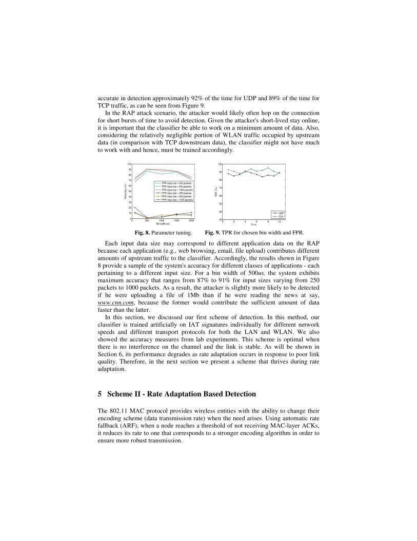
it is important that the classifier be able to work on a minimum amount of data. Also,

considering the relatively negligible portion of WLAN traffic occupied by upstream

data (in comparison with TCP downstream data), the classifier might not have much

to work with and hence, must be trained accordingly.

Each input data size may correspond to different application data on the RAP

because each application (e.g., web browsing, email, file upload) contributes different

amounts of upstream traffic to the classifier. Accordingly, the results shown in Figure

8 provide a sample of the system's accuracy for different classes of applications - each

pertaining to a different input size. For a bin width of 500us, the system exhibits

maximum accuracy that ranges from 87% to 91% for input sizes varying from 250

packets to 1000 packets. As a result, the attacker is slightly more likely to be detected

if he were uploading a file of 1Mb than if he were reading the news at say,

www.cnn.com, because the former would contribute the sufficient amount of data

faster than the latter.

In this section, we discussed our first scheme of detection. In this method, our

classifier is trained artificially on IAT signatures individually for different network

speeds and different transport protocols for both the LAN and WLAN. We also

showed the accuracy measures from lab experiments. This scheme is optimal when

there is no interference on the channel and the link is stable. As will be shown in

Section 6, its performance degrades as rate adaptation occurs in response to poor link

quality. Therefore, in the next section we present a scheme that thrives during rate

adaptation.

5 Scheme II - Rate Adaptation Based Detection

The 802.11 MAC protocol provides wireless entities with the ability to change their

encoding scheme (data transmission rate) when the need arises. Using automatic rate

fallback (ARF), when a node reaches a threshold of not receiving MAC-layer ACKs,

it reduces its rate to one that corresponds to a stronger encoding algorithm in order to

ensure more robust transmission.

0 500 1000 1500 20000

10

20

30

40

50

60

70

80

90

100

Bin width (us)

Ac

cu

racy

(%

)

TPR: Input size = 250 packets

TPR: Input size = 500 packets

TPR: Input size = 1000 packets

FPR: Input size = 250 packets

FPR: Input size = 500 packets

FPR: Input size = 1000 packets

0 2 4 6 8 1030

40

50

60

70

80

90

100

Trials

TP

R (

%)

UDP

TCP

Fig. 8. Parameter tuning. Fig. 9. TPR for chosen bin width and FPR.

As shown in [21], rate adaptation occurs regularly in WLANs because signal and

link-layer interference are common phenomena. Given that rate adaptation occurs

regularly, we seek to exploit this property that is specific to wireless streams to

distinguish them from their wired counterparts. Particularly, the switching of the

physical-layer data rate creates a variation in throughput and packet delay in a

wireless transmission that is rarely found in wired traffic. We exploit the unique

behavioral characteristics at the time of rate switching to identify wireless traffic.

In this section, we first examine the behavior of the IAT during switches in data

rate. Based on this, we derive an artificial profile for the IATs during such shifts in

data rate. The artificial profiles are incorporated into a classifier, which is then

evaluated for accuracy.

5.1 Analysis

In this sub-section, we illustrate the effect of rate adaptation on a series of packets.

Specifically, we show that there exists an IAT pattern that is exhibited only during

rate adaptation and not when a pair of successively transmitted packets is sent at a

constant physical layer data rate.

First, we visually illustrate how rate adaptation alters the arrival periods of packets

transmitted at different data rates. Figure 10 is an example representation of the

expected packet arrival sequence for a sample wireless transfer. In Figure 10, note

that the IATs vary for each rate Ri because slower rates trigger greater packet delays.

The probability Pi of the event Ri occurring depends on what we call the channel

interference index (Ω) which has a range 0↔1.

iP

ii

IAT=wl

IAT ∑ (20)

( )

( )k

Pi

PΩk<iIf

kP

iPΩk<iIf

≥→∧

≤→∧

1

0

(21)

In other words, the probability of occurrence of a lower transmission rate (in

Equation 21, rate i is lower than rate k) is inversely proportional to signal interference

and collisions. Our model safely assumes that the measure of interference Ω is not

known prior and hence Pi is unknown.

This being the case, unlike Scheme I which assumes minimal to no rate adaptation,

we choose to focus not on sets of IATi (that is, the IAT of two packets transferred at

same rate) but instead on IATj (that is, the IAT of two packets transferred at different

rates).

Fig. 10. Packet arrivals during rate adaptation.

Having abstractly shown the influence of rate adaptation on the IATs and having

settled on the idea that the inference model should be based on the IAT behavior

during the transition in data rate (IATj), we proceed to study IATj.

As shown in Figure 11, IATj is the delay during the ‘jump’ from one rate to the

next. Note that in Figure 11, IATj is of a different magnitude than IATi, where IATi is

the IAT during rate Ri and i = 1,2. Accordingly, in our classifier, we associate IATwl

with IATj. To determine which link type the test data (that exhibits IATx) belongs to,

we use the basic premise given in Hypothesis 5.1.

To illustrate the behavior of the jumps, an initial set of experiments were

performed on an 802.11b WLAN; IATs for packet pairs transmitted at the same rate

as well as different rates were extracted. In the absence of notable real channel

interference, to stimulate rate adaptation in a simple lab testbed, the experiments were

performed in the presence of a running microwave. A laptop was used as a sniffer on

the wireless-side to collect the data rates corresponding to the packets within a

transmission.

A sample of the IATs from a two minute upstream data transfer is shown in Figure

12. Although the interference resulting from the microwave usage was strong enough

to invoke rate switches down to 2Mbps and sometimes 1Mbps, for the purpose of the

current argument, the aggregated IATs of packets transmitted at 11Mbps, 5Mbps and

packets transmitted immediately after changes in data rate both ways are the only

IATs shown in Figure 12.

It can be seen in Figure 12 that the IAT distributions of the jumps fall in between

Hypothesis 5.2

1: if Ri < Ri+1 then

2: IATi > IATj > IATi+1

3: else

4: IATi < IATj < IATi+1

5: end if

Hypothesis 5.1

1: if IATx ≈ IATj then

2: Report Wireless

3: else

4: Report Wired

5: end if

Fig. 11. IAT pattern during a rate switch.

Fig. 12. IAT behavior during a rate switch –

TCP.

Fig. 13. TCP Analytical vs. Experimental

Signatures – 802.11g WLAN.

0 1000 2000 3000 4000 50000

0.1

0.2

0.3

0.4

0.5

0.6

0.7

0.8

0.9

1

IAT (us)

CD

F

11mbps

5mbps to 11mbps

11mbps to 5mbps

5mbps

0 500 1000 1500 2000 2500 3000 3500 40000

0.1

0.2

0.3

0.4

0.5

0.6

0.7

0.8

0.9

1

IAT (us)

CD

F

Experimental 36mbps to 54mbps

Analytical 36mbps to 54mbps

Experimental 54mbps to 36mbps

Analytical 54mbps to 36mbps

those of the stable rate phases before and after. This leaves us with Hypothesis 5.2.

The rationale behind this (as shown in Figure 14) is that during the transition from

R1 to R2, the MAC-level ACK is transmitted at R1 and the subsequent data frame at R2.

That is, a node which decides to reduce its data rate transmits the next data packet at

the new rate but the MAC ACK for the previous data packet would still be sent from

the AP at the old rate. Also, as can be seen from Figure 12, because of the difference

in frame and MAC ACK sizes, the IAT distribution during the jump (IATj) is biased

towards that corresponding to the rate following the jump. That is, since the frame

size >> MAC ACK size and because the data frame is sent at the new rate, IATj is

closer to the IAT associated with the new rate.

This difference in behavior during a rate switch can be exploited by studying how

it reflects on individual delay components of the corresponding IATs, as shown

below:

( ) ( )

( ) ( )1,21,2

1,21,2

pktACKMAC

randomconstantframewl

overhead+overhead+

DCF+DCF+dtrans=dtrans

−

(22)

21

2

pktACKMAC

randomconstantframej

wl

overhead+overhead+

DCF+DCF+dtrans=dtrans

−

(23)

Using Equation 23 as the base for our synthetic profiles, substituting jump-specific

dtransframe and dtransoverhead values, our classifier can be trained as shown in Figure 13.

Similar to the synthetic IAT profiles shown for the (36Mbps, 54Mbps) pair in Figure

13, multiple such jump signatures were constructed for different data rate pairs as

training sets for the classifier. Additionally, the training sets included IAT signatures

for 10Mbps and 100Mbps LANs.

5.2 Classification Scheme

The classifier used for this method is similar to the one explained in Section 4.2, with

appropriate changes made to incorporate the fact that only the IAT values during

jumps in rates are considered for training and testing as opposed to the values during a

stable rate period. In the Bayesian classifier, instead of comparing the entire trace of

IAT readings with the profiles, individual values are inspected for possible jumps.

That is, a comparison of two datasets (training and testing sets) is not required;

instead, it is sufficient to check individual incoming IAT values to see which IAT

jump signatures they are closest to.

Fig. 14. DCF behavior during a rate switch.

5.3 Experimental Setup & Validation of Wired-side Approach

The experimental setup used to validate the scheme is similar to that used for Scheme

I discussed in Section 4.3. As in [21], we use a synthetic means (microwave

interference) to force rate switching to investigate Scheme II. One of the laptops is

used as a sniffer on the wireless side, while another laptop is used to transfer data to

the wired-side desktop sink server.

To determine whether a node is switching rates when capturing packets on the

wireless side is simple, as its physical layer header contains the actual transmission

rate. However, the rate in the wireless frame is not carried over to the wired-side.

Accordingly, on the wired-side, we have to infer the rate by observing the packets’

IAT pattern. We verified that this approach is viable by capturing traffic both on the

wireless-side and the wired-side, and comparing the data rate observations made on

the wireless-side with the data rate predictions made by the classifier on the wired-

side. We observed packets that switch rates on the wireless side with a laptop acting

as a sniffer capturing promiscuously (by looking at the radiotap header in the wireless

frame) and concurrently on the wired-side by feeding captured IATs of the same

packets into the classifier. From this, we were able to determine that specific IAT

values on the wired-side correlated to confirmed rate adaptations on the wireless side.

Figure 15 gives a representative sample of the rates of the packets extracted on the

wireless side and the rates inferred by the classifier on the wired-side, illustrating the

correlation of rates of the same packets observed at both points. A total of 6000

upstream TCP data packets were transmitted with 81% of the rates predicted

correctly. It is important to note that though the accuracy of classification of the data

rates on the wired-side was 81%, the classifier is accurate in access link type

classification up to an average TPR of 97% for UDP and 91% for TCP (refer to

Figure 18). This is because even the IATs corresponding to the incorrectly inferred

rates are closer to the synthetic jump IAT profiles that the classifier was trained on as

opposed to the Ethernet IAT signatures.

The accuracy measures of the classifier used to test Scheme II are shown in the

next sub-section.

5.4 Accuracy Measures

As in Scheme I, to validate the system, the bin width used in the Bayesian binning

approach was first tuned to determine an optimum value for the classifier. Note that

0 10 20 30 40 500

2

4

6

8

10

12

Packets

Da

ta r

ate

(m

bp

s)

Wireless-side rate observations

Wired-side rate detections

Fig. 15. Rate detection on wired and wireless sides.

Scheme II operates independent of the input size as it does not compare the dataset as

a whole with the profiles and instead studies the input trace a packet at a time.

For each bin width, ten trials were performed, in each of which the classifier was

tested on TCP/UDP data packet pairs of upstream Ethernet and WLAN traffic.

TPR/FPR were generated as a function of the fraction of the input trace accurately

classified each time (Figure 16).

In order to optimize the effectiveness of this technique, we calculate what we call

the Effective Accuracy and find the optimum value that maximizes this difference

between TPR and FPR in an attempt to make a balanced trade-off between the two

metrics. For the chosen parameters (Bin width = 20µs and FPR = 14%), 12 additional

trials are run to observe the TPR distribution (Figure 17).

Note that the accuracy measures shown in Figure 17 hold for WLANs with

considerable rate adaptation. As will be shown in the next section, the accuracy of this

scheme increases as a function of the amount of interference on the network and thus

the method is not suitable for networks with minimal rate adaptation. In the next

section, we propose a technique that bridges the strengths of the two schemes

discussed so far in an effort to arrive at a comprehensive solution for normal networks

(i.e., networks with varying levels of interference).

6 Consolidated Model

While Scheme I compares input sample traces as a whole with each of the profiles,

Scheme II checks individual packet pairs within a trace for a switch in data rate. This

implies that since the input sample trace to be compared may encompass several rates,

Scheme I’s accuracy is likely to subside with increased rate adaptation. Conversely,

Scheme II will not accurately classify wireless traffic in the absence of a minimum

degree of rate adaptation.

6.1 Analysis

In an effort to present a general solution that works both when the link is stable as

Fig. 16. Bin width tuning. Fig. 17. TPR for chosen bin width and FPR.

0 100 200 300 400 50010

20

30

40

50

60

70

80

90

100

Bin width (us)

Acc

ura

cy (

%)

TPR

FPR

0 2 4 6 8 10 1220

30

40

50

60

70

80

90

100

Trials

TP

R (

%)

TCP

UDP

well as when rate adaptation occurs, we revisit the channel interference index (Ω)4

defining it as follows:

SchemeIAccuracy

SchemeIIAccuracy

Ω ∝

(24)

Equation 24 essentially captures the inverse relationship between Schemes I and II.

Scheme I works better when there is little to no interference, while Scheme II works

better during interference. Thus, it is important to consolidate the pros of the two

approaches in a way that the resulting system is effective regardless of the link

stability.

6.2 Classification Scheme

To combine the two schemes, we partition the input data set into blocks of a constant

size with the expectation that each block will be comprised of data at a specific rate.

Of course this need not be the case. So, in addition to this, we exploit the fact that

Scheme I detects the access link types of stable rate periods well and Scheme II

detects the jumps well. For the combined solution, the input trace is fed into the

classifier one block at a time. Scheme I contributes the network type/speed

observation for each of the partitions and Scheme II points out where two stable rate

periods intersect (that is, the jumps in data rate), the aggregation of which gives us the

temporal distribution of rates for a series of packet pairs. This technique is illustrated

in Figure 18, where x and y are the inferred data rates. Based on the inferred rates, the

combined scheme determines the access link type of the individual partitions. The

final access link type classification decision for the whole block of data is made as a

function of the WLAN-to-Ethernet classification ratio of individual partitions. That is,

the classifier decides between WLAN and Ethernet based on which link type is

classified in majority of the partitions. The general idea behind this unified model is

that if one of the two schemes fail, a healthy net effect is maintained as the other

scheme chips in.

6.3 Experimental Setup

The experimental setup used to test the first two schemes is employed to validate the

combined scheme. A block size of 250 packets is chosen. Accordingly, in our

experiments, each input trace of 1000 packets is partitioned into four blocks of 250

packets each.

4 Note that this metric was previously introduced in Section V.A.

Fig. 18. Depiction of combined scheme.

In the next section, we evaluate the accuracy of the combined scheme (in

comparison with that of the first two schemes) as a function of Ω by testing against

data sets that differ in the number of times rate adaptation is invoked.

6.4 Accuracy Measures

The accuracy measures of the consolidated system (in comparison with those of the

other two schemes) are shown in Figures 19.

A total of 14 trials were performed to assess how the TPR varies with an increase

in the degree of rate adaptation. This testing set comprised of 2 trials each for the 7

different degrees of rate adaptation. The degree of rate adaptation is devised as a

function of the number of switches in data rate invoked within the 1000 packet input

data set. Figure 19 shows the results of such experiments performed individually for

each of the three schemes. Results shown in Figure 19 are an average of the outcomes

from separate TCP and UDP trials. Note that the combined scheme's accuracy is not

as high as that of Scheme I. However, this technique is nonetheless effective and

unlike the initial two schemes, the combined technique is realistic as it makes no

assumption about the link quality.

7 Measure of Robustness and Scalability

In this section, we discuss how the system's performance scales to larger, more

realistic networks. We evaluate the system's scalability in two scenarios - (i) a

network where the classifier is placed multiple hops away from the AP via simulation,

and (ii) a real network (as opposed to a lab testbed).

First, to test the combined scheme’s scalability as a function of the classifier's

distance from the AP, simulations were performed where detection takes place several

hops upstream instead of the switch immediately connecting the AP to the LAN. This

is important because the AP to be detected may not always be one hop away from the

classifier node. We consider the effect of different fixed access-link and bottleneck

delays at each hop, including the best-case (1ms, 10ms, and 50ms) as well the worst-

case (300ms and 500ms) delays. The measurements observed indicate that despite a

decrease in accuracy with an increase in the distance, the system averages a worst-

case accuracy of above 60%, average-case accuracy of above 75% and best-case

accuracy of above 85% (Figure 20a). The results shown in Figure 20a were obtained

Fig. 19. Scheme accuracy comparison.

0 5 10 15 200

10

20

30

40

50

60

70

80

90

100

Number of switches in data rate

TP

R (

%)

Scheme I

Scheme II

Combined Scheme

from simulations done using ns2 and varying the number of hops between the AP and

the classifier node. The TPR measurements shown in the figure are an average of

results from 10 trials - each of 10,000 upstream data packets - performed separately

for each delay value and tested individually for a given number of hops. The 10 trials

comprised of 5 TCP and 5 UDP trials. The trace of 10,000 packets in each trial was

fed into the classifier 1000 packets at a time.

Next, we conducted experiments on a real network to arrive at the accuracy

measures of the classifier when tested with traces from a real environment. Trials

were performed on a multi-hop fiber-optic university backbone. A wireless node was

made to connect via an AP from a classroom building to the wired-side server three

blocks away in the Computer Science Department. The accuracy of the combined

scheme was measured over a total of 20 trials performed individually for TCP/UDP

data transfers and for 802.11b/g network configurations. In each trial, the classifier

was tested on a 10 minute long trace for TPR measures. As shown in Figure 20b, the

classifier is accurate up to approximately 90% of the time for UDP and 85% of the

time for TCP.

8 Conclusion and Future Work

The proposed method detects RAPs by extracting characteristics unique to a wireless

stream from network traffic. It makes use of two 802.11 MAC specifications to

fingerprint wireless attributes from the wired-side making the process simple and

scalable.

In this paper, we have studied the working and validated the accuracy of our

detection techniques in several environments. This method is immediately deployable

and is shown to scale well to realistic scenarios outside of a lab testbed. In the future,

we will continue in this direction and further test the system for robustness to other

use cases.

We plan to extend this work by scaling it to networks of greater traffic density by

taking into consideration the effect of collisions in the network as a result of multiple

users on the RAP. To this end we will study various error models and incorporate the

traffic behavior during each of these into our design. Further, we intend to study the

effect of link delay on the accuracy of the system in an attempt to derive a metric that

the classifier shall be tuned for when placed multiple hops away from the AP. Also,

we will test the system's robustness using different real network traces from publicly

available archived sources (e.g., CRAWDAD).

Further, looking ahead in RAP detection, we must assume that the misfeasor could

be tech savvy and aware of RAP defenses. To this end, we will analyze possible

Fig. 20. Multi-hop accuracy: (a) Simulation, (b) Experiment.

0 2 4 6 8 100

10

20

30

40

50

60

70

80

90

100

Number of hops

TP

R (

%)

Delay = 0.1ms

Delay = 1ms

Delay = 10ms

Delay = 50ms

Delay = 100ms

Delay = 300ms

Delay = 500ms

0 5 10 15 2030

40

50

60

70

80

90

100

Trials

TP

R (

%)

TCP - 802.11b

TCP - 802.11g

UDP - 802.11b

UDP - 802.11g

options that an attacker has to evade detection by cleverly altering his transmission

pattern. Threat strategies that an attacker may employ include reducing or increasing

his packet delay and interleaving his wireless transmissions with other types of traffic

to bypass the classifier's signatures. Note that the DCF parameters can be manipulated

in open source 802.11 drivers.

References

1. Beyah, R., Kangude, S., Yu, G., Strickland, B., and Copeland, J.: ‘Rogue access point

detection using temporal traffic characteristics.’, IEEE GLOBECOM, 2004.

2. Shetty, S., Song, M., Ma, L.: ‘Rogue Access Point Detection by Analyzing Network

Traffic Characteristics’, MILCOM, 2007.

3. Wei, W., Suh, K., Gu, Y., Wang, B., and Kurose, J.: ‘Passive online rogue access point

detection using sequential hypothesis testing with tcp ack-pairs’, IMC, 2007.

4. Wei, W., Jaiswal, S., Kurose, J., Towsley, D.: ‘Identifying 802.11 Traffic from Passive

Measurements Using Iterative Bayesian Inference.’, IEEE INFOCOM, 2006.

5. Wei, W., Wang, B., Zhg, C., Kurose, J., and Towsley, D.: ‘Classification of access

network types: Ethernet, Wireless LAN, ADSL, Cable Modem or Dialup?’, IEEE

INFOCOM, 2005.

6. Baiamonte, V., Papagiannaki, K. and Iannaccone. G.: ' Detecting 802.11 wireless hosts

from remote passive observations.', IFIP/TC6 Networking, 2007.

7. Beyah, R., Watkins, L., Corbett, C: ‘A Passive Approach to Rogue Access Point

Detection’, GLOBECOM, 2007.

8. Mano, C., Blaich, A., Liao, Q., Jiang, Y., Cieslak, D., Salyers, D., and Striegel, A.:

‘RIPPS: Rogue Identifying Packet Payload Slicer Detecting Unauthorized Wireless Hosts

Through Network Traffic Conditioning’, ACM TISSEC, 2007, Volume 11, Issue 2.

9. Cheng, L., Marsic, I.: ‘Fuzzy reasoning for wireless awareness’, International Journal of

Wireless Information Networks, 2001, Volume 8, Issue 1.

10. Bahl, P., Padhye, J., Ravindranath, L.: ‘Enhancing the Security of Corporate WI-FI

Networks Using DAIR’, ACM MobiSys, 2006.

11. http://www.netstumbler.com

12. http://www.wimetrics.com/Products/WAPD.htm

13. http://www.proxim.com/learn/library/whitepapers/Rogue_Access_Point_Detection.pdf

14. http://www.airdefense.net

15. http://www.airmagnet.com

16. http://www.airwave.com

17. http://www.cisco.com/en/US/products/sw/cscowork/ps3915

18. Chirumamilla, M.K., Ramamurthy, B.: ‘Agent based intrusion detection and response system for

wireless LANs’, ICC, 2003.

19. Ma, L., Cheng, X.: ‘A Hybrid Rogue Access Point Protection Framework for Commodity Wi-Fi Networks’. IEEE INFOCOM, 2008.

20. Songrit, S., Kitti, W., Anan, P.: 'Integrated Wireless Rogue Access Point Detection and Counterattack

System’, ISA, 2008. 21. Beyah, R., Corbett, C., Copeland, J.: ‘A Passive Approach to Wireless NIC Identification’,

ICC, 2006.

22. Bianchi, G.: ‘Performance analysis of the IEEE 802.11 distributed coordination function’,

Journal on Selected Areas of Communications, 2000, Volume 18, Issue 3.

23. Bing, B.: ‘Measured Performance of the IEEE 802.11 Wireless LAN’, LCN, 1999.

24. Chatzimisios, P., Vitsas, V., Boucouvalas, A.C.: ‘Throughput and Delay analysis of IEEE

802.11 protocol’, 5th IWNA, 2002.

25. http://www.isi.edu/nsnam/ns.