which sa are you using-baker

8/6/2019 Which Sa Are You Using-Baker

http://slidepdf.com/reader/full/which-sa-are-you-using-baker 1/20

Which Spectral Acceleration Are YouUsing?

Jack W. Baker,

a…

M.EERI, and C. Allin Cornell,

a…

M.EERI

Analysis of the seismic risk to a structure requires assessment of both therate of occurrence of future earthquake ground motions hazard and the effectof these ground motions on the structure response. These two pieces are often

linked using an intensity measure such as spectral acceleration. However, earthscientists typically use the geometric mean of the spectral accelerations of thetwo horizontal components of ground motion as the intensity measure for hazard analysis, while structural engineers often use spectral acceleration of asingle horizontal component as the intensity measure for response analysis.This inconsistency in definitions is typically not recognized when the two

assessments are combined, resulting in unconservative conclusions about theseismic risk to the structure. The source and impact of the problem is examined in this paper, and several potential resolutions are proposed. This discussion isdirectly applicable to probabilistic analyses, but also has implications for deterministic seismic evaluations. DOI: 10.1193/1.2191540

INTRODUCTION

Calculation of the risk to a structure from future earthquakes requires assessment of both the probability of occurrence of future earthquakes hazard and the resulting re-sponse of the structure due to earthquakes response. The analysis of hazard is typically

performed by earth scientists e.g., seismologists or geotechnical engineering scientists,while the analysis of response is typically performed by structural engineers. The results

from these two specialists must then be combined, and this is often done by utilizing anintensity measure IM Banon et al. 2001, Cornell et al. 2002, Moehle and Deierlein2004. Earth scientists provide the probability of occurrence of varying levels of the IM

through hazard maps or site-specific analysis, and structural engineers estimate the ef-fect of an earthquake with given levels of the IM using dynamic analysis or by associ-ating the IM with the forces or displacements applied in a static analysis .

Spectral acceleration, Sa, is the most commonly used intensity measure in practicetoday for analysis of buildings. This value represents the maximum acceleration that a

ground motion will cause in a linear oscillator with a specified natural period and damp-ing level. In fact, the true measure is pseudospectral acceleration, which is equal tospectral displacement times the square of the natural frequency, but the difference is of-

ten negligible and the name is often shortened to simply “spectral acceleration.” But Sa

is often defined differently by earth scientists and structural engineers. The differenceoriginates from the fact that earthquake ground motions at a point occur in more than

aDepartment of Civil and Environmental Engineering, Stanford University, Stanford, CA 94305-4020

293

Earthquake Spectra, Volume 22, No. 2, pages 293–312, May 2006; © 2006, Earthquake Engineering Research Institute



one direction. While structural engineers often use the Sa caused by a ground motion

along a single axis in the horizontal plane, earth scientists often compute Sa for two

perpendicular horizontal components of a ground motion, and then work with the geo-metric mean of the Sa’s of the two components. Both definitions of Sa are valid. How-ever, the difference in definitions is often not recognized when the two pieces are linked,

because both are called “spectral acceleration.” Failure to use a common definition mayintroduce an error in the results.

In this paper, the differences in these two definitions are examined, along with the

reasons why earth scientists and structural engineers choose their respective definitions.Examples of the use of these definitions are presented, along with the potential impact of failing to recognize the discrepancy. Several procedures for addressing the problem areexamined, and the relative advantages and disadvantages of each are considered. Analy-sis is sometimes performed for each axis of a structure independently, and other times an

entire 3-D structural model is analyzed at once. Both of these cases are considered, and

consistent procedures for each are described. These procedures should be helpful for analysts performing seismic risk assessments of structures.

SPECTRAL ACCELERATION: TWO DEFINITIONS

TREATMENT OF SPECTRAL ACCELERATION BY EARTH SCIENTISTS

The earth scientist’s concern with spectral acceleration is in predicting the distribu-

tion of spectral acceleration at a site, given an earthquake with a specified magnitude,distance, faulting style, local soil classification, etc. This prediction is made in the formof an attenuation model. Many attenuation models are empirically developed usinganalysis of recorded ground motions see Abrahamson and Silva 1997, Boore et al.1997, Campbell 1997, Sadigh et al. 1997, and Spudich et al. 1999, among many others.

There is scatter in this recorded data due to path effects, variation in stress drop, and other factors that are not captured by the attenuation model, which must be dealt withduring development of the attenuation model.

The observed variability in spectral acceleration is well represented by a lognormaldistribution Abrahamson 1988, 2000. Thus, attenuation models work with the mean

and standard deviation of the logarithm of Sa, which can be represented by a Gaussiandistribution. The broad variability of the distribution hinders estimation of the mean

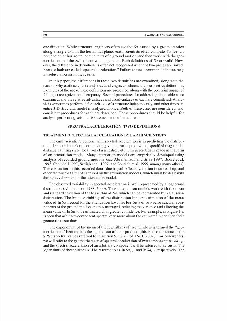
value of ln Sa needed for the attenuation law. The log Sa’s of two perpendicular components of the ground motion are thus averaged, reducing the variance and allowing the

mean value of ln Sa to be estimated with greater confidence. For example, in Figure 1 itis seen that arbitrary-component spectra vary more about the estimated mean than their

geometric mean does.

The exponential of the mean of the logarithms of two numbers is termed the “geo-metric mean” because it is the square root of their product this is also the same as theSRSS spectral values referred to in section 9.5.7.2.2 of ASCE 2002. For conciseness,

we will refer to the geometric mean of spectral acceleration of two components as Sa g .m.,

and the spectral acceleration of an arbitrary component will be referred to as Saarb. The

logarithms of these values will be referred to as ln Sa g .m. and ln Saarb, respectively. The

294 J. W. BAKER AND C. A. CORNELL



terms Sa and ln Sa will be used to refer to spectral acceleration and its logarithm, with-

out specification as to which definition is used. And the standard deviation of ln Sa will

be referred to as the “dispersion” of Sa, following common practice elsewhere. It isnoted again that these values are functions of the period and damping level specified, but

this is not stated explicitly in the notation because consideration of a particular period and damping are not needed for this discussion.

Attenuation models typically provide a predicted mean and standard deviation for

the conditional random variable ln Sa g .m., given an earthquake magnitude, distance, etc.These estimates for ln Sa g .m. can be made directly from the data, because the averaging

of the two components transformed the observed data into values of Sa g .m.. For a given

earthquake, the mean of the conditional random variable ln Saarb is equal to the mean of ln Sa g .m.. But the standard deviation of ln Saarb is greater than that of ln Sa g .m. by a fac-

tor that could be as large as 2 if the two components were uncorrelated because the

Figure 1. Response spectra from the magnitude 6.2 Chalfant Valley earthquake recorded at

Bishop LADWP, 9.2 km from the fault rupture. Response spectra for the two horizontal components of the ground motion, the geometric mean of the response spectra, and the predicted

mean for the given magnitude and distance using the prediction of Abrahamson and Silva

1997.

WHICH SPECTRAL ACCELERATION ARE YOU USING? 295



standard deviation of the mean of 2 uncorrelated random variables with common stan-

dard deviation is equal to /2. Calculating the standard deviation of ln Saarb thus

takes an additional step of going back to the non-averaged data and examining the stan-dard deviation there. Some researchers e.g., Boore et al. 1997, Spudich et al. 1999 havetaken this step, but many others have not because it was not recognized as important.However, the difference in standard deviations is in fact relevant for ground motion haz-ard analysis, as will be seen in the next section.

Deterministic Ground Motion Hazard Analysis

The effect of the standard deviation of ln Sa is easily seen in deterministic seismichazard analysis. Often in a deterministic hazard analysis, a target spectral accelerationfor a “Maximum Considered Event” is computed by specifying a scenario event mag-

nitude and distance, and then computing the value of ln Sa, at a given period and damp-ing level, that is one standard deviation greater than the mean prediction for that event

Reiter 1990, Anderson 1997. But the value of the standard deviation depends uponwhether Sa g .m. or Saarb is being used as the IM. Because of its greater dispersion loga-

rithmic standard deviation, the target value of Saarb will thus be larger than that for Sa g .m.. So the target spectral acceleration depends on the definition of Sa being used,

even though both definitions have the same mean value of ln Sa. For a “mean plus one

sigma” ground motion, Saarb will thus be larger than that for Sa g .m. by a factor of

exp ln Saarb− ln Sa g .m.

. For example, using the model of Boore et al. 1997, Boore

2005, this difference is exp0.047 at a period of 0.8 seconds with 5% damping, im-

plying that if Saarb is to be used as the IM, the target spectral acceleration would be

about 5% larger than if Sa g .m. is used.

Another method used in deterministic hazard maps is to take as the hazard value150% of the median spectral acceleration value for a characteristic event ASCE 2002.

One of the justifications for the 150% rule is that this will capture a reasonable fractionof the Sa values that could result from occurrence of this characteristic event. However,the fraction captured will vary based on which of the two definitions is used. Consider

Sa at a period of 0.8 seconds. Per the Boore et al. 1997, Boore 2005 attenuation rela-

tionship used above, Saarb has a 23% chance of exceeding 150% of the median Sa value

given the event, while Sa g .m. has a 21% chance of exceeding 150% of the median Sagiven the event. Thus the level of conservatism resulting from this rule varies slightly

depending on the Sa definition used. Spectral acceleration is merely a tool used to sim- plify the analysis problem; therefore the factor of safety should not vary based on the

definition used. In principle the 150% rule for Sa g .m. should be a “156% rule” for Saarb,in order to provide the same level of conservatism.

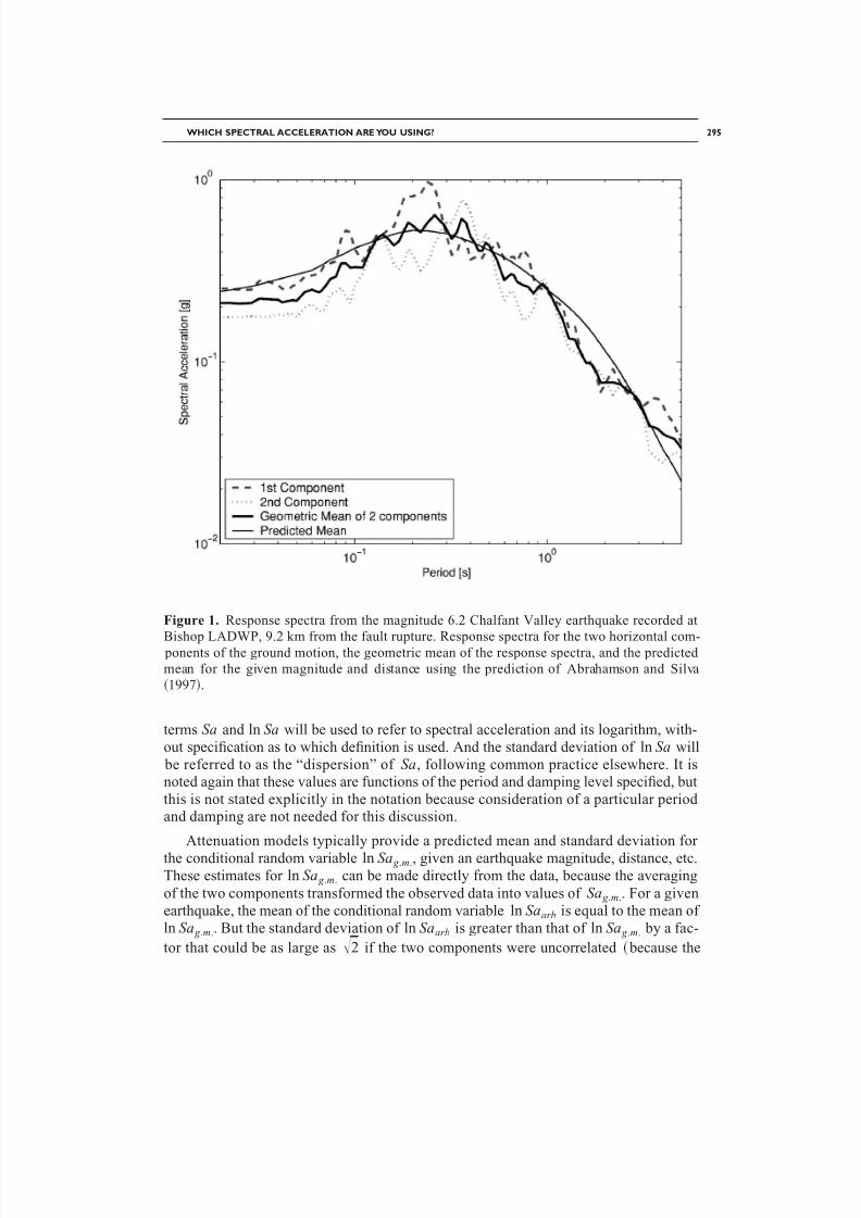
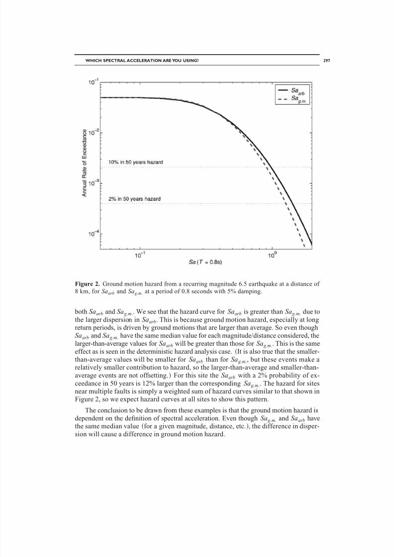
Probabilistic Ground Motion Hazard AnalysisThe variation in standard deviation is also seen in probabilistic seismic hazard analy-

sis. In Figure 2, hazard curves for the two definitions of Sa are shown for a hypothetical

site 8 kilometers away from a recurring magnitude 6.5 earthquake this simple hazard environment is representative of sites near a single large fault. Again the attenuationmodel of Boore et al. 1997, Boore 2005 is used, because it provides dispersions for




both Saarb and Sa g .m.. We see that the hazard curve for Saarb is greater than Sa g .m. due to

the larger dispersion in Saarb. This is because ground motion hazard, especially at longreturn periods, is driven by ground motions that are larger than average. So even thoughSaarb and Sa g .m. have the same median value for each magnitude/distance considered, the

larger-than-average values for Saarb will be greater than those for Sa g .m.. This is the same

effect as is seen in the deterministic hazard analysis case. It is also true that the smaller-

than-average values will be smaller for Saarb than for Sa g .m., but these events make arelatively smaller contribution to hazard, so the larger-than-average and smaller-than-

average events are not offsetting. For this site the Saarb with a 2% probability of ex-

ceedance in 50 years is 12% larger than the corresponding Sa g .m.. The hazard for sites

near multiple faults is simply a weighted sum of hazard curves similar to that shown inFigure 2, so we expect hazard curves at all sites to show this pattern.

The conclusion to be drawn from these examples is that the ground motion hazard is

dependent on the definition of spectral acceleration. Even though Sa g .m. and Saarb havethe same median value for a given magnitude, distance, etc., the difference in disper-

sion will cause a difference in ground motion hazard.

Figure 2. Ground motion hazard from a recurring magnitude 6.5 earthquake at a distance of

8 km, for Saarb and Sa g .m. at a period of 0.8 seconds with 5% damping.




This result is important, because it means that ground motion hazard cannot be used

interchangeably for both Saarb and Sa g .m.. This brings to light a problem with the U.S.

Geological Survey maps of spectral acceleration hazard Frankel et al. 2002. The mapsare produced using results from several attenuation models, some of which emphasize

the dispersion in Saarb, and some of which provide only dispersion for Sa g .m.. The U.S.Geological Survey has used the dispersions emphasized by the models’ authors, result-ing in a mix of both definitions being used. Thus the current maps are not strictly inter-

pretable as the ground motion hazard for either Saarb, or Sa g .m.. This will be addressed infuture revisions to the maps, in light of the new recognition of the importance of this

issue Frankel 2004.

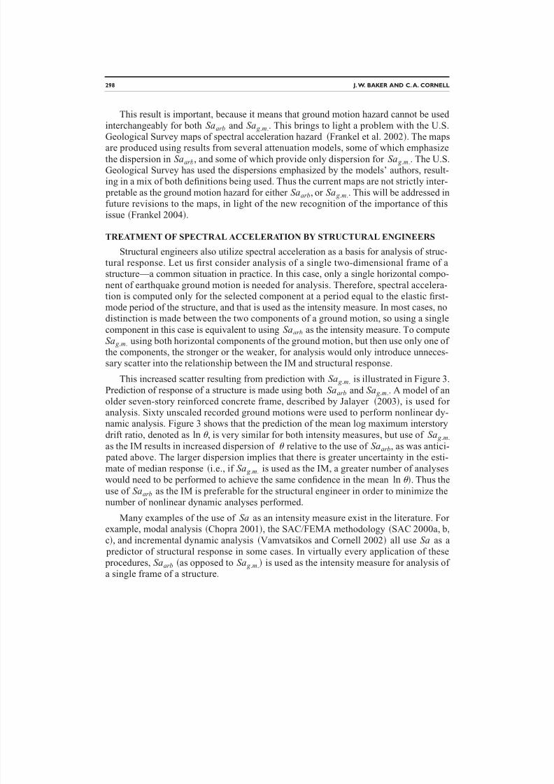
TREATMENT OF SPECTRAL ACCELERATION BY STRUCTURAL ENGINEERS

Structural engineers also utilize spectral acceleration as a basis for analysis of struc-tural response. Let us first consider analysis of a single two-dimensional frame of a

structure—a common situation in practice. In this case, only a single horizontal compo-nent of earthquake ground motion is needed for analysis. Therefore, spectral accelera-tion is computed only for the selected component at a period equal to the elastic first-mode period of the structure, and that is used as the intensity measure. In most cases, nodistinction is made between the two components of a ground motion, so using a single

component in this case is equivalent to using Saarb as the intensity measure. To computeSa g .m. using both horizontal components of the ground motion, but then use only one of the components, the stronger or the weaker, for analysis would only introduce unneces-sary scatter into the relationship between the IM and structural response.

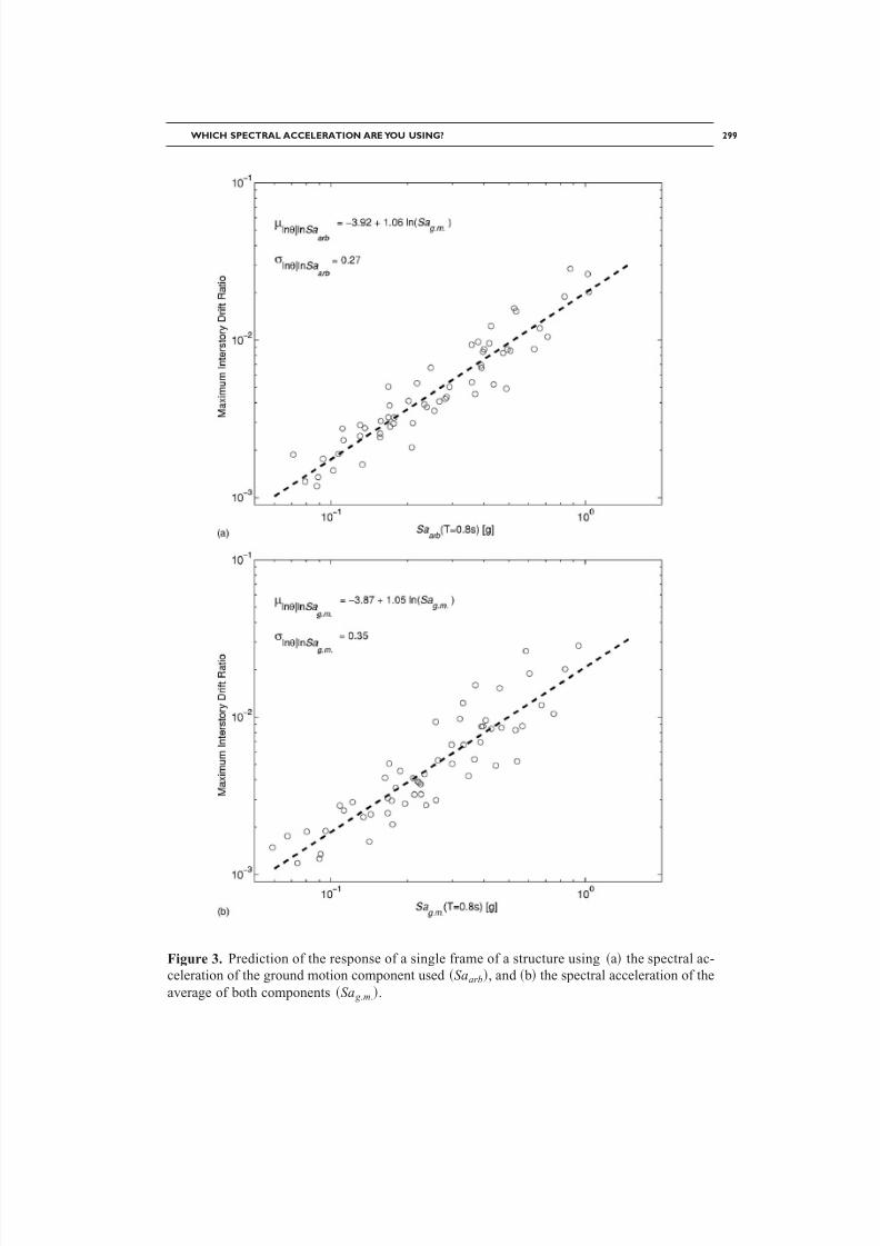
This increased scatter resulting from prediction with Sa g .m. is illustrated in Figure 3.

Prediction of response of a structure is made using both Saarb and Sa g .m.. A model of anolder seven-story reinforced concrete frame, described by Jalayer 2003, is used for

analysis. Sixty unscaled recorded ground motions were used to perform nonlinear dy-namic analysis. Figure 3 shows that the prediction of the mean log maximum interstory

drift ratio, denoted as ln , is very similar for both intensity measures, but use of Sa g .m.

as the IM results in increased dispersion of relative to the use of Saarb, as was antici- pated above. The larger dispersion implies that there is greater uncertainty in the esti-

mate of median response i.e., if Sa g .m. is used as the IM, a greater number of analyses

would need to be performed to achieve the same confidence in the mean ln . Thus the

use of Saarb as the IM is preferable for the structural engineer in order to minimize thenumber of nonlinear dynamic analyses performed.

Many examples of the use of Sa as an intensity measure exist in the literature. For example, modal analysis Chopra 2001, the SAC/FEMA methodology SAC 2000a, b,

c, and incremental dynamic analysis Vamvatsikos and Cornell 2002 all use Sa as a

predictor of structural response in some cases. In virtually every application of these procedures, Saarb as opposed to Sa g .m. is used as the intensity measure for analysis of a single frame of a structure.




Figure 3. Prediction of the response of a single frame of a structure using a the spectral ac-

celeration of the ground motion component used Saarb, and b the spectral acceleration of the

average of both components Sa g .m..




INCORRECT INTEGRATION OF HAZARD AND RESPONSE

Spectral acceleration hazard is coupled with response analysis during performance- based analysis procedures e.g., Cornell and Krawinkler 2000, Cornell et al. 2002. In past application of these procedures, frequently the ground motion hazard analysis has

been unwittingly performed with Sa g .m. to utilize existing attenuation models, and the

response analysis has performed with Saarb to minimize dispersion in the response pre-diction, resulting in the inconsistency discussed in this paper. Examples where the au-

thors know only too intimately that a hazard analysis based on Sa g .m. was inadvertently

coupled with a response analysis based on Saarb include Baker and Cornell 2004, Ja-layer and Cornell 2003, Yun et al. 2002, and Shome and Cornell 1999. In the work of others it is seldom clear because the question was not discussed, but it can be sus-

pected that if the hazard analysis were based on the USGS hazard maps or popular at-tenuation laws such as Abrahamson and Silva 1997 and Sadigh et al. 1997, where the

only reported dispersion is that for Sa g .m., then an inconsistency is likely to exist.

In addition, other design and analysis procedures e.g., ASCE 2000, 2002, utilizethe U.S. Geological Survey maps of spectral acceleration hazard Frankel et al. 2002 to

attain target Sa values at which the performance of the structure should be checked. Al-

though in this case there is no explicit statement of the reliability of a structure analyzed

in this manner, Sa is still used as a link between hazard and response. Thus it is prefer-

able to define Sa consistently in both the hazard and response. Possibilities for a con-sistent treatment of the problem are discussed in the following section.

VALID METHODS OF COMBINING HAZARD AND RESPONSE

For performance-based analysis procedures, it is necessary that the median and dispersion of response at a given IM level be consistent with the IM definition used for

hazard analysis. This can be achieved in several ways, the choice of which may depend in part on the situation and available information. Three proposed solutions for use inanalyzing a structure along a single axis are outlined below. The common characteristicof each method is that the IM used for hazard analysis and the IM used for responseanalysis are consistently defined.

1. CALCULATE THE GROUND MOTION HAZARD FOR Saarb

With this method, the structural response analysis described above is unchanged, but

the ground motion hazard analysis is performed for the consistent intensity measure,Saarb. This allows for the estimation of structural response with less dispersion than

when Sa g .m. is used e.g., see Figure 3. And once more attenuation models are devel-

oped with dispersion for Saarb, the hazard analysis is no more difficult than hazard

analysis for Sa g .m.. The disadvantage is that few current attenuation models provide thedispersion for Saarb, meaning that many models, and the resulting hazard analysis, can-not be used without modification.




2. PREDICT STRUCTURAL RESPONSE USING Sa g .m.

With this method, the ground motion hazard is unchanged from current Sa g .m.-based

practice. Instead, the response analysis is modified, using Sa g .m. as the IM rather thanSaarb. To do this, one would compute the IM of a record as the geometric mean of Sa of

the two components of the ground motion, even though only one component will beused for analysis. This method has the advantage of not requiring new attenuation lawsor hazard analysis. Unfortunately, it will introduce additional dispersion into the re-sponse prediction, as was seen in Figure 3, and hence will be less efficient as an IM.

3. PERFORM HAZARDANALYSISWITH Sa g .m., RESPONSE ANALYSISWITH Saarb,

AND INFLATE THE RESPONSE DISPERSION

This method takes advantage of the fact that the median structural response for a

given Sa level is the same whether Sa g .m. or Saarb is used. Only the dispersion is in-

creased if Sa g .m. is used, as was seen in Figure 3. Structural response is thus performed

using Saarb as per standard practice to obtain the median response. Then the dispersionin response is inflated to reflect that which would have been seen if Sa g .m. had been used as the intensity measure instead. An estimate of the amount by which the dispersionshould be increased can be obtained using a first-order approximation. For this proce-

dure, we assume the following model for the relationship between spectral accelerationand response:

ln = a + b ln Saarb + arb 1

ln = a + b ln Sa g .m. + g .m. 2

where is the structural response value of interest, a and b are coefficients to be esti-

mated from the data using least-squares regression, and ’s are zero-mean random vari-

ables note that a and b have the same expected value in Equations 1 and 2, as is dem-onstrated in the Appendix—Equations 3 and 11—and as is supported by the empiricalestimates in Figure 3. The model is seen to fit well in Figure 3, as in many other cases

at least locally. We are interested in estimating the standard deviation of ln given

Sa g .m., in the case where we know only the standard deviation of ln given ln Saarb.From Equation 13, we can find the ratio of the two conditional standard deviations. For

the example data set here, ln Sa x,ln Sa y=0.797 and ln x,ln Sa x

=0.942, implying a ratio be-

tween standard deviations of 1.34. Thus the predicted conditional standard deviation for

the example problem would be 1.34*0.27=0.36, approximately matching the standard deviation in 2b 0.35.

The SAC procedure SAC 2000a, b, c uses the model of structural response adopted

in Equation 1, but with b = 1. So an analysis using the SAC procedure would be a natural

candidate for this method. One would simply perform analysis using Saarb as before, butinflate the dispersion in structural response using Equation 13 before continuing with theSAC methodology.

In the short term, this third method is attractive because it leaves existing hazard and response procedures unmodified, and instead makes a correction before the two analyses




are combined. However, in the long term one of the two more direct methods using aconsistent IM for both hazard and response would be more expeditious.

RESULTS FROM THE PROPOSED METHODS

All three of the methods described should result in the same answer for the prob-ability of exceedance of a given limit state in the structure, aside from the inherent vari-ability in the answer resulting from the statistically uncertain estimates of hazard and response Baker and Cornell 2003. Additional methods can also be conceived using al-

ternative intensity measures, but the above methods are expected to be the simplest and most similar to current practices.

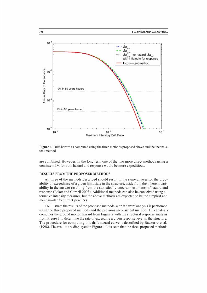
To illustrate the results of the proposed methods, a drift hazard analysis is performed using the three proposed methods and the previous inconsistent method. This analysiscombines the ground motion hazard from Figure 2 with the structural response analysisfrom Figure 3 to determine the rate of exceeding a given response level in the structure.

The procedure for computing this drift hazard curve is described by Bazzurro et al.1998. The results are displayed in Figure 4. It is seen that the three proposed methods

Figure 4. Drift hazard as computed using the three methods proposed above and the inconsis-

tent method.




produce comparable results, while the inconsistent method results are unconservativee.g., the drift level exceeded with a 2% probability in 50 years is underestimated by

approximately 10%. While the magnitude of the error is not overwhelmingly large, itnonetheless represents an easily correctible systematic flaw in the procedure.

In many applications today, the drift hazard curve is not computed. Rather, theground motion hazard is used to specify a target spectral acceleration to use in analyzing

structural response i.e., the spectral acceleration associated with a 2% probability of ex-ceedance in 50 years. An inconsistent approach will cause a comparable bias in thesecalculations as well.

ANALYSIS OF 3-D STRUCTURAL MODELS: COMBINING HAZARD AND

RESPONSE

When analyzing a 3-D structural model, both horizontal components of the ground motion are used, so the above procedures using a single component are not necessarilyapplicable. In this case, as before, the concern is that the intensity measures used in thehazard analysis and response analysis should be consistent. Fortunately, the preferred

method for analysis in this case is also a method that is apparently often used in practice.Several potential procedures are discussed here:

1. USE Sa g .m. AS THE INTENSITY MEASURE

In this case, ground motion hazard analysis is performed for Sa g .m., as is standard

practice today. The intensity measure used for structural response is also Sa g .m., computed for the two components of ground motion used in the analysis. This method is in

use today e.g., Stewart et al. 2001 and appears to be the most straightforward for 3-Dstructures. For this reason, it is currently recommended by the authors when a scalar intensity measure is used see below. The preferred choice of an IM in the case wherethe two axes of the structure have different fundamental periods has not been extensively

examined. In the absence of further research, one obvious possibility is to use Sa g .m. at

an intermediate period e.g., the geometric mean of the two periods.

2. USE Saarb AS THE INTENSITY MEASURE

When using Saarb as an intensity measure in this case, it is necessary to specify thecomponent of the ground motion being measured, as there are now two horizontal com-

ponents used in the analysis, each with a differing value of Sa. If the objective is only ascalar drift hazard curve e.g., there is only a single response parameter of interest, thenthe practitioner may obtain the most efficient estimate by performing the regression

analysis shown in Figure 3 one time for each candidate IM e.g., for Saarb oriented along

the “ x- x” axis of the structure, for Saarb oriented along the “ y- y” axis of the structure,

and for Sa g .m.. Because all three IM choices should lead to the same answer in the limitwith a very large sample of dynamic analyses, the engineer is free to choose the IM thatresults in the most efficient estimation. That is, the IM that results in the smallest stan-dard deviation of response prediction. In some cases, the optimal IM will be apparent

a priori: if the response parameter of interest is a drift in the x- x axis, then it is likely that




the optimal IM is Saarb oriented along the x- x axis. In other cases, for example, whenassessing the axial force in a corner-column of a structure or when there is significant

torsion in the structure, the optimal IM may be less obvious.

In some cases it is necessary to select a common IM for estimation of more than oneresponse parameter simultaneously. For example, in loss estimation procedures associ-ated with performance-based engineering it is often desirable to know the probability

distribution of a set of story drifts and floor accelerations simultaneously. In this case, itmay again be useful to consider several candidate IMs and examine the trade-offs in ef-

ficiency. For instance, Saarb oriented along the x-x axis is likely to estimate the responsesalong the x-x axis efficiently but the responses along the y-y axis less efficiently and vice

versa for Saarb along the y-y axis. Choosing an IM in this case will depend upon therelative importance of the various response parameters of interest, and an understandingof which IM is most efficient for predicting the important response parameters. Note thatthe results for the less-important response parameters will not be incorrect, but only es-

timated with less statistical precision.

The above procedure appears to be valid in the case where no record-scaling is used as part of the response predictions. If the records are scaled before performing the struc-

tural analysis, the scaling procedure must be carefully considered. Previous studies of the implications of scaling a single component of ground motion may not be applicableto scaling of two components. The authors are particularly concerned about the choice of a scale factor for the orthogonal component of a ground motion when a selected com-

ponent has been scaled by a specified factor. This problem is currently under investiga-

tion.

3. USE A VECTOR INTENSITY MEASURE REPRESENTING THE TWO

COMPONENTS INDIVIDUALLY

This approach uses a two-parameter intensity measure, consisting of the spectral ac-celerations in both the x-x and y-y directions. Vector-valued ground motion hazard analy-

sis Bazzurro and Cornell 2002 is used to compute the joint hazard for the spectral ac-celeration values of the two components of ground motion. Response prediction canthen be an explicit function of the two components independently. This approach should reduce the dispersion in structural response and may be useful in some situations e.g.,

the two axes of the structure have differing periods, or Saarb along a given axis is noteffective at estimating responses along the opposite axis. However, this method is notready for widespread adoption until use of vector ground motion hazard analysis be-comes more common.

APPLICATION TO CURRENT PRACTICE

The approaches described above rationally combine the uncertainty in both ground motion hazard and structural response, but they differ from current U.S. building code–

based design practice i.e., ASCE 2002. When dynamic time-history analyses are uti-lized in practice today, a suite of ground motions typically three or seven is scaled to a

target response spectrum obtained using the deterministic or probabilistic hazard analy-sis methods described above. These motions are then used to analyze a structure, and




evaluation is based on either the maximum structural response if fewer than seven mo-tions are used or the average response if at least seven motions are used . But again,

the definition of spectral acceleration is not stated explicitly. An inconsistent basis e.g.,Sa g .m. spectra and Saarb scaling is to be discouraged. As shown above, the use of Sa g .m.

for two-dimensional analysis will result in lower target spectra than when Saarb is used, but higher variation among the structural response. If fewer than seven records are used,then the higher variation of structural response values will be implicitly but not accu-rately captured by the current rule because the maximum response value is likely to belarger. If, however, seven records are used and the average structural response is taken,

then there is no penalty paid for the higher variation of structural response that results

from using Sa g .m. rather than Saarb. Therefore, consistent use of Sa g .m. would be some-what unconservatively biased with seven or more records under the current rule. Theideal solution to this inconsistency would be to incorporate the structural response un-certainty explicitly as is done explicitly in, e.g., SAC 2000a, b, c and Banon et al.

2001. Short of this, the code should require that target response spectrum be based onSaarb when at least seven records are used for two-dimensional analysis, so that theanalysis will include the extra variability in the ground motion intensity. In this casestructural engineers should explicitly request that the hazard analysis and the scaled

ground motion records be based on the Saarb definition of Sa. For three-dimensional

analysis, Sa g .m. is probably the natural choice for the reasons outlined in the previoussection.

CONCLUSIONS

Although intensity measure–based analysis procedures have proven to be usefulmethods for linking the analyses of earth scientists and structural engineers, care isneeded to make sure that the link does not introduce errors into the analysis. Two defi-

nitions of “spectral acceleration” are commonly used by analysts, and the distinction be-tween the definitions is not always made clear. Because of this, a systematic error has

been introduced into the results from many risk analyses, typically resulting in uncon-servative conclusions. For an example site and structure located in Los Angeles, the er-ror resulted in a 12% underestimation of the spectral acceleration value exceeded with a2% probability in 50 years, and a 10% underestimation of the structure’s maximum in-terstory drift ratio exceeded with a 2% probability in 50 years.

This problem is, however, merely one of communication, and not a fundamental flawwith the intensity measure approach. It is not difficult to use intensity measures in waysthat produce correct results. For analysis of a single frame of a structure, the authors see

three paths to the correct answer: 1 use Saarb for both parts of the analysis; 2 use

Sa g .m. for both parts of the analysis; and 3 perform hazard analysis with Sa g .m., and

structural response analysis with Saarb, but inflate the dispersion in the structural re-sponse prediction to represent the dispersion that would have been seen if Sa g .m. had

been used. If a three-dimensional model of a structure is to be analyzed, the most

straightforward method is to use Sa g .m. as the intensity measure for both the ground mo-tion hazard and the structural response. In the absence of a single standard procedure,




both earth scientists and structural analysts are encouraged to explicitly state which Sadefinition they are using for evaluation, in the interest of transparency.

The methods described above will all produce valid estimates of the annual fre-quency of exceeding a given structural response level. In the future it would be desirable

to have attenuation models that estimate the dispersion of both Sa g .m. and Saarb, in order to allow flexibility in the definition of the spectral acceleration used for analysis. Finally,vector-based methods of hazard and response analysis should improve upon the currentsituation in the future.

ACKNOWLEDGMENTS

This work was supported primarily by the Earthquake Engineering Research CentersProgram of the National Science Foundation, under Award Number EEC-9701568through the Pacific Earthquake Engineering Research Center PEER . Any opinions,

findings, and conclusions or recommendations expressed in this material are those of theauthors and do not necessarily reflect those of the National Science Foundation.

APPENDIX: SLOPES AND STANDARD DEVIATIONS OF

REGRESSION PREDICTIONS

This appendix explores in more detail the prediction of structural response as a func-tion of either spectral acceleration of an arbitrary component or an average component.

Consider a set of earthquake ground motions consisting of two components. We will re-fer to these two components as the “X” and “Y” components for clarity the commonassumption of no preferential orientation of motion is made here, which is typicallyvalid when near-fault directivity effects are not present. Now consider the probabilisticdistribution of the spectral acceleration values of these ground motion components.

Logarithms of spectral acceleration and structural response are used, to take advantageof the linear relationships in the logarithmic domain often observed between these vari-ables e.g., Figure 3 and 5.

The ln Sa values of the x and y components have means, denoted as µln Sa xand µln Sa y

,

and standard deviations, denoted as ln Sa xand ln Sa y

. Because there is no preferential

direction to these motions, µln Sa x= µln Sa y

and ln Sa x= ln Sa y

although our estimates of

these values for a particular data set might not be exactly equal, the underlying true val-ues are assumed to be. We can compute a correlation coefficient between the two com-

ponents, denoted as ln Sa x,ln Sa y. The dependence between ln Sa x and ln Sa y is purely lin-

ear due to the lack of preferential orientation, as can be seen, for example, in Figure 5.

We make the further mild assumption that the conditional variances of ln Sa y givenln Sa x and ln Sa x given ln Sa y are constant.

Consider now the analysis of a structural frame, oriented along the x axis of theground motions. We perform nonlinear dynamic analysis with the x component of eachground motion to calculate a set of structural response values. The logarithmic response

values have a mean, µln x, and a standard deviation, ln x

. There is a relationship be-

tween ln Sa x log spectral acceleration in the x direction and ln x log response of the

structure, oriented in the x direction that can be represented by a linear correlation, and




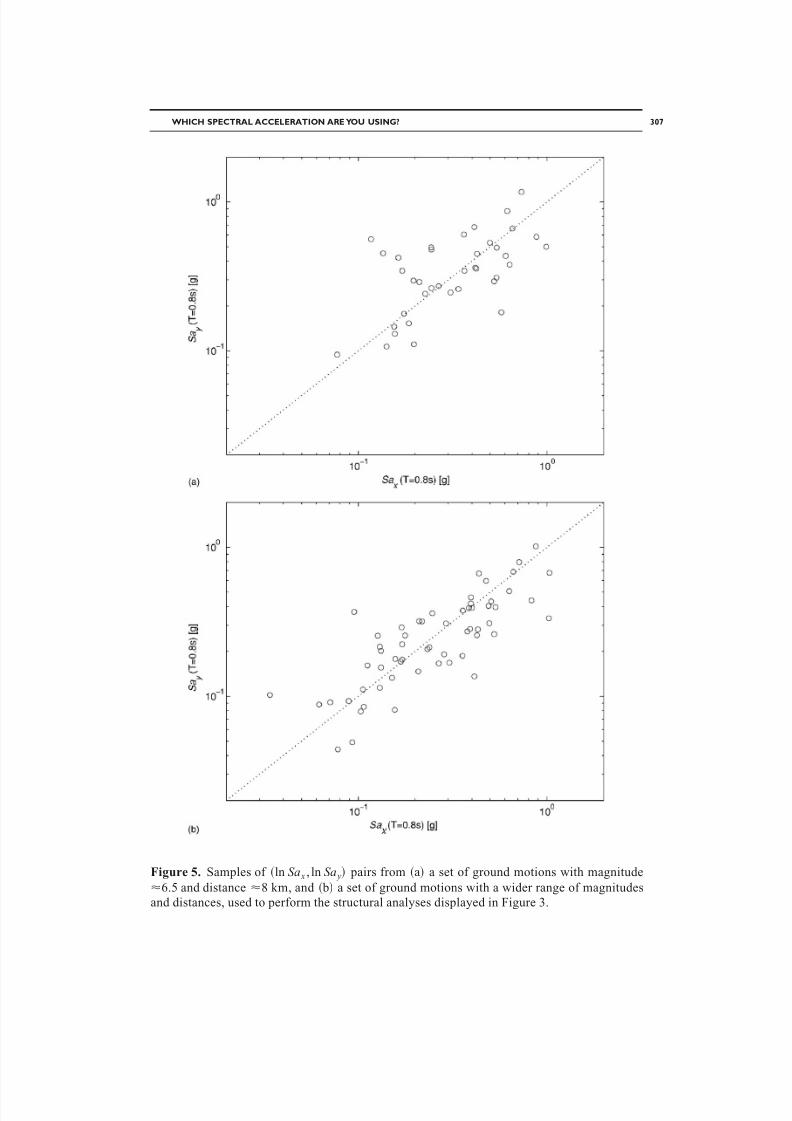
Figure 5. Samples of ln Sa x , ln Sa y pairs from a a set of ground motions with magnitude

6.5 and distance 8 km, and b a set of ground motions with a wider range of magnitudes

and distances, used to perform the structural analyses displayed in Figure 3.




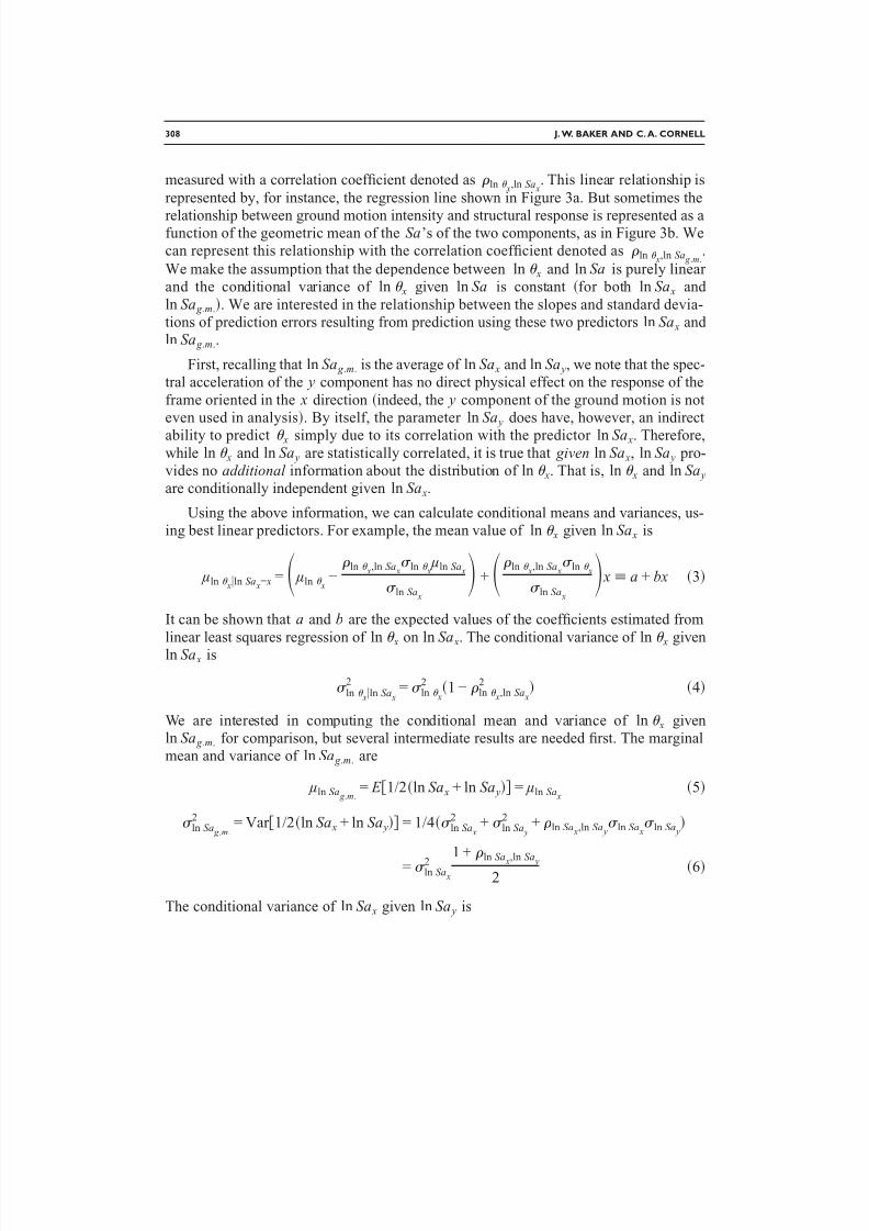
measured with a correlation coefficient denoted as ln x,ln Sa x. This linear relationship is

represented by, for instance, the regression line shown in Figure 3a. But sometimes the

relationship between ground motion intensity and structural response is represented as afunction of the geometric mean of the Sa’s of the two components, as in Figure 3b. We

can represent this relationship with the correlation coefficient denoted as ln x,ln Sa g .m..

We make the assumption that the dependence between ln x and ln Sa is purely linear

and the conditional variance of ln x given ln Sa is constant for both ln Sa x and

ln Sa g .m.. We are interested in the relationship between the slopes and standard devia-

tions of prediction errors resulting from prediction using these two predictors ln Sa x and ln Sa g .m..

First, recalling that ln Sa g .m. is the average of ln Sa x and ln Sa y, we note that the spec-

tral acceleration of the y component has no direct physical effect on the response of the

frame oriented in the x direction indeed, the y component of the ground motion is not

even used in analysis. By itself, the parameter ln Sa y does have, however, an indirect

ability to predict x simply due to its correlation with the predictor ln Sa x. Therefore,while ln x and ln Sa y are statistically correlated, it is true that given ln Sa x, ln Sa y pro-

vides no additional information about the distribution of ln x. That is, ln x and ln Sa y

are conditionally independent given ln Sa x.

Using the above information, we can calculate conditional means and variances, us-

ing best linear predictors. For example, the mean value of ln x given ln Sa x is

µln xln Sa x= x = µln x−

ln x,ln Sa x ln x

µln Sa x

ln Sa x

+ ln x,ln Sa x ln x

ln Sa x

x a + bx 3

It can be shown that a and b are the expected values of the coefficients estimated from

linear least squares regression of ln x

on ln Sa x

. The conditional variance of ln x

givenln Sa x is

ln xln Sa x

2= ln x

2 1 − ln x,ln Sa x

2 4

We are interested in computing the conditional mean and variance of ln x givenln Sa g .m. for comparison, but several intermediate results are needed first. The marginal

mean and variance of ln Sa g .m. are

µln Sa g .m.= E 1/2ln Sa x + ln Sa y = µln Sa x

5

ln Sa g .m.

2 = Var 1/2ln Sa x + ln Sa y = 1/4 ln Sa x

2 + ln Sa y

2 + ln Sa x,ln Sa y ln Sa x

ln Sa y

= ln Sa x2

1 + ln Sa x

,ln Sa y

2 6

The conditional variance of ln Sa x given ln Sa y is




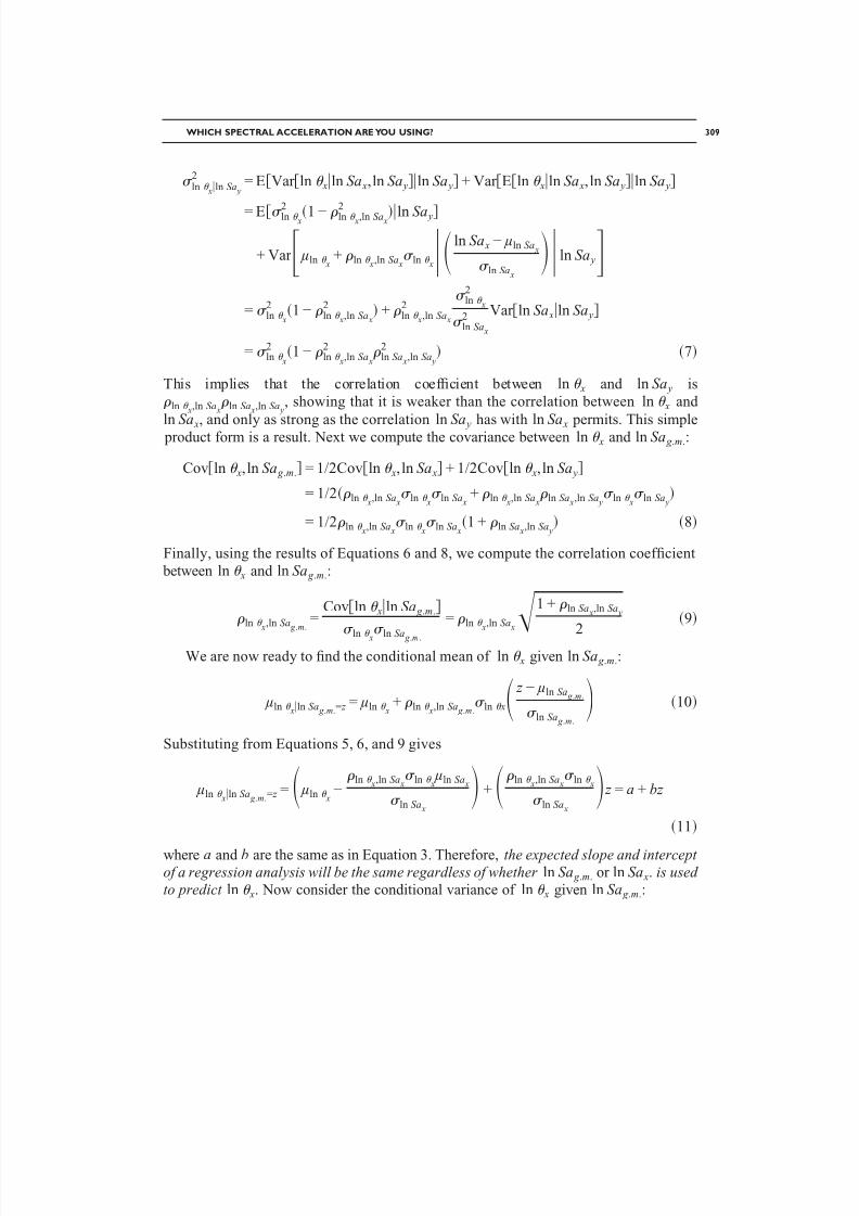
ln xln Sa y

2 = EVar ln xln Sa x,ln Sa yln Sa y + Var Eln xln Sa x, ln Sa yln Sa y

= E ln x

2

1 − ln x,ln Sa x

2

ln Sa y

+ Var µln x+ ln x,ln Sa x

ln x ln Sa x − µln Sa x

ln Sa x

ln Sa y= ln x


2 + ln x,ln Sa x

2 ln x

2

ln Sa x

2 Var ln Sa xln Sa y

= ln x


2 ln Sa x,ln Sa y

2 7

This implies that the correlation coefficient between ln x and ln Sa y is

ln x,ln Sa x ln Sa x,ln Sa y

, showing that it is weaker than the correlation between ln x and

ln Sa x, and only as strong as the correlation ln Sa y has with ln Sa x permits. This simple product form is a result. Next we compute the covariance between ln x and ln Sa g .m.:

Covln x, ln Sa g .m. = 1/2Covln x, ln Sa x + 1/2Covln x, ln Sa y

= 1/2 ln x,ln Sa x ln x

ln Sa x+ ln x,ln Sa x

ln Sa x,ln Sa y ln x

ln Sa y

= 1/2 ln x,ln Sa x ln x

ln Sa x1 + ln Sa x,ln Sa y

8

Finally, using the results of Equations 6 and 8, we compute the correlation coefficient

between ln x and ln Sa g .m.:

ln x,ln Sa g .m.=

Covln xln Sa g .m.

ln

x

ln Sa g .m.

= ln x,ln Sa x1 + ln Sa x,ln Sa y

29

We are now ready to find the conditional mean of ln x given ln Sa g .m.:

µln xln Sa g .m.= z = µln x+ ln x,ln Sa g .m.

ln x z − µln Sa g .m.

ln Sa g .m.

10

Substituting from Equations 5, 6, and 9 gives

µln xln Sa g .m.= z = µln x−

ln x,ln Sa x ln x

µln Sa x

ln Sa x

+ ln x,ln Sa x ln x

ln Sa x

z = a + bz

11

where a and b are the same as in Equation 3. Therefore, the expected slope and intercept of a regression analysis will be the same regardless of whether ln Sa g .m. or ln Sa x. is used

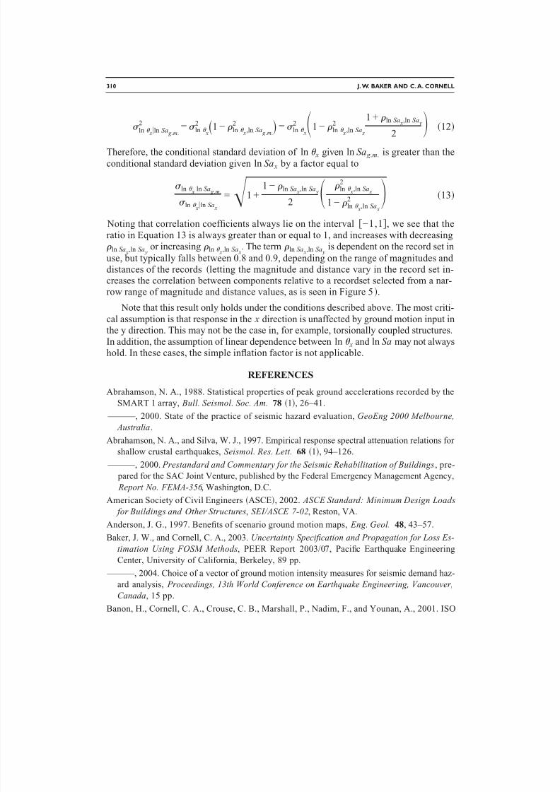
to predict ln x. Now consider the conditional variance of ln x given ln Sa g .m.:




ln xln Sa g .m.

2 = ln x

2 1 − ln x,ln Sa g .m.

2 = ln x


21 + ln Sa x,ln Sa y

2

12

Therefore, the conditional standard deviation of ln x given ln Sa g .m. is greater than the

conditional standard deviation given ln Sa x by a factor equal to

ln xln Sa g .m.

ln xln Sa x

=1 +1 − ln Sa x,ln Sa y

2 ln x,ln Sa x

2

1 − ln x,ln Sa x

2 13

Noting that correlation coefficients always lie on the interval −1,1, we see that the

ratio in Equation 13 is always greater than or equal to 1, and increases with decreasing ln Sa x,ln Sa y

or increasing ln x,ln Sa x. The term ln Sa x,ln Sa y

is dependent on the record set in

use, but typically falls between 0.8 and 0.9, depending on the range of magnitudes and distances of the records letting the magnitude and distance vary in the record set in-

creases the correlation between components relative to a recordset selected from a nar-row range of magnitude and distance values, as is seen in Figure 5.

Note that this result only holds under the conditions described above. The most criti-

cal assumption is that response in the x direction is unaffected by ground motion input inthe y direction. This may not be the case in, for example, torsionally coupled structures.

In addition, the assumption of linear dependence between ln x and ln Sa may not alwayshold. In these cases, the simple inflation factor is not applicable.

REFERENCES

Abrahamson, N. A., 1988. Statistical properties of peak ground accelerations recorded by the

SMART 1 array, Bull. Seismol. Soc. Am. 78 1, 26–41.

———, 2000. State of the practice of seismic hazard evaluation, GeoEng 2000 Melbourne, Australia.

Abrahamson, N. A., and Silva, W. J., 1997. Empirical response spectral attenuation relations for

shallow crustal earthquakes, Seismol. Res. Lett. 68 1, 94–126.

———, 2000. Prestandard and Commentary for the Seismic Rehabilitation of Buildings, pre-

pared for the SAC Joint Venture, published by the Federal Emergency Management Agency,

Report No. FEMA-356 , Washington, D.C.

American Society of Civil Engineers ASCE, 2002. ASCE Standard: Minimum Design Loads

for Buildings and Other Structures, SEI/ASCE 7-02, Reston, VA.

Anderson, J. G., 1997. Benefits of scenario ground motion maps, Eng. Geol. 48, 43–57.

Baker, J. W., and Cornell, C. A., 2003. Uncertainty Specification and Propagation for Loss Es-

timation Using FOSM Methods, PEER Report 2003/07, Pacific Earthquake Engineering

Center, University of California, Berkeley, 89 pp.

———, 2004. Choice of a vector of ground motion intensity measures for seismic demand haz-

ard analysis, Proceedings, 13th World Conference on Earthquake Engineering, Vancouver,

Canada, 15 pp.

Banon, H., Cornell, C. A., Crouse, C. B., Marshall, P., Nadim, F., and Younan, A., 2001. ISO




ings, prepared for the Federal Emergency Management Agency, Report No. FEMA-350,

Washington, D.C.

———, 2000c. Recommended Seismic Evaluation and Upgrade Criteria for Existing Welded Steel Moment-Frame Buildings, prepared for the Federal Emergency Management Agency,

Report No. FEMA-351, Washington, D.C.

Sadigh, K., Chang, C.-Y., Egan, J. A., Makdisi, F., and Youngs, R. R., 1997. Attenuation rela-

tionships for shallow crustal earthquakes based on California strong motion data, Seismol.

Res. Lett. 68 1, 180–189.

Shome, N., and Cornell, C. A., 1999. Probabilistic Seismic Demand Analysis of Nonlinear

Structures, RMS Program, RMS-35, Stanford, CA, 320 pp. http://www.stanford.edu/group/

rms/accessed 3/14/05.

Spudich, P., Joyner, W. B., Lindh, A. G., Boore, D. M., Margaris, B. M., and Fletcher, J. B.,

1999. SEA99: A revised ground motion prediction relation for use in extensional tectonic

regimes, Bull. Seismol. Soc. Am. 89 5, 1156–1170.

Stewart, J. P., Chiou, S.-J., Bray, J. D., Graves, R. W., Somerville, P. G., and Abrahamson, N. A.,

2001. Ground Motion Evaluation Procedures for Performance-Based Design, PEER Report

2001/09, Pacific Earthquake Engineering Center, University of California, Berkeley, 229 pp.

Vamvatsikos, D., and Cornell, C. A., 2002. Incremental dynamic analysis, Earthquake Eng.

Struct. Dyn. 31 3, 491–514.

Yun, S.-Y., Hamburger, R. O., Cornell, C. A., and Foutch, D. A., 2002. Seismic performance

evaluation for steel moment frames, J. Struct. Eng. 128 4, 12.

Received 21 February 2005; accepted 26 July 2005


which sa are you using-baker

Documents