which transient when? - a utility function for transient follow-up scheduling

Which transient, when?A utility function for transient follow-up scheduling

Tim Staley(4 Pi Sky group)

Southampton Wednesday Seminar, May 2015

WWW: 4pisky.org , timstaley.co.uk/talks

4pisky.org

timstaley.co.uk/talks

Automate all the things Forecasting transients Decision theory Future work

Outline

Automate all the things

Forecasting transients

Decision theory

Future work


LSST predicted transient rates

(LSST science book, 2009)

Orphan GRBS: ∼ 1000 per year.

“The reader should be cautioned that many of theserates are very rough.”

Guesstimates: 104 – 106 alerts per night(depending on your definition).


Transient rates today

Notices / events in a 30 day period around April 2015:

É GCN: 106 (perhaps 10 new events)

É ATEL: 146 (probably similar ratio of new / follow-up)

É GAIA: 17 (public)

É PTF: 299 (internal)

É CRTS: 81(CSS) + 105 (MLS) (automatic detections)

Just counting initial events: ∼500 / month, or ∼17 /day


Robotic follow-up facilitiesSlow rise of automated sites / networks, e.g.LCOGT: 2 × 2m + 9 × 1m telescopes, over six sites.

(http://lcogt.net/observatory)

http://lcogt.net/observatory


The (wider) problem

How do we begin to ‘close the loop’ ofobserve =⇒ analyse =⇒ observe?


The (wider) problem


Transient discovery

Observation prioritization

Classification estimates

Interesting?

Yes

Schedule optimization

External alerts

Survey data

Telescope agents

Follow-up data


The (wider) problem


Transient discovery



Interesting?

Yes


External alerts

Survey data

Telescope agents

Follow-up data

Science!


Diversion on DG-CVn superflare

Fender 2014, http://adsabs.harvard.edu/abs/2014arXiv1410.1545F

Osten et al (in prep)

http://adsabs.harvard.edu/abs/2014arXiv1410.1545F


Missing pieces

Transient discovery



Interesting?

Yes


External alerts

Survey data

Telescope agents

Follow-up data

É We’ve found a potentially interesting new transient.

É Looks like it could be one of class A, B, or C.

É What now?


We found a transient!What now?

Two implicit goals of follow-up observation:

É Improving classification(Let’s see if it’s really class A.)

É Further observation(Tell me more! / Boring!)

. . . I’ll mainly be talking about the former.


Outline



Decision theory

Future work


Working with tiny dataWe’ve found a transient. But, very few datapoints:

−10 −5 0 5 10 15 20 25 30Time

0

2

4

6

8

10

12

Flu

x

Detection thresholdData


The set-up

How do we predict the possible futures for a giventransient?

For now, make some simplifying assumptions:

É Parametric lightcurve models for each class oftransient.

É Each transient class has a known prior distributionover the morphological parameters, and this ismultivariate Normal.


Assumption: Parametric models

Deterministic, finite number of parameters e.g.

y = ƒ (t, t0, , τrse, τdecy)

−40 −20 0 20 40 60 80 100Time

0

2

4

6

8

10

Flu

x


Result: Line of best fit

(Maximum likelihood)

−10 −5 0 5 10 15 20 25 30Time

0

2

4

6

8

10

12

Flu

x

ML fitDetection thresholdData


Assumption: Multivar-Normal priors

Known priors, normally distributed, covariant

2

3

4

rise_

tau

8 16 24 32

a

6

12

18

24

deca

y_ta

u

2 3 4

rise_tau

6 12 18 24

decay_tau


Construct: Model lightcurve ensembles

−20 0 20 40 60 80Time

0

2

4

6

8

10

12

14

16

18

Flu

x


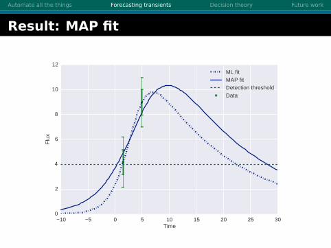
Result: MAP fit

−10 −5 0 5 10 15 20 25 30Time

0

2

4

6

8

10

12

Flu

x

ML fitMAP fitDetection thresholdData


But...

−10 −5 0 5 10 15 20 25 30Time

0

2

4

6

8

10

12

Flu

x

ML fitMAP fitTrueDetection thresholdData


Constrained parameter distributions

Take our two datapoints, run some MCMC fitting...

3.0

3.6

4.2

rise_

tau

12151821

deca

y_ta

u

10 15 20 25 30

a

0

4

8

12

t0

3.0 3.6 4.2

rise_tau12 15 18 21

decay_tau

0 4 8 12

t0


Constrained lightcurve ensembles

−30 −20 −10 0 10 20 30 40 50Time

0

2

4

6

8

10

12

14

16

18

Flu

x

TrueObservations

Comparison, 2 datapoints



−30 −20 −10 0 10 20 30 40 50Time

0

5

10

15

Flu

x

TrueForecast epochObservations

0.00 0.05 0.10 0.15Prob.

0

5

10

15




−30 −20 −10 0 10 20 30 40 50Time

0

2

4

6

8

10

12

14

16

Flu

x


0.0 0.2 0.4 0.6Prob.

0

2

4

6

8

10

12

14

16




−30 −20 −10 0 10 20 30 40 50Time

0

5

10

15

Flu

x


0.00 0.05 0.10 0.15Prob.

0

5

10

15




−30 −20 −10 0 10 20 30 40 50Time

0

2

4

6

8

10

12

Flu

x


0.0 0.2 0.4 0.6Prob.

0

2

4

6

8

10

12




−30 −20 −10 0 10 20 30 40 50Time

0

2

4

6

8

10

12

Flu

x


0.00 0.25 0.50 0.75Prob.

0

2

4

6

8

10

12



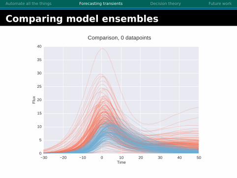
Comparing model ensembles

−30 −20 −10 0 10 20 30 40 50Time

0

2

4

6

8

10

12

14

16

18

Flu

xPrior ensemble, Type 1



−30 −20 −10 0 10 20 30 40 50Time

0

5

10

15

20

25

30

35

Flu

xPrior ensemble, Type 2



−30 −20 −10 0 10 20 30 40 50Time

0

5

10

15

20

25

30

35

40

Flu

xComparison, 0 datapoints



−30 −20 −10 0 10 20 30 40 50Time

0

5

10

15

20

25

30

35

Flu

x


0.00 0.05 0.10 0.15 0.20Prob.

0

5

10

15

20

25

30

35




−30 −20 −10 0 10 20 30 40 50Time

0

5

10

15

20

25

30

35

Flu

x


0.0 0.2 0.4 0.6Prob.

0

5

10

15

20

25

30

35



Outline



Decision theory

Future work


The crux of the problem

(Couldn’t get past thecrux)

É Computers are good atoptimisation.

É e.g., picking out a goodobserving schedule.

É But need a way toassign value.


−6 −4 −2 0 2 4 6Epoch

0.0

0.2

0.4

0.6

0.8

1.0

Rel

ativ

e flu

x

stablelogisticnull

Intrinsic lightcurves


−6 −4 −2 0 2 4 6Epoch

0.0

0.2

0.4

0.6

0.8

1.0

Rela

tive f

lux

stable

logistic

null

Intrinsic LC's with noise estimates


−6 −4 −2 0 2 4 6Epoch

−0.5

0.0

0.5

1.0

1.5

Rel

ativ

e flu

xSampling with noise


0 1−0.5

0.0

0.5

1.0

1.5R

elat

ive

flux

T=-5.0

0 1

T=-4.0

0 1PDF value

T=-3.0

0 1

T=-2.0

0 1

T=-1.0

0 1

T=0.0

0 1

T=1.0

0 1

T=2.0

stablelogisticnull

Class PDF at each epoch


PDF value−0.5

0.0

0.5

1.0

1.5

Rel

ativ

e flu

x

T=-5.0 T=-4.0 T=-3.0 T=-2.0 T=-1.0 T=0.0 T=1.0 T=2.0

stablelogisticnull

−5 −4 −3 −2 −1 0 1 2Epoch

−0.55−0.50−0.45−0.40−0.35−0.30−0.25−0.20

FoM

Information content

Evaluating each epoch


The problem with information content

PDF value−0.5

0.0

0.5

1.0

1.5R

elat

ive

flux

T=-5.0 T=-4.0 T=-3.0 T=-2.0 T=-1.0 T=0.0 T=1.0 T=2.0

stablelogisticnull

−5 −4 −3 −2 −1 0 1 2Epoch

−0.55−0.50−0.45−0.40−0.35−0.30−0.25−0.20

FoM

Information content


Information content weights all classes equally.What if we’re more interested in identifying one

particular class?


Introducing: confusion matrices

Common or garden empirical confusion matrix:

(Automatic classification of time-variable X-ray sources;K. Lo et al, 2014)


Confusion matrices

Label True class

A B C

A P( A | A ) P( A | B ) P( A | C )

B P( B | A ) P( B | B ) P( C | C )

C P( C | A ) P( C | B ) P( C | C )


Probabilistic confusion matricesExample

0.0 0.5 1.0 1.5 2.0 2.5PDF value

−0.5

0.0

0.5

1.0

1.5

Rel

ativ

e flu

x

T=-2

stablelogisticnull

True classstable logistic null

Labelstable 0.549 0.449 0.002logistic 0.449 0.541 0.010null 0.002 0.010 0.988

Diagonal entries representrecall for each class.


PDF value−0.5

0.0

0.5

1.0

1.5

Rel

ativ

e flu

x

T=-5.0 T=-4.0 T=-3.0 T=-2.0 T=-1.0 T=0.0 T=1.0 T=2.0

stablelogisticnull

−5 −4 −3 −2 −1 0 1 2Epoch

0.450.500.550.600.650.700.750.800.850.90

FoM

Information content (shifted)Total Recall



PDF value−0.5

0.0

0.5

1.0

1.5

Rel

ativ

e flu

x

T=-5.0 T=-4.0 T=-3.0 T=-2.0 T=-1.0 T=0.0 T=1.0 T=2.0

stablelogisticnull

−5 −4 −3 −2 −1 0 1 2Epoch

0.50.60.70.80.91.0

FoM

Total RecallNull Recall



As applied to the previous example . . .

−30 −20 −10 0 10 20 30 40 50Time

0

5

10

15

20

25

30

35Flu

x

True

Forecast epoch

Observations

0.00 0.08 0.16 0.24 0.32Prob.

0

5

10

15

20

25

30

35

−30 −20 −10 0 10 20 30 40 50Time

−0.70−0.65−0.60−0.55−0.50−0.45−0.40

IC s

core



Summary

É Data + models + Bayesian analysis =⇒Ensemble forecasts

É Ensemble forecasts + utility function =⇒Figure-of-merit for evaluating possible actions

É Using the figure-of-merit as basis for a decision =Applied Bayesian decision theory(AKA active machine learning)


Outline



Decision theory

Future work


Scheduler, simulation, testing

É Still need to implement a (basic) scheduler usingfigure-of-merit as input.

É Then: simulate (easy, already have models!)


Optimization / Automated Planning

É Optimizing for ASAP classification(Future-discounted weighting schemes?)

É Non-myopic (better-than-greedy) scheduling.

É Multi-armed bandit problem.


Optimization / Automated PlanningMulti-armed bandit problem

Image credit: Wikipedia/Yamaguchi (CC BY-SA 3.0)


Model refinement (and basic validity)

É Multivariate normal prior — valid?

É Sum of multiple multivariate normals?

É Non-parametric modelling (Gaussian processes)?


Culture

Pretty sure we can make this work. . . but there’s aculture / chicken-and-egg problem.


Code packages used

É astropy.modeling — for the models interface.

É Numpy — efficient lightcurve-model calculations.

É pandas — (Python ANalysis of DAta Series) forhandling time-series data.

É statsmodels — Kernel density estimates.

É emcee — for MCMC

É (Py)MultiNest — For model-evidence calculations.

É Seaborn — Neat plotting tools, aestheticallypleasing defaults for Matplotlib.

http://docs.astropy.org/en/stable/modeling/index.html

http://pandas.pydata.org/

http://statsmodels.sourceforge.net/

http://dan.iel.fm/emcee/current/

https://ccpforge.cse.rl.ac.uk/gf/project/multinest/

http://stanford.edu/~mwaskom/software/seaborn/


Fin

Plenty more to do . . . watch this space.