who becomes a politician?

Who Becomes a Politician? ∗

Ernesto Dal Bo, Frederico Finan, Olle Folke,Torsten Persson, and Johanna Rickne

February 2016

Abstract

Can a democracy attract competent leaders, while attaining broad rep-resentation? Economic models suggest that free-riding incentives and loweropportunity costs give the less competent a comparative advantage at enter-ing political life. Also, if elites have more human capital, selecting on com-petence may lead to uneven representation. We examine patterns of politicalselection among the universe of municipal politicians in Sweden using extraor-dinarily rich data on competence traits and social background for the entirepopulation. We document four new facts: First, Politicians are on averagesignificantly smarter and better leaders than the population they represent.Second, the representation of social background, whether measured by inter-generational earnings or social class, is remarkably even. Third, there is at besta weak tradeoff in selection between competence and representation. Fourth,both material and intrinsic motives matter in selection, as does screening bypolitical parties.

∗We are grateful to participants in seminars at CIFAR, UDESA, Berkeley, Bocconi, LSE andLBS for helpful comments and to the Soderberg Foundation and the Swedish Research Council forfinancial support.

1 Introduction

The identity of political leaders affects which policies get selected, how well theyare implemented, and who benefits from them.1 While this is intuitive for autocra-cies where rulers face few constraints, it is also true for representative democracies,because policy platforms do not constitute complete enforceable contracts. Mostvoters would therefore like to elect highly competent policymakers for choosing andimplementing policies to attain a given objective. As a collective, voters may wantto elect policymakers who represent diverse interests, so that government will pursuebroad objectives.

Whether representative democracy can deliver both high-ability leaders and broadrepresentation is unclear. Economic models of politics suggest that the less ablehave a comparative advantage at entering public life due to free-riding incentives(Olson 1965; Messner and Polborn 2004) and lower opportunity costs (Caselli andMorelli 2004). In addition, if ability is distributed unequally in society, selecting oncompetence may make it harder to ensure broad representation. Related to this, anumber of scholars have argued that the electoral system shapes the tradeoff betweenaccountability – a driver of selection – and representation.2

To better understand political selection, and the potential tradeoffs it entails,we need to thoroughly describe selection patterns and analyze their determinants.Unfortunately, insufficient data has made it difficult to carry out these tasks.

Three data limitations First, any study of political selection should accountfor two stages, namely candidate entry and candidate screening by voters and/orparties. The study of candidate screening requires information on both elected andnon-elected politicians. While information on the former is sometimes available,information on the latter is remarkably sparse. A few studies have tried to tackle thisdata limitation to advance our understanding of candidate selection.3 Unfortunatelythis literature misses candidate entry, which requires information on those who didnot even attempt political entry.

Second, much of the relevant theory emphasizes the quality of political selection.

1See for example Pande (2003), Chattopadhyay and Duflo (2004), Jones and Olken (2005),Washington (2008), Besley, Montalvo, and Reynal-Querol (2011), Meyersson (2014).

2A common idea is that plurality rule fosters better accountability, while proportional repre-sentation fosters better representation (Myerson 1993; Persson and Tabellini 2003; Powell 2000;Taagepera and Shugart 2000).

3Examples include: Besley, Pande, and Rao (2005), Ferraz and Finan (2009), Galasso andNannicini (2011), Beath, Christia, Egorov, and Enikolopov (2014), Jia, Kudamatsu, and Seim(2015), and Tillmann (2014).

1

But how to measure quality or competence? Absent direct data on the underlyingintelligence or personality traits of politicians, the existing empirical literature hasrelied on proxies such as education, occupation, or pre-office income levels (Dal Bo,Dal Bo, and Snyder 2009; Ferraz and Finan 2009; Merlo, Galasso, Landi, and Mat-tozzi 2010; Galasso and Nannicini 2011; Besley and Reynal-Querol 2011). Whilecorrelated with competence, these proxies also likely reflect luck or social class.

Third, representation is hard to measure. Previous work has relied on proxies likea politician’s occupation. However, occupation is also coarse: many politicians maybe lawyers, but if values and loyalties depend on social background one would like toknow if they were brought up as elite or working class. This requires intergenerationalinformation that is difficult to obtain.

In sum, we know of no research that has been able to analyze both stages of theselection process, using a comprehensive bundle of traits that accurately reflect theability and representativeness of politicians.

Sweden as a test bed Our study overcomes these limitations by using detailedadministrative data from Sweden. The focus on Sweden deserves some justificationbeyond data availability. Clearly, conclusions based upon evidence from a singlecountry cannot be extrapolated to the rest of the world. But Sweden is of interestfor its commonalities with other countries, as well as for its differences. Swedish poli-tics is based on an electoral party system with proportional representation, the mostcommon type of democracy in the world. Sweden is also a quintessential advanceddemocracy. It has remained stable and fully democratic (scoring a perfect 10 in the−10 to 10 Polity-IV scale) for a long period, during which other states experienceda gradual transition from autocracy to democracy. Sweden thus exemplifies the in-stitutional destination many countries around the world may be approaching. Whendebating the value of democracy it is natural to ask if a democratic transition canimprove the ability and representativeness of leaders. If Sweden displayed incompe-tent and unrepresentative leaders, defenders of democratization may have to resortto different arguments.

Our data The Swedish data allows us to undertake the most thorough descriptionto date of the basic patterns of political selection in a country. A key advantage is theavailability of rich measures of competence and social background. The competencemeasures include evaluations of IQ and leadership potential done by the militaryon the universe of the male population, and a measure of residual ability (for bothgenders) stemming from a fully saturated Mincer regression that was developed byBesley, Folke, Persson, and Rickne (2013). Our social-background data includes

2

reliable intergenerational information, namely social class as reflected in parentaloccupations (a traditional approach in sociology) as well as parental income.

We focus on municipal politicians – who are important providers of public goods– to take advantage of larger numbers and within-country variation. We approachthese data at three different levels of analysis that make for the three main sectionsof the paper.

Aggregate level At the highest aggregate level, we uncover new statistics onpolitical selection for Sweden as a whole. Are politicians positively or negativelyselected in terms of ability? Standard models of occupational choice would predictadverse selection: able prospective politicians have higher pre-office incomes andmore promising careers and hence face higher opportunity costs from entering pub-lic life. Nevertheless, we document strong positive selection along all competencemeasures. Selection monotonically improves from those merely nominated to thoseelected, and from rank-and-file elected council members to mayors. Mayors are al-most as positively selected as national legislators and members of elite occupationsin the private and public sectors.

We then examine the social origin of politicians. While politicians themselves aredisproportionately high-earning individuals, the distributions of their parents’ socialclass as well as parental earnings look almost identical to those of the population. Inother words, politics is not reserved for the scions of rich elite families but tracks theentire social structure. This remarkably even representation is the result of differentpolitical parties representing different segments of the income distribution.

The findings on representation help us understand the drivers of positive selectionon ability. A priori, positive selection could reflect either meritocracy that worksindependently of social class, or elitism that works via privileged access to human-capital (itself manifested in competence measures) cum easier access to politicalpower. If elitism is the main driver of access to political office, family backgroundshould strongly predict selection and, conditional on that background, individualtraits should not. Our findings on representation indicate that family background isnot an important driver. Moreover, when we compare the competence of politiciansand their siblings, we find differences nearly as large as those separating politiciansfrom the general population. This indicates that, conditional on family background,individual traits matter greatly for selection.

Municipal level In the second part, we examine municipal heterogeneity. Here, wetest whether municipalities that display stronger selection on ability do so at the costof narrower representation. We document substantial variation across municipalities

3

in each dimension of selection, but find no evidence of an acute tradeoff. Upon closerinspection, the flat tradeoff reflects stronger selection on competence among lowersocioeconomic strata.

Individual level Finally we consider the decisions of individuals about entry intopolitics, and the role that political parties may play in allowing them access topolitical office. A highly stylized formal model, which shares some features withthe aforementioned economic selection models, guides our thinking on drivers ofself-selection. It predicts that (i) higher mayoral wages attract more competentindividuals not only to the mayor position, but also to engage in politics. Themodel also predicts selection into politics to be improved by (ii) intrinsic motivationfor public service, and (iii) lower returns to seniority in one’s private career. Thecorrelations we find in the data are consistent with these predictions.

Our analysis also indicates that, given self-selection choices, the strong positiveselection on competence likely reflects positive screening by political parties. Partiesmay serve as arenas where the more able are allowed in, and promoted to positionsof influence. This hypothesis matches qualitative work in political science, whichdescribes the active involvement of parties in promoting the more competent. Italso matches two facts in our data, namely that competence increases with list rankswithin parties, and that competence for each list rank increases with levels of politicalcompetition within municipalities.

Organization of the paper In the next section we offer background informationon the Swedish political system. Section 3 describes our data and their sources. InSection 4, we present the aggregate results on political selection of ability and socialorigin. Section 5 explores the two dimensions of selection across municipalities, andexamines the prospective tradeoff between selecting on ability and achieving broadrepresentation. In Section 6, we analyze individual self-selection, both theoreticallyand empirically, and discuss the role of parties as screening devices. We conclude inSection 7.

2 Background

Sweden’s electoral system Sweden has three administrative levels of govern-ment. Every four years (three years prior to 1994), elections are run for 290 munic-ipalities, 20 counties, and the nation. All elections take place on the same day andturnout is between 80 and 90 percent. In each election citizens cast a separate party

4

ballot, a ranked list with a large number of candidates. This system elects a total of349 parliamentarians, 1,100 county-council members, and 13,000 municipal-councilmembers. Our paper focuses on the latter.

In Sweden’s proportional representation system, seat shares in the municipalcouncils are proportional to the vote share of each party. Until 1998, seats for eachparty were handed out from the top of the ballot (so-called closed lists). Since 1998,voters can also cast an optional preference vote for one candidate. But this reformhas only allowed a handful of politicians from lower ranks to bypass the party’s listorder and win a seat.4

Based on the distribution of council seats, a ruling majority is formed. Thesemajorities often form within the left bloc (Social Democrats, Left Party, and GreenParty) or the center-right bloc (Conservatives, Center Party, Liberal Party, andChristian Democrats). Occasionally, the largest local party wins more than half ofthe seats and rules on its own. In our time period, two anti-immigration parties(New Democracy, in the 90s, and Sweden Democrats, in the 00s) have also heldrepresentation, but these parties are rarely part of governing majorities. Parties thatrun only in one municipality also exist, but usually hold less than 5 percent of theseats.

Municipal governance The council is the only directly elected body in the munic-ipality. It has a board – the local analog of the national government – the members ofwhich are appointed by the governing majority to mirror the seat distribution. Thelargest party within the ruling majority selects the chair: henceforth, the “Mayor.”The political opposition usually appoints an executive as well, the “Vice Mayor.”Mayors play an important role in municipal governance.

The importance of the mayor partly reflects that municipalities play a crucialrole in the economy: municipalities carry out expenditures which represent about25 percent of Sweden’s GDP and employ 20 percent of the country’s workforce.Municipal politicians are thus responsible for public-goods provision in the areas ofK-12 education, child care, elderly care, and local infrastructure, and finance thesecommitments through a local income tax at around 20 percent of income.

Ruling over the Swedish welfare state used to be a Social Democratic prerogative.But in the past few decades, political competition has grown substantially moreintense. Electoral competition can be illustrated by the changing proportion of left-bloc governments over time. This proportion increased from 31 percent in 1991 to

4This reflects voter “abstention” from the optional vote, a concentration of votes for candidatesat the top of the ballot, and high thresholds. See Folke, Persson, and Rickne (2015) for a thoroughanalysis of the preference-vote system and its consequences.

5

73 percent in 1998, only to fall back down to 59 percent in 2002 and 41 percent in2006.

Running for office and political careers Depending on the size of the munici-pality (from 2,558 to 780,817 inhabitants), members of the local parties are dividedinto “clubs”, formed by neighborhood associations and other social groups, such asthe women’s club and youth clubs. A citizen who enters politics becomes memberof a party and joins one or several clubs. There are no routes to office outside ofexisting parties (except that individuals can form new parties). A political careermay involve moving to the top of the local-party hierarchy – in the case of the largestmajority or minority parties, this also implies a position as mayor or vice mayor. Asmall fraction of politicians move on to a parliamentary seat, but municipal politicsis a breeding ground for national level politicians. Among parliamentarians electedin 2010, 72 percent had been elected to a municipal council at some point after 1982.

Local parties compose their own electoral ballots without interference of the cen-tral party organization. In the two left-bloc parties (Social Democrats and LeftParty), party clubs nominate members to a committee that aggregates the nomina-tions into a proposed list. In the other parties, the nomination committee organizesinternal test elections, where few members exercise their right to vote. At the endof the day, the leadership of the party dominates the nomination committees andlargely controls the composition of the ballot.

Sweden has a strong normative tradition of citizen politicians (so-called “leisurepoliticians”), whereby political appointments are regarded as spare-time activitiesthat complement one’s work in the regular labor market. Consequently, almostall elected political officials receive only piece-rate compensation for time spent inmeetings. Previous research has also shown that there are no indirect monetary gainsto winning a seat in a municipal assembly (Lundqvist 2013). However, the mayor isa full-time employee, and in most municipalities the vice mayor also gets a part-timesalary. The mayor’s wage, determined by the municipal council, is typically in thetop percentile of the Swedish earnings distribution. Moreover, becoming a mayor isassociated with high status and substantial power.

The monetary costs to running for municipal office are minimal. All politiciansrun as part of a party ballot, and campaign finances are mostly paid by tax moneyand channeled to parties rather than candidates. Individual campaigns for preferencevotes have modest costs, with the vast majority spending less than 600 USD at themunicipal level. Even these small costs are usually paid by the party or by outsidedonors, rather than by the individual herself (SOU:68 2007).

A qualitative literature on local Swedish politics suggests that the motivation of

6

citizens to enter politics is connected to intrinsic concerns with policy, as well as adesire for social interaction in policy circles (Karlsson 2001). However, pecuniaryconcerns are also present, especially as experienced leisure politicians contemplatemore serious appointments (Dahl 2011).

Voters preferences and selection Swedish citizens value a political class thatis both competent and socially representative. When asked about what motivatestheir party choice, the competence of politicians has remained one of the top threereasons in the past decades, over time rising to the same level of importance asideology, and surpassing issue voting (Statistics Sweden 2010). Asked about whatsocial dimensions should be reflected in influential positions, voters rank gender thehighest, closely followed by age and social groups, as well as geographical areas(Djerf-Pierre and Niklasson 2010).

Representation of social classes partly occurs through the party system. Tra-ditionally, left-bloc parties represent blue-collar workers, while center-right partiesrepresent white-collar workers. In a recent survey of newly elected municipal andcounty politicians, 48 percent of Social Democrats classified themselves as workingclass and 42 percent as middle class. Among Conservatives, 5 percent classifiedthemselves as working class, 42 percent as middle class, and the rest as upper class.Outside these two large parties, the Center party has traditionally represented farm-ers. Within parties, social representation is advanced via strategies to increase therepresentation of women, foreign-born, and the young (Freidenvall 2006).

3 Data

To characterize the basic patterns of political selection, we assemble the (to ourknowledge) most detailed and comprehensive data set to date. In this section, webriefly summarize our sources, key variables, and the sample definitions used in ouranalysis.

Sources Our empirical analysis is based on data from three types of sources. Thefirst dataset contains a list of elected and non-elected individual candidates thatran for political office during the period of 1982-2010, approximately 200,000 uniqueindividuals. Prior to an election, each political party must report its ordered ballot orlist, which contains the personal identification code for each listed politician. Theselists are kept by Statistics Sweden and, in some cases, regional electoral authorities.After each election, another record is created with a complete list of all elected

7

politicians from each party. Altogether, our sample comprises approximately 50,000elected individuals.

In a second step, we link these data on politicians to several administrative reg-isters held by Statistics Sweden. These databases contain annual data for the wholeSwedish population ages 16 and above. For most variables, we have access to recordsfor the entire population on an annual basis from 1979-2012, altogether approxi-mately 14 million unique men and women. These data contain detailed demographicand background information (e.g., age, sex, education level, occupation, etc.), aswell as earnings. With this information in hand, we are able to precisely character-ize how the personal attributes of politicians relate to the distribution in the entirepopulation.

We use data from the Multigenerational Register to measure intergenerationallinkages, which allows us to identify the siblings and parents of a politician. Weuse only biological parents, and because the data begins in 1979, we face a naturaltruncation. Nevertheless, for politicians elected in 2010, we observe at least oneparent for 91 percent of the sample.

Various types of earnings are available from the Swedish Tax Authority on anannual basis for the entire population. We also have universal annual informationabout individual sector of employment for the whole period. However, information ofoccupation is only recorded on a yearly basis from year 2003. To bridge this gap forearlier periods, we further complement the occupation data with information fromthe Population Censuses available every five years.

Our final individual-level dataset comes from the Swedish Defense RecruitmentAgency. For a subset of cohorts, the scores from the military enlistment procedureoffer statistics on the mental capacities of Swedish men. Although the mandatorydraft was instituted in 1901, full records of scores are only kept for the cohorts of1951 and onward. For quality reasons, we also truncate the data for men born after1979. For cohorts born between 1951 and 1980, enlistment rates for men were around90 percent.

Electoral results are linked to our dataset at the municipal level by using recordskept by the Swedish Electoral Agency. This gives us the proportion of votes receivedby every party in every election. Data on the party that appointed the mayor was ob-tained from Kfakta, a database collected by Leif Johansson (Department of PoliticalScience, University of Lund)

The enlistment procedure The enlistment process for military service spanstwo days and evaluates a person’s medical status, physical fitness, and cognitive andmental abilities. About 75 percent of the people in our sample who took the test

8

did so at 18 years of age. Most of the remaining 25 percent were 19 years old (lessthan 0.5 percent of the sample are younger than 18 or older than 19). The timingof enlistment generally corresponds to the year that the person graduates from highschool, so the test scores are not influenced by university training. Because thesetests tended to be high-stakes – better results generally resulted in more interestingand rewarding military placements – the data quality is considered high.

We use two scores from the enlistment procedure – the cognitive score and theleadership score. Each of these measures is standardized to a (stanine) scale from 1to 9.

Cognitive score Cognitive ability is scored based on the results from a writtentest with four subsections. The subtests assess the person’s ability in the domains ofproblem solving, induction capacity, numerical ability, verbal ability, spatial ability,and technological comprehension (Stahlberg-Carlstedt and Skold 1981). Army expertBerit Carlstedt (2000) argues that the Swedish enlistment test is a good measure ofgeneral intelligence. This differentiates the Swedish test from other tests, such as theArmed Forces Qualification Test (AFQT) in the United States, which focuses moreon “crystallized” intelligence, i.e., skills that are teachable. We can thus think ofthe cognitive score as the result of an IQ test. The scale is standardized such that ascore of 5 is reserved for the middle 20 percentiles of the population taking the test,while the scores of 6, 7, and 8, are given to the next 17, 12, and 7 percentiles, andthe top score of 9 to the uppermost 4 percentiles (scoring below 5 is symmetric).5

Leadership score For individuals who score a 5 or higher on the cognitive test,a more in-depth evaluation is done for possible placement into a position of mil-itary leadership. Trained psychologists administer a semi-structured interview todetermine the 1-9 leadership scores. Before the interview, the psychologist receivesinformation about the conscript’s cognitive ability (from the test described above),physical endurance, muscular strength, grades from school, and the answers to 70-80questions about friends, family, and hobbies, etc. The exact manual used in theinterviews is classified information, but it is known that the test is designed to eval-uate a conscript’s personality in civilian life, as well as his ability to handle militaryfunctions. Specifically, the leadership score summarizes four personality traits: socialmaturity, psychological energy, intensity, and emotional stability. These are closely

5In terms of standard deviations, scores translate as follows 1: below -1.75, 2: -1.75 to -1.25, 3:-1.25 to -0.75, 4: -0.75 to -0.25, 5: -0.25 to 0.25, 6: 0.25 to 0.75, 7: 0.75 to 1.25, 8: 1.25 to 1.75,and 9: above 1.75.

9

related to the well-known big-5 personality traits (extraversion, consciousness, open-ness, conscientiousness, and neuroticism) – see the Appendix, Table A.1.

Education Educational attainment of all individuals is reported by Swedish schoolsand universities to the relevant authorities, and records are kept by Statistics Swe-den. For people immigrating into Sweden later in life, information on schooling iscollected through surveys. Education levels are categorized according to a Swedishstandard. These categories can easily be translated into years of education.

Income We use a measure of annual disposable income, which is constructed fromindividual tax records (Sweden does not have family taxation). This variable includesall income sources and all government transfers. Thus, it includes wages and in-kindbenefits from jobs, pensions, transfers and subsidies, business income, capital income,sickness and parental leave benefits, etc.

Residual ability To gauge relative earnings power, which we refer to as residualability, we follow the approach in Besley, Folke, Persson, and Rickne (2013) whouse the residuals from a fully saturated Mincer equation, defined over a large set ofsocioeconomic characteristics. For computational reasons, this equation is estimatedyear by year. Specifically, we estimate the equation:

yi,m,t = f(agei,t, educi,t, empli,t) + αm + εi,m,t , (1)

where the dependent variable yi,m,t is the disposable income for person i in munic-ipality m in year t. Among the independent variables, agei,t represents a set of ageindicators (over 5-year intervals), educi,t is a binary indicator equal to zero when theindividual has less than tertiary education and equal to one otherwise, and empli,t de-notes a set of indicators for 13 one-digit industrial codes.6 The function f represents

6These are the same as the European NACE code and international ICIC code, namely: “Agri-culture, hunting and forestry”, “Fishing”, “Mining and quarrying”, “Manufacturing”, “Electricity,gas and water supply”, “Construction”, “Wholesale and retail trade; repair of motor vehicles,motorcycles and personal and household goods”, “ Hotels and restaurant”, “Transport, storageand communication”, “Financial intermediation”, “Real estate, renting and business activities”,“Public administration and defense; compulsory social security”, “Education”, “Health and socialwork” and “Other community, social and personal service activities”. Two categories, “Activitiesof households” and “Extra-territorial organization and bodies” have less than 30 individual yearobservation in them. Because of this, we add the former to “Other community, social and per-sonal service activities”, and the latter to “Public administration and defense; compulsory socialsecurity”.

10

a full set of age-education-employment interactions. The regression also includes mu-nicipality fixed effects αm to capture systematic income differences across regions, orbetween urban and rural areas. All in all, this flexible specification allows for differ-ent earnings-tenure profiles across sectors and education levels. For each individual,we compute the residual εi,m,t for each available year in the panel, and then aver-age across years. The so-computed “individual fixed effect” is our residual abilitymeasure.

To minimize measurement error and endogeneity, we drop observations for full-time politicians, both in office and after exiting office. We also do two sample di-visions when estimating equation (1), namely by gender and retirement status (ageover 65 or not) in order not to confound the competence measure with the substantialdifferences in labor-market behavior across these groups.7

Is residual ability a good measure of competence for politics rather than merely anidiosyncratic ability to generate market income? Besley, Folke, Persson, and Rickne(2013) address that question and show that residual ability is indeed correlated witha number of measures of political success.

Summary statistics Table 1 displays pair-wise correlations between our maincompetence measures for the Swedish male population. (We will use the terms com-petence and ability interchangeably throughout the paper.) While all measures arepositively correlated, they are clearly measuring different ability traits. As expected,years of schooling and the cognitive score are the most strongly correlated with acorrelation coefficient of 0.51. Schooling and leadership skills are less strongly re-lated with a correlation coefficient of 0.30. Residual ability, which already controlsfor education, has the weakest association with the other measures. In sum, the fourmeasures in the table appear to capture different dimensions of ability. While it isan open question which is the best measure of competence, these simple correlationshighlight the hazards of relying solely on years of schooling.

[Table 1 about here]

7As for gender, more than 30% of women who work do so part time, in contrast to less than 10%of the men. Women also take parental leave and engage in care activities that drive an increase inthe gender pay gap when couples have children.

As for retirement, there are plenty of senior politicians. Mincer equations of the retired andpeople in the workforce differ as retirees do not have a current employment sector. We compute theincome residuals of retirees based on their sector of employment in the majority of their working-life. For people who retire during the sample period, we only include the years when they were inthe workforce to calculate their residual ability.

11

Table 2 reports means of the ability variables for politicians and the entire pop-ulation (both subject to availability) in the year of 2011. For municipalities, wedistinguish between nominated (but not elected) and elected politicians, and may-ors. For comparison’s sake, we also include information on national legislators (MPs).Compared to the population, Swedish politicians tend to underrepresent women andthe foreign born. Of mayors, less than 30 percent are women and less than 3 percentforeign born. But the most striking point of the data is the subject of our analysisto follow. Swedish politicians are positively selected, based on all four ability mea-sures. The progression of mean cognitive and leadership scores from nominated toelected to mayor suggests increasing rates of positive selection. National legislatorshave similar cognitive and leadership scores as mayors, but hold a full extra year ofeducation.


4 Selection in the Aggregate

We begin by considering how Swedish politicians are selected on average, with regardto competence as well as social background. The analysis presented in this sectionrelies on the universe of municipal politicians.

4.1 Positive or Adverse Selection?

Politicians vs. the population Our first main contribution is to compare theability characteristics of politicians to those of the general population. We study thefour different ability dimensions introduced in Section 3. As we saw, two measures– education level and residual ability – are available for the entire population, whilethe other two – cognitive and leadership scores – are available only for males.

Cognitive and leadership scores The top-left panel in Figure 1 shows over-lapped histograms for the cognitive scores of the general (male) population and threecategories of municipal politicians – nominated but not elected, elected, and mayors.A clear pattern of positive selection emerges. The distribution of cognitive scores ofthe nominated looks quite close to that of the population but with a slight shift tothe right – cognitive scores above the population mean of 5.1 are more highly rep-resented among nominated politicians than in the general population.8 For elected

8All differences across groups reported in this subsection are strongly statistically significant,with p-values below 0.001. A similar pattern holds in other sections of the paper unless noted

12

politicians, the shift to the right is stronger, and even more so for mayors. Mayorshave more than a full additional point (out of nine) higher cognitive scores than thepopulation, with an average score almost 2/3 of a standard deviation higher.

[Figure 1 about here]

The top-right panel shows a similar graph for the leadership score. Politiciansscore higher than the average Swede, more strongly so when elected to office, andparticularly so when selected for the top-municipal office. Mayors score an additional1.2 points higher than the average person (who took the test), which amounts to 70percent of a standard deviation in the population.

Residual ability and education The bottom-right panel of Figure 1 displaysthe distributions of residual ability. The nominated display a small shift to theright – their mean residual ability is higher by 1/8 of a standard deviation for thepopulation. The elected display a clearer shift, with a 40 percent of a standard-deviation difference. Mayors have the highest residual ability levels, with a mean2/3 of a standard deviation above the population mean.

The evidence on residual ability is important for at least two reasons. First, itincludes both females and males. Second, strong positive selection on intelligenceand leadership alone might just reflect that those who become politicians face loweropportunity costs. But the opposite seems to be true, as politicians also have higherresidual ability (a measure driven by earnings) as well as actual pre-office earnings –see Figure 3 below.

The distribution of education attainment over seven levels (in the bottom-leftpanel of Figure 1) shows a similar pattern, with politicians underrepresented at thebottom two levels, and over-represented at higher levels. As reported in Table 2,the nominated have an extra year of education than the average Swede, whereaselected politicians and mayors have 1.3 years extra. In contrast to the other abilitymeasures, the politician distribution of educational attainment does not first-orderstochastically dominate the population distribution: politicians are underrepresentedat the highest level of education, which includes PhDs. In other words, politicians arepositively selected in terms of education levels and years, but doctoral–type degreesare less prevalent among politicians than in the population. In the remainder of thepaper, we focus on the non-education measures of competence.

The key takeaway from these graphs is that a strong pattern of positive selectionappears to dominate Swedish politics and that selection gets more positive the higher

otherwise.

13

a person’s position in the political hierarchy. This occurs despite the fact that morecompetent people face higher opportunity costs from entering public life.

Politicians vs. other high-status professions To gain an additional perspec-tive on selection, we also compare politicians to individuals in some elite occupationsin Sweden, known for attracting talented people. Table 3 shows our competencemeasures as well as earnings for mayors, politicians elected to municipal council,CEOs, lawyers, medical doctors, and academic social scientists. The positive selec-tion among CEOs increases with company size. Elected politicians have cognitiveand leadership scores similar to CEOs with 10-25 employees, a group which is alsocomparable in size. Mayors have exactly the same scores as CEOs in companies with25-250 employees, even though mayoral earnings are substantially lower. Lawyersand academic social scientists outscore CEOs and mayors in terms of cognitive abil-ity. Medical doctors – a highly prestigious profession in Sweden associated withexcellence – clearly show the highest cognitive scores of all. Academic economistsand political scientists have the most years of education, rank second and third incognitive scores, but have among the lowest leadership scores.


The patterns in the table make intuitive sense. Academics lack leadership but aresmart, and as a result they accumulate the most years of education, but neither leadorganizations nor make life-or-death decisions. Mayors and CEOs are marginally lesssmart, substantially less educated, but have higher leadership scores and, fittingly,go on to play leadership roles.

4.2 Elitism or Meritocracy?

The evidence presented so far shows strong positive selection of politicians, andincreasingly so the higher the level of political attainment. This pattern could havetwo very different explanations. In one, Swedish politics is a meritocracy, selectingamong the best and brightest. In another, Swedish politics is elitist, where thescions of the richest families get privileged access to political power, and also moreeducation and earning opportunities. Under the elitist explanation, the competenceof politicians is a side effect, and does not play a preeminent role in selection.9

9Against the elitist view, one could point to the facts that the education system in Sweden isentirely financed by the public sector, that admission to higher education is entirely based on high-school grades, and that education traditionally has been provided in roughly equal quality acrossthe country.

14

The elitist account would have two implications. On the one hand, if factorslike wealth are dominant relative to competence, family background should mattergreatly for political selection. On the other hand, conditional on family background,competence should matter little. We now address empirically these two implications.

Politicians and their siblings Figure 2 compares the distribution of competencetraits of elected politicians with that of their siblings. It shows that elected politicianshave markedly higher cognitive and leadership scores than their siblings, as well ashigher residual ability.

We can also compare the difference in selection between politicians and siblings tothe difference between politicians and the population. This comparison shows thatthe difference vis-a-vis siblings in terms of cognitive scores can account for 73 percentof the gap vis-a-vis the population. For leadership scores the corresponding numberis 80 percent, and for residual ability it is 63 percent. This evidence is a strongindication that competence, rather than family background, is the key selectioncriterion.


As an aside, the reader may wonder whether birth order is important. We findthat politicians are more often first-born than their non-politician siblings. However,this fact does not explain the pattern in Figure 2, because all our ability measuresare only marginally different for the first-born and later-born.

Figure 3 gives additional evidence that background is less important than owncharacteristics. It classifies politicians according to their percentile in the incomedistribution of the entire population. By definition, the general population woulddisplay a perfect uniform distribution with a density of 0.01 for each percentile. Theleft graph shows that politicians are disproportionately drawn from higher incomepercentiles. But the distribution in the right graph for the politician siblings is verysimilar to the uniform distribution for the population. The fortunes of politicians thusappear related to their own competence traits rather than to family characteristics,since the latter would naturally extend to politician siblings.


Politicians and their parents We next examine the relevance of social back-ground, and show that it does not matter much, in the aggregate, for political

15

selection. We characterize social background through parental income and occu-pational status, and show that politicians do not come disproportionately from elitebackgrounds.

Specifically, we proceed as follows. For the politicians in the most recent electionof our data, we find their parents’ incomes and occupations in the earliest year(s) ofour data. For about 80 percent of the politicians elected in 2010, we observe theirfather’s income in 1979. In the analysis, we allow these fathers to be of any age, butthe results remain the same when we instead restrict the analysis to fathers in the35-45 age interval.

For each of the years 1979 and 2011, we use the full population data for individualsabove 18 years of age to compute the percentiles of the annual-earnings distribution.We then compute the proportion of fathers (in 1979) and politicians (in 2011) withincomes within each percentile range. These proportions are shown in Figure 4.For elected politicians, the distribution is skewed to the right, showing a strikingover-representation of persons with high earnings relative to the population. Butfor fathers, the distribution has a uniform shape: in terms of parental earnings,politicians are almost perfectly representative of the population. (The correspondingfigure for mothers’ earnings distribution can be found in the Appendix, Figure A.1.)


Politicians, CEOs and medical doctors Again, it is valuable to compare thepattern for politicians with that of other elite professions. To do so, Figure 5 repeatsthe same exercise as Figure 4 for medical doctors (the upper panel) and CEOs offirms with 10-25 employees (the lower panel). As expected, the 2011 earnings fordoctors and CEOs (in the left graph of each panel) disproportionately fall into tothe upper percentiles of the population income distribution, even more so than forpoliticians. However, the corresponding figures for the fathers of these doctors andCEOs (in the right graph of each panel), show that their 1979 earnings are also muchmore skewed to the right than the earnings of the politician fathers in Figure 4.

We can summarize the evidence from Figure 4 and Figure 5 in a different way. Asmeasured by intergenerational earnings, social mobility into a political career seemsto be high in absolute terms, as well as in relative terms (compared to doctors andCEOs).


16

Politicians in different parties The evidence so far concerns all elected politi-cians from all parties. In Figure 6, we replicate Figure 4 for the three largest partiesin the municipal councils, the Social Democrats, the Conservatives and the Center(agricultural) party. As the left graphs of these panels show, politicians in all partiescome disproportionately from the top part of the income distribution, although moreso in the Conservatives than in the Social Democrats or the Center party. Among thepoliticians’ parents in the right graphs of the panels, however, we clearly see represen-tation of different levels of earnings. High-earners are over-represented among fathersof Conservative politicians, while middle-income parents are over-represented amongSocial-Democrat fathers. Low-income earners are over-represented among Center-party fathers, who are likely to be small farmers (on average, 40 percent as opposedto 5 percent in other parties) with relatively low earnings.


Figure 6 makes clear that different parties tend to represent different parts of the(parental) income distribution. The combination of diverging party representationsrenders the almost perfect representation of parental incomes displayed in Figure 4for the aggregate of politicians. Of course, this is not a coincidence but an illustrationof the presumption that different parties will represent different interests – at leastin societies with a multi-party system where the left-to-right dimension plays animportant role in politics.

Social class rather than income Although parental earnings are informative ofsocial representation, they may only capture a part of the social structure. Therefore,we supplement the information on parental income with information on parentalsocial class whenever the relevant information is available. Figure 7 compares thedistributions of social class for politician parents and the population. The classdivision is based on three variables: occupation, education level, and gender, andcorresponds closely to the EGP social-class scheme (Erikson and Goldthorpe 1992).We define six classes as: (1) non-skilled manual workers, (2) skilled manual workers,(3) lower non-manual workers, (4) farmers, (5) intermediate non-manual workers,and (6) higher non-manual workers.10 The data are again from 1979, and contain amatch for at least one parent for 69 percent of the politicians. This time, we do notlimit ourselves to fathers but use the parent with the highest social class.


10We are grateful to Martin Hallsten for sharing his STATA code with us. We are forced to dropthe category of “self-employed” because of data constraints.

17

The pattern in Figure 7 corroborates our previous findings on earnings: politiciansare highly representative of the population in terms of socioeconomic background.Farmers is the only social class that stands out as notably over-represented – some-thing that reflects the historical role of the Center party. In addition, we see someunder-representation of skilled manual workers.

An alternative interpretation of our findings on positive selection would be thatmeritocracy and elitism are not rival explanations, but one and the same. In a worldwhere individual competence is helped by parental investments in human capital,a strictly meritocratic system will favor elites. Meritocracy would then favor thecompetent within a family, but still be elitist across families. However, the veryeven representation of different social classes that we find rejects this interpretation.Our preferred interpretation is that Sweden’s political system, on average, is bothmeritocratic and broadly representative.

5 Selection Across Municipalities

Thus far, we have documented that politicians are positively selected from theSwedish population, and that this almost surely reflects meritocratic forces ratherthan elitism. Moreover, politicians represent social backgrounds proportionally. Thisdoes not imply, however, that politicians are positively selected in all 290 municipal-ities, or that all municipalities achieve even representation.

Selection indices defined To characterize selection and representation at themunicipal level, we compare the politicians in each municipal council to the generalpopulation in the municipality. We construct a simple selection index, as follows.For a competence or social background variable x with K categories, we write theindex as

Sx =K∑k=1

pk,ck −K∑k=1

pk,mk , (2)

where pk,c is the proportion of council members in each category k, and pk,m is thecorresponding proportion in the municipal population. We will use this of index togauge ability (when k is a competence score), as well as representation (when k isthe ordered value of a variable tracking social background).

The resulting indices vary both across municipalities and within municipalitiesover time. For any trait where categories correspond to percentiles, the municipalpopulation by definition has a uniform distribution with an average percentile of 50.If politicians are positively selected on competence in that municipality, they are

18

drawn on average from percentiles higher than 50, so the selection index will be pos-itive. In municipalities with negative selection, politicians will be disproportionatelydrawn from percentiles below 50, and the index will be negative. When it comesto the representation aspect of selection, a positive (negative) index instead reflectsover-representation of higher (lower) parental incomes or social classes. Accordingly,an index of 0 corresponds to balanced representation.

Distribution of competence across municipalities Figure 8 shows the distri-bution of the political selection index for the three ability measures using municipality-level data for elections during the 1991-2010 period. As indicated before, politiciansare more able than the population according to all measures: elected politicians inthe average municipality have, on average, cognitive scores ten percent higher thanthe population, with a similar pattern for the leadership score. But despite this pos-itive selection of competence on average, we see considerable spatial variation with anon-trivial share of municipalities exhibiting adverse selection. Based on our residualability index, 4.4 percent of municipalities selected mayors below their populationaverage (77 out of 1,733 municipality-election observations).


Distribution of representation across municipalities Figure 9 shows plots ofthe municipal distribution for our two representation measures. Some municipalitiesover-represent more privileged backgrounds, while others over-represent underprivi-leged ones. The distribution of the index for parental income (the right plot) is moreor less centered at zero, as we would expect from Figure 4.

The distribution of the selection index for parental social class (the left plot) hasmostly positive support, with modal values between 0 and 0.5. The key to this is thepattern in Figure 6, which shows that politicians with farmer parents (occupationvalue 4) are over-represented (through the Center party). This is more pronouncedin smaller municipalities that have smaller councils (as the Center party is strongestin those councils). Because the plot in Figure 9 compares municipalities while Figure6 compares individuals, the over-representation shows up in a stronger way in Figure9.


Is there a tradeoff? Figures 8 and 9 show a considerable dispersion across mu-nicipalities when it comes to both competence and representation. It is natural to

19

ask whether the two aspects of selection display positive covariance. Suppose thata certain municipality tried to improve its selection along the competence dimen-sion by recruiting politicians from higher socioeconomic background. Then, positiveability selection might come at the cost of worse representation. If this were gener-ally true, we would expect a positive correlation between municipal competence andrepresentation indices.

In Figure 10, we plot binned averages of our two representation indexes (forparental income, and parental social class) against each of three competence indices(for cognitive score, leadership score, and residual ability). Together with the figures,we also provide the bivariate correlation for each relationship (b) and the normalizedrelationship in terms of standard deviations (beta). Positive correlations suggestpositive relationships between an overrepresentation of parents of higher earnings,or upper social classes, and ability selection.


Overall, these plots suggest a very weak tradeoff between competence and socialclass (left column of plots). The estimated slopes are all positive, but the slopecoefficients are small. The strongest relationship, between parental social class andpoliticians’ cognitive scores, suggests that a one standard deviation higher over-representation of higher social classes is associated with a 0.13 standard deviationhigher cognitive score. For the two other competence measures, the relationships aremuch weaker.

Turning to the relations between competence and over-representation of higherparental incomes (right column of plots), we find the strongest relationship for resid-ual ability. A 10 percentile increase in average over-representation of parental incomeis associated with a higher average residual ability of 0.03 (with a corresponding betaestimate of 0.12). For the cognitive and leadership scores, the estimates are of evensmaller magnitudes and not statistically significant.

Why is the tradeoff so flat? Why is there only a tenuous relationship betweensocial representation and competence? The flat tradeoff may be particularly surpris-ing, given the measurement problems in disentangling innate ability from parentalbackground. After all, enlistment concerns 18-year olds, and even though Swedenhas a comparatively uniform education system, parental background is likely to affectoutcomes via socialization and home resources. To shed further light on the lack ofa meaningful trade-off, we investigate the extent to which selection on competencevaries across parental socioeconomic groups.

20


Figure 11 plots our three measures of competence by parental social class (occu-pation) for politicians, as well as for the general population. Despite the broad accessto education in Sweden, the cognitive and leadership scores do correlate positivelywith parental occupation. Our residual ability measure does not, probably becauseit reflects the residuals from a highly saturated Mincer equation.

In the figure, the number above each pair of bars shows the (absolute) differ-ence between politicians and the population. As these numbers indicate, positiveselection on competence tends to be larger in lower social classes, which mitigatesthe competence cost of recruiting politicians from less favorable backgrounds. Thisis particularly the case for the cognitive score, where we clearly see that politiciansfrom the lowest parental social class are more positively selected than those from thehighest. These patterns help explain the lack of any substantial tradeoff betweencompetence and representation documented in Figure 10. Figure 12 shows similarpatterns for politician competence by deciles of parental income.

One aspect of Figures 11 and 12 which is worth emphasizing is the remarkablestability of positive selection out of all parental social classes and income deciles.

6 Selection Across Individuals

In this section, we begin by discussing the individual incentives to self-select intopolitics. To approach the data, we present a simple model, the comparative staticsof which give us some guidance through a set of predictions. Informed by these, welook for some salient correlations. However, the equilibrium set of selected politiciansdepends not just on those who are willing to serve, but also on pre-existing partymembers allowing a subset of the willing a slot on the party ballot. To shed light onthis, we also discuss – theoretically as well as empirically – the screening by politicalparties.

6.1 A Simple Model of Political Selection

In this subsection, we write down and analyze a simple “Roy model” of self-selectioninto politics, and consider the role of party screening.

Supply side – basic assumptions Consider a set of risk-neutral people, whohave to decide whether to supply their services as leisure politicians. Each personis drawn from a continuous distribution jointly defined over two parameters: Y

21

(with typical element y) a measure of ability and P (with typical element p), ameasure of the intrinsic motives to serve (PSM, for public service motivation). Tosimplify the comparative statics, we assume that both parameters are non-negative,bounded above, and jointly uniformly distributed over a convex set: (y, p) ∈ T withy ∈

[0, Y > 0

], p ∈

[0, P > 0

].11

Each person has a two-period horizon and there is no discounting. For simplicity,we assume that going into politics is a once-and for all choice in period 1.12 Someonewho does not go into politics earns y in the first period and expects to earn γy ≥ y inthe second. In other words, γ ≥ 1 is a measure of the earnings-tenure profile (whichcan vary across professions).13

Someone who offers to serve in politics gets accepted to run and is elected councilmember with probability q(y) – we consider different slopes of the screening q (y)function below. Elected politicians get non-pecuniary benefits p

2in each of the two

periods. They also have to give up some career: their first-period private earnings arey, but second-period expected earnings are (1−δ)γy. In other words, the opportunitycost of politics is δγy, with δ ≤ 1 – it depends not only on general ability, but alsoon private-career prospects.

Some first-period council members are appointed mayors in the second period,in which case they earn a political wage w < Y (and the intrinsic benefit p

2). This

happens with probability π.

Cost-benefit calculation A person decides to become a politician when

(1 + γ)y ≤ (1− q(y))(1 + γ)y + q(y)((1 + (1− π)(1− δ)γ)y + πw) + q(y)p.

After some algebra, this condition simplifies to

p+ π(w − (1− δ)γy) ≥ δγy.

That is, the intrinsic return to politics (the first term of the LHS) plus the probabilityof an income gain when becoming mayor (the second term on the LHS) has tooutweigh the opportunity cost of giving up some career prospects (the RHS).

11We can also assume that y is independent from the uniformly distributed p, with an arbitrary(continuous) distribution.

12At the cost of introducing complexity, the model can be extended to include discounting aswell as sequential decisions: a person who entered into politics in period 1 can decide whether tostay or leave in period 2. Discounting adds notational complication only, while sequential decisionscreate more complex selection patterns which converge to those presented here as δ goes to 1.

13This model of the supply side is related to those in Delfgaauw and Dur (2007), Francois (2000)and Dal Bo, Finan, and Rossi (2013), but among other differences it considers the distinct case of“leisure” politicians who do not give up immediate private sector earnings when entering publicservice.

22

The entry condition can be re-written as:

p ≥ p(y) ≡ π((1− δ)γy − w) + δγy. (3)

Any type (y, p) on the “selection line” p(y) is indifferent between entering politicsand staying out. Those above this line want to enter and those below want to stayout.

Comparative statics From the selection line defined in (3), we can derive theeffect of a change in w as,

dp (y)

dw= −π < 0,

meaning that the selection line shifts down and out and the set of those willing toenter gets larger. Given our assumption of a uniform distribution, it is straightfor-ward to show that average ability must go up and average PSM must go down asthe mayoral wage rises.

For parameter π we get,

dp (y)

dπ= (1− δ) γy − w,

which in general is ambiguous in sign. This is because the selection line pivots. Forability types close to zero, the derivative approaches −w, meaning that the line shiftsdown. But for very high-ability types, the derivative is positive if δ is low enough,and the selection line shifts up. If parties recruit from the high-ability segment, thiswould mean that a higher appointment probability reduces the supply of high-abilitytypes. As we shall see, however, the data tell a different story, which can only bethe case if δ is high enough so that the line shifts down for the entire type space (for

any finite Y , δ close enough to 1 makes dp(y)dπ

unambiguously negative).Finally, for parameter γ, (3) implies that,

dp (y)

dγ= (π + δ (1− π)) y > 0,

meaning that higher future income in the labor market shifts the line up. Thisdiscourages entry, lowers average ability, and raises average PSM. A steeper earnings-tenure profile thus makes for worse supply.

We can summarize the comparative statics in the following (the Appendix givesa formal proof):

23

Proposition 1 If (p, y) are drawn from a joint uniform distribution, maximum aswell as average competence of people self-selecting into politics increase (weakly) with(a) higher w and lower γ, and with (b) higher π, if δ is high enough.

Proof. See AppendixThis simple model of supply and its comparative statics resonate with the eco-

nomic models of selection into politics that were discussed in the introduction, inthat they point to clear material motives and opportunity costs as important driversof self-selection. In addition, our model highlights the role of intrinsic motives anddynamic career returns.

Demand side Consider three types of screening of candidates that offer politicalservice: (i) random selection (e.g., Athenian democracy, with election probabilityq unrelated to y); (ii) negative selection (e.g., cronyism, with q′ (y) < 0); and (iii)positive selection (i.e., meritocracy, with q′ (y) > 0).

Since Sweden is a party-based democracy, we adopt the fiction of a party plannerwho selects from the available pool of candidates, anticipating voter demands. Themain question is whether our earlier finding that elected politicians have higherability than the average citizen necessarily means that parties screen in a positiveway.

The answer is in the affirmative:

Proposition 2 If the party has sufficiently good information on those who supplytheir services, the fact that elected politicians are more competent than the averagecitizen implies positive screening by parties.

Proof. See Appendix.To see this, note first that the term q (y) does not affect the cost-benefit calculus of

individuals. Since entry is invariant to party screening, we only need to keep track ofthe entry condition in order to characterize the candidate pool. Suppose the plannerobserves candidate types (y, p) perfectly. We can then show that both random andnegative screening must lead to politicians less competent than the average citizen,leaving positive screening as the only remaining alternative.

Consider first random selection. Given the selection line p(y) = π((1−δ)γy−w)+δγy, the earlier comparative statics show that expected candidate ability (denote itE(yA)) must be worse than the average ability E(y) in the population. To seethis, (and abstracting from the fact that γ ≥ 1) it is convenient to note that theentry condition implies that p(y) → πw if γ → 0, such that all citizens enter andE(yA) → E(y). But as shown above, E(yA) decreases in γ. This means that when

24

we raise γ, E(yA) must lie below E(y). Given this, the result for negative screeningis obvious, because the average candidate must have ability even worse than E(yA).The argument with imperfect screening is less direct, but also feasible.

Positive screening implies that we can use our comparative statics of supply tocharacterize those who are selected into parties and elected. This is easy to seeif the party observes types (p, y) perfectly.14 If the party does not value motiva-tion but values competence, then it only selects individuals on the line p (y), andany change in (γ, π, w) that shifts the line down will increase the average and topquality not just among those willing to enter, but also among those elected. Ifthe party values both motivation and competence it will select individuals of type(P ,min

{P+wπ

(π(1−δ)+δ)γ , Y})

. Thus, the competence of politicians is weakly increasing

in w and π (when δ is high enough), and weakly decreasing in γ.

6.2 Evidence on Self-selection

The model in the previous subsection helps us identify some drivers of self-selection.Its comparative statics suggest that mayoral wages and appointment probabilities aswell as earnings-tenure profiles should be systematically related to the competenceof politicians. In this subsection, we check whether the correlations in the data areconsistent with these predictions.

Mayor earnings Conditional on positive screening, our model predicts that highermonetary remuneration attract more competent politicians. To explore this predic-tion we focus on the salary of mayor, the only (or one of few) full-time paid posi-tion(s). Mayor salaries vary substantially across municipalities. In 2011, the averageannual earnings of mayors was 632,400 SEK (about 79,044 USD), with a standarddeviation of 213,000 SEK.

To relate the value of a certain wage to income opportunities in the municipal-ity, we normalize the mayor’s annual earnings by the average earnings among allmunicipal inhabitants above 18 years of age. This approximates the model’s w, thematerial payoff to the position as mayor.

We consider a sample of all local parties that have ever appointed a mayor inthe period 1991-2010. Because the probability of becoming mayor varies by rankon the municipal party list – top-of-the-list politicians being the most likely, the

14The argument can be extended to the case when the party observes types imperfectly at thecost of some additional notation and algebra.

25

second-ranked being next in line, and so on – we select the top-five people fromevery electoral ballot and create five samples, one for each list rank.

Then, we use OLS to estimate

Qi,r,m,t = αt + βrwm,t + εi,r,t, (4)

where Qi,r,m,t is one of our three ability measures for a politician i with list rank r,in municipality m in election period t, αt is an election-period fixed effect, and wm,tis the (normalized) mayoral wage in municipality m and election period t. The coef-ficient of interest is βr, which captures the relationship between the mayor’s relativewage and the selection of politicians for a particular list rank. If a higher mayoralsalary attracts higher quality individuals, βr should be positive. Moreover, if highearnings attracts high-ability individuals to seek positions with a higher probabilityof becoming mayor, βr should be higher for r = 1.

Figure 13 plots our estimate of interest from five versions of equation (4), one foreach r-sample. The left graph shows the estimates for the cognitive and leadershipscores. There is a positive and significant relationship only between the mayor’swage and the selection into top rank. For the remaining ranks, the estimates aresmaller in size, close to zero, and not statistically significant. The right graph showsthe estimates for residual ability. Here, we see positive and significant estimates forr = 1, 2, 4, with the largest point estimate for the top rank.


The correlations in Figure 13 are clearly consistent with our model, where brightercareer prospects in the form of a higher mayor’s wage draw more able people intopolitics.

Appointment probabilities In the model, π is the probability that an electedpolitician is promoted to mayor. This probability varies with the political status ofthe party. Some parties are in a strong majority position, making it highly probablethat they will appoint the mayor. Other parties are small in size and belong to thepolitical opposition, making it highly unlikely for them to appoint the mayor. Wenow use the electoral support for parties and blocs to classify parties into categoriesby the political career opportunity they afford.

To do so, we select a sample of stable political conditions: we only considermunicipalities where one bloc, left or center-right, has held a majority in five con-secutive election periods. This sample entails 47 percent of all municipality-electionobservations. To further differentiate career opportunities between large and small

26

parties within each bloc, we drop blocs where any smaller bloc member has a voteshare within 75 percent of the largest bloc member in any of the three most recentelections. Finally, we exclude parties with less than three seats, as a “career” is lessmeaningful in a party with one or two elected politicians. Taken together, theserestrictions leave 27 percent of the original sample.

Within this sample, we divide parties into four groups: (1) largest party in thegoverning bloc, (2) smaller parties in the governing bloc, (3) largest party in theopposition bloc, and (4) smaller parties in the opposition bloc. From appointmentdata for the 2006 and 2010 elections, we can verify that our categorization doesproduce substantial variation in this proxy for π.15

Next, we compare competence selection indices across these four categories. Wewant to know if: (i) parties of type (1), namely the largest party in the governingmajority, stand out in terms of positive selection, (ii) parties of type (2)-(4) with anear-zero probability of appointing the mayor still show positive selection of politi-cians.

Table 4 shows average competence selection indices within each party category,for all elected politicians and for the person who tops the party’s electoral ballot. Asfor point (i), we find that dominant majority parties indeed have a better selectionof their top-ranked politician.16 Hence, the material career prospects do seem tomatter for positive selection, as our model suggests.


Indirect evidence on intrinsic motives As for point (ii), we find no evidenceof adverse or neutral selection for the rank and file in parties with a small (or zero)probability of promotion. The average representative is as qualified in the partycategory with the weakest career prospects as in the party categories with betterprospects.

In terms of our model, this suggests that economic motives for self-selection tellsonly part of the story. In addition, intrinsic motivation must play a role beyondthe material rewards of municipal office. To see this, recall the entry conditionp(y) ≥ π((1 − δ)γy − w) + δγy. When the probability of appointment π → 0, thiscan obviously not be fulfilled for any level of y unless p > 0.

15Table A.2 in the Appendix shows the proportion of parties in each category that appointed themayor, any full time position (recall that the mayor is not always full time), any full time or parttime position, or a parliamentarian.

16Majority parties have larger party delegations on average, which means that average competenceamong the rank and file is pulled down by moving further down the competence distribution toelect a larger number of politicians.

27

Earnings-tenure profiles The third prediction from our simple model is that se-lection is less positive for people whose private career has higher returns to experience– i.e., a higher value of parameter γ.

To shed light on this, we first compute earnings-tenure profiles for different occu-pations. We do so in two ways. One builds on a categorization of easily identifiableeducation types, which cover roughly 70% of the working-age population. The otherway builds on sectors of employment, the same sectors that go into the estimationof the Mincer equation in (1) underlying our measure of residual ability. As inthat estimation, we divide the people in each sector into two groups, one with ter-tiary education and one without. This categorization covers the whole working-agepopulation but does not lend itself to easy labeling as the first method. For eachlabor-market segment, we compute a proxy for γ, as the average rate of (nominal)earnings growth over the course of the sample.

Then, we compute separate selection indices like the one in (2), for our threeability measures, and for politicians who belong to each of the different labor-marketsegments. Finally, we plot these selection indices against the estimated earnings-tenure profiles for each occupation.

The results are displayed in Figure 14, where each row of plots shows a specificability selection index – from top to bottom, the leadership score, the cognitivescore, and residual ability. The columns apply to a specific labor-market division:educational categories in the left column and employment sectors (industries) in theright column.


As is evident from the figure, the data are consistent with the prediction fromour simple model. All the graphs, except one, show a downward-sloping relationmeaning that politicians in occupations with higher earnings growth (higher γ) areless positively (in some cases even negatively) selected than those in occupationswith lower earnings growth.

6.3 Evidence on Party Screening

The model in Subsection 6.1 suggests that our findings in Section 4 – that the electedare more positively selected than the nominated, and mayors even more positivelyselected – indicate that parties engage in positive screening of candidates. Thissubsection provides some evidence for such positive screening.

28

Background Parties can screen candidates in different ways. One way is to providean arena where politicians can compete with one another in coming up with thebest arguments and policy proposals. Such competition may well result in positiveselection if more able politicians win out in this tournament-like environment and asa result climb to the top of the party. Alternatively, party constituencies (e.g., theyouth branch, the female branch, associated unions, etc.) can select and promotethe more able to higher positions in the party list.

As mentioned in Section 2, qualitative work in political science suggest thatpolitical parties in Sweden actively screen and promote candidates. While we donot strive to identify the exact mechanisms, we would like to present at least someevidence that parties gradually promote the more competent to higher positions.This would help us further understand the pattern documented in Section 4.

Selection and list rank To do so, we consider all party lists in all municipalities,electoral periods and parties. From these, we compute a competence index for allcandidates who hold a certain list rank, for each list rank between 1 and 8. Thegraphs in the left column of Figure 15 show how competence levels vary by list rankfor the cognitive score, the leadership score, and residual ability, respectively. Allmeasures show a more or less steady decline by list rank, with the clearest patternfor residual ability. In particular, the top-ranked politician has a significantly higherability than every other rank for all three competence measures.


We thus have some evidence that parties indeed screen and promote more com-petent people towards progressively higher positions on their ballots. Because of theinterplay between party screening and self-selection, improvements among those thatself-select into political service will translate into higher equilibrium competence ofelected politicians. Healthy political parties – those that can offer positive screeningto society – thus appear as an important component of democracy

Selection and political competition If political parties engage in screening andalso want to win elections, then parties operating under stiffer political competitionshould have stronger incentives to screen their candidates for competence. To seewhether this is the case, we partition municipal elections by the degree of politicalcompetition between the left and center-right political blocks. Specifically, we mea-sure competition in each municipality and election by the difference between the voteshares of the two blocs in the last three elections.

29

The right column of graphs in Figure 15 shows that politicians in municipalitieswith political competition above the median are indeed more positively selected thanthose below the median at all party list ranks. This is further (indirect) evidence forthe screening role of parties.

7 Conclusion

Research in political economics offers both theoretical arguments and empirical evi-dence for the notion that leaders matter, and that societies benefit from competentand broadly representative leadership. While democracy may be well suited – rel-ative to other political systems – to promote representation, it is not clear thatdemocracy can deliver leadership that is both representative and competent. In thispaper, we analyze selection into politics with regard to competence and represen-tation in Sweden, a paradigmatic advanced democracy. We use a unique data set,with rich information on competence traits and social background for the universe ofmunicipal politicians and for the entire Swedish population. Based on these data, weuncover four new facts: (1) Politicians are strongly positively selected for all com-petence measures; (2) Representation of social background, whether measured byintergenerational earnings or social class, is very even; (3) There is at most a weaktradeoff in selection between competence and representation; (4) Individual motivesseem to matter in selection, as does screening by political parties.

Although we cannot extrapolate these findings to the rest of the world, the factswe uncover indicate that representative democracy, at least in one of its advanced in-carnations, is compatible with highly competent and representative leadership. Thisis important because it alleviates a concern that political systems that encouragebroad representation select mediocre leaders. Still, some of the patterns in the datamay be quite specific to Swedish political (and societal) institutions. Data permit-ting, it would thus be very interesting to carry out a comparative analysis of othercountries with similar or dissimilar political systems.

Our findings have important implications for how to think about political selec-tion and recruitment. Standard models of candidate entry, which focus mainly onthe extrinsic motives of holding office and on opportunity costs, generally cannotexplain positive selection. The data seem to support a richer model, in which intrin-sic as well as material motives shape entry decisions. Also, political parties clearlyplay an active role in selecting candidates, and our results suggest that candidatecompetence is an important element in this calculus. But what criteria are usedand how the process actually works in the internal party organization remain openquestions in need of further empirical and theoretical work.

30

Future research should also extend the analysis in several dimensions. There isroom for more comprehensive modelling to interpret and better guide the empiricalwork, especially when it comes to the roles for parties and voters. In addition, futureresearch should attempt to quantify intrinsic motivation, and its impacts on selec-tion and performance. Finally, it would be valuable to add to the evidence on therelevance of leaders, by studying whether and how the competence and representa-tiveness traits we study leave a mark on policy outcomes.

31

References

Beath, A., F. Christia, G. Egorov, and R. Enikolopov (2014). Electoral Rules andthe Quality of Politicians: Theory and Evidence from a Field Experiment inAfghanistan. Working Paper 20082, National Bureau of Economic Research.

Besley, T., O. Folke, T. Persson, and J. Rickne (2013). Gender Quotas and theCrisis of the Mediocre Man: Theory and Evidence from Sweden. WorkingPaper Series 985, Research Institute of Industrial Economics.

Besley, T., J. G. Montalvo, and M. Reynal-Querol (2011). Do Educated LeadersMatter? Economic Journal 121 (554), F205–227.

Besley, T., R. Pande, and V. Rao (2005). Political selection and the quality of gov-ernment: Evidence from South India. Center Discussion Papers 921, EconomicGrowth Center, Yale University.

Besley, T. and M. Reynal-Querol (2011). Do Democracies Select More EducatedLeaders? American Political Science Review 105 (3), 552–556.

Carlstedt, B. (2000). Cognitive Abilities. Aspects of Structure, Process and Mea-surement. Dissertation, University of Gothenburg.

Caselli, F. and M. Morelli (2004). Bad Politicians. Journal of Public Eco-nomics 88 (3-4), 759–782.

Chattopadhyay, R. and E. Duflo (2004). Women as Policy Makers: Evidence froma Randomized Policy Experiment in India. Econometrica 72 (5), 1409–1443.

Dahl, S. (2011). Efter folkrrelsepartiet: Om aktivism och politiska kursomlggningari tre svenska riksdagspartier (Life after the popular parties: About activismand political re-directions of three parties with parliamentary representation).Dissertation, Stockholm University, Stockholm Studies in Politics 140.

Dal Bo, E., P. Dal Bo, and J. Snyder (2009). Political Dynasties. Review of Eco-nomic Studies 76 (1), 115–142.

Dal Bo, E., F. Finan, and M. Rossi (2013). Strengthening State Capabilities:The Role of Financial Incentives in the Call to Public Service. The QuarterlyJournal of Economics 128 (3), 1169–1218.

Delfgaauw, J. and R. Dur (2007). Signaling And Screening of Workers’ Motivation.Journal of Economic Behavior & Organization 62 (4), 605–624.

Djerf-Pierre, M. and B. Niklasson (2010). Vem vill ha jmstlldhet? (Who wantsgender equality?). In S. Holmberg and L. Weibull (Eds.), Det vras fr politiken:

32

trettiotv artiklar om politik, medier och samhlle (Springtime for politics: thirty-two articles about politics, the media, and society. Oxford University Press.

Erikson, R. and J. Goldthorpe (1992). The constant flux: a study of class mobilityin industrial societies. Clarendon Press.

Ferraz, C. and F. Finan (2009). Motivating Politicians: The Impacts of Mone-tary Incentives on Quality and Performance. NBER Working Papers 14906,National Bureau of Economic Research, Inc.

Folke, O., T. Persson, and J. Rickne (2015). Preferential Voting, Accountabilityand Promotions into Political Power: Evidence from Sweden. American Polit-ical Science Review , Forthcoming.

Francois, P. (2000). ’Public Service Motivation’ as an Argument for GovernmentProvision. Journal of Public Economics 78 (3), 275–299.

Freidenvall, L. (2006). Vgen till Varannan damernas. Kvinnorepresentation, kan-didaturval och kvotering i svensk politik 1970-2002 (The road to zippered lists.Female representation, candidate choice and quotas in Swedish politics 1970-2002). Technical report, Stockholms Universitet.

Galasso, V. and T. Nannicini (2011). Competing On Good Politicians. AmericanPolitical Science Review 105 (1), 79–99.

Jia, R., M. Kudamatsu, and D. Seim (2015). Political Selection in China: TheComplementary Roles of Connections and Performance. Journal of the Euro-pean Economic Association 13 (4), 631–668.

Jones, B. F. and B. A. Olken (2005). Do Leaders Matter? National Leadershipand Growth Since World War II. The Quarterly Journal of Economics 120 (3),835–864.

Karlsson, D. (2001). Ny som frtroendevald i kommuner och landsting (New tolocal politics). In Att vara med p riktigt demokratiutveckling i kommuner ochlandsting (To participate for real - democratic developments in municipalitiesand counties). SOU 2001:48, Swedish Government White Paper.

Lundqvist, H. (2013). Is it worth it? On the returns to holding political office.Working Papers 2013/14, Institut d’Economia de Barcelona (IEB).

Merlo, A., V. Galasso, M. Landi, and A. Mattozzi (2010). The labor market ofItalian politicians. In T. Boeri, A. Merlo, and A. Prat (Eds.), The Ruling Class:Management and Politics in Modern Italy. Oxford: Oxford University Press.

Messner, M. and M. K. Polborn (2004). Paying Politicians. Journal of PublicEconomics 88 (12), 2423–2445.

33

Meyersson, E. (2014). Islamic Rule and the Empowerment of the Poor and Pious.Econometrica 82 (1), 229–269.

Myerson, R. (1993). Incentives to Cultivate Favored Minorities Under AlternativeElectoral Systems. American Political Science Review 87 (4), 856–869.

Nilsson, P. J. (2014). Alcohol Availability, Prenatal Conditions, and Long-termEconomic Outcomes. Journal of Political Economy, forthcoming .

Olson, M. (1965). The logic of collective action: Public goods and the theory ofgroups. Cambridge: Harvard University Press.

Pande, R. (2003). Can Mandated Political Representation Increase Policy Influ-ence for Disadvantaged Minorities? Theory and Evidence from India. AmericanEconomic Review 93 (4), 1132–1151.

Persson, T. and G. Tabellini (2003). The economic effects of constitutions. MITPress.

Powell, G. B. (2000). Elections as Instruments of Democracy - Majoritarian andProportional Visions. New Haven, Conn.: Yale University Press.

SOU:68 (2007). Ett decennium med personval (Lessons from a Decade of Prefer-ence Voting). Swedish Government White Paper.

Stahlberg-Carlstedt, B. and P. Skold (1981). Inskrivningsprov 80 - Testmanual(Enlistment Test 80 - Testing Manual). Report CH 55001-H7, National DefenseResearch Establishment Report.

Statistics Sweden (2010). Attapartivalet 2010, Allmnna valen Valunderskningen(The eight parties election 2010, general election, electoral study). OfficialStatistics Sweden Report.

Taagepera, R. and M. Shugart (2000). Seats and Votes: The Effects and Determi-nants of Electoral Systems. New Haven, Conn.: Yale University Press.

Tillmann, P. (2014). Entry into Electoral Races and the Quality of Representation.Unpublished, University of Rochester.

Washington, E. L. (2008). Female Socialization: How Daughters Affect Their Leg-islator Fathers. American Economic Review 98 (1), 311–32.

34

8 Figures

Figure 1: Distribution of ability measures in the population and among politicians

Notes: The figure shows comparisons of the distribution of the ability variables among the Swedishworking-age population (18-72) and three categories of politicians: nominated, elected, and mayors.The two enlistment scores are shown in the top figures, the left bottom figure refers to the level ofeducation, and the bottom right the residual ability measure. Level of education is coded into sevengroups based on the formal categorization of Statistics Sweden, namely less than 9 years, 9 yearsof primary education, 2-year secondary education, 3-year secondary education, tertiary education(less than three years), tertiary education (at least three years) and research degree (licenciate orPh.D.). All figures are created with pooled individual level data for election years in the 1990s and2000s (1991, 1994, 1998, 2002, 2006 and 2010). For the cognitive and leadership scores, the sampleis restricted to men in the 1951-1980 cohorts. Based on a Kolmogorov-Smirnov test, we can rejectthat the distributions are the same for each panel and for every pair of categories.

35

Figure 2: Distribution of ability measures among elected politicians and their siblings

Notes: The figure compares the distributions of our ability variables for elected politicians andtheir siblings. The two upper graphs show the distributions for the leadership score (left) and thecognitive score (right). The proportion of elected politicians with each score are represented by thelight gray bars, while the dark gray bars show the proportions among the siblings. The bottomgraph shows the distribution of the residual ability measure (z-score). The light gray line shows thedistribution for the elected politicians and the darker gray line the distribution for the siblings. Thedata covers all politicians who were elected to a municipal council between 1982 and 2010, and whohave at least one sibling. As all variables are constant over time, we use only one observation perindividual. For the two enlistment scores, the sample is restricted to men in the 1951-1980 cohorts.

36

Figure 3: Distribution of elected politicians (left) and their siblings (right) across thepercentiles of population income, 2011

Notes: The figure compares the distribution of annual labor incomes of elected politicians (left)to that of their siblings (right). Data from year 2011 for the working-age population working age(18-72) was used to compute the percentiles of annual earnings in the population. The proportionof politicians and siblings in each percentile bracket is shown in the histograms. Only electedpoliticians with at least one sibling are included.

37

Figure 4: Distribution of elected politicians (left) and their fathers (right) across thepercentiles of population income

Notes: The figure shows the distribution of elected politicians (left) and their fathers (right) acrossthe percentiles of the Swedish income distribution. Data from year 1979 and 2011 were used tocompute the percentiles of annual earnings in the working-age population (18-72) in these two years,respectively. The proportion of individuals who fall into each percentile bracket is shown in thehistograms. Fathers are only included if they are working age in year 1979 (18-72), and politiciansare excluded if we cannot find an earnings observation for their father in that year.

38

Figure 5: Medical doctors (upper left) and CEOs of firms with between 10 and 24 employ-ees (lower left) and their fathers’ (right) distribution across the percentiles of populationincome

Notes: The figure shows the distributions of the annual labor earnings of CEOs of firms withbetween 10 and 24 employees and medical doctors (left) and the corresponding distributions amongtheir fathers (right). Data from year 1979 and 2011 was used to compute the percentiles of annualearnings in the working-age population (18-72) in these two years, respectively. The proportion ofindividuals who fall into each percentile bracket is shown in the histograms. Fathers are includedif they are working age (18-72), and CEOs and Medical Doctors are excluded if we cannot find anearnings observation for their father in that year.

39

Figure 6: Distribution of elected politicians (left) and their fathers (right) across thepercentiles of population income

Notes: The figure shows distributions of elected politicians (left) and their fathers (right) across thepercentiles of the Swedish income distribution. The top (middle/bottom) figure includes politicianselected to a municipal assembly seat for the Social Democrats (Conservative/Center) party. SeeFigure 4 notes for details on the data used.

40

Figure 7: Distribution of 2010 politicians parents’ social class, measured in 1980 andcompared to the 2010 population’s social class

Notes: The figure shows the distributions across six social classes of parents for elected politicians(light gray bars) and the population (dark gray bars). The height of the bars show the proportionof individuals in each social class. Elected politicians are measured in year 2010. Parents’ socialclass is measured in 1979. Only politicians for whom we can identify a father or a mother with anon-missing social class are included. In cases where we can identify the social class of both parents,only the one with the highest social class is included in the figure.

41

Figure 8: Distribution of ability selection indices for nominated politicians, elected politi-cians, and mayors

Notes: The figure shows the distribution of the political selection index for our three ability variablesacross municipalities and time. The unit of observation is the municipality and election period. Thedistributions for the cognitive score and leadership score are shown in the upper graphs, and thedistribution for residual ability in the lower graph. The selection index is computed by subtractingfrom the average competence measure among each category of politicians the average of the samecompetence measure in the working-age population in the same municipality and election year. Ineach graph, we display the selection index for three categories of politicians. The solid line showsthe index for all politicians nominated on an electoral ballot in that municipality. The long dashedline shows the index for politicians elected to the municipal council, and the short dashed linesshow the index for mayors. The data includes all election years from 1991-2010.

42

Figure 9: Distribution of representation indices across municipalities

Notes: The figure shows the distribution of two representation indices for politicians’ parents acrossmunicipalities and time. The unit of observation is the municipality and election period. Forpoliticians elected to a municipal council in the 2000s (2002, 2006, or 2010) we measure theirparents’ social class in 1980, and their parents annual earnings percentile in 1979. Social classesare given the values 1-6 as: (1) Non-skilled manual; (2) Skilled manual; (3) Lower non-manual; (4)Farmer; (5) Intermediary non-manual; and (6) Higher non-manual. For each individual politician,we only include the parent in the highest annual earnings percentile, or social class (either themother or the father). We then calculate the representation indices for social class (left) andincome (right), as the average among politicians’ parents minus the average of the parents of theworking-age population (18-72) in the same municipality.

43

0.150 0.072 , beta = 0.0059 0.0065 0.0051 , beta= 0.050

0.217 0.060 , beta= 0.129 0.0043 0.0041 , beta = 0.045

0.015 0.016 , beta = 0.035 0.0032 0.0011 , beta = 0.120

Figure 10: Correlations between municipal indices of representation and selection

Notes: The figure shows the relationships between competence selection indices (y-axis) and rep-resentation indices (x-axis). The unit of observation is the municipality and election period. Eachdot in the scatter plots corresponds to the average among 1156 municipality-election values. Theregression line shows the estimated slope coefficient from an OLS regression of the selection indexon the representation index. The slope coefficient is displayed below each graph. Standard errorsare reported in parenthesis, and beta is the normalized relationship in terms of standard errors. Thedata include all elections from 1998-2010. For the leadership and cognitive scores, data is restrictedto men in the 1951-1980 cohorts.

44

Figure 11: Ability by parental occupational class among politicians and in the generalpopulation

Notes: The figure shows the means of the three ability variables by social class of the politician’sparents (x-axis). Means are shown for elected politicians (light gray bars) and the working-agepopulation (dark gray bars). The number above each pair of bars shows the absolute differencebetween the two means in each parental social class. The top (middle/bottom) graph shows themeans for leadership score (cognitive score/residual ability measure). For each elected politician, orindividual in the population, we find their parents in 1980 and measure their social class (x-axis).Only the parent with the highest social class is included in the data. The data are pooled for allpoliticians elected in 2002, 2006, and 2010. The general population is sampled for these same years.For the cognitive and leadership scores, the sample is restricted to men in the 1951-1980 cohorts.

45

Figure 12: Ability by parental income decile among politicians and in the general popu-lation

Notes: The figure shows the means of the three ability variables for elected politicians (light graybars), and for the working-age population (dark gray bars), by parental income decile. Data aredrawn from the election years in 2002-2010. The general population is sampled for these sameyears. For the cognitive and leadership scores, the sample is further restricted to men the 1951-1980 cohorts. For each elected politician, or individual in the population, we find their parents in1979 and measure the parents decile in the working-age population distribution of annual earnings(x-axis). Only the parent with the highest decile is included in the data.

46

Figure 13: Estimated bivariate relationships between politician ability and the mayor’swage relative to the municipal population, by electoral ballot rank

Notes: The figure shows estimation results for the relationship between politician ability and themayor’s annual earnings as a fraction of the average annual earnings in the municipality that heor she governs. Bivariate OLS regressions are run in sub-samples based on electoral ballot rank.These sub-samples are denoted on the x-axis. In the left graph, the cognitive score (blue color)and the leadership score (red color) are each used as the dependent variable. In the right graph,the dependent variable is the residual ability measure. The dots represent the size of the pointestimates and the vertical lines 95% confidence intervals. Data are extracted for the election yearsin the 1990s and 2000s (1991, 1994, 1998, 2002, 2006, and 2010). For the enlistment scores, we onlyuse data for men in the 1951-1980 cohorts.

47

Figure 14: Ability indexes and earnings-tenure profiles

Notes: Elected municipal councilors during are divided into occupation, either by education (theleft plots) or by 1-digit industry sector (the right plots). The x-axes of the left (right) column plotsshows the average increase in annual earnings, in 1000 SEK, by education (sector), while the y-axesshows the ability selection indexes by education (sector). Each selection index is computed as meanability among the elected politicians for each occupation minus mean ability among non-politiciansin the same occupation in the working-age population (18-72). Average earnings increases arecomputed from annual individual-level data for the Swedish working-age population (1990-2012).People with the same occupation are divided into age brackets of five years and year-on-year averageearnings hikes are computed for the entire period as earnings(t+1)-earnings(t). The regression linesare estimated by OLS regression. The cognitive and leadership scores are restricted to 1951-1980cohort men. 48

Figure 15: Average ability by party list rank

Notes: The figure shows the averages of three ability variables by ballot rank. The top (mid-dle/bottom) graph shows the means for cognitive score (leadership score/residual ability measure).The data come from elections held during 1991-2010. In the left column of plots, the black dotsshow the mean of the competence variable for the politicians on each ballot rank, and the verticallines running through each dot denote 95% confidence intervals. In the right column of plots, similarmeans and confidence intervals are reported for two groups of municipality-election observations,split by the median of political competition. Political competition is computed as the win marginof the majority bloc of parties, left or center-right. The black dots show the summary statistics forthe politicians in high-competition contexts, and the gray dots show the statistics for the politiciansin low-competition contexts. For the cognitive and leadership scores, the sample is restricted tomen in the 1951-1980 cohorts.

49

9 Tables

Table 1: Correlations between ability measures, 2011

Cognitive score Leadership score Years of education

Cognitive score 1Leadership score 0.338 1Years of education 0.511 0.3 1Residual ability 0.138 0.171 0.065

Notes: This table reports bivariate correlation coefficients between the various measures of ability.The underlying data encompass the Swedish working age population (18-72) in year 2011. For thecognitive and leadership scores, the sample is restricted to men in the 1951-1980 cohorts.

Table 2: Summary statistics for the population and politicians, 2011

Population Politicians

Mean Std. Dev. Nominated Elected Mayors MPs

Women 50.5 50.0 41.2 43.1 29.2 44.9Age 48.8 19.1 53.7 52.4 52.6 48.0Foreign born (%) 17.1 42.0 9.5 7.6 2.5 8.0Cognitive score (1-9) 5.1 1.9 5.5 5.9 6.3 6.4Leadership score (1-9) 5.2 1.7 5.5 5.9 6.4 6.7Years of education 12.4 3.0 13.4 13.7 13.7 14.8Residual ability (z-score) 0.03 0.96 0.12 0.38 0.65 0.72Observations 7,563,148 38,701 12,919 284 349

Notes: This table reports descriptive statistics on social attributes and on the various measures of competence. Thesestatistics were computed for the Swedish working-age population (18-72), and for politicians, both in 2011. Politiciansare divided into four hierarchical categories: “nominated for a municipal assembly seat”, “elected for a municipal as-sembly seat”, “mayor”, and “member of (national) parliament”. For the cognitive and leadership scores, the sample isrestricted to men in the 1951-1980 cohorts.

50

Table 3: Ability by selected elite occupations

Cognitive Leadership Residual Years of Laborscore score ability schooling earnings Obs

Mayors 6.2 6.4 0.62 13.9 679.4 247Municipal councilors 5.9 5.8 0.31 13.8 379.0 8870CEOs (10− 24 employees) 5.8 6.1 0.61 13.6 675.6 6825CEOs (25− 249 employees) 6.2 6.4 0.78 14.2 1046.2 6885CEOs (≥ 250 employees) 6.7 6.8 0.88 15.4 1926.0 1470Medical Doctors 7.4 6.5 -0.09 17.1 640.0 29514Lawyers and Judges 6.8 6.5 0.51 17.0 568.0 5308Economists 7.0 5.9 0.16 20.4 530.0 248Political Scientists 6.8 5.8 0.41 20.4 513.3 306

Notes: : The table shows ability averages among politicians (mayors in row 1 and elected municipal councilors in row 2) andamong individuals in seven occupational categories make up other “elite” occupations in Swedish society. Columns 1 and 2 re-ports the means for the two enlistment scores, the cognitive score and the leadership score (measured on a 1-9 scale). Column3 reports the means of our measure of residual ability (z-score), and column 4 reports average years of education. Column 5reports the mean of annual labor earnings (in 1000s Swedish Kronor; 1 SEK 0.8USD), and finally, column 6 the number ofindividuals classified into each elite occupation. The data is from 2011 and includes the full Swedish working-age population(18-72). Individuals working in universities are identified based on a 5-digit industry code that indicates employment at auniversity. For the cognitive score and the leadership score, data is restricted to men in the 1951-1980 cohorts.

Table 4: Average ability selection indices by party-internal career prospects

Governing bloc Opposition bloc

Largest party Minority party Largest party Minority party

Elected Top Elected Top Elected Top Elected Top

Leadership Score 0.66 1.64 0.59 1.00 0.32 0.87 0.87 0.98Cognitive Score 0.93 1.73 1.33 1.14 0.86 1.05 1.34 1.14Residual Ability 0.43 0.65 0.21 0.39 0.37 0.60 0.20 0.40Observations 316 413 324 178

Notes: The table shows the means of three ability variables by two categorizations, the political status of theparty (in four columns), and within each of these columns, the hierarchical level of the politicians, either elected(left column) or top-ranked on the electoral ballots (right column). The means of the leadership score are shownin row 1, the means of the cognitive score in row 2, and the mean of the residual-ability measure in row 3. Row4 shows the number of parties in each category of political status. Data is drawn from the election years in the1990s and 2000s (1991, 1994, 1998, 2002, 2006, and 2010). The sample is restricted to municipalities where onebloc, left or center-right, has held a seat majority in the municipal council in five consecutive election periods.The largest party in the governing bloc refers to the party in that bloc holding the largest proportion of seats inthe municipal assembly, and all other parties in that bloc are denoted as “minority parties in the governing bloc”.The opposition bloc refers to the bloc that holds a seat minority. To further differentiate career opportunities ineach bloc, we drop blocs where any of the smaller parties has a vote share within 75% of the vote share of thelargest bloc member in any of the three most recent elections before t. We also exclude parties with less than threeseats. For the enlistment measures of competence, only male politicians in the 1951-1980 cohorts are included.

51

A Appendix: Supplementary Figures and Tables

Figure A.1: Distribution of elected politicians and their mothers across the percentilesof population income

Notes: The figure shows the distributions of elected politicians (left) and their mothers (right) acrossthe percentiles of the Swedish income distribution. Data from year 1979 and 2011 were used tocompute the percentiles of annual earnings in the working-age population (18-72) in these two years,respectively. The proportion of politicians in each percentile bracket is shown in the histograms.Mothers are included only if they are of working age (18-72) in 1979, and only politicians for whomwe can find an earnings observation for their mother are included.

52

Table A.1: Correspondence between the sub-traits of the leadership score and the Big 5personality traits.

CorrespondingSub-trait Details of component Big 5 trait

Social Maturity

Extraversion ExtraversionHaving friends ExtraversionTaking responsibility ConsciousnessIndependence Openness

Psychological EnergyPerseverance ConscientiousnessAbility to fulfill plans ConscientiousnessAbility to remain focused Conscientiousness

Intensity

Capacity to generate initiative Conscientiousnesswithout external pressureIntensity and frequency Opennessof free time activities

Emotional StabilityDisposition to Anxiety NeuroticismAbility to control and channel nervousness NeuroticismTolerance of stress Neuroticism

Notes: : The Swedish enlistment procedure assesses conscripts’ psychological traits and combine them into a “Lead-ership Score”. The manual followed by the trained psychologist to make this assessment is tailored in a processthat first scores the conscript on four sub-traits, listed in column 1 of the table, and then merge these assessmentsinto a final score. The sub-traits capture certain aspects of the conscript’s personality, which are listed in column2. In column 3, these personality aspects are related to their corresponding “Big Five” personality characteristics(see Nilsson (2014)).

53

Table A.2: Proportion of parties that have made appointments to positions of influenceby our measure of (party-based) political career prospects

Governing bloc Opposition bloc

Largest party Minority party Largest party Minority party

Mayor 97.50% 0.50% 0% 0%Full time 94.50% 7.80% 16.80% 2%Part time 44.00% 22.30% 39.50% 13.70%Observations 200 242 205 95

Notes: The table shows the proportion of political parties that have made executive political appointmentsin four categories based on political status. Row 1 shows the proportions of parties that have appointedthe mayor, row 2 the proportions that have appointed any full-time salaried politician, and row 3 showsthe proportion of parties that have appointed any part-time salaried politician. We use data from 2006and 2010, taken from a mandatory survey carried out by Statistics Sweden and collecting the personal IDcodes for all indirectly appointed politicians. We further restrict the sample to municipalities where onebloc, left or center-right, has held a seat majority in the municipal council in five consecutive election pe-riods. We also exclude parties that have less than three elected councilors, and we drop all parties in theblocs where any of the smaller bloc parties has a vote share within 75% of the largest bloc party in any ofthe three most recent elections before t. The four categories of political status are shown in the columntitles. The largest party in the governing bloc is the party in that bloc that holds the largest proportion ofseats in the municipal assembly, and all other parties in that bloc are considered “minority parties in thegoverning bloc”. The opposition bloc is the bloc that holds the seat minority.

54

B Appendix: Formal Proofs

Proof of Proposition 1: The traits Y, P taking typical values (y, p) are indepen-dently and uniformly distributed in the space T =

[0, Y

]×[0, P

], where the bounds

Y , P are assumed finite but arbitrarily large. The joint distribution is

Pr (Y < y, P < p) = FY P (y, p) =yp

Y P,

with joint density fY P (y, p) = 1Y P

and marginal densities fY (y) = 1Y

and fP (p) = 1P

.

The pool of volunteers is the set A ={

(y, p) ∈ T |y < a+pψ

}, where a = πw and

ψ = γ [π (1− δ) + δ]. If P ≤ ψY − a, the volunteer pool is a trapezoid with upperside P , and right side p = y − a. If P > Y − a, the right side is y = p + a forp < ψY − a, and it is Y for p ≥ ψY − a.

To show that higher wages increase the average competence E (Y | (y, p) ∈ A) inthe volunteer pool, we need to show average competence increases in a. Note thiswill also imply average competence increases in π whenever δ → 1. In order to showthat higher tenure returns γ decrease average competence, we need to show averagecompetence decreases in ψ. Since a and ψ play opposite roles (given the self-selectioncondition y < a+p

ψ, we restrict attention to the comparative statics of a.

To do so, we divide [0, P ] in two intervals [0, P1] and [P1, P ], where P1 = P ifP ≤ ψY − a. Otherwise P1 = ψY − a.

Define:

h(a, p) =

{a+pψ

if a+pψ≤ Y ; (here p ∈ [0, P1] )

Y if a+pψ> Y ; (here p ∈

[P1, P

])

(5)

and

ha(a, p) =

{1ψ

if a+pψ≤ Y ; (here p ∈ [0, P1] )

0 if a+pψ> Y ; (here p ∈

[P1, P

]) .

(6)

Therefore, the measure of A is∫ PP=0

∫ h(a,p)

Y=0fY P (y, p) dydp.

Average quality in the volunteer pool is

E[Y | (y, p) ∈ A] =

∫ P0

∫ h(a,p)

0y dydp∫ P

0

∫ h(a,p)

0dydp

=1

2

∫ P0h2(a, p) dp∫ P

0h(a, p) dp

.

We now take the derivative of the term∫ P0 h2(a,p) dp∫ P0 h(a,p) dp

:

55

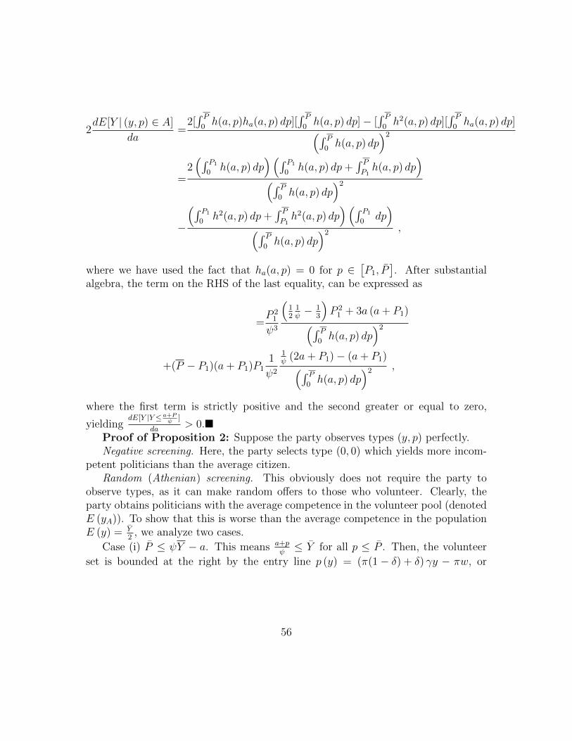
2dE[Y | (y, p) ∈ A]

da=

2[∫ P

0h(a, p)ha(a, p) dp][

∫ P0h(a, p) dp]− [

∫ P0h2(a, p) dp][

∫ P0ha(a, p) dp](∫ P

0h(a, p) dp

)2

=2(∫ P1

0h(a, p) dp

)(∫ P1

0h(a, p) dp+

∫ PP1h(a, p) dp

)(∫ P

0h(a, p) dp

)2

−

(∫ P1

0h2(a, p) dp+

∫ PP1h2(a, p) dp

)(∫ P1

0dp)

(∫ P0h(a, p) dp

)2 ,

where we have used the fact that ha(a, p) = 0 for p ∈[P1, P

]. After substantial

algebra, the term on the RHS of the last equality, can be expressed as

=P 2

1

ψ3

(12

1ψ− 1

3

)P 2

1 + 3a (a+ P1)(∫ P0h(a, p) dp

)2

+(P − P1)(a+ P1)P11

ψ2

1ψ

(2a+ P1)− (a+ P1)(∫ P0h(a, p) dp

)2 ,

where the first term is strictly positive and the second greater or equal to zero,

yieldingdE[Y |Y≤a+P

ψ]

da> 0.�

Proof of Proposition 2: Suppose the party observes types (y, p) perfectly.Negative screening. Here, the party selects type (0, 0) which yields more incom-

petent politicians than the average citizen.Random (Athenian) screening. This obviously does not require the party to

observe types, as it can make random offers to those who volunteer. Clearly, theparty obtains politicians with the average competence in the volunteer pool (denotedE (yA)). To show that this is worse than the average competence in the populationE (y) = Y

2, we analyze two cases.

Case (i) P ≤ ψY − a. This means a+pψ≤ Y for all p ≤ P . Then, the volunteer

set is bounded at the right by the entry line p (y) = (π(1− δ) + δ) γy − πw, or

56

y = p+πw(π(1−δ)+δ)γ = a+p

ψ.

E (yA) =

∫ P0

∫ a+pψ

0 y dydp∫ P0

∫ a+pψ

0 dydp=

∫ P0

12

(a+pψ

)2

dp∫ P0

a+pψdp

=

∫ P0

12a+pψdp∫ P

0dp

=1

2

a+ p

ψ<Y

2= E (y) ,

by the assumption that a+pψ≤ Y .

Case (ii) P > ψY −a. This means a+pψ≤ Y for all p ≤ P1 = ψY −a, but a+p

ψ> Y

for p > P1. Then we have

E (yA) =

∫ P1

0

∫ a+pψ

0 y dydp+∫ PP1

∫ Y0y dydp∫ P1

0

∫ a+pψ

0 dydp+∫ PP1

∫ Y0dydp

=

=

∫ P1

0

∫ a+pψ

0 y dydp∫ P1

0

∫ a+pψ

0 dydp

∫ P1

0

∫ a+pψ

0 dydp∫ P1

0

∫ a+pψ

0 dydp+∫ PP1

∫ Y0dydp

+

∫ PP1

∫ Y0y dydp∫ P

P1

∫ Y0dydp

∫ PP1

∫ Y0dydp∫ P1

0

∫ a+pψ

0 dydp+∫ PP1

∫ Y0dydp

=

∫ P1

0

∫ a+pψ

0 y dydp∫ P1

0

∫ a+pψ

0 dydpα +

∫ PP1

∫ Y0y dydp∫ P

P1

∫ Y0dydp

(1− α) ,

where α ≡∫ P10

∫ a+pψ

0 dydp∫ P10

∫ a+pψ

0 dydp+∫ PP1

∫ Y0 dydp

. Thus,

E (yA) =

∫ P1

012

(a+pψ

)2

dp∫ P1

0a+pψdp

α +

∫ PP1

12Y 2dp∫ P

P1Y dp

(1− α)

=1

2

(a+ p

ψα + Y (1− α)

)<Y

2

since a+pψ

is only defined over values of p such that a+pψ< Y .

Positive screening. This is the only form of screening that can deliver politicianswho, on average, are more able than the average citizen. By continuity, very mildly

57

positive screening – arbitrarily close to random screening – will yield politicians worsethan the population on average. Therefore, positive screening must be pronouncedenough for politicians to be better than the average. Under the assumptions thattypes are perfectly observable and both traits are valuable, the party will select types(P ,min

{P+wπ

(π(1−δ)+δ)γ , Y})

.�

58

who becomes a politician?

Documents