1

Who benefits from universal child care? Estimating marginal

returns to early child care attendance*

Thomas Cornelissen

Christian Dustmann

Anna Raute

Uta Schönberg

This version: August 2016

Abstract

In this paper, we examine the heterogeneous treatment effects of a universal

child care (preschool) program in Germany by exploiting the exogenous

variation in attendance caused by a reform that led to a large staggered

expansion across municipalities. Drawing on novel administrative data from

the full population of compulsory school entry examinations, we find that

children with lower (observed and unobserved) gains are more likely to

select into child care than children with higher gains. This pattern of reverse

selection on gains is driven by unobserved family background

characteristics: children from disadvantaged backgrounds are less likely to

attend child care than children from advantaged backgrounds but have larger

treatment effects because of their worse outcome when not enrolled in child

care.

JEL: J13, J15, I28

Keywords: Universal child care, child development, marginal treatment effects

* Correspondence: Thomas Cornelissen, Department of Economics, University College London

and Centre for Research and Analysis of Migration (CReAM), 30 Gordon Street, London WC1H 0AX,

United Kingdom (email: t.cornelissen@ucl.ac.uk); Christian Dustmann, Department of Economics,

University College London and CReAM, 30 Gordon Street, London WC1H 0AX, United Kingdom

(email: c.dustmann@ucl.ac.uk); Anna Raute, Department of Economics, University of Mannheim, L7,

3-5, 68161 Mannheim, Germany (email: a.raute@uni-mannheim.de); Uta Schönberg, Department of

Economics, University College London, CReAM and IAB, 30 Gordon Street, London WC1H 0AX,

United Kingdom (email: u.schoenberg@ucl.ac.uk).

We are indebted to the Health Ministry of Lower Saxony (NLGA) for providing the data and

particularly grateful to Dr. Johannes Dreesman for his advice and invaluable support with data

management. Christian Dustmann acknowledges funding from the European Research Council (ERC)

under Advanced Grant No. 323992.

2

1. Introduction

Preschool and early childhood programs are generally considered effective means of

influencing child development (see, e.g., Currie and Almond, 2011; Ruhm and Waldfogel,

2012) both because many skills are best learnt when young (e.g., Shonkoff and Phillips, 2000)

and because the longer pay-off period makes such learning more productive (Becker, 1964).

There may also be important “dynamic complementarities” of early learning with acquisition

of human capital at later stages (Cunha and Heckman, 2007; Heckman, 2007; Aizer and

Cunha, 2012). In recognition of these benefits, most European countries, including the U.K.,

France, Germany, and all Nordic nations, offer publicly provided universal child care (or

preschool) programs aimed at promoting children’s social and cognitive development. In the

U.S., which offers no nationwide universal preschool program, an important goal of the Obama

administration’s Zero to Five Plan is to create similar initiatives. Hillary Clinton is proposing a

child care plan which includes universal preschool for 4-year olds as part of her presidential

campaign.1

Yet despite enormous policy interest, evidence of the effectiveness of child care (or

preschool) programs is scarce and far from unified. For example, proponents of child care

programs often cite targeted programs like Head Start or the Perry Preschool Project, which

have generated large long-term gains for participants.2 Evidence on the effectiveness of

universal child care programs targeted at all children, on the other hand, is mixed, with effects

ranging from negative to positive.3 One important reason why targeted child care programs

1 State-level programs (often referred to as pre-K) are currently in place in Georgia, Florida, New Jersey,

New York, and Oklahoma, and have been enacted or expanded in recent years in Alabama, Michigan, Minnesota,

and Montana. A subsidized universal child care program also exists in the Province of Quebec, Canada. 2 See, for instance, the papers by Currie and Thomas (1995), Garces, Currie, and Thomas (2002), Carneiro

and Ginja (2014), Heckman, Moon, Pinto, Savelyev, and Yavitz (2010a,b), and the synthesis in Elango, García,

Heckman and Hojman (2016). 3 For example, whereas Berlinski, Galiani, and Gertler (2009), Berlinski, Galiani, and Manacorda (2008),

Havnes and Mogstad (2011), and Felfe, Nollenberger, and Rodriguez-Planas (2015) find positive mean effects of

an expansion in pre-elementary education in Argentina, Urugay, Norway, and Spain, respectively; Baker, Gruber,

and Milligan (2008, 2015) report negative mean impacts of highly subsidized universal child care in Quebec on

behavioral and health outcomes in the short and longer run. Datta Gupta and Simonsen (2010) also find no

evidence that enrollment in center-based care at age 3 in Denmark improves child outcomes, and Magnuson,

Ruhm, and Waldfogel (2007) find mixed effects of pre-K attendance in the U.S., including positive short-lived

3

yield larger returns than large scale universal programs may be treatment effect heterogeneity;

that is, the former target children from disadvantaged backgrounds who may benefit more from

attending child care programs than the average child, for instance because they experience

lower quality care in the untreated state (i.e., a worse home environment), but a similar

environment in the treated state (because child care programs are of similar quality).4

In this paper, we assess treatment effect heterogeneity in a universal preschool or child care

program aimed at 3- to 6-year-olds in Germany. Our goal is to better understand which

children benefit most from the program and whether treatment effect heterogeneity can help

reconcile the divergent evidence on targeted and universal child care programs. Specifically,

we apply the marginal treatment effects (MTE) framework introduced by Björklund and

Moffitt (1987) and generalized by Heckman and Vytlacil (1999, 2005, 2007), which relates the

heterogeneity in the treatment effect to observed and unobserved heterogeneity in the

propensity for child care enrollment. Such a framework produces a more complete picture of

effect heterogeneity than the conventional IV analysis typically adopted in the literature.

The study context offers two key advantages: First, it allows us to exploit a reform during

the 1990s that entitled every child in Germany to a heavily subsidized half-day child care

placement from the third birthday to school entry. While the reform somewhat increased

attendance rates of 4-year-olds who attend child care for two years, it mainly affected the share

of children who start child care at age 3 and attend childcare for 3 years (an increase from 41%

to 67% on average over the program rollout period). We therefore define our baseline treatment

as attending child care for (at least) 3 years (which we refer to as “early attendance”), but also

show results that explicitly take into account the multivalued nature of our treatment and

distinguish between attending child care for 1, 2 or 3 years. The expansion in publicly provided

effects on academic skills, and negative and more persistent effects on behavioral outcomes. Baker, 2011, and

Elango et al., 2016, provide extensive reviews of this literature. 4 In line with this argument, a recent excellent synthesis of the literature on early childhood education by

Elango et al. (2016) concludes that high-quality programs targeted to children from disadvantaged backgrounds

(including Head Start) have positive effects when the effect is measured against the counterfactual of home care,

but that the effects of universal programs are more ambiguous and crucially depend on the alternative setting that

they are substituting for.

4

child care was staggered across municipalities, creating variation in the availability of child

care slots (our instrument) not only across space but also across cohorts. It thus permits a

tighter design for handling nonrandom selection into child care than is typical in the related

literature that estimates marginal treatment effects. Second, it offers the unique feature that

prior to school entry at age 6, all children must undergo compulsory school entry exams

administered by pediatricians. We have obtained rare administrative data from these school

entry examinations for the entire population of children in one large region, providing us with a

measure of overall school readiness (which determines whether the child is held back from

school entry for another year), as well as measures of motor skills and health, including

information on overweight. These indicators are important predictors of academic success and

health later in life (e.g., Grissmer et al., 2010; Wang et al., 2011).

Unlike many previous studies that use administrative data on child outcomes, we also

observe individual child care attendance, which is crucial to our implementation of the MTE

framework.5 We match the examination data with survey data on the local child care supply in

each municipality and base our instrument on changes in the local availability of child care,

capturing only arguably exogenous changes in supply (conditional on municipality and cohort

effects).

We find substantial heterogeneity in returns to early child care attendance with respect to

both observed and unobserved characteristics. Children of immigrant ancestry (hereafter

referred to as “minority children”) are less likely to attend child care early but experience

higher returns in terms of overall school readiness than native children, which points to a

reverse selection on gains based on observed characteristics. The selection on unobserved

characteristics reinforces this finding: for our primary outcome of overall school readiness,

children with unobserved characteristics that predispose them to early child care entry (“low

5 Most papers exploiting child care reforms focus on intention-to-treat effects, partly because information on

individual child care attendance is unavailable (see, e.g., Baker, Gruber, and Milligan, 2008; Havnes and Mogstad,

2011, 2015; Felfe, Nollenberger, and Rodriguez-Planas, 2015). Without information on individual treatment

status, however, it is impossible to determine whether heterogeneity in intention-to-treat effects is caused by the

differential take-up of children or by heterogeneous responses to child care attendance. For example, larger

intention-to-treat effects at the bottom or middle part of the outcome distribution found by Havnes and Mogstad

(2015) may either be driven by differences in child care take up, or by differences in the impacts of uptake.

5

resistance children”) benefit the least from early child care attendance, whereas those least

likely to enter (“high resistance children”) benefit the most. As a consequence, the effect of

treatment on the untreated (TUT) exceeds the average treatment effect (ATE), which in turn

exceeds the effect of treatment on the treated (TT), with TUT being strongly positive and

statistically significant and TT being negative. We confirm a pattern of reverse selection on

gains when modelling treatment as an ordered choice of attending child care for either 1, 2 or 3

years rather than as a binary decision of attending child care for 3 or less than 3 years. Because

conventional IV methods typically estimate one overall effect, they do not detect such

important treatment effect heterogeneity.

By digging deeper into the reasons for these findings, we show that the higher returns to

treatment for high versus low resistance children are driven by worse outcomes in the untreated

state—which in the German context is almost exclusively family care by either parents or

grandparents—whereas outcomes in the treated state are more homogeneous, in line with the

relatively small quality differences between child care programs in our context. Thus, formal

child care acts as an equalizer. Our results also suggest that high resistance children are more

likely to come from more disadvantaged backgrounds.

What, then, explains the pattern of reverse selection on gains revealed in this paper? One

important reason could be that parental decisions about child care arrangements are based not

only on the child’s welfare but also the parents’ own objectives. For instance, although well-

educated parents could provide their children with a high quality home environment, they may

opt for child care because of their own career concerns and labor market involvement. On the

other hand, mothers from disadvantaged or minority backgrounds not only face higher relative

child care costs but may also have lower incentives to participate in the labor market. They

may also have a more critical attitude toward publicly provided child care, or underestimate the

returns to investment in their children (see Cunha, Elo and Culhane, 2013). At the same time,

the home environment may deprive the children of exposure to peers and the learning activities

6

provided in child care, thereby delaying development.6 Moreover, throughout the expansion

period, child care decisions were not only made by parents, but in case of excess demand also

by child care centers. The allocation mechanism adopted by centers, which in addition to the

child’s age as the primary admission criterion was based on mothers’ employment status and

time on the waiting list, may have favored majority and advantaged children—since majority

and high-skilled mothers are more likely to participate in the labor market and also likely to be

better informed about the specific admission process than minority and low-skilled mothers.

In addition to highlighting the importance of heterogeneity in both the “resistance” to child

care enrollment and in children’s responses to child care attendance, our findings also reconcile

the seemingly contradictory results of positive effects for programs targeted at disadvantaged

children but mixed effects for universal programs. In terms of relevant policy implications,

they suggest that parental choices may differ from those that the children themselves would

make, potentially supporting the claim that state involvement in the early child care market

may “[…] mimic the agreements that would occur if children were capable of arranging for

their [own] care” (Becker and Murphy, 1988, p. 1). Our results also imply that policies which

successfully attract high resistance children not currently enrolled in early child care may yield

large returns. Further, programs targeted at minority and disadvantaged children are likely to

be more cost effective and beneficial than universal child care programs.

Our paper makes several important contributions. The sparse research on heterogeneity in

returns to child care typically focuses on treatment heterogeneity in observed characteristics, or

estimates quantile treatment effects (QTE) rather than marginal treatment effects, as we do. For

example, consistent with our findings, Cascio and Schanzenbach (2013) show that the

universal preschool programs in Georgia and Oklahoma improved test score outcomes of

children from low-income families as late as 8th

grade, but had little impact on children from

6 The positive correlation between parental inputs and parental socioeconomic background is well

documented. For example, Guryan, Hurst, and Kearney (2008) provide evidence for a positive relation between

maternal education and time spent with children for both nonworking and working mothers. Hart and Risley

(1995) and Rowe (2008) also report that low SES mothers talk less and use less varied vocabulary during

interaction with their children than high SES mothers, with the latter hearing approximately 11,000 utterances a

day compared to 700 utterances for (Hart and Risley, cited in Rowe, 2008).

7

high-income families. In a similar vein, Havnes and Mogstad (2015), by estimating quantile

treatment effects and local linear regressions by family income, show that children of low

income parents benefit substantially from the child care expansion studied, whereas earnings of

upper class children may have suffered.7 Bitler, Hoynes, and Domina (2016) identify the

strongest distributional effects for the Head Start program among children in the lower part of

the outcome distribution. The MTE approach adopted in our study allows us to not only

uncover treatment heterogeneity in observed characteristics (as in Cascio and Schanzenbach,

2013), but also in unobserved characteristics. In addition, it has a number of advantages over

the QTE approach adopted by Havnes and Mogstad (2015) and Bitler, Hoynes, and Domina

(2016): unlike the QTE approach, it does not hinge on a rank invariance assumption,8 and by

relating treatment effects to the participation decision, the nature of selection into treatment can

be determined and various treatment effects like TT and TUT can be computed.

The only two recent studies we know of that use an MTE framework to estimate

heterogeneity in returns to early child care attendance with respect to unobserved

characteristics are Kline and Walters (2016) and Felfe and Lalive (2015). The former evaluates

a targeted child care program (Head Start) with an emphasis on multiple untreated states (i.e.,

home care vs. other subsidized public child care), whereas the latter examines a younger

population of mostly 1 and 2-year old children. We, in contrast, study a universal child care

program in which the untreated state is almost exclusively home care, and concentrate on 3- to

4-year old children who are at the heart of the current policy debate in the U.S. and Europe.9

Our study also contributes to the growing literature that estimates marginal treatment

effects in different contexts, most of which has focused on returns to schooling at the college

7 Using a similar approach, Kottelenberg and Lehrer (2016) find substantial heterogeneity in distributional

effects for the Quebec Family Policy. 8 The rank invariance assumption (or rank preservation, see Elango et al., 2015) is necessary to interpret the

QTE as the treatment effect of the individual at the qth

quantile of the outcome distribution in the untreated state

and implies, as discussed by Chernozhukov and Hansen (2005), that a common unobserved factor determines the

ranking of a given person in both the treated and untreated state. The MTE approach, in contrast, allows

unobserved factors to differently affect outcomes in the treated and untreated states. 9 In line with our findings and consistent with Bitler, Hoynes, and Domina (2016), Kline and Walters (2016)

uncover a pattern of reverse selection on gains for Head Start attendance when the nontreated state is home care.

Felfe and Lalive (2015), in contrast, do not find general evidence for reverse selection on gains, possibly because

they study the effects of child care attendance for a younger group of children than we do.

8

(see, e.g., Carneiro, Heckman, and Vytlacil, 2011, for the U.S.; Balfe, 2015, for the U.K.;

Nybom, 2014, for Sweden) or secondary school level (e.g., Carneiro, Lokshin, Ridao-Cano,

and Umapathi, 2015), typically producing evidence for a strong self-selection into treatment

based on net gains.10

Our findings, in contrast, show that when someone other than the

treatment subject (e.g., the parents or an administrator) decides on enrollment (the

intervention), the relation between selection and gains may be reversed so that individuals with

the highest enrollment resistance benefit most from the treatment.11

We deviate from the existing MTE literature in the field of education by adopting a tighter

identification strategy that exploits variation in the instrument not only across areas (the main

variation used in existing studies) but also across cohorts, thus enabling us to control for time-

constant unobserved area characteristics. An additional strength is that the exogenous variation

from a strong, sustained expansion of child care slots creates common support in the estimated

(unconditional) propensity score over virtually the full unit interval. While rare in MTE

applications, this is crucial to compute the TT and the TUT, which heavily weight individuals

at the extremes of the treatment propensity distribution, without having to extrapolate out of

the common support.12

The paper proceeds as follows. Section 2 outlines the empirical framework and the method

for estimating the marginal returns to child care attendance. Sections 3 and 4 describe the data,

the main features of the German public child care system, and the child care reform. Section 5

reports our main findings on treatment effect heterogeneity and its relation to the pattern of

selection into treatment. Section 6 then offers a possible explanation for the main pattern of

10

An important exception (in a context other than early child care attendance) is Aaakvik, Heckman, and

Vytlacil (2005) who find evidence in line with the reverse selection on gains in context of a vocational

rehabilitation program in Norway. As in our context, the decision whether to enroll in the program is a joint

decision by the case-worker and the individual. The unexpected pattern of reverse selection may be explained by

cream-skimming of individuals into training by case-workers on the basis of their employability rather than their

marginal gains from training. 11

The MTE framework has also been applied to measure the marginal treatment effects of foster care on

future outcomes (Doyle, 2007), heterogeneity in the impacts of comprehensive schools on long-term health

behavior (Basu, Jones, and Rosa Dias, 2014), and heterogeneity in the effects of disability insurance receipt on

labor supply (Maestas, Mullen, and Strand, 2013; French and Song, 2014). 12

For instance, the common support in French and Song (2014) ranges from 0.45 to 0.85 (as depicted by

French and Taber (2011), while that in Felfe and Lalive (2015) ranges only between 0 and 0.5. Carneiro,

Heckman, and Vytlacil (2011), in contrast, achieve nearly full common support by combining four different

instruments.

9

findings and discusses policy simulations. Section 7 concludes the paper with a discussion of

policy implications.

2. Estimating marginal returns to child care attendance

2.1 Baseline model set up (Binary treatment)

We assess the extent and pattern of treatment effect heterogeneity with respect to both

observed and unobserved characteristics using the MTE framework proposed by Björklund and

Moffitt (1987) and subsequently developed in a series of papers by Heckman (1997) and

Heckman and Vytlacil (1999, 2005, 2007). We use 𝑌0𝑖 and 𝑌1𝑖 to denote the potential outcome

(from the school entrance exams) for individual i in the nontreated versus the treated state,

respectively (with 𝐷𝑖 = 1 denoting treatment). We model the potential outcomes 𝑌𝑗𝑖 as a

function of the observed control variables 𝑋𝑖 (e.g., child gender, age, and minority status) and

dummies for municipality (𝑅𝑖) and examination cohort (𝑇𝑖):

𝑌𝑗𝑖 = 𝑋𝑖𝛽𝑗 + 𝑅𝑖𝛼 + 𝑇𝑖𝜏 + 𝑈𝑗𝑖, 𝑗 = 0,1. (1)

Following Brinch, Mogstad, and Wiswall (2016), we interpret equation (1) as a linear

projection of 𝑌𝑗 on (𝑋, 𝑅, 𝑇), which implies that by definition, 𝑈𝑗 is normalized to [𝑈𝑗|𝑋 =

𝑥, 𝑅 = 𝑟, 𝑇 = 𝑡] = 0. 13

For selection into treatment 𝐷𝑖 (defined in our baseline specification as child care

attendance for at least 3 years), we use the following latent index model:

𝐷𝑖∗ = 𝑍𝑖𝛽𝑑 − 𝑉𝑖

𝐷𝑖 = 1 if 𝐷𝑖∗ ≥ 0, 𝐷𝑖 = 0 otherwise, (2)

where 𝑍 = (𝑋, 𝑅, 𝑇, �̃�), implying that 𝑍 includes the same covariates (𝑋, 𝑅, 𝑇) as the outcome

equation (1) and an instrument �̃� excluded from the outcome equation.14

In our application, �̃�

13

The coefficient vector, defined as (𝛽𝑗 𝛼 𝜏)′ = [(𝑋, 𝑅, 𝑇) ′(𝑋, 𝑅, 𝑇) ]−1(𝑋, 𝑅, 𝑇) ′𝑌𝑗, should therefore be

interpreted in terms of partial correlations rather than as a causal or structural parameter. Other studies, such as

Aakvik, Heckman, and Vytlacil (2005), Carneiro et al. (2011) and Carneiro et al. (2015) instead invoke

independence of (𝑋, 𝑅, 𝑇) and 𝑈𝑗, in which case (𝛽𝑗 𝛼 𝜏)′ and 𝑈j are defined as structural or causal.

14 As Vytlacil (2002) points out, additive separability between 𝑍𝑖𝛽𝑑 and 𝑉𝑖 in the latent index model in

equation (2) implies monotonicity (or more appropriately uniformity): a change of the propensity score from P(Z)

to P(Z’) either shifts all individuals into treatment or out of treatment.

10

is local child care supply as measured by the child care coverage rate 3 years prior to the school

entrance examination. Because the error term 𝑉𝑖 enters the selection equation (2) with a

negative sign, it embodies the unobserved characteristics that make individuals less likely to

receive treatment. We thus label 𝑉𝑖 “unobserved resistance” or “distaste” for treatment.

Equation (1) implies that the individual treatment effect (the difference between the

potential outcomes in the treated and untreated states) is given by 𝑌1𝑖 − 𝑌0𝑖 = 𝑋𝑖(𝛽1 − 𝛽0) +

𝑈1𝑖 − 𝑈0𝑖. Treatment effect heterogeneity may thus result from both observed (differences

between 𝑋𝑖𝛽1 and 𝑋𝑖𝛽0) and unobserved characteristics (differences between 𝑈1𝑖 and 𝑈0𝑖).15

A

key feature of the MTE approach is that it allows the unobserved gain from treatment (𝑈1𝑖 −

𝑈0𝑖) to be correlated with unobserved characteristics that affect selection (𝑉𝑖). In the remainder

of the exposition, we drop the i index to simplify notation.

In the MTE literature, it is customary to trace out the treatment effect against the quantiles

of the distribution of 𝑉 rather than against its absolute values, in line with the following

transformation of the selection rule in equation (2): 𝑍𝛽𝑑 − 𝑉 ≥ 0 ⇔ 𝑍𝛽𝑑 ≥ 𝑉 ⇔ Φ(𝑍𝛽𝑑) ≥

Φ(𝑉), with Φ denoting the c.d.f. of 𝑉 (in our application, a standard normal distribution). The

term Φ(𝑍𝛽𝑑), also denoted by Φ(𝑍𝛽𝑑) ≡ 𝑃(𝑍), is the propensity score (the probability that an

individual with observed characteristics 𝑍 will receive treatment), and Φ(𝑉), denoted

by Φ(𝑉) ≡ UD, represents the quantiles of the distribution of unobserved resistance to

treatment 𝑉. The marginal treatment effect as a function of these quantiles can then be

expressed as

MTE(𝑋 = 𝑥, UD = 𝑢𝐷) = 𝐸(𝑌1 − 𝑌0|𝑋 = 𝑥, UD = 𝑢𝐷),

where MTE is the gain from treatment for an individual with observed characteristics 𝑋 = 𝑥

who is in the 𝑢𝐷-th quantile of the 𝑉 distribution, implying the individual is indifferent to

receiving treatment when having a propensity score 𝑃(𝑍) equal to 𝑢𝐷.

15

Because the municipality and year dummies are restricted to having the same effect in the treated and

untreated outcome equations, they have no influence on the treatment effect. We allow all other covariates in X to

have different effects in treated versus untreated cases except for a set of birth month dummies.

11

We impose the following assumptions. First, there must be a first stage in which the

instrument �̃� (the child care coverage rate in the municipality) causes variation in the

probability of treatment after controlling for (𝑋, 𝑅, 𝑇). This relation does indeed exist in our

application (see Section 5.1 and Table 4). Second, �̃� must be independent of the unobserved

component of the outcome and selection equation conditional on the observed characteristics

and the municipality and cohort dummies; that is, �̃� ⫫ (𝑈0, 𝑈1, 𝑉) | (𝑋, 𝑅, 𝑇). This assumption

requires that the instrument be as good as randomly assigned conditional on (𝑋, 𝑅, 𝑇). It also

embodies the exclusion restriction that the child care coverage rate in the municipality 3 years

prior to the school entry examination must not directly affect the examination outcome

conditional on 𝐷𝑖 and (𝑋, 𝑅, 𝑇). It further implies that the way in which 𝑈1 and 𝑈0 depend on 𝑉

(i.e., the MTE curve) must not depend on �̃�; we present evidence supporting the validity of our

instrument in Section 4.3. Third, following Brinch, Mogstad, and Wiswall (2016), we assume

that the marginal treatment effect is additively separable into an observed and an unobserved

component:

MTE(𝑥, 𝑢𝐷) = 𝐸(𝑌1 − 𝑌0|𝑋 = 𝑥, UD = 𝑢𝐷)

= 𝑥(𝛽1 − 𝛽0)⏟ obsered component

+ 𝐸(𝑈1 − 𝑈0|UD = 𝑢𝐷)⏟ unobserved component

, (3)

Accordingly, the treatment effect heterogeneity resulting from the observed characteristics 𝑋

affects the intercept of the MTE curve as a function of 𝑢𝐷 but its slope in 𝑢𝐷 does not depend

on 𝑋. This separability is a common feature of empirical MTE applications because it

considerably eases the data requirements for estimating the MTE curve.16

Most importantly, it

allows identifying the MTE over the unconditional support of 𝑃(𝑍), jointly generated by the

excluded instrument and the covariates, as opposed to the support of 𝑃(𝑍) conditional on X=x

(Carneiro, Heckman and Vytlacil, 2011).

16

The existing literature typically invokes the stronger assumption of full independence between (X, R, T, 𝑍)

and (U0, U1UD); for example, Aakvik, Heckman, and Vytlacil, 2005; Carneiro, Heckman, and Vytlacil, 2011;

Carneiro, Lokshin, Ridao-Cano, and Umapathi, 2014).

12

2.2 Estimation

We estimate the MTE using the local instrumental variable estimator, exploiting the fact that

the model described in Section 2.1 produces the following outcome equation as a function of

the observed regressors X and the propensity score 𝑃(𝑍) = 𝐸[𝐷 = 1|𝑍] (cf. Heckman, Urzua,

and Vytlacil, 2006; Carneiro, Heckman, and Vytlacil, 2011):

𝐸[𝑌|𝑋 = 𝑥, 𝑅 = 𝑟, 𝑇 = 𝑡, 𝑃(𝑍) = 𝑝] = 𝑋𝛽0 + 𝑅𝛼 + 𝑇𝜏 + 𝑋(𝛽1 − 𝛽0)𝑝 + 𝐾(𝑝),

where 𝐾(𝑝) is a nonlinear function of the propensity score. As shown by Heckman, Urzua, and

Vytlacil (2006) and Carneiro, Heckman, and Vytlacil (2011), the derivative of this outcome

equation with respect to 𝑝 delivers the MTE for 𝑋 = 𝑥 and 𝑈𝐷 = 𝑝:17

𝜕𝐸[𝑌|𝑋 = 𝑥, 𝑃(𝑍) = 𝑝]

𝜕𝑝= 𝑋(𝛽1 − 𝛽0) +

𝜕𝐾(𝑝)

𝜕𝑝= MTE(𝑋 = 𝑥, 𝑈𝐷 = 𝑝).

We implement this approach by first estimating the treatment selection equation in (2) as a

probit model to obtain estimates of the propensity score �̂� = Φ(𝑍�̂�𝑑) and then modeling 𝐾(𝑝)

as a polynomial in 𝑝 of degree k and estimating the outcome equation:

𝑌 = 𝑋𝛽0 + 𝑅𝛼 + 𝑇𝜏 + 𝑋(𝛽1 − 𝛽0)�̂� +∑𝛼𝑘�̂�𝑘

𝐾

𝑘=2

+ 𝜀. (4)

The MTE curve is then the derivative of equation (4) with respect to �̂�. We assume a second

order polynomial in �̂� (K=2) in our baseline specification, but generally find similar results for

K=3, K=4 and a semiparametric specification of 𝐾(𝑝). To assess whether treatment effects

vary with the unobserved resistance to treatment, we run tests for the joint significance of the

second and higher order terms of the polynomial (i.e., the 𝛼𝑘 in equation (4)).18

17

The derivative of the outcome with respect to the observed inducement into treatment (the propensity

score) yields the treatment effect for individuals at a given point in the distribution of the unobserved resistance to

treatment (𝑈𝐷) because of the following. First, given a propensity score with the specific value of 𝑝 = 𝑝0,

individuals with 𝑈𝐷 < 𝑝0 are treated while individuals with 𝑈𝐷 = 𝑝0 are indifferent. If 𝑝 is increased from 𝑝0 by a

small amount 𝑑𝑝, previously indifferent individuals with 𝑈𝐷 = 𝑝0 are shifted into treatment with a marginal

treatment effect of MTE(𝑈𝐷 = 𝑝0). Outcome Y then increases by the share of shifted individuals times their

treatment effect, dY=dp* MTE(𝑈𝐷 = 𝑝0), and the derivative of Y with respect to dp normalizes dY by dp (the

change in the explanatory variable), dY/dp= MTE(𝑈𝐷 = 𝑝0). The derivative of the outcome with respect to the

propensity score thus yields the MTE at 𝑈𝐷 = 𝑝. 18

We estimate the model using our own modified and extended version of the Stata margte command (see

Brave and Walstrum, 2014).

13

The MTE can be aggregated over UD in different ways to generate several meaningful

mean treatment parameters, such as the effect of treatment on the treated (see Heckman and

Vytlacil, 2005, 2007). In this paper, we compute the unconditional treatment effects by

aggregating the MTE in equation (3) not only over UD but also over the appropriate

distributions of the covariates (see Cornelissen et al., 2016 for a description of the weights).

We report bootstrapped standard errors throughout with clustering at the municipality level.

3. Data

Our main data source is a set of 1994–2006 administrative records for one large region in

West Germany, the Weser-Ems region in Lower-Saxony.19

These records, which represent an

unusually wide array of results for the school readiness examination administered by licensed

pediatricians, cover the full population of school entry aged children. We combine these data

with data on the local supply of child care slots obtained from our own survey, as well as with

data on sociodemographic municipality characteristics and local child care quality measures,

both computed from social security records. This combination of different data sources

produced an extremely rich, high quality data set that is unavailable for other countries.

3.1 School entrance examination

A unique feature of the German school system is that in the year before entering

elementary school, all children undergo a compulsory school entry examination designed to

assess their school readiness and identify any developmental delays or health problems needing

preventive treatment in the future. Typically administered in a nearby elementary school in the

child’s municipality between the February and June before August school entry, the 45-minute

test, conducted by government pediatricians, includes an interview with the child, as well as a

battery of tests of motor skills and physical development. Hence, a major important advantage

19

The region is mostly rural and the two largest cities are home to 270,000 and 160,000 inhabitants,

respectively.

14

of our outcomes is that they represent standardized assessments by health professionals rather

than subjective assessments by parents, which may be prone to a number of sources of bias.20

Our main variable is an indicator variable equal to 1 if the pediatrician assesses the child as

ready for school entry in the fall. Because the pediatricians base such recommendations on all

school entry tests and general observations of the child during the examination, this outcome

serves as a summary measure of all readiness assessments. According to official guidelines,

delayed school entry is recommended in the case of major physical, cognitive, or emotional

developmental delays and if any therapeutic or special needs measures will not generate school

readiness before the start of school. Similar indicators used to assess school preparedness in the

U.S. have proven to be important predictors for later academic success (e.g., Duncan et al.,

2007; Grissmer et al., 2010; Pagani et al., 2010). Since parents and schools almost always

comply with the pediatrician’s recommendation, deferment from school entry also leads to

significant earnings losses later in life through delayed entry into the labor market.21

For

example, Dustmann, Puhani, and Schönberg (2016) show that in Germany, delayed school

entry leads to 2.3% lower earnings between 30 and 45.22

Likewise, our own calculations based

on the earnings profiles of all men born between 1961 and 1964, discounted to age 3 using a

discount factor of 0.97, suggest that delayed school entry lowers lifetime earnings by €16,878

($22,397) in 2010 prices.23

In addition to our central measure of school readiness, we investigate further more specific

examination outcomes: a diagnosis of motor skill problems (based on balancing, jumping, and

20

Heckman and Kautz (2014) and Baker, Gruber, and Milligan (2008) provide a detailed discussion on this

issue, and Sandner and Jungmann (2016) show that bias in maternal ratings of early child development is related

to socio-economic status. 21

In 2005, the actual deferment rate in our region was nearly identical to the deferment rate recommended by

the pediatrician (author calculations based on data from the Lower Saxony State Office of Statistics, 2005). 22

Dustmann, Puhani, and Schönberg (2016) report that individuals born in June are 21.9 percentage points

more likely to start school at age 6 than those born in July (see Appendix A.2). At the same time, the wages of 30-

to 45-year-old men born in July are 0.5% lower than men of the same age group born in July (compare column

(1), panel A, and row (i) of Table 3 in Dustmann, Puhani, and Schönberg, 2016), suggesting that delaying school

entry by one year reduces wages by 2.3%. 23

Available evidence from the US and Norway is broadly consistent with the findings for Germany. For

example, Deming and Dynarski (2008) conclude that “there is substantial evidence that entering school later …

depresses lifetime earnings (by delaying entry into the job market” (page 72). Black, Devereux and Salvanes

(2011) examine the effect of school starting age for Norway and show that delaying school entry leads to lower

earnings until about age 30.

15

ball exercise tests for body coordination);24

the logarithm of the child’s body mass index (BMI)

and a binary indicator for overweight, as two important predictors of adult health (Ebbeling,

Pawlak, and Ludwig, 2002; Wang et al., 2011); and a physician recommendation for

compensatory sport when the child shows any postural or coordination problems, lack of

muscular tension, or psychosomatic developmental problems. For child overweight, we follow

the official German pediatric guidelines of a BMI above the 90th

percentile of the age- and

gender-specific BMI distribution (see Kromeyer-Hauschild et al., 2001). Our data also include

the number of years a child has spent in public child care (information rarely available in

administrative data sources) but only contain parental background information (e.g. education)

from 2001 onward. Therefore we only exploit the latter in an auxiliary analysis.

From this data set, we sample all children examined for the first time between 1994 and

2002, which are the school entry cohorts most affected by the child care program expansion

(see Section 4.2). We further restrict the sample to municipalities for which we have data on

available child care slots (see Section 3.2 below), which yields a baseline sample of 135,906

children in 80 municipalities. As Table 1, panel A shows, 51% of the children in this final

sample attended child care for at least 3 years (our baseline treatment variable).25

Children of

immigrant ancestry make up about 12% of our sample. Although 91% of all the children

examined were assessed as ready for immediate school entry, considerable individual

heterogeneity is observable in this measure: based on a probit regression using the same

covariates as in our baseline specification, predicted school readiness ranges from 0.31 to 1 and

is less than 0.79 for 10% of children. It should be noted that these numbers capture individual

heterogeneity in school readiness based on observed characteristics only: individual

heterogeneity based on unobserved characteristics is likely to be even larger. Regarding the

other outcomes, 85% of the children showed no lack of motor skills, 82% had no need for

compensatory sport, and only 8% of the children could be classified as overweight.

24

In our data, motor skill problems take four values depending on the severity of the abnormality. As very

severe levels are a rare outcome and the multivalued outcome variable lacks a meaningful cardinal scale (see

Cunha and Heckman, 2008), we have transformed them into binary outcome variables. 25

Only 5.6% of the children in our sample attended child care for longer than 3 years, so the vast majority

(88%) of treated children attended child care for 3 years.

16

We provide additional information on minority children in Panel B of Table 1. 35% of

minority children are ethnic Germans from the former Soviet Union whose parents arrived in

Germany mostly in the early 1990s after the breakdown of the Eastern European communist

regimes. Children of Turkish descent form the second largest immigrant group, making up

roughly 30% of immigrant children in our sample. While both minority groups come from less

educated family backgrounds than German children, children of Turkish origin are more

disadvantaged and are less likely to speak German at home with at least one family member

than children from the former Soviet Union, even though the Turkish arrived in Germany

predominantly in the 1960s and 1970s.26

3.2 Data on child care slots

We supplement the school entrance examination data with information on the number of

child care slots available in each year and municipality, collected individually from regional

youth welfare offices for lack of a central source. For the handful of municipalities that could

not provide us with such information, we successfully contacted all child care centers in the

municipality via email and telephone interviews. Overall, we were able to gather detailed

information on child care provision during 1990–2003 for 81 of the 118 municipalities in our

data set, encompassing around 77% of all the children examined.

3.3 Sociodemographic municipality characteristics and local child care quality

We also supplement the examination information with yearly data on local

sociodemographic and child care quality characteristics measured at the municipality level.

Municipality characteristics include the number of inhabitants, median wage, and the share of

individuals with medium and tertiary education in the workforce, as well as the share of

immigrants and women in the workforce obtained either from the statistical office of Lower

Saxony or computed from social security records on all men and women covered by the social

security system in the region. Local child care quality indicators are derived from social

security records on all child care teachers employed in the region with a focus on two

26

See Casey and Dustmann, 2008, for additional evidence on language usage of minority groups in Germany.

17

characteristics identified as central to child care program success (cf. Walters, 2015): class size

and teacher education (see, e.g., Chetty et al., 2011). We also consider the presence of male

child care teachers, which is allowed to affect outcomes differently by gender. The summary

characteristics of the child care quality measures, reported in Table 1, panel C, reveal a median

child-to-staff ratio of 9.4, an average share of 9% of child care teachers with a university

degree, and a male staff share of 2%.27

4. Background

4.1 Child care provision in Germany

To facilitate interpretation of our findings, we first briefly outline the main elements of

formal child care provision for 3- to 6-year-olds in Germany, which is almost exclusively

public. As in other countries, the German universal child care program is a half-day program

with strict nationwide quality standards: the student-teacher ratio must not exceed 25 children

per 2 teachers and teachers must have completed at least a two-year state-certified vocational

program followed by a one-year internship as a child care teacher. Other regulations govern the

space provided for each child, and learning goals pursued by the centers. Overall, these

standards lead to a relatively homogenous child care environment compared to, for example,

the U.S.

In terms of quality standards, Germany occupies an intermediate position in the

international context: the 12.5:1 student-teacher ratio lies between the 8:1 ratio for 3- to 7-year-

olds in U.K. center-based programs, the maximum ratio of 10:1 in the U.S. Head Start

program, and the 25:1 ratio in French programs (OECD, 2006). As of 2002, the estimated

annual expenditure per child in Germany was $4,998, comparable to that of other continental

European universal child care programs (e.g., $4,512 in France; $4,923 in the Netherlands) but

well below high quality intensive programs like Head Start, which invests about $7,200 per

child (OECD 2005, 2006).

27

Child care teachers in Germany mostly have a vocational degree, which is equivalent to a community

college degree in the U.S. University degrees among child care workers are less common, so the 9% of staff with

a university degree are likely to be center managers.

18

As in most universal child care programs, the majority of children in Germany (over

90%)28

attend child care part time for 4 hours in the morning. Most children start child care in

August with the start of the new “preschool year”, and once enrolled, nearly all children remain

in child care until school entry at the age of 6. As is typical for the age group considered,

learning is mostly informal and play oriented, and carried out in the context of day-to-day

social interactions between children and teachers. Like the U.S. HighScope (Ypsilanti)

program or U.K. Early Years Foundation Stage (see Samuelsson, Sheridan, and Williams,

2006, and the Department for Education, 2014 for descriptions), the programs emphasize as

their main learning goals personal and emotional development, social skills, the development

of cognitive abilities and positive attitudes toward learning, physical development, creative

development, and language and communication skills. An important additional element of

German formal child care (and similar programs) is communication with parents to inform

them about their children’s developmental and learning progress and provide them with

educational guidance.

4.2 The child care expansion policy

In Germany, child care for children aged 3 to 6 is heavily subsidized, with parental fees

covering on average only about 10% of the overall child care costs and the remainder shared by

the municipality and state government. Until the early 1990s, however, legal definitions of how

the state and local municipalities should share child care provision responsibilities were vague

and subsidies for the creation of formal child care slots were limited. As a result, such slots

were severely rationed and existing slots were always filled. Waiting lists existed at all child

care centers and were long. At this time, open slots were primarily allocated according to the

child’s age—so 3-year-olds were the most affected by the rationing—and the mother’s labor

force status, with children of working mothers given priority over children of non-working

mothers. In case two children were of the same age, and their mothers were both working, the

application date and time on the waiting lists were the decisive factors. Then, in August 1992,

28

This calculation is based on data from the Statistical Report on Child Care Institutions from the Lower

Saxony State Office for Statistics (Niedersächsisches Landesamt für Statistik, 2004, p. 19).

19

after the burden imposed on families by low child care availability had dominated the political

discussion for well over a year, the federal government introduced a legal mandate that by

January 1, 1996, every child would be guaranteed a subsidized 4-hour slot from the third

birthday until school entry. Although slot provision would be the responsibility of the

residential municipality, the state would provide generous financial aid for the construction and

running of child care facilities. Municipalities with relatively lower child care coverage rates

would be eligible for the highest subsidies. Despite these subsidies, however, creating child

care slots imposed too many constraints on municipalities, so the introduction of the legal

mandate by January 1, 1996, was no longer considered feasible. Consequently, the state

government of Lower Saxony allowed exceptions until December 31, 1998.

Overall, between 1992 and 2002, around 11,000 new child care slots were created for

children aged 3 to 6 in the 80 municipalities in our sample (an increase of close to 40%). Part A

of Figure 1 plots the evolution of the child care coverage rate, computed as the number of

available child care slots in a municipality 3 years prior to the school entry examination (i.e.,

when the child was approximately aged 3), divided by the number of 3- to 6-year-old children

living in that municipality at that time. Coverage increases strongly from 0.59 slots per eligible

child in the 1994 examination cohort to just over 0.8 slots for those in the 2002 examination

cohort. Part B of Figure 1 plots the proportion of children who attended child care for 1, 2 or

(at least) 3 years for the 1994–2002 examination cohorts. The figure reveals that the expansion

in child care slots mostly increased the 3-year attendance rate (i.e., enrolment at age 3) and

reduced the 2-year attendance rate (i.e., enrolment at age 4)—as we would expect since prior to

the expansion preference was given to older children when demand was excessive. Among

children in the 1994 examination cohort (who would have entered child care at the earliest in

1991 before child care expansion), around 41% attended for the full 3 years. For children

examined in 2002, who benefited fully from the child care extension, the 3-year attendance rate

rose to 67%, an increase of nearly 63% compared to 1994. This observation motivates our

20

decision to define treatment in our baseline specification as attending child care for 3 years (or

“attending child care early”).

Although the expansion in child care slots primarily shifted children from attending child

care for 2 years to attending child care for 3 years, panel B also reveals a drop in the 1-year

attendance rate, from 15% for the 1994 examination cohort to 6% for the 2002 examination

cohort. Therefore, the expansion also induced some children to attend child care for 2 (or more)

years rather than 1 year only.29

In Section 5.6, we explicitly take into account the multivalued

nature of our treatment and distinguish between attending child care for 1, 2 or 3 years.

4.3 Exogeneity of the child care expansion

Because the child care expansion was staggered across time and municipalities, in the

empirical analysis we are able to exploit sharp shifts in the supply within municipalities across

nearby cohorts. Specifically, we use the child care coverage rate in t-3 (3 years before the

school entry exam at approximately age 3 when parents decide to enroll their child in early

child care) as an instrument for early child care attendance conditional on municipality and

cohort dummies, thereby accounting for time-constant differences across municipalities (such

as residential sorting). This identification strategy is tighter than typically adopted in the MTE

literature on returns to schooling, which mainly employs spatial variation in instruments.

For the instrument to be valid, the timing and intensity of the child care expansion must be

as good as random (cf. the second assumption discussed in Section 2.1). In column (1), Table

2, we obtain an initial picture of which municipalities in our sample experienced an above-

average 1994–2002 expansion in child care slots by regressing the change in child care

coverage between 1991 and 1999 (i.e., from our 1994 [oldest] cohort’s child care attendance in

t-3 to our 2002 [youngest] cohort’s attendance) on the initial coverage rate in 1991. As

expected, the change in child care supply is strongly negatively related to its baseline

availability, reflecting both the higher state subsidies received by municipalities with lower

29

The non-attendance rate, in contrast, remained roughly constant, suggesting that the expansion did not shift

children into child care who previously had not attended at all.

21

initial coverage rates and the greater political pressure they felt to expand availability relative

to municipalities with higher initial coverage rates. Then, in column (2), we add a number of

baseline (1990) municipality characteristics, including the median wage and the shares of

medium and highly skilled individuals in the workforce. Reassuringly, only one of these

baseline characteristics helps to predict the size of the child care expansion in the municipality

(either individually or jointly); rather, the initial coverage rate remains strongly correlated with

the expansion intensity. However, even if the municipality characteristics at baseline did

predict child care expansion in the municipality, it would not generally invalidate our

identification strategy because these characteristics at baseline mostly reflect time-constant

differences, which are accounted for by the inclusion of municipality dummies in our

estimation.

In addition to exploiting across-municipality variation in expansion intensity, we also

investigate whether the timing of the creation of child care slots is quasi-random. To do so, we

regress the child care coverage rates per 3- to 6-year-old in t-3, our instrument, on socio-

demographic municipality characteristics measured in t-4 (i.e., one year prior to the

measurement of child care availability, to account for the fact that the effect of socio-economic

characteristics on the expansion is unlikely to be instantaneous) while conditioning on

municipality and cohort dummies. As Table 3 shows, none of the municipality characteristics

is statistically significant, and changes in the municipality’s socioeconomic characteristics

appear to be uncorrelated with changes in the child care supply. Hence, the results in both

Table 2 and Table 3 support our identifying assumption that both the intensity and timing of

new child care slot creation are plausibly exogenous. Nevertheless, as a robustness check, we

also report results from a specification that exploits solely variation across municipalities in the

intensity, but not the timing, of child care slot creation (see Section 5.5).

Another threat to identification is the possibility that child care expansion could crowd out

other public expenditure or reduce household income, which might negatively affect child

outcomes. Two factors limit this concern: because income taxes are set on the federal level,

22

municipalities could not increase them to finance the increased child care expenditure, and

because social and unemployment benefits are regulated at the federal level, they are

independent of local government finances. An additional threat is that child care expansion

might negatively change child care quality, affecting not only children pulled into child care by

the creation of new slots but also those whose child care attendance is unaffected. To assess

this possibility, in our baseline specification, we condition on the child care quality measures

available in our data, including child-teacher ratio, teacher education, and teacher gender. We

find that excluding the child care quality measures has little effect on our results (see Section

5.5). A final threat is endogenous mobility: families with strong preferences for early child care

attendance may move to municipalities with a larger supply of child care. In our sample,

however, this bias is unlikely to be a concern, not only because only 4.4% of the families

moved to a new municipality in the 2 years prior to the examination but also because the

mobility rate is uncorrelated with changes in municipal child care availability.30

5. Results

5.1 First-stage selection equation

We display the parameter estimates for the first-stage probit selection equation (2) in the

first column of Table 4.31

To allow for the possibility that at high levels of coverage, when

excess demand eases, the likelihood of filling an additional slot may decrease, we use as

instruments not only the child care coverage rate (centered around its mean) in the municipality

3 years prior to the examination, but also its square. We further interact our instruments with

individual child care characteristics (minority status, gender, and age) to allow for the

30

Regressing the share of families that moved to a new municipality during the previous 2 years on the

number of available child care slots as measured by the coverage rate (our instrument) yields a small and

statistically insignificant coefficient. Specifically, the point estimate suggests that a 10% increase in the coverage

rate decreases the mobility rate by 0.4% (standard error 0.29%), providing no evidence of selective migration

based on child care availability. Results when using changes in the number of 0-3 year old children in t-3 as an

alternative dependent variable are very similar. 31

We additionally control for a quadratic in age at examination; dummies for year, municipality, and birth

month; time-variant municipality characteristics (median wage, educational shares, number of inhabitants, share

of immigrants, share of women in the workforce) in t-4; and child care quality indicators (above-median child to

staff ratio, share of university graduates among child care staff, male staff share interacted with child gender) in t-

3.

23

possibility that the expansion primarily draws in children of a particular observed type. Our

results remain largely unchanged when we do not interact our instruments with individual

characteristics, or only use the coverage rate in the municipality, but not its square, as an

instrument (see columns (1) and (2) of Table 6 and Section 5.5).

To ease interpretation, we report in the table marginal effects only for the non-interacted

terms of the coverage rate (referring to a German boy of average age), and we illustrate the

effects of the interaction terms by plotting the predicted probability of selection into early child

care (i.e., the propensity score) as a function of the child care coverage rate by minority status

and gender in Figure 2. The child care coverage rate is a strong predictor of early child care

attendance and, as expected, the coefficients on the linear and squared terms of the instrument

reveal a concave relation between the child care supply at the time the child care decision was

made and the decision to enroll early.32

The heterogeneity in the first stage by gender and minority status depicted in Figure 2

shows that differences by gender are comparatively small, with girls having a slightly higher

propensity to attend child care early but few noticeable gender differences in the slope of the

curve. There are, however, strong differences by minority status. At all levels of the coverage

rate, minority children have a 20–30 percentage points lower propensity for early child care

attendance. Moreover, at lower values of the coverage rate, the curve for minority children has

a steeper slope, implying that the expansion of available child care initially shifted minority

children into child care more strongly than it did majority children. In contrast, at higher values

32

Since the coverage rate used in Table 4 is centered around its mean, the coefficients of the quadratic in the

coverage rate in column (1) of Table 4 suggest a turning point at .75 (.331/(2*.22)) above the mean of the

coverage rate of 0.68. The turning point after which additional child care slots shift children out of early child care

therefore occurs at 1.43 (.75+.68), which is out of the support of the coverage rate in our sample. It should further

be noted that the concave shape of P(Z) in Z does not violate the monotonicity (or more appropriately, as

suggested by Heckman, Urzua and Vytlacil (2006), uniformity) assumption. The IV uniformity assumption

requires that for a given pair of values z and z’ of the instrument, the effect on the treatment probability of

changing the instrument from z to z’ has the same sign for all individuals whose participation decision is affected

by that change. It is thus a condition across individuals at fixed pairs of values of the instrument, and not an

assumption on the functional form of P(Z) in Z across values of Z. We find little evidence to suggest that the

expansion has shifted individuals out of the treatment to any important extent. When predicting the marginal

effect of Z on P(Z) at the individual covariate values of each individual in the sample, marginal effects are

negative only for 1.6% of individuals in the sample.

24

of the coverage rate, additional increases in child care slots have no effect on minority children,

although they still have a moderate effect on majority children.

The first stage generates a large common support for the propensity score P(Z) which

ranges from 0.01 to 0.96 (Figure 3).33

The figure shows the unconditional support jointly

generated by variation of both the instruments and the covariates which is sufficient to identify

the MTE under the assumption commonly made in MTE applications that the shape of the

MTE curve does not vary with covariates (see equation (3)). Consider Figure 2 for an

illustration. The figure shows that the instrument alone induces variation in the propensity

score P(Z) between 0.35 to 0.65 for majority children, and between 0.1 and 0.35 for minority

children. Therefore, the joint variation of minority status and of the instrument can alone

account for variation in P(Z) between .1 and .65. The remaining support (up to the full range

from 0.01 to 0.96) is generated by additional joint variation of the instrument and the other

covariates.

5.2 Treatment effect heterogeneity in observed child characteristics

In column (2) of Table 4, we report estimates, based on equation (4), for the effects of

early child care attendance on our main outcome of school readiness. The results point to an

equalizing effect of early child care attendance on the outcomes of children with different

observed characteristics. Most important, in the untreated state, minority children are about 12

percentage points less likely than majority children to be assessed as ready for immediate

school entry (see the coefficient on minority, which refers to 𝛽0 in equation (4)). At the same

time, their treatment effect is about 12 percentage points higher than that of majority students

(see the minority×propensity score coefficient, which refers to (𝛽1 − 𝛽0) in equation (4)). This

latter observation implies that attending child care early helps minority children to catch up

fully with majority children in terms of school readiness. A similar pattern emerges with

respect to gender. When attending child care for fewer than 3 years, boys are less likely than

33

The large common support is not due to using the coverage rate squared as an additional instrument, nor is

it driven by the interactions with our instruments and the covariates. The unconditional support does not change

when only the coverage rate is used as an instrument, see Figure A1 in Appendix A.

25

girls to be assessed as ready for school. This disadvantage disappears for those who attend

child care for at least 3 years.

In columns (3) and (4) of Table 4, we further allow the effects of early child care

attendance to differ between the two main minority groups in our sample: children of Turkish

descent and children from the former Soviet Union. Both minority groups are about 20

percentage points less likely to attend early child care than majority children (column (3)). In

the untreated state, both minority groups are more disadvantaged in terms of school readiness

than majority children, but are fully able to catch up with majority children if they attend child

care early. Interestingly, the initial disadvantage and hence the catch-up is larger for children of

Turkish origin, who also come from less educated family backgrounds and are less likely to

speak German at home with a family member than children from the former Soviet Union (see

Panel B of Table 1).

In sum, the overall results in Table 4 show that groups that benefit more from early child

care attendance—that is, boys and particularly minority children—have a lower propensity to

enroll in child care early. This observation points to a pattern of reverse selection on gains in

terms of observed characteristics.

5.3 Marginal treatment effects and summary treatment effect measures

Part A of Figure 4 provides evidence of a similar reverse selection on gains in terms of

unobserved characteristics. The figure shows the MTE curve described by equation (2) for

mean values of X in our sample, and relates the unobserved components of the treatment effect

on school readiness, 𝑈1 − 𝑈0, and the unobserved component of treatment choice, 𝑈𝐷. Because

higher values of 𝑈𝐷 imply lower probabilities of treatment, 𝑈𝐷 can be interpreted as resistance

to enrolling early. The MTE curve increases with this resistance, mimicking the pattern of

reverse selection on gains found for observed child characteristics. Thus, based on unobserved

characteristics, children who are most likely to enroll in child care early appear to benefit the

least from early child care attendance, a pattern of heterogeneity (slope of the MTE curve) that

26

is statistically significant at the 5% level (see the p-value for the test of heterogeneity at the

bottom of column (3), Table 4).

Interestingly, for the 40% of children who are most likely to attend child care for 3 years or

more (𝑈𝐷 < 0.4), the returns to child care in terms of school readiness are negative albeit not

statistically significant (see Figure 4, part A). In contrast, children with a higher resistance to

enrolling in child care early show returns that are not only positive but statistically significant

for the 30% of children with the highest resistance to treatment (𝑈𝐷 > 0.7).

In column (1) of Table 5, based on the same specification as used in Figure 4, part A, we

derive the standard treatment parameters ATE (average treatment effect), TT ( effect of

treatment on the treated), and TUT (effect of treatment on the untreated) by appropriately

aggregating over the MTE curve. The ATE of 0.059, computed as an equally weighted average

over the MTE curve in Figure 4, part A, evaluated at mean values of X, implies that for a child

picked at random from the population of children, attending child care early lowers the

probability of being recommended for elementary school entrance without delay by 5.9

percentage points. The estimated parameter is, however, not statistically significantly different

from zero.

To compute the TT and TUT, respectively, we aggregate over the MTE curves evaluated at

the Xs of the treated and untreated (see equation (28) and accompanying text in Cornelissen et

al., 2016 for a derivation of the weights). The MTE curve at the Xs of the untreated lies above

the MTE curve at the 𝑋s of the treated (depicted in Figure 4, part B), reflecting the reverse

selection on gains based on observed child characteristics documented in Table 4. The figure

also displays the weights applied to these curves to compute the TT and TUT, respectively.

Whereas the TT gives most weight to low values of 𝑈𝐷 (since individuals with low resistance

to treatment are more likely to be treated), the TUT gives most weight to high values of 𝑈𝐷

(because individuals with high resistance to treatment are more likely to be untreated).

Our findings for the TT suggest that for the average treated child, treatment results in a 5

percentage point lower probability of a recommendation to enter school without delay. Like the

27

ATE, however, this effect is not statistically different from zero. For the average untreated

child, in contrast, attending child care for 3 years or more increases the probability of

immediate school entry readiness by over 17 percentage points, an effect that is statistically

significant at the 5% level. This sizable effect is approximately equal to a move from the 5th

to

the 50th

percentile of the school readiness distribution predicted from the observed

characteristics (the percentiles reported in Table 1).

5.4 IV estimates

As Heckman and Vytlacil (1999, 2005, 2007) demonstrate, IV estimates can, like ATE,

TT, and TUT, be represented as weighted averages over the MTE curve, with the weights

dependent on the type of individuals who change treatment status in response to changes in the

instrument. We plot these weights in Figure 4, part C, which also displays the MTE curve

evaluated at the covariate values for children who changed treatment status in response to

changes in the instrument (see equation (30) in Cornelissen et al., 2016 for exact calculations).

The IV estimator gives the largest weight to children with intermediate resistance to early child

care attendance. When applying these weights to the MTE curve, we obtain a weighted effect

of .06 (dotted horizontal line in part C), which is close to the linear IV effect of .07 (dashed

horizontal line) obtained from the 2SLS estimation. This closeness of results is reassuring and

can be considered a specification check for the shape of the MTE curve. However,

conventional IV estimates, in addition to masking considerable heterogeneity in the response to

treatment, are difficult to interpret due to the continuous nature of the instrument, especially in

a difference-in-difference setting like ours.34

34

As explained in detail in Cornelissen et al. (2016), the 2SLS estimator may be viewed as a weighted

average of Local Average Treatment Effects across r-r’ pairs, when group indicator dummies Ri are used as

instruments. The overall IV estimate is therefore representative for compliers at all values of the instrument, with

different weights attached to the groups of compliers at different pairs of values. In a difference-in-difference-IV

setting like ours, Chaisemartin (2013) and de Chaisemartin and D’Haultfoeuille (2015) show that strong

restrictions on treatment effect heterogeneity are required to identify a well-defined average of the underlying

heterogeneous treatment effects.

28

5.5 Robustness checks

The basic pattern of reverse selection on gains documented above is robust to a number of

further alternative specifications. First, we relax the assumption, implied by a linear MTE

curve, that returns to treatment either increase or decrease monotonically with resistance to

enrollment in treatment. Accordingly, in Figure 6, we depict MTE curves based on

specifications that include a cubic and quartic of the propensity score in equation (4), enabling

richer patterns such as a U-shaped MTE curve. These curves also increase monotonically with

resistance to early child care enrollment, with a shape that is generally similar to our baseline

linear MTE curve. A monotonically rising MTE curve is also observable using a

semiparametric approach.35

Hence, the basic shape of the MTE curve is a robust phenomenon

independent of the particular functional form.

In Table 5, we report additional robustness checks that assume a linear MTE curve like that

in our baseline specification. In column (2), we do not interact the child care coverage rate in

the municipality with covariates in the first stage regression, and in column (3) we further omit

the quadratic term of the child care coverage rate. Our findings remain unchanged. In column

(4), the instrument is the initial child care coverage rate in 1991 (when the oldest cohort in our

sample was 3 years old) interacted with cohort dummies. This specification thus only uses the

variation in child care supply across municipalities and over time which can be explained by

the predetermined degree of rationing at baseline, a key predictor of municipal child care

expansion (Table 2). In column (5), on the other hand, we discard the intermediate examination

years from 1996 to 2000 and employ only the variation between the pooled examination years

1994/95 and 2001/02, thereby exploiting solely variation across municipalities in the intensity,

but not the timing, of child care slot creation. In both specifications the pattern of reverse

selection on gains remains statistically significant at the 10% level (see p-value in penultimate

row of columns (4) and (5)). In column (6), we make the sample more homogenous in age by

restricting the sample to children born in the first half of the calendar year, thereby ensuring

35

To estimate the semiparametric MTE curve, we follow the procedure detailed in Heckman, Urzua, and

Vytlacil (2006, Appendix B.2) using local quadratic regression to approximate K(p).

29

that all children are examined in the year they turn 6. Estimates in column (7) are based on the

full sample, but control more flexibly for age at examination, replacing the quadratic in age by

monthly age dummies. Again, both specifications lead to a similar pattern of treatment effects

and confirm an upward slope of the MTE curve. Our findings also remain largely unaffected

when we eliminate the controls for child care quality (see column (8)).

In sum, the overall pattern of reverse selection on gains for the unobserved characteristics

in the selection and outcome equations for school readiness is a robust phenomenon.

5.6 Multivalued treatment: generalized ordered choice Roy model

So far, we have collapsed the years of child care attendance into a binary treatment

variable of attending child care for (at least) three years. Next, we explicitly take into account

the multivalued nature of treatment. Specifically, we model selection as an ordered choice

model, distinguishing between being enrolled in child care for 1, 2 or 3 years (or entering child

care at age 5, 4 or 3), and estimate two transition-specific MTE curves: one for the decision to

attend for 2 years versus 1 year, and one for the decision to attend for 3 versus 2 years (as in

Heckman and Vytlacil 2007, Heckman, Urzua and Vytlacil, 2006). We now use as additional

instruments the child care coverage rate in the municipality in t-2 (2 years prior to the school

entry examination at approximately age 4) and its square, both interacted with minority status,

gender and age, as in the baseline model. First stage results from a generalized ordered probit

model, which allows the instruments and covariates to differentially affect the decisions to

attend child care for 2 or more years and to attend for 3 years, show that the child care

coverage rate at t-2 strongly predicts the probability of starting child care at age 4, while the

child care coverage rate at t-3 is a strong determinant of enrolling in child care at age 3, as

expected (see Appendix A, Table A1 and Appendix B for model details).

To obtain more precise estimates, we then estimate an outcome equation assuming joint

normality between the errors in the selection and outcome equations (see Appendix B for

details). We report results in Table 6. As in our baseline specification, the results show that

minority children are disadvantaged relative to majority children in terms of school readiness if

30

they attend child care for one year only (coefficient on “minority”). This disadvantage

decreases if minority children attend child care for 2 years (by 4.2 pp), and nearly disappears if

minority children enroll in child care early at age 3 (by 4.2+4.6 pp). A similar pattern emerges

for gender, in line with our baseline specification. Since minority children and boys are less

likely to attend child care at both the 2-year and the 3-year margin (Appendix Table A1), the

results from the generalized ordered probit model therefore confirm a reverse selection on

gains based on observed characteristics.

Figure 5 provides evidence in support of a reverse selection on gains based also on

unobserved characteristics. In the figure, we plot the transition-specific MTE curves implied by

the estimates in Table 6. Both MTE curves are upward sloping and, as rows (vii) and (viii) of

Table 6 show, both slopes are highly statistically significant.36

The associated ATEs are about

0.01 for attending 2 versus 1 year of child care, and 0.058 for attending 3 versus 2 years,

suggesting that earlier interventions may be particularly effective. The higher ATE at the 3 vs 2

year margin is also compatible with the notion of “skills beget skills” as emphasized for

instance by Cunha and Heckman (2007).

Modelling treatment as an ordered choice of attending child care for either 1, 2 or 3 years

rather than as a binary decision (our baseline definition) therefore does not qualitatively change

our main findings.

5.7 Other outcomes and child care quality characteristics

Having focused so far on school readiness as an index for the pediatrician’s overall

assessment of the child’s physical and behavioral development, we now assess four additional

outcomes linked to the school readiness examination: no motor skill problems, no

compensatory sport required, and two measures relating to BMI (for which smaller effects are

“better”). The summary treatment effects based on our baseline specification that defines

treatment as attending child care for 3 years are reported in Table 7, panel A. The results reveal

36

Define 𝜌1, 𝜌2 and 𝜌3 as the correlation coefficients between the three outcome error terms and the selection

error term. As we detail in Appendix B, 𝜌3 − 𝜌2 and 𝜌2 − 𝜌1 can be interpreted as the slopes of the two transition-

specific MTE curves of attending child care for 3 versus 2 years, and of attending child care for 2 years versus 1

year, respectively.

31

the same selection pattern for all outcomes, with the most beneficial effects of child care being

found for untreated children. As indicated by the reported p-values, selection based on

unobserved gains is not statistically significant for motor skills and no compensatory sport (a

zero slope of the MTE curve cannot be rejected). For the overweight indicator (BMI>90th

percentile), reverse selection on unobserved gains is significant at the 10% level, while for log

BMI significance falls just short of the 15% level.

Turning to the sign and magnitude of treatment effects, the estimated ATE and TUT for no

compensatory sport are sizable and statistically significant, implying that entering child care

early improves physical health for the average child and for the currently untreated child. The

point estimates further suggest that child care attendance increases BMI and the risk of

overweight for the currently treated child; however, they are too imprecisely estimated to be

statistically significantly different from zero.37

Panel B of Table 7 reports the results related to child care quality characteristics, which, in

line with recent findings (e.g., Walters, 2015, for evidence on Head Start), generally show no

strong treatment effects on the different outcomes for either child-to-staff ratio or staff

education. Interestingly, however, they do provide some evidence that having male staff

improves treatment effects across all outcomes for boys and also increases motor skills and

reduces the potentially harmful effects of early child care attendance on BMI and overweight

for girls. This effect could result from male teachers serving as role models for boys, involving

them in activities they like, and being generally more likely than female staff to engage

children in activities conducive to physical exercise.38

37

In the U.S. context, Herbst and Tekin (2010, 2012) report sizable increases in BMI and overweight because

of subsidized child care. 38

The evidence in the school literature on the effects of teacher gender is mixed. For example, whereas Dee

(2006) finds that teacher gender has a notable effect on the test performance of a sample of 8th

graders, Bertrand

and Pan (2013) identify no effect of teacher gender on the gap in behavioral problems between boys and girls. We

are unaware of any evidence of teacher gender effects in the child care context.

32

6. Interpretation and implications

6.1 The role of family background

Given our finding that, in terms of both observed and unobserved characteristics, children

with the lowest resistance to early child care enrollment benefit the least from early child care

attendance, we now attempt to throw more light on the reverse selection on gains it implies. To

this end, we first investigate whether the increasing gains from treatment by resistance to

treatment (i.e., 𝐸(𝑈1 − 𝑈0|UD = 𝑢𝐷) in equation (3)) are driven by differences in the outcome

when untreated (i.e., 𝐸(𝑈0|UD = 𝑢𝐷)) or by the differences in outcome when treated (i.e.,

𝐸(𝑈1|UD = 𝑢𝐷)). Specifically, adopting the procedure proposed by Brinch, Mogstad, and

Wiswall (2016) based on the control function estimator described in Heckman and Vytlacil

(2007), in Figure 7, part A, we plot the separate curves for 𝑈1 and 𝑈0 for our main outcome

variable of school readiness. The pattern is striking: whereas the curve in the untreated state 𝑈0

is falling, it is nearly flat in the treated state 𝑈1. This pattern not only implies that the larger

treatment effect on school readiness among high versus low resistance children can be entirely

explained by the former’s lower school readiness in the untreated state (falling 𝑈0) but also that

early child care attendance serves as an equalizer that almost removes the intergroup difference

in school readiness (flat 𝑈1). The nearly flat curve in the treated state further implies that

quality differences between child care centers are small, reflecting the relatively homogenous

quality of child care centers in Germany (see Section 4.1).

This latter observation makes us wonder what type of child care arrangements families in

Germany use when their children are not enrolled in early child care. In Table 8 we compile

data from the German Family Survey on child care attendance, alternative child care

arrangements, and maternal labor force participation for 3-year-olds residing in West Germany

in 1994 and 2000. The table shows that the alternative to formal child care is almost

exclusively family care, either by parents or grandparents. Care outside the family by a child

minder or nanny is extremely rare and used by fewer than 2% of families.39

This finding stands

39

Even among highly educated mothers, the share using other types of informal care was only 4% in 2000.

33

in contrast to the U.S., where childhood interventions not only replace family care but also

partly crowd out other forms of center-based child care (Bitler, Hoynes, and Domina, 2016;

Elango et al. 2016; Kline and Walters, 2016; Walters 2015).

Another feature of our setting is that mothers’ labor force participation rates—31% in

1994 and 39% in 2000—are much lower than their offspring’s child care attendance rates.

Thus, even though early child care attendance is higher for the children of working mothers, it

is also common for those whose mothers do not work.

We are also curious to know how families with low early enrollment resistance differ from

those with high resistance. To this end, in parts B to E of Figure 7, we again plot separate

curves for 𝑈1 and 𝑈0 (as in part A) but using family background characteristics as the

dependent variable. Once we net out the effects of the observed characteristics included in the

prior analyses, 𝑈1 and 𝑈0 must be interpreted as the unobserved components of family

background characteristics. In parts B and C, the dependent variables are equal to 1 if the

parents attended routine medical postnatal checkups when the child was under 3 (i.e., prior to

early child care attendance) and presented the checkup record at the school entry examination.

Both variables are strongly positively associated with a more favorable family background and

represent the only family background-related data available over our entire sample period.40

According to the figure, regardless of the child’s early care enrollment status, parents with low

resistance to enrollment are more likely than those with high resistance to have attended

routine checkups and brought the checkup record to the examination.

In parts D to F of the figure, we confirm a similar pattern using more standard family

background characteristics, such as parental education. Because such variables are only

included in our data from 2001 onward, however, these illustrations refer to the 2001–2003

time period when the child care expansion was almost complete and the analysis is thus based

on a less stringent identification strategy than previously. Nevertheless, it still provides

interesting insights into the differences between low and high resistance children. First,

40

For instance, for the examination cohorts 2001-2003 only 81% of mothers without any schooling degree

presented the checkup record vs. around 93% of mothers with an apprenticeship qualification (or higher).

34

regardless of the child’s enrollment status, the parents of low resistance (versus high resistance)

children are more likely to be college educated (parts C and D), and the mothers of low

resistance children are more likely to have only one child (part F). Overall, therefore, the

findings reported in Figure 7, parts B to F, suggest that children with high resistance to early

child care enrollment come from a more disadvantaged family background than those with low

resistance, which explains why the former face worse outcomes than the latter when not

enrolled (see part A).

These observations give rise to two questions: First, given the potentially large benefits to

the children, why are disadvantaged children not enrolled in early child care more often?

Conversely, why do advantaged children attend child care early even when there are no

apparent benefits? One important reason for these decisions may be that when choosing their

children’s care arrangements, parents maximize a welfare function that includes a combination

of their own utility and the child’s utility (see also Havnes and Mogstad, 2015). Thus, although

advantaged parents could provide their children with a high quality home environment, they

may nevertheless opt for child care because of their own labor market involvement or their

own preferences for leisure consumption, which may induce them to enroll their child into

early care even when not working.

A second important reason is that prior to and throughout the expansion period, enrolment

decisions were, in case of excess demand, not only made by parents, but also by child care

centers. The typical allocation mechanism adopted by centers, which besides the child’s age as

the primary admission criterion was based on mothers’ labor force status and time on the

waiting list, likely favored advantaged mothers who are more likely to work and who are also

likely to be better informed about the admission process than disadvantaged mothers.

Yet, even after the expansion of child care slots has been completed and child care slots are

principally available for all applicants, early child care attendance rates of disadvantaged

minority children lag behind those of advantaged majority children. Besides lower labor

market participation rates of disadvantaged minority mothers, this could be because

35

disadvantaged mothers are not as well informed about the benefits of public child care as

advantaged mothers (e.g., Elango et al., 2016; Cunha, Elo and Culhane, 2013), or are generally

more critical toward early child care for cultural or religious reasons.41

In addition, despite

heavy subsidies, disadvantaged families face higher child care costs (relative to income) than

advantaged families, which may deter them from early child care enrollment because they

cannot borrow against their child’s future income. In contrast, access to child care facilities,

measured as the walking time to the nearest center, hardly varies between disadvantaged and

advantaged children.42

6.2 Policy simulations

The higher returns to treatment for children with high versus low resistance to early child

care enrollment imply that policies which succeed in attracting high resistance children into

child care have large benefits. We therefore quantify these benefits for four different policies

with a focus on our main outcome variable of school readiness. To do so, we compute policy-

relevant treatment effects (PRTE, see Heckman and Vytlacil, 2001, 2005; Carneiro, Heckman

and Vytlacil, 2011) as a weighted average over the MTE curve with the weights reflecting the

population of individuals shifted by the policy (see equation (29) in Cornelissen et al., 2016 for

a formal definition).

We first simulate a policy that brings the average early attendance rate (or equivalently the

propensity score) from its 2002 level of .67 to a level of .9, as advocated by the European

Union in its Barcelona targets (European Union, 2002). Similar to Carneiro, Heckman, and

Vytlacil (2011), we model the increase in the propensity score in two different ways: by adding

41

Schober and Stahl (2014), using data from the International Social Survey for West Germany, show that

negative attitudes toward child care (measured by agreement with such statements as “family members should be

the main care providers for children not attending school yet”) are negatively correlated with individuals’

education and also more common for non-German respondents. As regards the latter, a recent study by the Expert

Council of German Foundations on Integration and Migration (2015) finds in addition to cultural factors like

different child-rearing beliefs (love and care by the mother instead of fostering early independence), a focus on the

German language and absence of multilingualism in child care are important reasons that minority children are

less likely than majority children to be enrolled in early child care. 42

According to data from the 1994 German Family Survey for West Germany, 80% of women with high

secondary schooling lived within 15 minute walking distance to child care center vs. 75% of women with low

secondary schooling. Data for West Germany from the German Socio-Economic Panel for 1994 shows that 55%

of children of immigrant origin resided within 10 minutes walking distance to a child care facility vs. 51% of

children of majority origin.

36

the same constant to each child’s 2002 propensity score to produce an average of 0.9 and by

multiplying each score by the same constant. We set to 1 any resulting propensity scores that

would be greater than one. Both procedures give very similar results (see Table 9, rows (1) and

(2)) and show large and statistically significant PRTEs, implying an increase in school

readiness of 16-17 percentage points per child shifted.

Modelling a policy by direct manipulation of the propensity score, however, says nothing

about how to actually draw more highly resistant children into early child care. Because one

intuitive solution is to create more child care slots, in rows (3) and (4) of Table 9, we simulate

two policies that directly manipulate the child care coverage rate (our instrument) and thus

affect the propensity score indirectly through the number of available child care slots. In the

first policy (row (3)), we simulate the effect of increasing the 2002 cohort’s coverage rate (i.e.,

the coverage rate measured in 1999, when the 2002 cohort was 3 years old) to 1 for

municipalities in which it is below 1. In the second policy (row (4)), we simply add a constant

of 0.4 to the 2002 cohort’s coverage rate. Both these policies shift children with high treatment

effects from unobserved characteristics into treatment, thereby increasing the probability of

school readiness by 12.3 and 14.1 percentage points, respectively, per child shifted, which in

the latter case is statistically significant at the 10% level. Nevertheless, despite the sizable

expansion in child care slots, these policies only increase early child care attendance by 4–5

percentage points, and induce no change in the early child care attendance rate of minority

children (who experience particularly large improvements in school readiness from early child

care). We attribute this minimal effect to the concavity of the relation between the child care

supply and the propensity to early child care attendance in both majority and (particularly)

minority children (see Table 4 and Figure 2). These findings emphasize that creating additional

child care slots alone is not enough to attract more children (and specifically minority children)

into child care. Thus, to achieve attendance rates of 90% as advocated by the European Union,

the expansion in child care slots needs to be complemented by other policies such as

informational campaigns or free access to child care for disadvantaged and minority families.

37

7. Conclusions

In this paper, we assess the heterogeneity in the effects of universal child care on child

development at the age of school entry by estimating marginal returns to early child care

attendance. Building on a tighter identification strategy than adopted in the related MTE

literature, and using novel administrative data on child outcomes in a context in which all

children undergo standardized and mandatory school entry examinations, we document

substantial heterogeneity in the returns to early child care attendance with respect to both

observed and unobserved child characteristics. For our main outcome of school readiness, we

find that when attending child care late, minority children are 12 percentage points less likely

to be ready for school than majority children. Attending child care early, however, nearly

eliminates the differences between minority and majority children. Yet despite these larger

returns from treatment, minority children are substantially less likely than majority children to

enter child care early, pointing to a pattern of reverse selection on gains based on these

observed child characteristics. We document a similar pattern for unobserved child

characteristics: children with unobserved characteristics that make them least likely to enter

child care early benefit the most from early child care attendance. We also provide evidence

that these children may be disproportionally drawn from disadvantaged family backgrounds.

Overall, our results show not only that heterogeneity in children’s responses to early child

care attendance and parental resistance to child enrollment are key when evaluating universal

child care programs but also that parents’ choices on behalf of their children may differ from

those that the children themselves would make. They further suggest that the universal child

care program which we study disproportionally subsidizes advantaged families whose children

have the least to gain from early child care attendance. At the same time, it does not

sufficiently reach minority and disadvantaged families whose children would benefit the most

from the program.

These observations raise the question of what type of policies could be implemented to

draw these hard-to-reach children into early child care? One important first step (recently

38

enacted by some German states) may be to make child care free for disadvantaged families

while eliminating, or at least reducing, subsidies to advantaged families, thereby possibly

improving child outcomes without increasing public spending. Such a policy, however, does

not address the informational deficits and the cultural or religious concerns that may make

disadvantaged and minority families resistant to enrollment in public child care and prevent

them from fully appreciating its advantages. Hence, policies that inform disadvantaged families

about the benefits of early child care and actively support their children’s enrollment in such

programs may increase the take-up rate of hard-to-reach children.

References

Aakvik, Arild, James J. Heckman, and Edward J. Vytlacil. 2005. “Estimating Treatment

Effects for Discrete Outcomes when Responses to Treatment Vary: An Application to

Norwegian Vocational Rehabilitation Programs.” Journal of Econometrics 125(1–2): 15–51.

Aizer, Anna and Flavio Cunha. 2012. “The Production of Child Human Capital: Endowments,

Investments and Fertility.” Working Paper 18429. National Bureau of Economic Research.

Baker, Michael. 2011. “Innis Lecture: Universal Early Childhood Interventions: What Is the

Evidence Base?” Canadian Journal of Economics/Revue canadienne d’économique 44(4):

1069–1105.

Baker, Michael, Jonathan Gruber, and Kevin Milligan. 2008. “Universal Child Care, Maternal

Labor Supply, and Family Well‐Being.” Journal of Political Economy 116(4): 709–745.

Baker, Michael, Jonathan Gruber, and Kevin Milligan. 2015. “Non-Cognitive Deficits and

Young Adult Outcomes: The Long-Run Impacts of a Universal Child Care Program.” NBER

Working Paper 21571. National Bureau of Economic Research.

Balfe, Cathy. 2015. “Heterogeneity, Selection and Advantage in the Graduate and Non-

Graduate Labour Market.” Unpublished Manuscript, University College London.

Basu, Anirban, Andrew M. Jones, and Pedro Rosa Dias. 2014. “The Roles of Cognitive and

Non-Cognitive Skills in Moderating the Effects of Mixed-Ability Schools on Long-Term

Health.” NBER Working Paper 20811. National Bureau of Economic Research.

Becker, Gary S. 1964. Human Capital: A Theoretical and Empirical Analysis, with Special

Reference to Education. Chicago: University of Chicago Press.

Becker, Gary S., and Kevin M. Murphy. 1988. “The Family and the State.” Journal of Law and

Economics 31 (1): 1–18.

Berlinski, Samuel, Sebastian Galiani, and Marco Manacorda. 2008. “Giving Children a Better

Start: Preschool Attendance and School-Age Profiles.” Journal of Public Economics 92 (5–6):

1416–40.

39

Berlinski, Samuel, Sebastian Galiani, and Paul Gertler. 2009. “The Effect of Pre-primary

Education on Primary School Performance.” Journal of Public Economics 93(1–2): 219–234.

Bertrand, Marianne, and Jessica Pan. 2013. “The Trouble with Boys: Social Influences and the

Gender Gap in Disruptive Behavior.” American Economic Journal: Applied Economics 5(1):

32–64.

Bitler, Marianne P., Hilary W. Hoynes, and Thurston Domina. 2016. “Experimental Evidence

on Distributional Effects of Head Start.” Unpublished Manuscript, University of California,

Davis.

Björklund, Anders, and Robert Moffitt. 1987. “The Estimation of Wage Gains and Welfare

Gains in Self-Selection Models.” Review of Economics and Statistics 69(1): 42–49.

Black, Sandra E., Paul J. Devereux, and Kjell G. Salvanes. 2011. “Too Young to Leave the

Nest? The Effects of School Starting Age.” Review of Economics and Statistics 93 (2): 455–67.

Brave, Scott, and T. Walstrum. 2014. “Estimating Marginal Treatment Effects Using

Parametric and Semiparametric Methods.” Stata Journal 14(1): 191–217.

Brinch, Christian N., Magne Mogstad, and Matthew Wiswall. 2016. “Beyond LATE with a

Discrete Instrument.” Journal of Political Economy, forthcoming.

Carneiro, Pedro, and Rita Ginja. 2014. “Long-Term Impacts of Compensatory Preschool on

Health and Behavior: Evidence from Head Start.” American Economic Journal: Economic

Policy 6(4): 135–73.

Carneiro, Pedro, James J. Heckman, and Edward J. Vytlacil. 2011. “Estimating Marginal

Returns to Education.” American Economic Review 101(6): 2754–2781.

Carneiro, Pedro, Michael Lokshin, Cristobal Ridao-Cano, and Nithin Umapathi. 2015.

“Average and Marginal Returns to Upper Secondary Schooling in Indonesia.” Journal of

Applied Econometrics, forthcoming.

Casey, Teresa, and Christian Dustmann. 2008. “Intergenerational Transmission of Language

Capital and Economic Outcomes.” Journal of Human Resources 43(3): 660–687.

Cascio, Elizabeth and Diane Whitmore Schanzenbach. 2013. "The Impacts of Expanding

Access to High-Quality Preschool Education," Brookings Papers on Economic Activity,

Economic Studies Program, The Brookings Institution. 47 (2):127-192.

Chernozhukov, Victor, and Christian Hansen. 2005. “An IV Model of Quantile Treatment

Effects.” Econometrica 73 (1): 245–61.

Chetty, Raj, John N. Friedman, Nathaniel Hilger, Emmanuel Saez, Diane Whitmore

Schanzenbach, and Danny Yagan. 2011. “How Does Your Kindergarten Classroom Affect

Your Earnings? Evidence from Project Star.” Quarterly Journal of Economics 126(4): 1593–

1660.

Cornelissen, Thomas, Christian Dustmann, Anna Raute, and Uta Schönberg. 2016. “From

LATE to MTE: Alternative Methods for the Evaluation of Policy Interventions.” Labour

Economics, forthcoming.

40

Cunha, Flávio, Irma Elo, and Jennifer Culhane. 2013. “Eliciting Maternal Expectations about

the Technology of Cognitive Skill Formation.” Working Paper 19144. National Bureau of

Economic Research.

Cunha, Flávio, and James Heckman. 2007. “The Technology of Skill Formation.” American

Economic Review 97 (2): 31–47.

Cunha, Flávio, and James J. Heckman. 2008. “Formulating, Identifying and Estimating the

Technology of Cognitive and Noncognitive Skill Formation.” Journal of Human Resources

43(4): 738-782.

Currie, Janet, and Douglas Almond. 2011. “Human Capital Development Before Age Five.”

Chap. 15 in Handbook of Labor Economics, Volume 4, Part B, ed. by David Card and Orley

Ashenfelter. Amsterdam: Elsevier.

Currie, Janet, and Duncan Thomas. 1995. “Does Head Start Make a Difference?” American

Economic Review 85(3): 341–364.

Datta Gupta, Nabanita, and Marianne Simonsen. 2010. “Non-cognitive Child Outcomes and

Universal High Quality Child Care.” Journal of Public Economics 94(1–2): 30–43.

De Chaisemartin, Clement. 2013. “A Note on the Assumptions Underlying Instrumented

Difference in Differences.” Unpublished Manuscript, University of Warwick.

De Chaisemartin, Clement, and Xavier D’Haultfoeuille. 2015. “Fuzzy Differences-in-

Differences.” Unpublished Manuscript, University of Warwick.

Dee, Thomas S. 2006. “The Why Chromosome: How a Teacher’s Gender Affects Boys and

Girls.” Education Next 6(4): 68–75.

Deming, David, and Susan Dynarski. 2008. “The Lengthening of Childhood.” Journal of

Economic Perspectives 22 (3): 71–92.

Department for Education. 2014. Early Years Foundation Stage Profile: Handbook,

available at https://www.gov.uk/government/uploads/system/uploads/attachment_data/file/301

256/2014_EYFS_handbook.pdf.

Doyle, Joseph J. 2007. “Child Protection and Child Outcomes: Measuring the Effects of Foster

Care.” American Economic Review 97 (5): 1583–1610.

Duncan, Greg J., Chantelle J. Dowsett, Amy Claessens, Katherine Magnuson, Aletha C.

Huston, Pamela Klebanov, and Linda S. Pagani. 2007. “School Readiness and Later

Achievement.” Developmental Psychology 43(6): 1428–1446.

Dustmann, Christian, Patrick Puhani, and Uta Schönberg. 2016. “The Long-Term Effects of

Early Track Choice.” Economic Journal, forthcoming.

European Union. 2002. Presidency Conclusions, Barcelona European Council 15 and 16

March, available at http://www.consilium.europa.eu/uedocs/cms_data/docs/pressdata/en/ec/7

1025.pdf.

Ebbeling, Cara B., Dorota B. Pawlak, and David S. Ludwig. “Childhood Obesity: Public

Health Crisis, Common Sense Cure.” Lancet 360 (9331): 473–482.

41

Elango, Sneha, Jorge Luis García, James J. Heckman, and Andrés P. Hojman. 2016. “Early

Childhood Education.” Forthcoming in Economics of Means-Tested Transfer Programs in the

United States, Volume 2, ed. by Robert A. Moffit. Chicago, IL: University of Chicago Press.

Expert Council of German Foundations on Integration and Migration. 2015. Hürdenlauf zur

Kita: Warum Eltern mit Migrationshintergrund ihr Kind seltener in die frühkindliche

Tagesbetreuung schicken, available at: http://www.svr-migration.de/wp-

content/uploads/2014/11/SVR_FB_Kita_Web.pdf.

Felfe, Christina, and Rafael Lalive. 2015. “Does Early Child Care Help or Hurt Children’s

Development?” Unpublished Manuscript, University of St. Gallen.

Felfe, Christina, Natalia Nollenberger, and Nuria Rodriguez-Planas. 2015. “Can’t Buy

Mommy’s Love? Universal Childcare and Children’s Long-Term Cognitive Development.”

Journal of Population Economics 28(2): 393–422.

French, Eric, and Christopher Taber. 2011. “Identification of Models of the Labor Market.”

Chap. 6 in Handbook of Labor Economics, ed. by Orley Ashenfelter and David Card, 4, Part A:

537–617. Amsterdam: Elsevier.

French, Eric, and Jae Song. 2014. “The Effect of Disability Insurance Receipt on Labor

Supply.” American Economic Journal: Economic Policy 6(2): 291–337.

Garces, Eliana, Duncan Thomas, and Janet Currie. 2002. “Longer Term Effects of Head Start.”

American Economic Review 92(4): 999–1012.

Grissmer, David, Kevin J. Grimm, Sophie M. Aiyer, William M. Murrah, and Joel S. Steele.

2010. “Fine Motor Skills and Early Comprehension of the World: Two New School Readiness

Indicators.” Developmental Psychology 46 (5): 1008–17.

Guryan, Jonathan, Erik Hurst, and Melissa Kearney. 2008. “Parental Education and Parental

Time with Children.” Journal of Economic Perspectives 22 (3): 23–46.

Hart, Betty, and Todd R. Risley. 1995. Meaningful Differences in the Everyday Experience of

Young American Children. Baltimore, MD: Paul H. Brookes Publishing Co.

Havnes, Tarjei, and Magne Mogstad. 2011. “No Child Left Behind: Subsidized Child Care and

Children’s Long-Run Outcomes.” American Economic Journal: Economic Policy 3(2): 97–

129.

Havnes, Tarjei, and Magne Mogstad. 2015. “Is Universal Child Care Leveling the Playing

Field?” Journal of Public Economics, 127 (July): 100–114.

Heckman, James J. 1997. “Instrumental Variables: A Study of Implicit Behavioral

Assumptions Used in Making Program Evaluations.” Journal of Human Resources 32(3): 441–

462.

Heckman, James J. 2007. “The Economics, Technology, and Neuroscience of Human

Capability Formation.” Proceedings of the National Academy of Sciences 104 (33): 13250–

13255.

Heckman, James J. and Kautz, Tim. 2014. "Fostering and Measuring Skills: Interventions that

Improve Character and Cognition," In The Myth of Achievement Tests: The GED and the Role

42

of Character in American Life, ed. by J.J. Heckman, J.E. Humphries, and T. Kautz. Chicago,

IL: University of Chicago Press. pp. 293-317.

Heckman, James J., and Edward J. Vytlacil. 1999. “Local Instrumental Variables and Latent

Variable Models for Identifying and Bounding Treatment Effects.” Proceedings of the

National Academy of Sciences 96(8): 4730–4734.

Heckman, James J., and Edward Vytlacil. 2001. “Policy-Relevant Treatment Effects.”

American Economic Review 91(2): 107–111.

Heckman, James J., and Edward Vytlacil. 2005. “Structural Equations, Treatment Effects, and

Econometric Policy Evaluation.” Econometrica 73(3): 669–738.

Heckman, James J., and Edward J. Vytlacil. 2007. “Econometric Evaluation of Social

Programs, Part II: Using the Marginal Treatment Effect to Organize Alternative Econometric

Estimators to Evaluate Social Programs, and to Forecast their Effects in New Environments.”

Chap. 71 in Handbook of Econometrics, ed. by James J. Heckman and Edward E. Leamer.

Amsterdam: Elsevier.

Heckman, James J, Sergio Urzua, and Edward Vytlacil. 2006. “Understanding Instrumental

Variables in Models with Essential Heterogeneity.” Review of Economics and Statistics 88(3):

389–432.

Heckman, James J., Seong Hyeok Moon, Rodrigo Pinto, Peter A. Savelyev, and Adam Yavitz.

2010a. “The Rate of Return to the HighScope Perry Preschool Program.” Journal of Public

Economics 94(1-2): 114–128.

Heckman, James, Seong Hyeok Moon, Rodrigo Pinto, Peter Savelyev, and Adam Yavitz.

2010b. “Analyzing Social Experiments as Implemented: A Reexamination of the Evidence

from the HighScope Perry Preschool Program.” Quantitative Economics 1(1): 1–46.

Herbst, Chris M., and Erdal Tekin. 2010. “Child Care Subsidies and Childhood Obesity.”

Review of Economics of the Household 9 (3): 349–378.

Herbst, Chris M., and Erdal Tekin. 2012. “The Geographic Accessibility of Child Care

Subsidies and Evidence on the Impact of Subsidy Receipt on Childhood Obesity.” Journal of

Urban Economics 71 (1): 37–52.

Imbens, Guido W., and Joshua D. Angrist. 1994. “Identification and Estimation of Local

Average Treatment Effects.” Econometrica 62(2): 467–475.

Kline, Patrick, and Christopher Walters. 2016. “Evaluating Public Programs with Close

Substitutes: The Case of Head Start.” Quarterly Journal of Economics, forthcoming.

Kottelenberg, Michael J., and Steven F. Lehrer. 2016. “Targeted or Universal Coverage?

Assessing Heterogeneity in the Effects of Universal Childcare.” Working Paper 22126.

National Bureau of Economic Research.

Kromeyer-Hauschild, Katrin, Martin Wabitsch, Diana L. Kunze, Frank Gellert, Hans Christian

Geiß, V. Hesse, Albrecht von Hippel, Uwe Jaeger, David C. Johnsen, Wolfgang C. Korte, K.

Menner, and Gerhard J. Müller. 2001. “Perzentile für den Body-mass-Index für das Kindes-

und Jugendalter unter Heranziehung verschiedener deutscher Stichproben.” Monatsschrift

Kinderheilkunde 149(8): 807–818.

43

Lower Saxony State Office for Statistics. 2004. “Einrichtungen und Personal der Jugendhilfe

2002.” Statistische Berichte Niedersachsen, Niedersächsisches Landesamt für Statistik,

Hannover.

Lower Saxony State Office for Statistics. 2005. “Tabelle D11.1: Anteil der vorzeitig bzw.

verspätet eingeschulten Kinder.” https://www.bildungsmonitoring.de/bildung/online/ (accessed

May 13, 2015).

Maestas, Nicole, Kathleen J Mullen, and Alexander Strand. 2013. “Does Disability Insurance

Receipt Discourage Work? Using Examiner Assignment to Estimate Causal Effects of SSDI

Receipt.” American Economic Review 103 (5): 1797–1829.

Magnuson, K. A., C. Ruhm, and J. Waldfogel. 2007. “Does Prekindergarten Improve School

Preparation and Performance?” Economics of Education Review 26(1): 33–51.

Nybom, Martin. 2014. “The Distribution of Lifetime Earnings Returns to College.” Working

Paper 2/2014, Swedish Institute for Social Research, Stockholm University.

OECD. 2005. Education at a Glance 2005, Organisation for Economic Co-operation and

Development, Paris.

OECD. 2006. Starting Strong II, Organisation for Economic Co-operation and Development,

Paris.

Pagani, Linda S., Caroline Fitzpatrick, Isabelle Archambault, and Michel Janosz. 2010.

“School Readiness and Later Achievement: A French Canadian Replication and Extension.”

Developmental Psychology 46(5): 984–994.

Phillips, Meredith, Brooks-Gunn, Jeanne, Duncan, Greg J., Klebanov, Pamela, and Jonathan

Crane. 1998. “Family Background, Parenting Practices, and the Black-White Test Score Gap.”

In The Black-White Test Score Gap, ed. by Christopher Jencks and Meredith Phillips,

Brookings Institution Press: Washington, DC, pp. 102–145.

Rowe, Meredith L. 2008. “Child-Directed Speech: Relation to Socioeconomic Status,

Knowledge of Child Development and Child Vocabulary Skill.” Journal of Child Language,

35: 185–205

Ruhm, Christopher J., and Jane Waldfogel. 2012. “Long-Term Effects of Early Childhood Care

and Education.” Nordic Economic Policy Review 2012 (1): 23_51.

Samuelsson, Ingrid Pramling, Sonja Sheridan, and Pia Williams. 2006. “Five Preschool

Curricula—Comparative Perspective.” International Journal of Early Childhood 38(1): 11–30.

Sandner, Malte, and Tanja Jungmann. 2016. “How Much Can We Trust Maternal Ratings of

Early Child Development in Disadvantaged Samples?” Economics Letters 141 (April): 73–76.

Schober, Pia S., and Juliane F. Stahl. 2014. Trends in Der Kinderbetreuung :

Sozioökonomische Unterschiede Verstärken Sich in Ost Und West, DIW Wochenbericht No.

40, available at http://www.diw.de/sixcms/detail.php?id=diw_01.c.483741.de.

Shonkoff, Jack P., and Deborah A. Philipps. 2000. From Neurons to Neighborhoods: The

Science of Early Childhood Development. National Academy Press: Washington, D.C.

44

Walters, Christopher. 2015. “Inputs in the Production of Early Childhood Human Capital:

Evidence from Head Start.” American Economic Journal: Applied Economics 7 (4): 76-102.

Wang, Claire Y., Klim McPherson, Tim Marsh, Steven L Gortmaker, and Martin Brown. 2011.

“Health and Economic Burden of the Projected Obesity Trends in the USA and the UK.”

Lancet 378: 815–25.

45

APPENDIX A: Additional Tables and Figures

Mai

n da

ta s

ourc

e: S

choo

l Ent

ry E

xam

inat

ions

, Wes

er E

ms,

199

4-20

02.

B: L

inea

r sp

ecif

icat

ion

of

the

inst

rum

ent

A: Q

uad

rati

c sp

ecif

icat

ion

of

the

inst

rum

ent

Figu

re A

1: C

om

mo

n s

up

po

rt o

f p

rop

ensi

ty s

core

- in

stru

men

t n

ot

inte

ract

ed w

ith

co

vari

ates

Not

es:

The

figu

repl

ots

the

freq

uen

cydi

stri

buti

onof

the

prop

ensi

tysc

ore

bytr

eatm

ent

stat

us.

Part

Aof

the

figu

reis

base

don

aqu

adra

tic

spec

ific

atio

nin

the

inst

rum

ent

inth

ese

lect

ion

equa

tion

(as

inth

ero

bust

ness

chec

kin

Col

umn

(2)

ofTa

ble

5),

whi

lePa

rtB

isba

sed

ona

linea

r

spec

ific

atio

n in

the

inst

rum

ent

(as

in t

he r

obus

tnes

s ch

eck

of C

olum

n (3

) in

Tab

le 5

).0

50010001500

Absolute Frequency0

.2.4

.6.8

1P

rop

en

sity

sco

re

Tre

ate

d=

0T

rea

ted=

1

46

Marg. Effects on

P(Childcare >= 3)

Marg. Effects on

P(Childcare >= 2)

Child care coverage rate 0.224*** 0.103**

(0.0649) (0.0422)

Child care coverage rate squared -0.1726 -0.204*

(0.1908) (0.1145)

Child care coverage rate * Minority 0.314** 0.1115

(0.1447) (0.0792)

Child care coverage rate squared * Minority -0.5938 0.0022

(0.4929) (0.2414)

Female 0.015*** 0.006**

(0.0037) (0.0026)

Minority -0.214*** -0.177***

(0.0156) (0.0076)

Table A1: First stage of normal ordered selection model

Notes: The table presents the first stage results from the ordered normal selection

model in Table 6. The model is described in more detail in Appendix B. The child

care coverage rates are measured relative to their overall mean. In the first column

(marginal effects on the probability of child care of at least 3 years), the child care

coverage rate refers to t-3 (the year in which a child that wants to attend for three

years would typically enter child care). In the second column (marginal effects on

the probability of child care of at least 2 years), the child care coverage rate refers

to t-2 (the year in which a child that wants to attend for two years would typically

enter child care). The marginal effects are computed after estimation of a

generalized ordered probit model, in which all covariates and instruments are

allowed to have varying effects on the thresholds. All covariates that are also in our

baseline specification in Table 4 are included, but not reported to save space.

Bootstrapped standard errors clustered at the municipality level are reported in

parentheses. *Statistically significant at 0.10 level, ** at 0.05 level, *** at 0.01

level. Number of observations: 131,845.

Main data source : School Entry Examinations, Weser Ems, 1994-2002.

47

APPENDIX B: Normal Generalized Ordered Choice Roy Model

We extend our baseline analysis to multiple treatment states and associated outcomes by

implementing a Generalized Ordered Choice Roy Model (Heckman and Vytlacil 2007,

Heckman, Urzua and Vytlacil, 2006) based on joint normality of the errors in the selection and

outcome equations. Instead of the binary choice model in (2), we now have an ordered choice

model:

𝑆𝑖 = 1 if 𝑍𝑖𝛾 − 𝑉𝑖 ≤ 𝜅1

𝑆𝑖 = 2 if 𝜅1 < 𝑍𝑖𝛾 − 𝑉𝑖 ≤ 𝜅2

𝑆𝑖 = 3 if 𝜅2 < 𝑍𝑖𝛾 − 𝑉𝑖,

in which 𝑆𝑖 is the multivalued treatment variable (1, 2, or 3 years of child care attendance),

𝑍𝑖𝛾 − 𝑉𝑖 is a latent linear index, and 𝜅1 and 𝜅2 are two threshold parameters. For simplicity we

write the thresholds as constants, but in our empirical analysis we allow the thresholds to

depend on the regressors.43

There are three potential outcomes 𝑌𝑗𝑖 = 𝑋𝛽𝑗 +𝑈𝑗𝑖 for 𝑗 = {1,2,3}, and the observed

outcome is equal to 𝑌𝑖 = ∑ 𝐼(𝑆𝑖 = 𝑗)𝑌𝑗𝑖3𝑗=1 , where 𝐼() is the indicator function.

Assume joint normality of (𝑈1𝑖, 𝑈2𝑖, 𝑈3𝑖, 𝑉𝑖) and define

𝜋1 = P(𝑆𝑖 > 1) = P(𝑉𝑖 ≤ 𝑍𝑖𝛾 − 𝜅1) = Φ(𝑍𝑖𝛾 − 𝜅1), 𝜋2 = P(𝑆𝑖 > 2) = P(𝑉𝑖 ≤ 𝑍𝑖𝛾 − 𝜅2) = Φ(𝑍𝑖𝛾 − 𝜅2), and

𝜌𝑗 = Corr(𝑈𝑗𝑖, 𝑉𝑖).

The expectations of 𝑈1𝑖, 𝑈2𝑖 and 𝑈3𝑖 conditional on the treatment state in which each of

them is observed can then be expressed as

𝐸[𝑈1𝑖|𝑆𝑖 = 1] = 𝐸[𝑈1𝑖|𝑍𝑖𝛾 − 𝜅1 < 𝑉𝑖] = 𝜌1𝜙(𝑍𝑖𝛾 − 𝜅1)

1 − Φ(𝑍𝑖𝛾 − 𝜅1)= 𝜌1

𝜙(Φ−1(𝜋1))

1 − 𝜋1

𝐸[𝑈2𝑖|𝑆𝑖 = 2] = 𝐸[𝑈2𝑖|𝑍𝑖𝛾 − 𝜅2 < 𝑉𝑖 ≤ 𝑍𝑖𝛾 − 𝜅1] = 𝜌2𝜙(𝑍𝑖𝛾 − 𝜅2) − 𝜙(𝑍𝑖𝛾 − 𝜅1)

Φ(𝑍𝑖𝛾 − 𝜅1) − Φ(𝑍𝑖𝛾 − 𝜅2)

= 𝜌2𝜙(Φ−1(𝜋2)) − 𝜙(Φ

−1(𝜋1))

𝜋1 − 𝜋2

𝐸[𝑈3𝑖|𝑆𝑖 = 3] = 𝐸[𝑈3𝑖|𝑉𝑖 ≤ 𝑍𝑖𝛾 − 𝜅2] = 𝜌3−𝜙(Φ−1(𝜋2))

𝜋2

The ratios on the right hand side of these expressions are Heckman-type selection

correction terms. We construct them based on predictions of 𝜋1 and 𝜋2 from the first stage

generalized ordered probit model and include them as correction terms into the outcome

equation. The associated coefficients provide estimates for 𝜌1, 𝜌2, and 𝜌3. We obtain standard

errors by bootstrapping, including both the first and second stage into the bootstrap loop.

The transition-specific MTE curves, which we depict at means of the covariates in Figure

6, have the following representation that directly follows from the joint normality of

(𝑈1𝑖, 𝑈2𝑖, 𝑈3𝑖, 𝑉𝑖):

43

Given the normality assumption, the model in which the thresholds depend on the regressors is a

generalized ordered probit model, which we estimate in Stata based on the command goprobit by Stefan Boes.

48

∆1,2MTE(𝑥, 𝑢𝑑) = 𝑥(𝛽2 − 𝛽1) + (𝜌2 − 𝜌1)Φ

−1(𝑢𝑑)

∆2,3MTE(𝑥, 𝑢𝑑) = 𝑥(𝛽3 − 𝛽2) + (𝜌3 − 𝜌2)Φ

−1(𝑢𝑑)

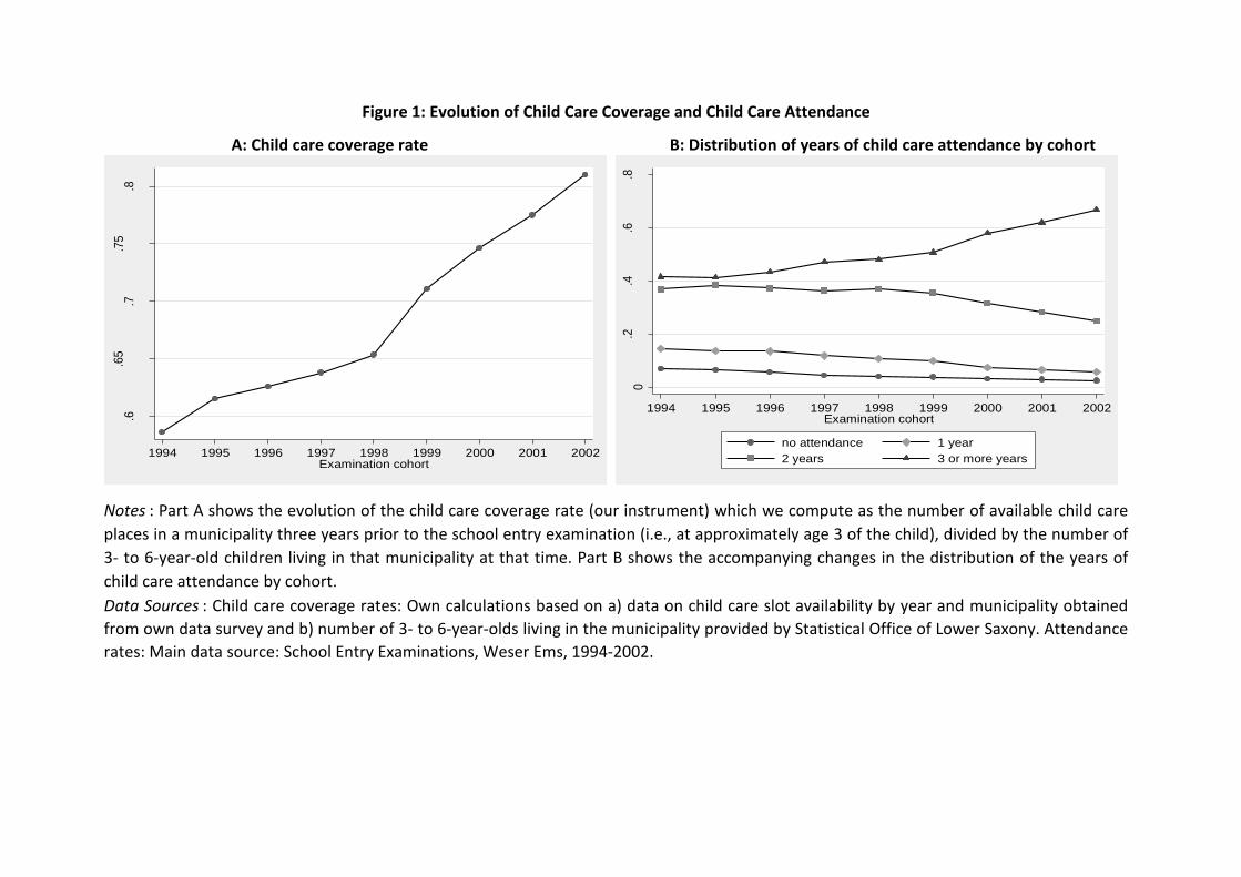
Figure 1: Evolution of Child Care Coverage and Child Care Attendance

A: Child care coverage rate B: Distribution of years of child care attendance by cohort

Notes : Part A shows the evolution of the child care coverage rate (our instrument) which we compute as the number of available child care

places in a municipality three years prior to the school entry examination (i.e., at approximately age 3 of the child), divided by the number of

3- to 6-year-old children living in that municipality at that time. Part B shows the accompanying changes in the distribution of the years of

child care attendance by cohort.

Data Sources : Child care coverage rates: Own calculations based on a) data on child care slot availability by year and municipality obtained

from own data survey and b) number of 3- to 6-year-olds living in the municipality provided by Statistical Office of Lower Saxony. Attendance

rates: Main data source: School Entry Examinations, Weser Ems, 1994-2002.

.6.6

5.7

.75

.8

Child

ca

re c

ove

rag

e r

ate

1994 1995 1996 1997 1998 1999 2000 2001 2002Examination cohort

0.2

.4.6

.8

1994 1995 1996 1997 1998 1999 2000 2001 2002Examination cohort

no attendance 1 year

2 years 3 or more years

Notes : The graph displays, based on the same specification as in Column (1) of Table 4, the propensity

score predicted from a probit regression as a function of the child care coverage rate (Z) by minority status

and gender, holding all other control variables at mean values.

Figure 2: The propensity score P(Z) as a function of the child care coverage rate (Z) by gender and

minority status

Main data source: School Entry Examinations, Weser Ems, 1994-2002.

0.2

.4.6

P(Z

)

.2 .4 .6 .8 1Z

Majority, male Majority, female

Minority, male Minority, female

Main data source: School Entry Examinations, Weser Ems, 1994-2002.

Notes : The figure plots the frequency distribution of the propensity score by

treatment status. The propensity score is predicted from the baseline first-

stage regression in Column (1) of Table 4.

Figure 3: Common Support

Main data source : School Entry Examinations, Weser Ems, 1994-2002.

A: MTE curve at average values of the covariates

B: MTE curves and weights for the treated and untreated

C: MTE curve and weights for individuals shifted by the instrument

Notes: Part A depicts the MTE curve for school readiness based on the specification in Columns (1) and (2) in Table 4 and

evaluated at mean values of the covariates. The 90% confidence interval is based on bootstrapped standard errors clustered at

the municipality level. Part B displays the MTE curves evaluated at covariate means for treated and untreated individuals, and

the associated weights to compute the treatment effects on the treated and on the untreated (see Section 4.4 in Cornelissen et

al., 2016). Part C plots the MTE curve evaluated at covariate means of those children who are shifted into early child care in

response to changes in the instrument, and the associated weights to compute the IV effect (see Appendix C in Cornelissen et

al., 2016). The two horizontal lines refer to the IV (2SLS) effect estimated from our data (dashed line) and aggregated over the

MTE curve (dotted line).

Figure 4: MTE curves for School Readiness

0.0

05

.01

.01

5.0

2

-.2

-.1

0.1

.2.3

0 .2 .4 .6 .8 1U_D

MTE at X of treated MTE at X of untreated

TT weights TUT weights

-.4

-.2

0.2

.4

0 .2 .4 .6 .8 1U_D

MTE 90% CI

Estimated Marginal Treatment Effects

0.0

05

.01

.01

5.0

2

IV w

eig

hts

-.1

0.1

.2.3

0 .2 .4 .6 .8 1U_D

MTE at X of compliers 2SLS estimate (.07)

IV weights Weighted MTE (.06)

Main data source : School Entry Examinations, Weser Ems, 1994-2002.

Figure 5: MTE curves - functional form robustness checks

Notes : The figure displays MTE curves for the outcome of school readiness, evaluated at mean values of the

covariates. The solid MTE curve refers to our baseline specification where the propensity score and its square is

included in equation (4), implying a linear MTE curve. The figure also shows three additional MTE curves which

allow for richer patterns such as a U-shaped MTE curve: one curve obtained from a semiparametric approach, and

two curves based on specifications which include a cubic and quartic of the propensity score in equation (4).

-.4

-.2

0.2

.4

0 .2 .4 .6 .8 1U_D

Baseline Third order polynomial

Semiparametric Fourth order polynomial

Main data source : School Entry Examinations, Weser Ems, 1994-2002.

Figure 6: MTE curves from ordered selection model for one, two and three years of child care

Notes: The figure displays separate MTE curves for the effects of moving from 1 year of child care to 2

years of child care (solid line) and moving from 2 years of child care to 3 years (dashed line) for the

outcome of school readiness based on a normal selection model with a generalized ordered probit

selection equation (see Appendix B for a description of that model). The curves are evaluated at mean

values of the covariates. Both curves are statistically significantly upward sloping pointing towards a

selection pattern of reverse selection on gains.

-.1

-.05

0

.05

.1.1

5

0 .2 .4 .6 .8 1U_D

Ordered Normal 2 vs 1 Ordered Normal 3 vs 2

Main data source : School Entry Examinations, Weser Ems, 1994-2002.

Notes : Part A plots, for our main outcome of school readiness, the unobserved component of the outcome against

the unobserved resistance to treatment U_D, separately for the treated (i.e., E(U_1 |U_D=u_D ), solid line) and

untreated (i.e., E(U_0 |U_D=u_D ), dashed line) state, following Brinch, Mogstad and Wiswall (2016). Panels B to F

repeat the exercise, but use indicator variables for: whether the child attended the first four routine postnatal

medical checkups before entry into child care (Part B); whether the postnatal checkup book is present at the

examination (Part C); whether the mother or father hold a college degree (Panels D and E); and whether the child is

a single child (Part F) as dependent variables, to learn about how families with a low resistance to enroll their child in

early child care differ from families with a high resistance.

Figure 7: Unobserved component of outcomes as a function of resistance

to treatment, by treatment state

A: School Readiness B: Attendance at routine postnatal checkups

D: College degree mother

E: College degree father F: Only child

C: Postnatal checkup book present

-.05

0

.05

0 .2 .4 .6 .8 1U_D

Untreated Treated

-.4

-.2

0.2

.4

0 .2 .4 .6 .8 1U_D

Untreated Treated

-.4

-.2

0.2

.4

0 .2 .4 .6 .8 1U_D

Untreated Treated

-.4

-.2

0.2

.4

0 .2 .4 .6 .8 1U_D

Untreated Treated

-.15

-.1

-.05

0

.05

.1

0 .2 .4 .6 .8 1U_D

Untreated Treated

-.1

-.05

0

.05

.1

0 .2 .4 .6 .8 1U_D

Untreated Treated

Treatment variable

Child care attendance for at least 3 years 0.51

Selected Covariates

Minority 0.12

Female 0.49

Age at examination in months 74.68

Outcomes

School Readiness 0.91

Predicted School Readiness

Minimum 0.31

5th percentile 0.74

10th percentile 0.79

25th percentile 0.87

50th percentile 0.93

75th percentile 0.97

90th percentile 0.98

Motor Skills 0.85

No Compensatory Sport Required 0.82

BMI 15.61

Overweight (BMI > 90th percentile) 0.08

Mother has no post-secondary education

Majority (German origin) 0.07

former Soviet Union (35% of minority children) 0.28

Turkish (31% of minority children) 0.57

Mother has college degree

Majority (German origin) 0.37

former Soviet Union 0.34

Turkish 0.15

former Soviet Union 0.44

Turkish 0.38

Child to staff ratio (median) 9.44

Share of high educated among staff 0.09

Share of male staff 0.02

Data Sources : Panel A: School Entry Examinations, Weser Ems, 1994-2002. Panel B: School Entry

Examinations, Weser Ems, 2001-2003 and information of German spoken with at least one family

member (father, mother or grandparents) from the Special Survey on Russian and Turkish children for

Children Longitudinal Study from the German Youth Institute (DJI), Munich, 2003. The sample refers to

8- and 9-year old children of former Soviet Union (N=262) and of Turkish origin (N=256) in 2003. Panel

C: Social Security Records, Weser-Ems, 1990-1998, 18-65 year olds.

Panel A: Individual characteristics

Panel C: Child care quality indicators

Table 1: Descriptive statistics

Notes: Panel A reports sample means of early child care attendance (our treatment variable),

of selected child characteristics, and of child outcomes in our sample. Panel B compares

sample means of maternal education between majority children and children of Turkish origin

and from the Soviet Union. In addition it reports the share of children of Turkish origin and

from the Soviet Union origin who speak primarily German with at least one family member,

based on data from the Children Longitudinal Survey. Panel C displays sample means of child

care quality indicators at the municipality level, referring to when the child was 3 years old.

Panel B: Characteristics of minority / majority groups

German spoken with at least one family member (Family Survey)

(1) (2)

Initial coverage rate -0.437** -0.478**

(0.175) (0.190)

Median wage level 0.000

(0.002)

Share of high educated 0.010

(0.011)

Share of medium educated 0.003

(0.003)

Number of inhabitants in 1000 0.0001

(0.000)

Share of immigrants in workforce 0.014**

(0.007)

Share of women in workforce -0.0002

(0.002)

Constant 0.172*** 0.202***

(0.016) (0.026)

p-value for joint significance of other covariates

(excluding initial coverage rate)0.1855

Table 2: Determinants of the child care expansion

Notes: The table investigates the determinants of the expansion in child care slots in

the municipality, by regressing the change in the child care coverage rate in the

municipality between examination cohorts 1994 and 2001 on the initial coverage rate

for the 1994 cohort (Column (1)), and baseline municipality characteristics (Column (2)).

The child care coverage rate is measured 3 years prior to the school entry examination

(i.e., when the cohort is approximately aged 3). In municipalities where information for

1994 or 2001 was missing, we use the adjacent cohort. The last row reports the p-value

for the hypothesis that municipality characteristics at baseline are jointly equal to zero.

All coefficients on shares refer to one-percentage point changes in these shares.

Bootstrapped standard errors clustered at the municipality level are reported in

parentheses. *Statistically significant at 0.10 level, ** at 0.05 level, *** at 0.01 level.

Data Sources : Child care coverage rates: Own calculations based on a) data on child

care slot availability by year and municipality obtained from own data survey and b)

number of 3-6 year olds living in the municipality provided by Statistical Office of Lower

Saxony. Median wage, educational shares, share of immigrants and women in

workforce: Social Security Records, Weser-Ems, 1990-1998, 18-65 year olds. Number of

inhabitants: Statistical Office of Lower Saxony.

child care coverage rate

Age -0.00001

(0.0001)

Age Squared 0.0000

(0.0020)

Female -0.0003

(0.0002)

Minority child -0.00003

(0.0005)

Median wage level 0.002

(0.001)

Share of high educated 0.009

(0.011)

Share of medium educated -0.002

(0.002)

Number of inhabitants in 1000 0.000

(0.003)

Share of immigrants in workforce 0.003

(0.006)

Share of women working 0.004

(0.003)

Municipality dummies Yes

Cohort dummies Yes

p-value for joint significance of covariates 0.254

Table 3: Balancing tests

Notes: The table reports coefficients from regressions of the instrument (the

child care coverage rate) on individual and municipality-level covariates

measured in the previous period, conditional on municipality and cohort

dummies. The child care coverage rate is measured 3 years prior to the school

entry examination (i.e., when the cohort is approximately aged 3). The last

row reports the p-value for the hypothesis that the covariates are jointly

equal to zero. All coefficients on shares refer to one-percentage point changes

in these shares. Bootstrapped standard errors clustered at the municipality

level are reported in parentheses. *Statistically significant at 0.10 level, ** at

0.05 level, *** at 0.01 level.

Data sources : Child care coverage rates: Own calculations based on a) data on

child care slot availability by year and municipality obtained from own data

survey and b) number of 3-6 year olds living in the municipality provided by

Statistical Office of Lower Saxony. Individual characteristics: School Entry

Examinations, Weser Ems, 1994-2002. Median wage, educational shares,

share of immigrants and women in workforce: Social Security Records, Weser-

Ems, 1990-1998, 18-65 year olds. Number of inhabitants: Statistical Office of

Lower Saxony.

Selection Eq. Outcome Eq. Selection Eq. Outcome Eq.

Child care

>=3 years

School

Readiness

Child care

>=3 years

School

Readiness

(1) (2) (3) (4)

Child care coverage rate 0.331*** 0.331***

(0.043) (0.042)

Child care coverage rate squared -0.220** -0.220**

(0.108) (0.108)

Female 0.014*** 0.092*** 0.014*** 0.092***

(0.003) (0.009) (0.003) (0.009)

Minority -0.198*** -0.120***

(0.011) (0.020)

Turkish -0.207*** -0.199***

(0.019) (0.031)

Ethnic Germans (Former Soviet Union) -0.213*** -0.073***

(0.015) (0.024)

Other Minorities -0.178*** -0.144***

(0.010) (0.028)

Propensity Score -0.135 -0.170

(0.115) (0.131)

Propensity Score squared 0.215** 0.205*

(0.099) (0.105)

Female * Propensity Score -0.086*** -0.085***

(0.014) (0.015)

Minority * Propensity Score 0.117***

(0.035)

Turkish * Propensity Score 0.201***

(0.065)

Ethnic Germans (Former Soviet Union) * 0.063

Propensity Score (0.043)

Other Minority * Propensity Score 0.143***

(0.041)

Chi-squared for test of excluded instruments 56.83 72.71

p-value for test of excluded instruments 0.0000 0.0000

p-value for test of heterogeneity 0.029 0.051

N 135,906 135,906 135,906 135,906

Main data source : School Entry Examinations, Weser Ems, 1994-2002.

Notes: Columns (1) and (3) report average marginal effects from probit selection models where the

dependent variable is equal to 1 if the child attends public child care for at least three years (“first

stage”). The child care coverage rate (our instrument) is measured relative to its overall mean. The

instrument in the probit selection equation is interacted with individual characteristics (age, gender,

ethnic minority status); interaction terms are not shown to save space, but the heterogeneous effect by

minority status and gender is depicted in Figure 2. The coefficients on the child care coverage rate refer

to a German boy of average age. Columns (2) and (4) display estimates from the outcome equation (see

equation (4) in the text) where the dependent variable is an indicator variable for school readiness.

Coefficients of regressors not interacted with the propensity score measure effects on the outcome in

the untreated state (i.e., β0 in equation (4)), whereas coefficients of regressors interacted with the

propensity score measure the difference of the effects between the treated and the untreated state (β1-

β0 in equation (4)). In columns (3) and (4) we further allow the effects of early child care attendance to

differ between the two main minority groups in our sample: children of Turkish descent and children

from the former Soviet Union. Further included controls not displayed in the table are age and age

squared and time-varying municipality sociodemographic characteristics in t-4 as well as child care

quality indicators in t-3, each interacted with the propensity score, as well as cohort dummies,

municipality dummies and birth month dummies (not interacted with the propensity score).

Bootstrapped standard errors clustered at the municipality level are reported in parentheses.

*Statistically significant at 0.10 level, ** at 0.05 level, *** at 0.01 level.

Table 4: Selection Equation and School Readiness Outcome Equation

(1) (2) (3) (4) (5) (6) (7) (8)

BaselineNon-

interacted

Non-

interacted,

linear

Initial coverage

rate IV

Long

difference

Birth months

Jan - JunAge dummies

No quality

controls

ATE 0.059 0.050 0.045 0.130 -0.005 0.114 0.048 0.073

(0.072) (0.069) (0.072) (0.105) (0.084) (0.092) (0.073) (0.072)

TT -0.051 -0.070 -0.071 0.008 -0.152 -0.020 -0.053 -0.072

(0.080) (0.085) (0.092) (0.109) (0.118) (0.128) (0.084) (0.082)

TUT 0.173** 0.176** 0.165** 0.251** 0.160 0.219** 0.154* 0.223***

(0.085) (0.083) (0.082) (0.120) (0.113) (0.106) (0.093) (0.082)

p-value for test of

heterogeneity0.029 0.031 0.054 0.028 0.074 0.119 0.092 0.008

N 135,906 135,906 135,906 146,522 56,942 66,865 135,906 135,906

Main data source : School Entry Examinations, Weser Ems, 1994-2002.

Table 5: Robustness checks

Notes: The table reports, for our main outcome variable of school readiness, the average treatment effect (ATE), the treatment effect on

the treated (TT), treatment effect on the untreated (TUT) and the p-value for a test of essential heterogeneity for various alternative

specifications. Column (1) refers to the baseline regression from column (2) in Table 4. In column (2), the instrument is not interacted with

covariates in the selection equation, and in column (3) the instrument is not interacted and the quadratic term of the instrument is

dropped. In Column (4), the instrument is the initial child care coverage rate (for the oldest cohort in our data) interacted with cohort

dummies (and gender, minority status and age, as in our baseline specification). Column (5) only exploits variation across municipalities in

the intensity of the child care expansion and restricts the analysis to the (pooled) oldest and youngest examination cohorts 1994/95 vs.

2001/02. In Column (6), the sample is restricted to children born in the first half of the calendar year, and in Column (7), monthly age

dummies instead of a quadratic in age are included as controls. In Column (8), child care quality controls are not included in the

regressions. The reported p-value for a test of heterogeneity is a test for a non-zero slope of the MTE curve (see also Section 2.2).

Bootstrapped standard errors clustered at the municipality level are reported in parentheses. *Statistically significant at 0.10 level, ** at

0.05 level, *** at 0.01 level.

School Readiness

(i) Female 0.081***

(0.0095)

(ii) Minority -0.107***

(0.0268)

(iii) Childcare >= 2 * Female -0.023***

(0.0084)

(iv) Childcare >= 2 * Minority 0.042**

(0.0163)

(v) Childcare >= 3 * Female -0.020***

(0.0046)

(vi) Childcare >= 3 * Minority 0.046***

(0.0097)

Test for upward sloping MTE curves

(vii) ρ3 -ρ2 0.030**

(0.0120)

(viii) ρ2 -ρ1 0.046**

(0.0194)

Implied ATE

(ix) 2 versus 1 years 0.0098

(0.0453)

(x) 3 versus 2 years 0.0574

(0.0386)

Notes: The table presents results from the outcome equation of a generalized normal ordered choice roy model,

modelling three treatment states (attending child care for less than 2 years, for 2 years, or for 3 years or more).

The model is described in more detail in Appendix B, and the first stage results are shown in Appendix Table A1 of

Appendix A. The outcome equation is estimated by including Heckman-type selection correction terms for all

three treatment states generated from the first stage model and by interacting all covariates with dummies for at

least 2 years and at least 3 years of child care. For minority children, for example, the coefficients on the

interaction terms Childcare >= 2 * Minority and Childcare >= 3 * Minority in Rows (iv) and (vi) show that minority

children have a higher treatment effect for both moving from 1-2 years of child care and moving from 2-3 years of

child care. ρ1, ρ2, and ρ3 are the correlations of the outcome error terms in each of the three states (U1, U2, and

U3) with the error term of the selection equation V. The differences ρ3 -ρ2 and ρ2 -ρ1 are reported in Rows (vii)

and (viii) of the table and are informative on the pattern of selection, with positive values for the difference

indicating reverse selection on gains (a rising MTE curve). Transition-specific ATEs (at mean values of covariates)

are reported in rows (ix) and (x) in the table, and the corresponding transition-specific MTE curves are depicted in

Figure 6. Bootstrapped standard errors clustered at the municipality level are reported in parentheses.

*Statistically significant at 0.10 level, ** at 0.05 level, *** at 0.01 level. Number of observations: 131,845.

Main data source : School Entry Examinations, Weser Ems, 1994-2002.

Table 6: Outcome equation of generalized normal ordered choice roy model

School

Readiness

Motor

Skills

No

Compensatory

Sport

Overweight Log BMI

Panel A: Conventional Treatment Effects

ATE 0.059 0.018 0.203** 0.017 0.025

(0.072) (0.088) (0.092) (0.034) (0.023)

TT -0.051 0.001 0.099 0.052 0.045

(0.080) (0.118) (0.119) (0.045) (0.028)

TUT 0.173** 0.035 0.308*** -0.019 0.003

(0.085) (0.103) (0.115) (0.037) (0.027)

p-value for test of heterogeneity 0.029 0.767 0.214 0.071 0.152

Panel B: Effects of child care quality characteristics

Above-median child to staff ratio 0.005 0.041 -0.044 -0.016 -0.008

* Propensity Score (0.031) (0.034) (0.045) (0.019) (0.010)

Share of high educated among staff 0.025 0.465* -0.229 -0.003 0.035

* Propensity Score (0.258) (0.267) (0.406) (0.113) (0.075)

Share of male staff * Male child 0.013** 0.028*** 0.033** -0.008** -0.005**

* Propensity Score (0.007) (0.007) (0.014) (0.004) (0.002)

Share of male staff * Female child 0.008 0.015** 0.009 -0.009*** -0.006***

* Propensity Score (0.007) (0.008) (0.012) (0.003) (0.002)

Main data source : School Entry Examinations, Weser Ems, 1994-2002.

Table 7: Other Outcomes

Notes: Panel A reports the average treatment effect (ATE), the treatment effect on the treated (TT),

treatment effect on the untreated (TUT) and the p-value for a test of essential heterogeneity for

five outcomes: our main outcome of school readiness; no motor skill problems; no compensatory

sport required; overweight, measured as the BMI above the (age- and gender-specific) 90th

percentile; and the log BMI. Panel B displays coefficient estimates of the interaction terms between

child care quality indicators and the propensity score; these terms measure how child care quality

influences the returns to early child care attendance. Further included controls not displayed in the

table are age and age squared and time-varying municipality sociodemographic characteristics as

well as child care quality indicators (interacted with the propensity score) as well as cohort

dummies, municipality dummies and birth month dummies (not interacted with the propensity

score). Coefficients on the interaction terms of share of male staff refer to a one-percentage point

change in this share. Bootstrapped standard errors clustered at the municipality level are reported

in parentheses. *Statistically significant at 0.10 level, ** at 0.05 level, *** at 0.01 level.

1994 2000

public child care 41.2% 75.8%

only family care (parents and other relatives) 58.3% 22.7%

exclusively maternal care 39.3% 18.8%

informal care (nanny, other non-relatives) 1.2% 1.5%

Maternal labour force participation (3-year-olds) 31.2% 38.7%

public child care, children of working mothers 42.9% 81.5%

public child care, children of non-working mothers 40.5% 72.2%

Table 8: Child care arrangements for 3-year-olds, 1994 and 2000

Notes : The table provides, for the years 1994 and 2000, information on child care

arrangements of 3-year-olds, distinguishing between public child care; only family care by

parents or grandparents; only maternal care; and care by a child-minder or nanny. The table

also reports labor force participation rates of mothers of 3-year-olds, as well as public child

care attendance rates of 3-year-olds separately by the mother’s labor force status.

Data source : Own calculation based on Family Survey from the German Youth Institute (DJI),

Munich, 2nd and 3rd wave (1994 and 2000). The sample refers to 3-year-olds in West

Germany and consists of 262 children in 1994 and 354 children in 2000.

(1) (2) (3)

PRTE Baseline Policy

(i) Bring 2002 P(Z) to .9 by adding .275 0.160* 0.67 0.90

(0.085)

(ii) Bring 2002 P(Z) to .9 by multiplying 1.5 0.165* 0.67 0.90

(0.087)

(iii) Lift 2002 cohort's coverage rate (Z) to 1 if <1 0.123 0.67 0.71

(0.077)

(iv) Add 0.4 to 2002 cohort's coverage rate (Z) 0.141* 0.67 0.72

(0.086)

Main data source : School Entry Examinations, Weser Ems, 1994-2002.

Propensity score

Table 9: Policy-relevant treatment effects

Notes: The table reports in Column (1) policy-relevant treatment effects (PRTE) per net child shifted for four

different policies. In Rows (i) and (ii), we simulate a policy which brings the average early attendance rate (or

equivalently the propensity score) from its 2002 level of .67 to a level of .9, by adding a constant of 0.275 to

each child’s 2002 propensity score (Row (i)), or by multiplying each child’s 2002 propensity score by a constant

of 1.5 (Row (ii)). In Rows (iii) and (iv), we instead directly manipulate the 2002 cohort's child care coverage rate

(i.e., the coverage rate measured in 1999, when the 2002 cohort was 3 years old–our instrument). In Row (iii),

we set the coverage rate to 1 for municipalities in which it is below 1; in Row (iv), we instead add a constant of

0.4 to the coverage rate, allowing for coverage rates greater than 1 in some municipalities. Columns (2) and (3)

show the increase in the propensity score which each policy induces. Estimates refer to our baseline

specification displayed in Columns (1) and (2) of Table 4 and Panel A of Figure 4. Bootstrapped standard errors

clustered at the municipality level are reported in parentheses. *Statistically significant at 0.10 level, ** at 0.05

level, *** at 0.01 level.