Who Is (More) Rational?∗

Syngjoo Choi, Shachar Kariv, Wieland Müller, and Dan Silverman†

August 9, 2013

Abstract

Revealed preference theory offers a criterion for decision-making

quality: if decisions are high quality then there exists a utility func-

tion the choices maximize. We conduct a large-scale experiment to

test for consistency with utility maximization. Consistency scores

vary markedly within and across socioeconomic groups. In particu-

lar, consistency is strongly related to wealth: a standard deviation

increase in consistency is associated with 15-19 percent more house-

hold wealth. This association is quantitatively robust to conditioning

on correlates of unobserved constraints, preferences, and beliefs. Con-

sistency with utility maximization under laboratory conditions thus

captures decision-making ability that applies across domains and in-

fluences important real-world outcomes.

∗We thank Douglas Gale and Raymond Fisman for detailed comments and sugges-tions. We are also grateful to James Andreoni, James Banks, Richard Blundell, Andrew

Caplin, David Card, Thomas Crossley, Stefano DellaVigna, Guillaume Frechette, Stef-

fen Huck, Patrick Kline, Ron Lee, John List, Nicola Persico, Imran Rasul, Joel Slemrod

and Hans-Martin von Gaudecker for helpful discussions and comments. This paper has

also benefited from suggestions by the participants of seminars at several universities

and conferences. Jelmer Ypma provided excellent research assistance. We thank Cor-

rie Vis and Edwin de Vet of CentERdata (Tilburg University) for software development

and technical support. We acknowledge financial support from the Economic and So-

cial Research Council (ESRC) Grant No. RES-061-25-0348 (Choi); the National Science

Foundation (SES-0962543), the Multidisciplinary University Research Initiative (MURI),

and the Center on the Economics and Demography of Aging (CEDA) and the Coleman

Fung Risk Management Research Center (OpenLink Fund) at UC Berkeley (Kariv); and

the Netherlands Organisation for Scientific Research (NWO) and the Network for Studies

on Pensions, Aging and Retirement (Netspar) (Müller).†Choi: University College London (email: syngjoo.choi@ucl.ac.uk); Kariv: Univer-

sity of California—Berkeley (email: kariv@berkeley.edu); Müller: University of Vienna and

Tilburg University (email: wieland.mueller@univie.ac.at); Silverman: University of Michi-

gan and NBER (email: dansilv@umich.edu).

1

JEL Classification Numbers: C93, D01, D03, D12, D81

Keywords: Decision-making quality, rationality, revealed prefer-

ence, risk, wealth differentials, Netherlands, experiment, CentERpanel.

1 Introduction

In his Foundations of Economic Analysis (1947), Paul Samuelson offered

a natural criterion for decision-making quality based solely on observable

behavior. Adopting Samuelson’s approach, we test whether individual be-

havior in a choice under risk experiment is consistent with the utility max-

imization model. We conducted the experiment using the CentERpanel, a

panel study of a large representative sample of households in the Netherlands

that collects a wide range of individual sociodemographic and economic in-

formation about its members.

The paper provides three types of analysis. First we offer a purely de-

scriptive overview of the consistency of the experimental data with the util-

ity maximization model. Second we analyze the correlation between the

levels of consistency and socioeconomic characteristics. In this way we ad-

dress the question: “who is (more) rational?” Third, we test the validity

of a causal interpretation of the relationship between our proposed measure

of decision-making quality — the consistency of the experimental data with

utility maximization — and wealth accumulation in the real world.

In accordance with Samuelson’s approach, traditional economic analysis

assumes that individual behavior can be rationalized by a utility function.

In this standard view, heterogeneity in choices is attributed to heterogene-

ity in preferences, constraints, information, or beliefs. More recently, several

strands of research consider heterogeneity in choices driven also by differ-

ences in decision-making ability. Different from traditional analysis, this

literature allows that the choices that some people actually make may be

different from the choices they would make if they had the skills or knowledge

to make better decisions. This research thus takes the view that those with

lower decision-making ability may make choices of lower decision-making

quality.

The idea that people vary in their decision-making ability, and therefore

make choices of different decision-making quality, has intuitive appeal and

important consequences for economics. It is difficult, however, to make de-

finitive judgements about which choices exhibit low decision-making quality,

and which people have inferior decision-making ability, due to twin problems

of identification and measurement. The identification problem is to distin-

2

guish differences in decision-making ability from unobserved differences in

preferences, constraints, information, or beliefs. The measurement problem

is to define and implement a practical, portable, quantifiable, and econom-

ically interpretable measure of decision-making quality. The two problems

are conceptually distinct, but tightly linked in practice.

The identification problem emerges because it is usually unclear whether

those with lower decision-making ability — as evidenced by less education,

lower cognitive abilities, or less financial literacy — are making choices of

lower decision-making quality. They might have different preferences over

the same outcomes, or face different but unobserved incentives and con-

straints, or have different information, or hold different beliefs. The mea-

surement problem emerges because only rarely are the relevant incentives

so clear and the data quality so high, that classifying some choices as of low

decision-making quality is straightforward and uncontroversial. Typically,

a measure of decision-making quality is challenging to formalize, quantify,

and make practical for application in a variety of choice environments.

We offer a new approach to the challenges posed by the identification

and measurement problems. Our point of departure is a proposal to mea-

sure decision-making quality by the consistency of choices with economic

rationality, in the sense of a complete and transitive preference ordering.

Adopting this standard for decision-making quality, we present individuals

with an economic choice experiment which provides a stringent test of utility

maximization. The measure thus has a well-established economic interpre-

tation and revealed preference theory tells us whether we have enough data

to make it statistically useful. In addition, the analytical techniques and

experimental platform are easily portable to a variety of choice problems.

Our approach thus addresses the measurement problem.

Furthermore, an experiment like ours, to the extent possible, holds in-

formation and beliefs constant within subject, and controls the relevant

constraints. If decision-making ability is defined simply as the capacity to

make choices of higher decision-making quality, then our approach addresses

the identification problem inside the laboratory. It can distinguish individ-

ual heterogeneity in decision-making ability from unobserved differences in

preferences, constraints, information, or beliefs.

Our interest in decision-making quality under laboratory conditions largely

derives, however, from the possibility that it reflects decision-making ability

that affects important outcomes outside the laboratory. We evaluate this

possibility first by examining the correlation between decision-making qual-

ity in the experiment and socioeconomic characteristics. The goal of this

analysis is not to establish causation. If, however, we find a significant cor-

3

relation between decision-making quality and certain characteristics, this

lends a basic level of credence to the idea that people with these charac-

teristics tend to make different choices not just because they face different

constraints or have different preferences, but also because they tend to have

different levels of decision-making ability.

To evaluate a causal interpretation of the link between decision-making

quality in the experiment and important economic outcomes in the real

world, we examine whether our measure of decision-making quality from

the experiment can independently and robustly explain real-world economic

outcomes, conditional on socioeconomic characteristics including income,

age, education and occupation. If heterogeneity in decision-making ability is

an important source of heterogeneity in real world outcomes, and if decision-

making quality in the experiment is a good proxy for decision-making ability,

then differences in the experiment-based measure across subjects should help

explain differences in their real-world outcomes.

We chose wealth as the outcome of interest because the task of explaining

wealth provides a strong test of the idea that decision-making quality in the

experiment reflects a more general form of decision-making ability. The test

is strong because wealth is determined by countless decisions, made over

time in many different settings, and involving many different tradeoffs, thus

increasing our chance of rejecting a relationship. We are also motivated

to study wealth by prior research that documents large wealth differentials

among households with similar life-time income. The extent to which these

differentials can be explained either by standard observables, such as family

structure or income volatility, or by standard unobservables, such as risk

tolerance or intertemporal substitution, is a subject of some debate (see,

Bernheim et al., 2001, Ameriks et al., 2003, and Scholz et al., 2006, for

different perspectives).

A causal interpretation of the relationship between decision-making qual-

ity in the experiment and wealth depends importantly on the estimated

correlation between these two measures being quantitatively robust to con-

ditioning on additional correlates of unobserved preferences, constraints,

information, and beliefs. This assessment of robustness is not an effort to

“control for everything.” Instead, in the spirit of Altonji et al. (2005), we

examine whether the estimated correlation is much affected by the inclusion

of additional controls that, a priori, should be correlated with economic out-

comes through their correlation with unobserved or misspecified variables.

If these unobservables are indeed important sources of the observed correla-

tion between consistency and economic outcomes, then adding the controls

should have a substantial effect on the estimated correlation coefficients.

4

We measure the decision-making quality in the experiment by evaluat-

ing the consistency of individual behaviors with the Generalized Axiom of

Revealed Preference (GARP). We assess how nearly individual choice behav-

ior complies with GARP using standard measures of consistency that have

been proposed for quantifying the extent of violations. There is consider-

able heterogeneity within and across sociodemographic categories. Taking

advantage of the large and heterogeneous CentERpanel sample, we find

that high-income and high-education subjects display greater levels of con-

sistency than lower-income and lower-education subjects. In addition, men

are more consistent than women, and young subjects tend more toward

utility maximization than those who are old. The magnitudes imply that

low-income subjects on average “leave on the table” as much as 3.3 per-

centage points more of their earnings, relative to high-income subjects, by

making inconsistent choices. The corresponding numbers for low-education

subjects, females, and old subjects are 2.6, 2.4, and 5.1, respectively.

We also find an economically large and statistically significant correla-

tion between consistency in the experiment and household wealth. The point

estimates indicate that, conditional on measures of current income, age, edu-

cation, occupation, basic demographic characteristics, and household struc-

ture, a standard deviation increase in the consistency score of the person

who is primarily responsible for household financial matters is associated

with 15-19 percent more household wealth. As important, this estimated

correlation is quantitatively robust to conditioning on many additional cor-

relates of unobserved preferences, constraints, information, and beliefs. We

interpret the economically large, statistically significant, and quantitatively

robust relationship between decision-making quality in the experiment — the

consistency of the experimental data with the utility maximization model

— and household wealth as evidence of decision-making ability that applies

across choice domains and affects important real-world outcomes.

We also show that alternative measures of decision-making quality from

the experiment and decision-making ability from the CentERpanel survey

are not substitutes for our measure of compliance with GARP. The alterna-

tives include (i) a stronger notion of decision-making quality in our experi-

ment that measures the extent of violations of both GARP and first-order

stochastic dominance, (ii) parametric estimates of a tendency to “tremble”

in an experiment by von Gaudecker et al. (2011) with an overlapping sample

of CentERpanel members, and (iii) scores from Frederick’s (2005) Cognitive

Reflection Test that, in other samples, is well-correlated with measures of

cognitive ability. We find that these three alternatives either have no inde-

pendent power to predict wealth, or are not well-correlated with compliance

5

with GARP in the experiment. Finally, we investigate the correlation be-

tween decision-making quality in the experiment and details of household

saving allocations that influence wealth.

The rest of the paper is organized as follows. Section 2 describes the

experimental design and procedures. Section 3 describes decision-making

quality in the experimental data. Section 4 contains analysis of the cor-

relation between decision-making quality and socioeconomic characteristics.

Section 5 discusses the relationship between wealth differentials and decision-

making ability. Section 6 describes the margins along which we extend the

previous literature. Section 7 contains some concluding remarks. The paper

also includes six data and technical appendices for the interested reader.1

2 The experiment

2.1 Sample

The experiment uses the CentERpanel, an online, weekly, and stratified

survey of a sample of over 2,000 households and 5,000 individual members.

The sample is designed to be representative of the Dutch-speaking popu-

lation in the Netherlands. Via the Internet, the survey instrument allows

researchers to implement experiments and collects a great deal of individual

demographic and economic information from its respondents. The subjects

in the experiment were recruited at random from the entire CentERpanel

sample. The experiment was conducted online with 1,182 CentERpanel

adult members. Table 1 provides summary statistics of individual charac-

teristics. We present the data for participants (completed the experiment),

dropouts (logged in but quit the experiment) and nonparticipants (recruited

for the experiment but never logged in). In later analysis we will control for

sample selection using Heckman’s (1979) model.

[Table 1 here]

2.2 Design

In our experiment, we present subjects with a sequence of decision prob-

lems under risk. Each decision problem was presented as a choice from a

two-dimensional budget line. A choice of the allocation from the budget line

represents an allocation of points between accounts and (corresponding

to the horizontal and vertical axes). The actual payoffs of a particular choice

1Appendix #: http://emlab.berkeley.edu/~kariv/CKMS_I_A#.pdf.

6

were determined by the allocation to the and accounts; the subject re-

ceived the points allocated to one of the accounts or , determined at

random and equally likely. An example of a budget line defined in this way

is the line drawn in Figure 1. The point , which lies on the 45 de-

gree line, corresponds to the equal allocation with certain outcome, whereas

point and represent allocations in which all points are allocated to one

of the accounts. Notice that points along are risky — they have a lower

payoff in state and a higher payoff in state — but because the slope of

the budget line is steeper than −1, they have higher expected returnthan point . By contrast, points along have lower expected return

than point .

[Figure 1 here]

2.3 Procedures

The procedures described below are identical to those used by Choi et al.

(2007b), with the exception that the experiment described here consisted of

25, rather than 50, decision problems.2 We also made some minor changes

to accommodate the online experimental setting. Each decision problem

started with the computer selecting a budget line randomly from the set

of budget lines that intersect with at least one of the axes at 50 or more

points, but with no intercept exceeding 100 points. The budget lines selected

for each subject in different decision problems were independent of each

other and of the sets selected for any of the other subjects in their decision

problems. Choices were restricted to allocations on the budget constraint.3

Choices were made using the computer mouse to move the pointer on the

computer screen to the desired point and then clicking the mouse or hitting

the enter key. More information and full experimental instructions, including

the computer program dialog window, are available in Appendix I.

2The number of individual decisions is still higher than usual in the literature, and

revealed preference analysis presented below shows the experiment provides a data set

consisting of enough individual decisions over a sufficiently wide range of budget lines to

provide a powerful test of consistency.3Like Choi et al. (2007b), we restricted choices to allocations on the budget line so

that subjects could not dispose of payoffs. In Fisman et al. (2007), each decision involved

choosing a point on a graph representing a budget set that included interior allocations.

Since most of their subjects had no violations of budget balancedness (those who did

violate budget balancedness also had many GARP violations even among their choices

that were on the budget line), we restricted choices to allocations on the budget constraint

to make the computer program easier to use.

7

During the course of the experiment, subjects were not provided with

any information about the account that had been selected in each round.

At the end of the experiment, the computer selected one decision round for

each subject, where each round had an equal probability of being chosen,

and the subject was paid the amount he had earned in that round. Payoffs

were calculated in terms of points and then converted into euros. Each point

was worth 0.25. Subjects received their payment from the CentERpanel

reimbursement system via direct deposit into a bank account.

3 Decision-making quality

We propose to measure decision-making quality by the consistency of

choices with economic rationality, and we described a simple economic choice

experiment in which we can measure decision-making quality with a high

degree of precision, and separate it from other sources of heterogeneity in

choice. Specifically, we employ the GARP to test whether the finite set

of observed price and quantity data that our experiment generated may

be rationalized by a utility function. GARP generalizes various revealed

preference tests. It requires that if allocation is revealed preferred to

, then is not strictly and directly revealed preferred to ; that is,

allocation must cost at least as much as at the prices prevailing when

is chosen.4

If choices are generated by a non-satiated utility function, then the data

must satisfy GARP. Conversely, the result due to Afriat (1967) tells us that

if a finite data set generated by an individual’s choices satisfies GARP, then

the data can be rationalized by a utility function. Consistency with GARP

has long been a touchstone for rationality, but it demands only a complete

and transitive preference ordering. It places no restrictions on the utility

function, and makes no assumptions about what is reasonable to maximize.

Since it is possible to “pump” an indefinite amount of money out of an

individual making intransitive decisions, consistency with GARP provides a

crucial test of decision-making quality.

4Without loss of generality, assume the individual’s payout is normalized to 1. The

budget line is then 11 + 22 = 1 and the individual can choose any allocation that

satisfies this constraint. Let ( ) be the data generated by an individual’s choices, where

denotes the -th observation of the price vector and denotes the associated allocation.

An allocation is directly revealed preferred to if ≥ . An allocation is

revealed preferred to if there exists a sequence of allocations=1

with 1 = and

= , such that is directly revealed preferred to +1 for every = 1 − 1.

8

An individual’s decisions may violate GARP and thus be of low decision-

making quality for a number of reasons. First, violations of GARP can

result from “trembles.” Subjects may compute payoffs incorrectly, execute

intended choices incorrectly, or err in other less obvious ways. Second, in-

consistency can result from bounded rationality or cognitive biases such as

“framing effects” and “mental accounting” (Kahneman and Tversky, 1984).

The resources needed for determining optimal choices are limited. Thus,

especially in complex or unfamiliar environments, the cost of computing an

optimal decision can be high. Some subjects may therefore adopt simple

decision rules, and this “simplification” may cause their choices to be incon-

sistent.5 Third, if the data ( ) satisfy GARP, then they can be rational-

ized by an outcome-based utility function (1 2). However, unobserved

factors could enter the utility function so the “true” underlying preference

ordering is represented by a utility function (1 2 ) parametrized by .

If the data ( ) are generated by a utility function (1 2 ) and is

fixed, then the data will still satisfy GARP. An example of this is the disap-

pointment aversion model proposed by Gul (1991), where the safe allocation

1 = 2 is the reference point. If, however, is not fixed then subjects can

exhibit “preference reversals” and the data ( ) might not satisfy GARP

(cf. Bernheim and Rangel, 2009 where may be time). The variable may

also be interpreted, as in Koszegi and Rabin (2006), as a dynamic reference

point determined endogenously by the environment.

3.1 Consistency with GARP

Although testing conformity with GARP is conceptually straightforward,

there is a difficulty: GARP provides an exact test of utility maximization

— either the data satisfy GARP or they do not. We assess how nearly

individual choice behavior complies with GARP by using Afriat’s (1972)

Critical Cost Efficiency Index (CCEI), which measures the fraction by which

all budget constraints must be shifted in order to remove all violations of

GARP. Put precisely, for any number 0 ≤ ≤ 1, define the direct revealedpreference relation

() ⇔ · ≥ · 5Consistency is also endogenous: subjects can make decisions that are consistent with

GARP in a complex decision problem because they adopt simple choice rules to cope with

complexity. But in that case, the “revealed” preference ordering may not be the “true”

underlying preference ordering.

9

and define () to be the transitive closure of (). Let ∗ be the largestvalue of such that the relation () satisfies GARP. The CCEI is the ∗

associated with the data set.

Figure 2 illustrates the construction of the CCEI for a simple violation

of the GARP involving two allocations, 1 and 2. If we shift the budget

line through 1 as shown ( ) the violation would be removed

so the CCEI score associated with this violation is . By definition, the

CCEI is between zero and one — the closer the CCEI is to one, the smaller

the perturbation of the budget constraints required to remove all violations

and the closer the data are to satisfying GARP. The CCEI thus provides a

summary statistic of the overall consistency with GARP, reflecting the min-

imum adjustment required to eliminate all violations of GARP associated

with the data set.

[Figure 2 here]

In our experiment, the CCEI scores averaged 0.881, which implies that on

average budget lines needed to be reduced by about 12 percent to eliminate a

subject’s GARP violations.6 There is also marked heterogeneity in the CCEI

scores within and across socioeconomic groups. Figure 3 summarizes the

mean CCEI scores and 95 percent confidence intervals across selected socioe-

conomic categories. On average, high-income and high-education subjects

display greater levels of consistency than lower-income and lower-education

subjects. Men are more consistent than women, and young subjects tend

more toward utility maximization than those who are old. The magnitudes

imply that, in order to eliminate their GARP violations, low-income sub-

jects require an average contraction of their budgets that is 3.3 percentage

points larger than that of high-income subjects. The corresponding numbers

for low-education subjects, females, and old subjects are 2.6, 2.4, and 5.1,

respectively.7 We will further analyze the relationship between consistency

scores and socioeconomic characteristics, and address sample selection, in

our regression analysis below.

6 In contrast, Choi et al. (2007b) report that 60 of their 93 subjects (64.6 percent) had

CCEI scores above the 0.95 threshold and that over all subjects the CCEI scores averaged

0.954 (see Figure 1). The subjects of Choi et al. (2007b) were undergraduate students and

staff at UC Berkeley, and the experiment was conducted in the laboratory. We note that

the subjects of Choi et al. (2007b) were given a menu of 50 budget sets which provides a

more stringent test of GARP.7To allow for small trembles resulting from the slight imprecision of subjects’ handling

of the mouse, our consistency results allow for a narrow confidence interval of one point

(that is, for any and 6= , if −

≤ 1 then and are treated as the same

portfolio).

10

[Figure 3 here]

A key advantage of the CCEI is its tight connection to economic the-

ory. This connection makes the CCEI economically quantifiable and inter-

pretable. Moreover, the same economic theory that inspires the measure also

tells us when we have enough data to make it statistically useful. Thus this

theoretically grounded measure of decision-making quality helps us design

and interpret the experiments in several ways. In Appendix II, we provide

more details on testing for consistency with GARP, discuss the power of

the revealed preference tests, explain other indices that have been proposed

for this purpose, and describe the related empirical literature on revealed

preferences. In reporting our results, we focus on the CCEI. The results

based on alternative indices are presented in Appendix III. In practice, all

indices yield similar conclusions.

3.2 Beyond consistency

Stochastic dominance Consistency with GARP requires consistent pref-

erences over all possible alternatives, but any consistent preference ordering

is admissible. In this way, we see consistency as a necessary, but not suffi-

cient, condition for choices to be considered of high decision-making quality.

Indeed, choices can be consistent with GARP and yet fail to be reconciled

with any utility function that is normatively appealing. For example, con-

sider an individual who always allocates all points to the same account as

measured by 1. This behavior is consistent with maximizing the utility

function (1 2) = 1 and would generate a CCEI score of one.

Such preferences are, however, hard to justify in this setting because for

many of the budget lines that a subject faces, always allocating all points to

the same account means allocating all points to the more expensive account,

a violation of monotonicity with respect to first-order stochastic dominance.

Violations of stochastic dominance may reasonably be regarded as errors,

regardless of risk attitudes — that is, as a failure to recognize that some al-

locations yield payoff distributions with unambiguously lower returns. Sto-

chastic dominance is thus a compelling criterion for decision-making quality

and is generally accepted in decision theory (Quiggin, 1990, and Wakker,

1993).

To provide a unified measure of the extent of GARP violations and vi-

olations of stochastic dominance (for a given subject), we combine the ac-

tual data from the experiment and the mirror-image of these data obtained

by reversing the prices and the associated allocation for each observation.

11

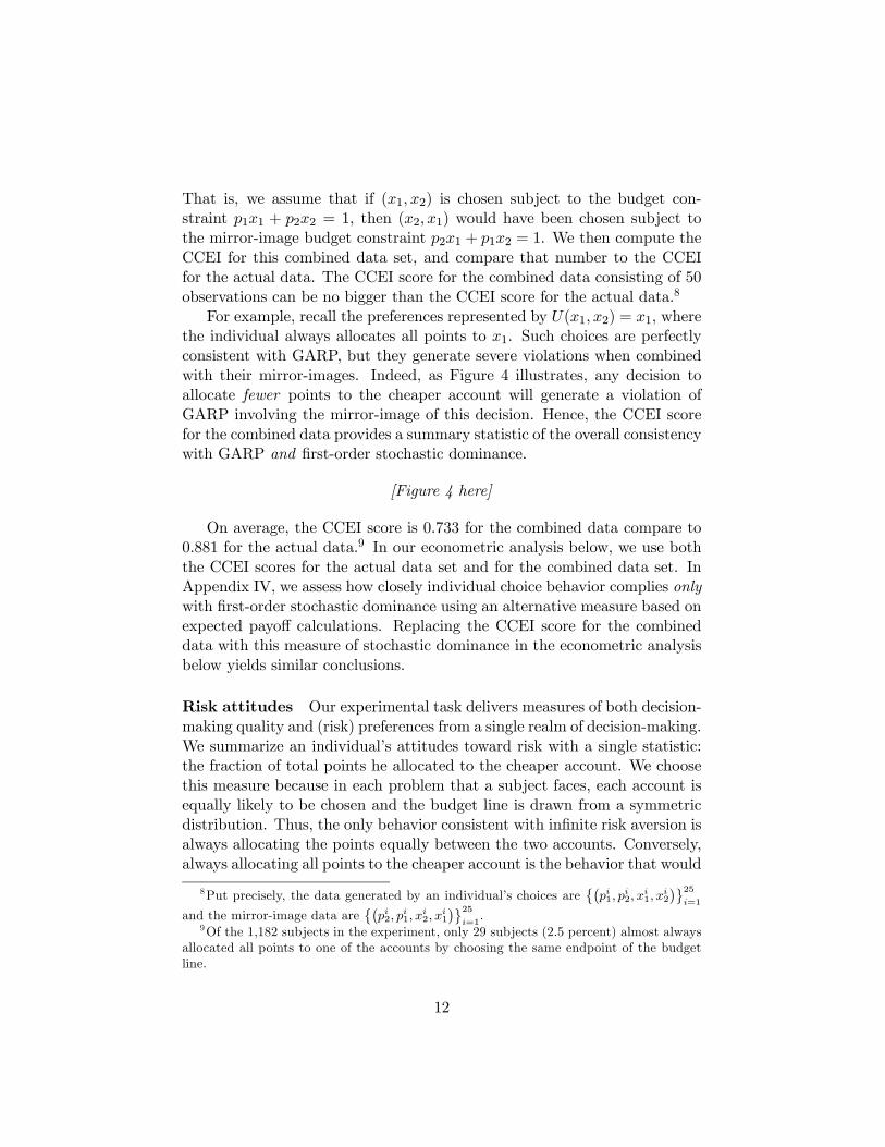
That is, we assume that if (1 2) is chosen subject to the budget con-

straint 11 + 22 = 1, then (2 1) would have been chosen subject to

the mirror-image budget constraint 21 + 12 = 1. We then compute the

CCEI for this combined data set, and compare that number to the CCEI

for the actual data. The CCEI score for the combined data consisting of 50

observations can be no bigger than the CCEI score for the actual data.8

For example, recall the preferences represented by (1 2) = 1, where

the individual always allocates all points to 1. Such choices are perfectly

consistent with GARP, but they generate severe violations when combined

with their mirror-images. Indeed, as Figure 4 illustrates, any decision to

allocate fewer points to the cheaper account will generate a violation of

GARP involving the mirror-image of this decision. Hence, the CCEI score

for the combined data provides a summary statistic of the overall consistency

with GARP and first-order stochastic dominance.

[Figure 4 here]

On average, the CCEI score is 0.733 for the combined data compare to

0.881 for the actual data.9 In our econometric analysis below, we use both

the CCEI scores for the actual data set and for the combined data set. In

Appendix IV, we assess how closely individual choice behavior complies only

with first-order stochastic dominance using an alternative measure based on

expected payoff calculations. Replacing the CCEI score for the combined

data with this measure of stochastic dominance in the econometric analysis

below yields similar conclusions.

Risk attitudes Our experimental task delivers measures of both decision-

making quality and (risk) preferences from a single realm of decision-making.

We summarize an individual’s attitudes toward risk with a single statistic:

the fraction of total points he allocated to the cheaper account. We choose

this measure because in each problem that a subject faces, each account is

equally likely to be chosen and the budget line is drawn from a symmetric

distribution. Thus, the only behavior consistent with infinite risk aversion is

always allocating the points equally between the two accounts. Conversely,

always allocating all points to the cheaper account is the behavior that would

8Put precisely, the data generated by an individual’s choices are1

2

1

2

25=1

and the mirror-image data are2

1

2

1

25=1.

9Of the 1,182 subjects in the experiment, only 29 subjects (2.5 percent) almost always

allocated all points to one of the accounts by choosing the same endpoint of the budget

line.

12

be implied by risk neutrality. More generally, subjects who are less averse

to risk will allocate a larger fraction of points to the cheaper account. Like

the revealed preference tests, an advantage of this measure is that it is non-

parametric. It measures attitudes toward risk without making assumptions

about the parametric form of the underlying utility function.10 Figure 5

displays the mean fraction of points allocated to the cheaper account and 95

percent confidence intervals across the socioeconomic categories. We note

that there is considerable heterogeneity in risk attitudes across categories,

which is characteristic of all these data, and that risk attitudes and CCEI

scores are effectively uncorrelated ( = 0113).11,12

[Figure 5 here]

4 Decision-making quality and socioeconomics

We next perform an analysis of the correlation between decision-making

quality — the consistency of the experimental data with GARP — and socioe-

conomic characteristics. Table 2 below presents the results of the economet-

ric analysis. In column (1), we present estimates with the CCEI scores for

the actual data set using ordinary least squares.13 The results show signif-

icant correlations. We obtain statistically significant coefficients in nearly

all socioeconomic categories, ranging in absolute values from about 0.025

to just over 0.050. Most notably, females, low-education, low-income, and

older subjects on average “waste” as much as 2.4, 2.6, 3.3, and 5.1 percentage

10 In parametric estimation, beyond the scope of this paper, we find that the choice data

of many subjects are well explained by a preference ordering in which the indifference

curves have a kink at the 45 degree line, corresponding to an allocation with a certain

payoff. One interpretation of this preference ordering is the disappointment aversion model

proposed by Gul (1991). This finding corroborates the results in Choi et al. (2007b) with

undergraduate students.11As Figure 5 shows, our individual-level measures of risk aversion are higher than the

measures reported in Choi et al. (2007b), but they are within the range of estimates from

recent studies (see Choi et al., 2007b, for a discussion of these studies).12The seminal paper by Holt and Laury (2002) also reports substantial low-stakes risk

aversion in the lab, as does Andersen et al. (2007) in the field. Risk aversion over moderate

stakes contradicts the validity of Expected Utility over wealth (Rabin, 2000, and Rabin

and Thaler, 2001). We emphasize that GARP does not imply the Savage (1954) axioms on

which Expected Utility is based and Expected Utility need not be assumed to investigate

the decision-making quality of choice under uncertainty.13To test for a potential misspecification, we used Ramsey’s (1969) RESET test by

adding the squared and cubed fitted values of the regression equation as additional re-

gressors, and found no evidence of misspecification (-value = 03098).

13

points more of their earnings, respectively, by making inconsistent choices.

In columns (2) we repeat the estimation reported in columns (1) using the

CCEI scores for the combined data set. The two scores are highly correlated

( = 0645) and, unsurprisingly, the results are qualitatively similar.

[Table 2 here]

The preceding analysis is based on the non-randomly selected subsample

of participants. The lack of observations on panel members who chose not to

participate or did not complete the experiment creates a missing data prob-

lem. We evaluate sample selection bias in our econometric analysis using

Heckman’s (1979) method. Our exclusion restriction involves the number of

completed CentERpanel questionnaires out of the total invitations to partic-

ipate in the three months prior to our experiment. This variable enters the

participation equation but, we assume, is conditionally uncorrelated with

the CCEI (see, Bellemare et al., 2008). To economize on space, the estima-

tion results are reported in Appendix V. The estimated parameters from the

OLS and the sample selection estimations are virtually identical. We inter-

pret these results to indicate that self-selection is not importantly driving

the results.

5 Wealth differentials and decision-making ability

The preceding analysis investigates the correlation between the consis-

tency scores and the sociodemographic characteristics of subjects. This

analysis makes no effort to evaluate a causal interpretation of these rela-

tionships. Nevertheless, the higher CCEI scores among high-income, high-

education, and younger subjects suggest that these groups may have better

economic outcomes, not only because they face fewer constraints or have

more normative preferences, but also because they tend to have superior

decision-making ability.

We next evaluate a causal interpretation of the correlation between the

CCEI scores and important economic outcomes in the real world. If hetero-

geneity in decision-making ability is an important source of heterogeneity

in economic outcomes, and if decision-making quality in the experiment as

measured by the CCEI is a good proxy for decision-making ability, then

differences in the CCEI scores across subjects should independently and

robustly explain differences in their real-world outcomes.

We focus on household wealth as the real-world economic outcome of

interest. As we argued, the investigation of wealth offers a strong test of

14

the idea that decision-making quality in the experiment captures decision-

making ability. Wealth is also of special interest because of a debate about

the sources of its dispersion. Bernheim et al. (2001) and Ameriks et

al. (2003) show substantial differences in wealth even among households

with very similar lifetime incomes, and provide evidence that differences

in decision-making ability drive wealth differentials. Scholz et al. (2006)

counter this by showing that, with detailed data on household-specific earn-

ings, a standard life-cycle model with homogeneous preferences can account

for more than 80 percent of the cross-sectional variation in wealth.

Our analysis of wealth proceeds in four steps. We first establish the

correlation between the CCEI and household wealth by estimating regres-

sions of the log of household wealth on socioeconomic variables (including a

flexible function of age), the log of household contemporaneous income, and

the consistency score of the person who is primarily responsible for house-

hold financial matters. Importantly, we follow a well-established tradition

in life-cycle analysis, and treat income, education, and family structure as

predetermined. We also evaluate the robustness of the conditional correla-

tion between the CCEI and wealth to changes in the functional form of the

estimating wealth equation.

Second, we demonstrate that this correlation is quantitatively robust to

the inclusion of additional controls for unobserved constraints, preferences,

and beliefs. If these unobservables were important sources of the observed

correlation, then adding the controls should have a substantial effect on the

estimated correlation between the CCEI and wealth. This analysis does not

seek the impossible goal of “controlling for everything” that might influence

wealth. Instead, in the spirit of Altonji et al. (2005), we examine whether

the conditional correlation we see between CCEI and wealth in the basic

specifications is much affected by the inclusion of additional controls that,

a priori, should be correlated with wealth through their correlation with

unobserved or misspecified variables.14

Third, we show that alternative measures of decision-making quality

(from the experiment) and decision-making ability (from the CentERpanel

survey) are not substitutes for the CCEI. The available alternatives either

14The reference to Altonji et al. (2005) underscores an analogy to the literature on

education. Economists have long struggled to identify and interpret the various effects

of education. The principal difficulty is that exogenous variation in education is rare

and limited in scope. But the topic is so important, that it justifies many approaches to

inference and interpretation. We view our paper in a similar vein; though, in the case of

decision-making quality, both the empirical and the theoretical literatures are much less

mature. Even the unconditional correlations presented above, were previously unknown.

15

have no independent power to predict wealth, or are not well-correlated with

consistency with GARP. Last, to account for the sources of the correlation

and to better understand which real-world decisions cause those with higher

CCEI scores to accumulate more wealth, we investigate the relationship

between the CCEI and the details of household saving allocations.

5.1 Establishing the correlation between CCEI and wealth

The CentERpanel collects information about wealth on an annual ba-

sis. Panel members are asked to identify a financial respondent who is “most

involved with the financial administration of the household.” All panel mem-

bers age 16 and older respond to questions about the assets and liabilities

that they hold alone. The financial respondent also provides information

about assets and liabilities that are jointly held by more than one household

member. The inventory covers checking and saving accounts, stocks, bonds

and other financial assets, real estate, business assets, mortgages, loans,

and lines of credit. Our analysis focuses on non-pension household wealth,

calculated by summing net worth over household members and taking the

household’s average over 2008 and 2009. The 703 households with wealth

data and a CCEI score from the household’s financial respondent had an

average household wealth of 164,130. Percentile values (in thousands ofEuros) are provided below.15

Min 1 5 10 25 50 75 90 95 Max

-180.7 -68.2 -4.8 0.0 10.8 93.0 242.1 523.8 955.6 3984.2

In our baseline specification, the sample size drops from 703 to 517 house-

holds (73.5 percent). This decline derives largely from three sources. First,

54 households (7.7 percent) have negative or missing household income in

2008, and 74 households (10.5 percent) have negative wealth and thus a

missing dependent variable. Second, younger households face incentives to

15The CentERpanel data do not include information on pension wealth. Nearly all

of the Dutch population is covered by the public pension system whose benefits are a

relatively simple function of family structure. A large majority of workers is also covered

by private pensions associated with their employment. Nearly all of these employment-

based plans are defined benefit, the vast majority of which pay benefits as a function of

earnings. Conditioning on family structure and earnings should, therefore, do much to

control for the incentives these pensions create for non-pension wealth accumulation. See

Alessie and Kapteyn (2001) and OECD (2009) for details about the pension systems in

the Netherlands. While it is a necessity, studying non-pension wealth has the advantage

of better isolating discretionary wealth accumulation.

16

hold less wealth as they borrow in order to invest or to smooth lifetime

consumption. With that in mind, we drop the 49 households (7.0 percent)

whose financial respondent is less than 35 years old. Finally, to reduce the

importance of extreme outliers, we drop the seven households that represent

the top and bottom half of one percent of the wealth distribution and the

bottom half of one percent of the CCEI distribution. Two additional house-

holds are dropped due to missing data on education. Our basic estimation

results are reported in Table 3 below.

Baseline In column (1), we present estimates from our baseline specifica-

tion using the sample of 517 households described above. The point estimate

of 1.35 for the coefficient on the CCEI indicates that a standard deviation

increase in the CCEI score of the household’s financial respondent is asso-

ciated with 18 percent more household wealth. As one might expect from

a relatively small sample of data on self-reported wealth, the standard er-

ror on this point estimate is fairly large. Nevertheless, we can reject a null

hypothesis of no relationship at the 5 percent level (p-value=0.017) with

standard errors robust to heteroskedasticity.16

Lifecycle In column (2), we repeat the estimation reported in column

(1) with the sample not restricted to households with financial respondents

who are at least 35 years old. Using the entire analysis sample, we find

that the point estimate on the CCEI is somewhat smaller, so a standard

deviation increase in the CCEI score of the household’s financial respondent

is associated with about 15 percent more household wealth. The standard

error on this point estimate implies that we can reject a null hypothesis of

no relationship with considerable confidence (p-value=0.038) but we cannot

reject a null hypothesis that the point estimates of the coefficient on the

CCEI reported in columns (1) and (2) are the same.

Levels The log specification in column (1) and (2) excludes households

with negative wealth, and may also cause small differences at positive but

very low levels of wealth to have large effects on point estimates. To eval-

uate the sensitivity of the results to the log specification, in column (3) we

estimate the regression in levels (of wealth and income) for the sample age

16The individual coefficients on age, education, and occuption are economically large,

but not statistically distinguishable from zero at standard levels of significance. A test of

their joint significance, however, rejects a null hypotheis of no relationship with a p-value

of 0.0002.

17

35 and older. We again see an economically large correlation between the

CCEI and levels of wealth, though this relationship is estimated somewhat

less precisely; the coefficient on the CCEI is significant only at the 10 percent

level (p-value=0.054).

[Table 3 here]

5.2 Evaluating a causal interpretation

We find an economically large and statistically significant correlation be-

tween the financial respondent’s CCEI score in the experiment and house-

hold wealth. This lends a basic level of support to the idea that our mea-

sure of decision-making quality from the experiment can proxy for decision-

making ability that applies across multiple real world choice domains. The

correlation between the CCEI and wealth may, however, not reflect decision-

making ability, but instead be due to a correlation between the CCEI and

other standard, but so far unobserved or misspecified, sources of heterogene-

ity in choice that affect wealth. To evaluate a causal relationship, we study

the robustness of the correlation with respect to the inclusion of additional

controls for unobserved constraints, preferences, and beliefs. Tables 4 and

5 present the estimates of the coefficients of interest. The full-length tables

are contained in Appendix VI.

Constraints We begin by investigating the correlation of the CCEI with

unobserved or misspecified constraints that affect the accumulation of wealth.

The estimation results are reported in Table 4 below. In standard lifecycle

models, wealth at a given age is a function of the constraints imposed by

the path of income over a lifetime. There is a variety of reasonable speci-

fications for a wealth regression, and our baseline specification reported in

Table 3 above is an especially simple benchmark. In column (1) of Table 4,

we assess the importance of the baseline linear-in-contemporaneous-income

specification by allowing income to enter in the form of a cubic. We see

virtually no change in the point estimate of the coefficient on the CCEI.

We thus find no evidence that the simple specification of contemporaneous

income drives the estimated relationship between the CCEI and wealth.

Another concern is that contemporaneous income is measured with er-

ror and the estimated coefficient on this variable is therefore biased toward

zero. The bias of this estimate then biases estimates of the coefficients on

other variables, including the CCEI. Standard lifecycle models predict con-

stant saving rates across lifetime income groups, and thus a unit elasticity

18

of wealth with respect to income (Dynan et al., 2004). If contemporaneous

income is a good proxy for lifetime income, then these theories predict the

coefficient on the log of contemporaneous income should equal one in the

baseline specification. In column (2), we impose this restriction and see

virtually no change in the point estimate of the coefficient on the CCEI.17

There is thus no evidence that measurement error in contemporaneous in-

come drives the main result.

A related concern is that contemporaneous income is a poor proxy for the

path of lifetime income, and unobserved aspects of that path are correlated

with the CCEI. We can evaluate this concern with some of the limited panel

data available on household income. To strike a balance between capturing

more income information and maintaining reasonable sample sizes, we go

back five years and use household income information for every other year.18

In column (3) of Table 4, we repeat the baseline specification reported in

column (1) of Table 3, this time restricting attention to the 449 households

(86.8 percent) for whom we have household income data from 2004 and

2006, as well as from 2008. In this smaller sample, the point estimate on

the CCEI remains economically large and statistically different from zero

(p-value=0.004). In column (4), we add controls for the log of household

income in 2004 and 2006. As a result, the magnitude of the coefficient on

the CCEI declines only slightly (by 0.037). We interpret this to indicate

that, while some of the correlation between the CCEI and wealth may be

attributable to a correlation between the CCEI and unobserved past income,

the available CentERpanel data on income provide little evidence that this

is the case.

An alternative approach is to take completed education as a proxy for

lifetime income. All of our specifications so far include indicators for each

level of education completed. It may be, however, that unobserved aspects

of education, such as the quality of schooling, are correlated with unob-

served elements of lifetime income which are, in turn, correlated with the

CCEI score in the experiment. If so, and if these unobserved constraints are

important sources of the observed correlation between CCEI and wealth,

then conditioning on completed education should have a substantial effect

17Brown (1976) shows that if theory makes a prediction about the coefficient on a

variable that is measured with error then restricting that coefficient to take on the value

predicted by theory will reduce the bias on the other coefficients being estimated.18The CentERpanel has been operating since 1993. However, income data for most

households who responded to the 2009 survey and completed our experiment do not go

back nearly that far. In cases where we have two out of the three income measures, we

use linear extrapolation to fill in the third.

19

on the estimated coefficient on the CCEI. In column (5) of Table 4, we repeat

the baseline specification reported in column (1) of Table 3 after omitting

the controls for the education of the financial respondent. Comparing the

estimates from these two specifications, we see that removing the educa-

tion controls increases the estimated coefficient on the CCEI only modestly

(by 0.090). In this way, we find little evidence that unobserved aspects of

education are driving the correlation between the CCEI and wealth.

[Table 4 here]

Preferences We have evaluated whether the correlation between the CCEI

and wealth is due to a relationship between the CCEI and unobserved or

misspecified income constraints. The results on education, which we took

to proxy for unobserved income but could also proxy for attitudes toward

risk and time, suggest that the relationship between the CCEI and unob-

served preferences is unlikely to play an important role. Nevertheless, we

next turn to analyze the possibility that the correlation between the CCEI

and wealth is driven by a relationship between the CCEI and unobserved

preferences that determine wealth. The estimation results are reported in

Table 5 below.

Our experimental task delivers individual-level measures of both decision-

making quality and risk preferences from a single realm of decision-making.

In column (1) of Table 5 we add to the baseline specification reported in

column (1) of Table 3 a control for risk attitudes by including a nonpara-

metric measure from the experiment discussed above — the average fraction

of points the financial respondent allocated to the cheaper account.19 The

point estimate on this quantitative measure indicates that risk tolerance in

the experiment is negatively associated with wealth. The coefficient is eco-

nomically large — a standard deviation increase in the fraction placed in

the cheaper account is associated with about seven percent less household

wealth — but imprecisely estimated. We cannot reject a null hypothesis of no

relationship (p-value=0.282) or a null of an economically large and positive

relationship. Given that risk attitudes and CCEI scores in the experiment

are effectively uncorrelated ( = 0113), it is unsurprising that the inclusion

of this control leaves the point estimate of the coefficient on the CCEI little

changed.

19To avoid the influence of extreme outliers, and to place this variable on more equal

footing with the CCEI, we also estimated a specification that omited the top and bot-

tom half of one percent of the distribution of this risk attitude measure, a total of six

households. The results are qualitatively similar.

20

It may be, however, that risk attitudes that influence wealth are not

well-correlated with risk preferences revealed over the small stakes of the

experiment. If so, qualitative measures of risk tolerance taken from the

CentERpanel survey instead of the experiment, may do better. In column

(2), we evaluate this possibility by also including a normalized measure of

risk-taking in investments.20 To preserve sample size, we also include a vari-

able to indicate whether the respondent provided a complete answer to these

questions. The results reinforce those from the previous specification. The

point estimate of the coefficient on the qualitative risk tolerance measure is

economically small, but imprecisely estimated. As important, the inclusion

of a qualitative measure of risk attitudes leaves the estimated coefficient on

the CCEI virtually unchanged. We thus find no evidence that these quali-

tative measures of risk attitudes from the survey are better able to capture

unobserved preferences, correlated with the CCEI, that influence wealth.

In a final effort to evaluate the importance of a correlation between

the CCEI and unobserved preferences, in column (3) we add to the list of

controls a conscientiousness measure from the “Big Five” test used for per-

sonality research in psychology.21 Again, to preserve sample size, we also

include a variable to indicate whether the respondent completed the consci-

entiousness questions. If not, we set their score to the sample mean (zero).

The magnitude of the coefficient on conscientiousness is large. A standard

20The CentERpanel survey contains six statements related to investment risk and return

such as “I think it is more important to have safe investments and guaranteed returns,

than to take a risk to have a chance to get the highest possible returns,” and “I want to be

certain my investments are safe.” Respondents are asked to evaluate the accuracy of these

statements as descriptions of themselves on a seven point scale. We sum the responses for

each respondent, when necessary re-ordering them so that higher scores reflect greater risk

tolerance. We then normalize the scores to have sample mean 0 and standard deviation

1.21The other Big Five personality traits are openness, extraversion, agreeableness, and

neuroticism. Among the Big Five, conscientiousness has the strongest correlation with

economic success (see, for examples, Barrick and Mount, 1991, and Tett et al., 1991).

Conscientious people are described as “thorough, careful, reliable, organized, industrious,

and self-controlled” (Duckworth et al., 2007). These terms suggest more patience, less

risk tolerance, and less taste for leisure. Conscientiousness may thus proxy for unobserved

preferences that influence wealth. The CentERpanel survey contains 10 statements related

to conscientiousness. The statements include: “I do chores right away,” “I am accurate

in my work,” among others. Respondents are asked to evaluate the accuracy of these

statements as descriptions of themselves on a five point scale. For each respondent, we

sum his or her responses to the 10 statements, and then normalize the scores to have

sample mean 0 and standard deviation 1. When necessary, we re-ordered the responses so

that higher scores reflect greater conscientiousness. Simultaneously adding other measures

from the Big Five yields the same conclusion. We omit those results for the sake of brevity.

21

deviation increase in conscientiousness is associated with about nine per-

cent more wealth. The standard error on the conscientiousness coefficient

is also relatively large, however, and we cannot reject a null hypothesis of

no correlation. Most important, adding the control for conscientiousness

has almost no effect on the coefficient on the CCEI. Thus we again find no

evidence that the relationship between the CCEI and wealth is driven by

a correlation between the CCEI and unobserved preferences that influence

wealth.

Beliefs Standard lifecycle models predict that beliefs, such as expectations

for longevity, income, or asset returns, should affect household wealth levels.

The CentERpanel collects relatively little information about respondents’

beliefs, but the survey does ask questions about expected longevity. We

can therefore use these data to evaluate the extent to which the correlation

between the CCEI and wealth accumulation is attributable to a correlation

between the CCEI and some unobserved beliefs that influence wealth. To

strike a balance between capturing more information and maintaining the

sample sizes, we consider a measure of longevity expectations based on the

question answered by the largest number of respondents.22

In column (4) of Table 5, we repeat the baseline specification reported in

column (1) of Table 3, this time restricting attention to the 414 households

(80.0 percent) for whom the financial respondent answered this question

about longevity. In this smaller sample, the point estimate of the coefficient

on the CCEI remains economically large, though a larger standard error

reduces the statistical significance (p-value=0.053). In column (5), we add

the control for longevity expectations. This measure, itself, has little power

to predict wealth levels and including it increases the estimate of the coef-

ficient on the CCEI very slightly (by 0.023). Thus, while we have limited

ability to explore this issue with available data, we find no evidence that a

relationship between the CCEI and unobserved beliefs drives the correlation

between the CCEI and wealth.

[Table 5 here]

22The question answered by the largest number of respondents asks “How likely is it

that you will attain (at least) the age of 80?” Responses are recorded on a scale from 0

to 10, and respondents are instructed to interpret 0 to mean “no chance at all” and 10 to

mean “absolutely certain.”

22

5.3 Evaluating alternatives to the CCEI

We have found an economically large, statistically significant, and quan-

titatively robust relationship between the CCEI scores in the experiment and

wealth. We next evaluate whether alternative laboratory- and survey-based

measures can substitute for the CCEI for the purposes of explaining wealth.

Measuring decision-making quality by consistency with GARP has strong

theoretical and methodological justifications, but augmenting GARP with

additional, normative criteria might better capture decision-making quality.

It is also possible that, while lacking in theoretical foundations, other proxies

for decision-making ability are so well-correlated with the CCEI that they

may serve as substitutes for the CCEI. This would be especially useful if the

other proxies are readily available on surveys or in administrative datasets.

The estimation results are reported in Table 6 below. The full-length table

is contained in Appendix VI.

Stochastic dominance We begin with consideration of a stronger notion

of decision-making quality derived from our experiment. In column (1)

of Table 6 we repeat the estimation of the baseline specification reported

in column (1) of Table 3 after adding the CCEI scores for the combined

data set (combining the actual data from the experiment and the mirror-

image data). As explained above, this test of decision-making quality is

stronger because it demands both consistency with GARP and first-order

stochastic dominance. We find no evidence that, conditional on the CCEI

score from the actual data, the CCEI score for the combined data set has an

independent relationship with wealth. Adding the CCEI for the combined

data set as a regressor has only a modest effect on the point estimate of the

coefficient on the CCEI, though the standard error on this estimate increases.

The point estimate of the coefficient on the CCEI for the combined data set

is small, but imprecisely estimated. These results are consistent with the

idea that the CCEI for the combined data set, while requiring a compelling

and generally accepted notion of decision-making quality, merely represents

a noisier measure of the aspects of decision-making ability captured by the

CCEI scores for the actual data set.

Trembling von Gaudecker et al. (2011) conducted risk experiments with

CentERpanel members using a multiple price list design (Andersen et al.,

2006). They estimated a flexible parametric model that includes an indi-

vidual “trembling” parameter measuring “the propensity to choose ran-

domly rather than on the basis of preferences.” von Gaudecker et al. (2011)

23

conclude that “while many people exhibit consistent choice patterns, some

have very high error propensities.” That parameter can be interpreted as

a measure of decision-making quality as it captures the degree to which

an individual’s choices are consistent both with rationality and with some

assumptions about the functional form of utility. This contrasts with the

CCEI, which makes no assumptions about the structure of preferences. The

CCEI and the “trembling” parameter of von Gaudecker et al. (2011) are

only moderately correlated ( = 0178) in the overlapping sample of 624

subjects (43.9 percent) who participated in both experiments. As a result,

we can gain some insight into the relationship between wealth and consis-

tency with the utility-maximizing model versus consistency with a class of

utility functions commonly employed in the empirical studies.

In column (2) of Table 6, we repeat the estimation of the baseline speci-

fication reported in column (1) of Table 3, this time restricting attention to

the 326 households (63.1 percent) with a financial respondent who partici-

pated in both experiments.23 In column (3) we add to the list of regressors a

variable equal to (1−) in von Gaudecker et al. (2011). The point estimateof the coefficient on this parameter is large — a standard deviation increase

is associated with 17 percent more household wealth — and we can reject

a null hypothesis of no relationship at the 10 percent confidence level (p-

value=0.057). The estimated coefficient on the CCEI is reduced somewhat

when we include this estimate, but remains economically large and statisti-

cally significant at the 10 percent confidence level (p-value=0.083). There

are many possible reasons for the differences in these two measures and their

relationship to wealth — they are based on different methods, derived from

different designs, and elicited in different experiments. Intriguingly, however,

the results suggest substantial differences between decision-making quality

measured by the restrictions imposed by the utility-maximization model and

additional restrictions imposed by various hypotheses concerning functional

structure. This is an interesting avenue for future work with more data on

both measures.

Cognitive ability Tests of cognitive ability (IQ) might also capture as-

pects of decision-making ability (cf. Dohmen, et al., 2010.) Different from

IQ tests, consistency with GARP offers a theoretically disciplined measure

for decision-making quality that has a well-established economic interpre-

23To place the two measures on more equal footing, we trim the lowest one half of

one percent of the distribution of each of the measures (two obervations each) in the

overlapping sample.

24

tation. There is no comparable, theoretically disciplined, means of using

and interpreting an IQ test. Nevertheless, if the CCEI and IQ were very

well-correlated, then analysts interested in measuring decision-making abil-

ity might be able to replace the revealed preference tests with one of the

many IQ tests and, in some circumstances, the conceptual distinctions be-

tween the measures would have little practical import. It seems likely that

the capacity to make choices of high decision-making quality draws on skills

of analysis and perception that also improve IQ test scores. But if the goal

is to isolate the influence of these skills on decision-making ability, rather

than on constraints, information, or beliefs, are the CCEI and IQ scores

substitutes?

Many IQ tests are precluded from wide use by intellectual property rights

or are impossible to implement in Internet panels. The CentERpanel has

not implemented any of the well-known and wide-ranging IQ instruments.

However, in connection with our and other researchers’ projects, the Cen-

tERpanel asked a sample of respondents to complete Frederick’s (2005) Cog-

nitive Reflection Test and a brief Raven’s Progressive Matrices Test.24 We

omit the Raven’s test because it generated effectively no variation in re-

sponses. Among the 467 subjects who completed the Cognitive Reflection

Test and participated in our experiment, the correlation between the CCEI

and the Cognitive Reflection Test is positive, but the variables are far from

collinear ( = 0193). This result echoes Burks et al. (2009) who find a corre-

lation of approximately 0.22 between IQ and compliance with monotonicity

(measured by more than one switch point in multiple price list experiments

regarding risk and time tradeoffs). To assess the predictive content of the

CCEI and the Cognitive Reflection Test, in column (4) in Table 6 we add the

number of questions answered correctly in the Cognitive Reflection Test to

the baseline specification. To preserve sample size, we also include a variable

to indicate whether a Cognitive Reflection Test score was available for the

household’s financial respondent. For those who had no score, we substitute

the mean of the distribution of the rest of the sample.

The point estimate of the coefficient on the Cognitive Reflection Test

is economically large — answering one more of the three questions on the

24The Cognitive Reflection Test consists of three questions. Each question is designed

to have an intuitive, but incorrect, answer. The intuitive answer tends to spring to mind

and then require reflection in order to dismiss. One question asks “A bat and a ball cost

$1.10 in total. The bat costs $1.00 more than the ball. How much does the ball cost?”

Here the intuitive answer is $0.10, but the correct answer is $0.05. Frederick (2005) shows

that this test is well correlated with a 50-question test of general cognitive ability, as well

as tests of achievement such as the Scholastic Achievement Test (SAT).

25

Cognitive Reflection Test correctly is associated with about 12 percent more

wealth — and statistically significant at the 10 percent level (p-value=0.094).

Adding this measure, and the missing indicator, to the basic specification

reduces the estimated coefficient on the CCEI somewhat, but about a fifth of

the reduction is due to the inclusion of the indicator for a missing Cognitive

Reflection Test score. These results suggest that the Cognitive Reflection

Test captures some decision-making ability related both to decision-making

quality in the experiment and wealth accumulation. The findings also in-

dicate, however, that this measure of cognitive ability cannot be used as a

simple substitute for the CCEI for the purposes of explaining wealth.25

[Table 6 here]

5.4 The sources of correlation between CCEI and wealth

We found an economically large and statistically significant correlation

between household wealth and the financial respondent’s CCEI score in the

experiment. We saw that this correlation is robust to the inclusion of con-

trols for unobserved preferences, constraints, and beliefs, and that alterna-

tive measures of decision-making quality or decision-making ability elicited

in an experiment or a survey are not substitutes for the CCEI. With these

results in mind, we now turn to account for the sources of the correlation by

investigating the relationship between the CCEI and the details of house-

hold saving allocations. Our goal is to better understand which important

real-world decisions cause those who appear to have better decision-making

ability to accumulate more wealth. These estimation results are reported in

Table 7. The full-length table is contained in Appendix VI.

Portfolio In columns (1)-(6) of Table 7, we present estimates that re-

late the CCEI score of the household’s financial respondent to whether the

household has a checking account, a savings account, owns stocks, and the

fraction of the household’s wealth held in each of these assets. To reduce

the importance of extreme outliers, in all specification we drop households

whose fraction of wealth in the relevant category (checking, saving, stocks,

housing) is less than -0.15 or greater than 1.15. The results provide some

25Perhaps related to Cognitive Reflection Test and the tendency to reflect upon choices,

adding a control for subjects’ response times in the experiment has virtually no effect on

the coefficient on the CCEI. This is expected given the modest unconditional correlation

between the CCEI scores and response times ( = −0075). We also cannot reject a nullhypothesis of no correlation between the response time and wealth. These results are

omitted in the interest of brevity.

26

evidence that, conditional on household characteristics, contemporaneous in-

come, occupation and education level, households with financial respondents

with higher CCEI scores put less of their wealth in low-risk and low-return

assets such as checking and savings accounts. The coefficients on the CCEI

in columns (2) and (4) are modest in magnitude but statistically significant

at the 10 percent level (p-values of 0.083 and 0.095, respectively). The re-

sults also provide some evidence that individuals with higher CCEI scores

are somewhat more likely to participate in the stock market, though this

relationship is not statistically distinguishable from zero.

Housing Finally, the coefficients on the CCEI in columns (7) and (8)

show economically substantial and statistically significant correlations be-

tween the CCEI and decisions regarding home ownership. Households with

financial respondents with higher CCEI scores are more likely to own a

home and they put a larger fraction of their household’s wealth in a home.

A standard deviation increase in the CCEI of the financial respondent is

associated with an increase of 0.047 in the probability of owning a home.

Similarly, a standard deviation increase in the CCEI is associated with an

increase of 0.043 in the fraction of wealth held in housing. The tendency

for those with higher CCEI scores to own a home and put more of their

wealth in housing is especially interesting given the favorable tax treatment

of owner-occupied housing in the Netherlands, which gives home ownership

an important advantage over renting and, other things equal, means wealth

placed in mortgaged housing pays a substantial premium.26 So long as hous-

ing supply is somewhat elastic, and thus the incidence of these tax benefits

are shared between buyers and sellers, this suggests that owning a home and

placing more wealth in mortgaged housing are often high decision-making

quality financial choices. If so, the positive correlation between the CCEI

and these decisions is what we would expect if the CCEI captured a general

tendency toward higher (financial) decision-making ability.

26About 69 percent of households in the sample own a home, and the average fraction

of wealth held in housing is approximately 54 percent. In the Netherlands, assets held

in owner-occupied housing are not subject to the usual capital income tax. If they were,

four percent of housing value would be treated as implicit income and taxed at 30 percent.

Instead, imputed rent is presumed to be very low (0.55 percent of housing value), is subject

to the progressive tax on labor income, and that tax is not due unless the household claims

a deduction for mortgage interest. Nominal mortgage interest is, in turn, fully deductable

from taxable income. Thus, for purposes of federal taxation, housing assets underwritten

by a mortgage will typically pay a negative rate of return. In this way, according to van

Ewijk et al. (2007), the Netherlands offers by far the most favorable tax treatment of

owner occupied housing in Western Europe.

27

[Table 7 here]

6 Related literature

This paper is primarily concerned with a relatively new economics liter-

ature that emphasizes a gap between what people actually choose and what

they would have chosen if they were fully attentive to their choices and had

the skills and knowledge necessary to weigh costs and benefits in often com-

plex settings. This research provides evidence that some choices are better

than others and some individuals are better decision-makers than others.

This new literature contrasts standard economic analysis which takes a

libertarian approach; in the absence of the complete data required, stan-

dard analysis assumes that all choices are of good decision-making quality

and that everyone has sufficient decision-making ability. The libertarian ap-

proach has obvious appeal, and economists in the new literature have strug-

gled to measure decision-making quality and to separately identify decision-

making ability from standard sources of heterogeneity in important economic

outcomes. That is, the new studies have been subject to identification and

measurement problems and confronted them to different degrees.

Observational studies of market data have shown that some individuals

make choices of such poor decision-making quality that they clearly leave

“money on the table.” Agarwal et al. (2009) is a prominent example. That

paper provides evidence of strictly dominated choices regarding the use of

credit. Importantly, research like this requires an uncommonly high-quality

(administrative) dataset that makes the relevant tradeoffs very clear. The

comprehensive nature of the data makes classifying some decisions as “mis-

takes” immediate and indisputable, and thus allows the analyst to avoid both

the measurement and the identification problem. However, such administra-

tive datasets provide information about the activity at just one retailer, or

on just a few credit cards, or in just one form of saving. They thus capture

only a slice of the economic activities of the individuals involved.27 As a

result, they cannot reveal whether a lower decision-making quality choice

represents a minor bobble in otherwise sound decision-making, or a more

fundamental problem in evaluating economic choices due to lack of decision-

making ability.

27Other examples of strictly observational studies of decision-making quality that focus

on “slices” of economic activity include Miravete (2003) on cell phone calling plans, Choi

et al. (2011) on employer-sponsored saving, Ketcham et al. (2012) on health insurance,

and Lacetera et al. (2012) on car purchases.

28

Experiment- or survey-based studies take a different approach. They

confront the identification problem using measures of education, cognitive

and non-cognitive skills, or financial literacy as proxies for decision-making

ability and either instrumental variables or experimental manipulation to

infer causal effects. A prominent example of this research is Ameriks et al.

(2003). That paper provides evidence that differences in individuals’ plan-

ning abilities, rather than more standard sources of heterogeneity, explain

important variation in wealth. Other examples of significant research in

this vein include Bernheim and Garret (2003) and Duflo and Saez (2003)

who study the effect of employer-based financial education on saving. Re-

search of this kind relaxes the imposing data requirements of observational

studies that investigate decision-making quality directly, but it is silent on

the measurement problem. It does not seek a portable, quantitative, and

economically interpretable measure of decision-making quality.

Other related research relies importantly on surveys and is more strictly

descriptive. Restricting attention just to financial decision-making, this re-

search includes Lusardi and Mitchell (2007) who document very low levels of

financial planning, financial literacy, and a positive correlation between lit-

eracy, financial planning and wealth; and Fang et al. (2008), who find that,

rather than measures of risk preferences, cognitive functioning stands out as

a significant predictor of Medigap purchase. Agarwal and Mazumder (2013)

correlate proxies of decision-making ability, namely mathematical and non-

mathematical cognitive tests, with making low quality financial decisions

involving the use of credit.28

Our approach follows the strictly observational studies by defining decision-

making quality and measuring it directly. Different from that literature, we

define decision-making quality by the consistency of choices with GARP, and

we measure it by the extent of GARP violation using the CCEI and other

standard indices that have been proposed for this purpose. Like the exper-

imental literature, we seek to isolate decision-making ability from standard

sources of heterogeneity in choice, in our case by presenting individuals with

a theoretically-grounded economic choice experiment designed to provide a

28Special attention has been paid in this literature to older populations, reflecting a

concern about decreasing decison-making ability later in life. The papers in the Novem-

ber 2010 issue of the Economic Journal (Volume 120, Issue 548) offer nice reviews: Banks

(2010) summarizes research on the relationships between cognitive function, financial lit-

eracy and financial outcomes at older ages; Smith et al. (2010) and Banks et al. (2010)

show that wealth and retirement saving patterns are associated with numerical and other

cognitive abilities at middle and older ages; and Van Den Berg et al. (2010) and Jappelli

(2010) explore causes of the differences in cognitive function and financial literacy in later

life.

29

stringent test of consistency with GARP.

Echenique et al. (2011) measure consistency with revealed preference

conditions in individual-level data on grocery store expenditures, and cor-

relate the degree of consistency with some indicators of family size, income,

age, and education. Their measure is based on the idea that an individual

who violates GARP can be exploited as a “money pump.” We refer the

interested reader to Appendix II for the construction of the money pump

index. To our knowledge, no other papers analyze the correlation between

consistency with GARP and socioeconomic characteristics in a broad pop-

ulation. Echenique et al. (2011) conclude that “the hypothesis of consumer

rationality cannot be rejected.” Such consumption data can, however, lack

power to reject violations of GARP (Blundell et al., 2003, 2008). The power

of the test depends on the range of prices consumers face (the frequency

with which budget lines cross) and the number of choices each consumer

makes.

7 Concluding remarks

We offered a new large-scale experiment — employing graphical repre-

sentations of standard consumer decision problems and using a diverse pool

of subjects — that enables us to collect richer data than has been possible

in the past. These data allow us to say that some sets of choices are of

better decision-making quality than others, in that some choices are more

rational than others. Because the data are provided by a large and het-

erogenous sample, we can analyze the correlates of decision-making quality

in the laboratory and relate it to important economic outcomes like wealth.

We find that differences in the experimental measures of decision-making

quality across subjects independently and robustly explain differential pat-

terns of wealth across households. Since wealth accumulation is determined

by countless decisions, made over time in many environments, and involv-

ing a host of different tradeoffs, our findings indicate that our measure of

decision-making quality captures aspects of decision-making ability that ap-

ply across many sorts of economic choice problems. This study therefore

suggests a new path toward solving the twin problems of identification and

measurement.

We conclude by underscoring three key features of the approach we have

taken here. First, our measure of decision-making quality — the consistency

of choices with GARP — dictates the experimental task: a canonical problem

of selecting an allocation from a budget line. Given the task, the measure

30

also provides the benchmark level of consistency necessary to provide a rig-

orous test. There are no comparable, theoretically disciplined, means of

quantifying, interpreting, and evaluating laboratory or survey measures of

decision-making ability, namely tests of cognitive and non-cognitive skills.

Second, informed by economic theory, the single experimental task deliv-

ers measures of both decision-making quality and preferences from a unified

realm of decision-making. Relevant preferences cannot be recovered from

performance on standard psychological tests. Third, unlike many tests of

cognitive abilities or personality traits, revealed preference tests are applica-

ble to, and comparable across, all sorts of economic choice problems. Our

approach can thus be transported, with relative ease, to different decision

domains. We can make domain-specific predictions and provide a unified

measure of decision-making quality across domains. In all of these ways, the

theoretical foundation of our approach drives the design of the experiment

and allows diverse and disciplined use of the resulting data.

Taken together, our findings provide new evidence on three important

issues: () the validity of measuring decision-making quality by the consis-

tency of choices with economic rationality, () the feasibility of testing for

consistency with rationality through a web-based survey on a large scale,

() the relative importance of heterogeneity in decision-making ability for

understanding important economic outcomes. This last issue commands

special attention because decision-making ability, unlike preferences, may

be justifiably manipulated. If differences in decision-making ability are im-

portant sources of the heterogeneity in economic outcomes, then even quite

costly policy changes aimed at “soft” or “libertarian” paternalism may hold

substantial promise.29

References

[1] Afriat, S. (1967) “The Construction of a Utility Function from Expen-

diture Data.” Econometrica, 6, pp. 67-77.

[2] Afriat, S. (1972) “Efficiency Estimates of Production Functions.” In-

ternational Economic Review, 8, pp. 568-598.

29The prominent forms of light or soft paternalism are libertarian paternalism (Thaler

and Sunstein, 2003) and asymmetric paternalism (Camerer et al., 2003). Loewenstein and

Haisley (2008) and Kariv and Silverman (2013) provide relevant discussions.

31

[3] Agarwal, S., J. Driscoll, X. Gabaix and D. Laibson (2009) “The Age of

Reason: Financial Decisions over the Life-Cycle with Implications for

Regulation.” Brookings Papers on Economic Activity, 2, pp. 51-117.

[4] Agarwal, S. and B. Mazumder (2013) “Cognitive Abilities and House-

hold Financial Decision Making.”American Economic Journal: Applied

Economics, 5, pp. 193-207.

[5] Alessie, R. and A. Kapteyn (2001) “Savings and Pensions in The

Netherlands.” Research in Economics, 55, pp. 61-82.

[6] Altonji, J., T. Elder and C. Taber (2005) “Selection on Observed and

Unobserved Variables: Assessing the Effectiveness of Catholic Schools.”

Journal of Political Economy, 113, pp. 151-184.

[7] Ameriks, J., A. Caplin and J. Leahy (2003) “Wealth Accumulation

and the Propensity to Plan.” Quarterly Journal of Economics, 118, pp.

1007-1047.

[8] Andersen, S., G. Harrison, M. Lau and E. Rutström (2006) “Elicitation

Using Multiple Price List Formats.” Experimental Economics, 9, pp.

383-405.

[9] Andersen, S., G. Harrison, M. Lau and E. Rutström (2007) “Estimat-

ing Risk Attitudes in Denmark: A Field Experiment.” Scandinavian

Journal of Economics 109, pp. 341-368.

[10] Banks, J. (2010) “Cognitive Function, Financial Literacy and Financial

Outcomes at Older Ages: Introduction.” Economic Journal, 120, pp.

357-362.

[11] Banks, J., C. O ’Dea and Z. Oldfield (2010) “Cognitive Function, Nu-

meracy and Retirement Saving Trajectories.” Economic Journal, 120,

pp. 381-410.

[12] Barrick, M. and M. Mount (1991) “The Big Five Personality Dimen-

sions and Job Performance: A Meta-analysis.” Personnel Psychology,

44, pp. 1-26.

[13] Bellemare, C., S. Kröger and A. van Soest (2008) “Measuring Inequity

Aversion in a Heterogeneous Population Using Experimental Decisions

and Subjective Probabilities.” Econometrica, 76, pp. 815-839.

32

[14] Bernheim, D. and D. Garrett (2003) “The Effects of Financial Educa-

tion in the Workplace: Evidence from a Survey of Households.” Journal

of Public Economics, 87, pp. 1487-1519.

[15] Bernheim, D. and A. Rangel (2009) “Beyond Revealed Preference:

Choice-Theoretic Foundations for Behavioral Welfare Economics.”

Quarterly Journal of Economics, 124, pp. 51-104.

[16] Bernheim, D., J. Skinner and S. Weinberg (2001) “What Accounts for

the Variation in Retirement Wealth among U.S. Households?” Ameri-

can Economic Review, 91, pp. 832-857.

[17] Blundell R., M. Browning and I. Crawford (2003) “Nonparametric En-

gel Curves and Revealed Preference.” Econometrica, 71, pp. 205-240.

[18] Blundell R., M. Browning and I. Crawford (2008) “Best Nonparametric

Bounds on Demand Responses.” Econometrica, 76, pp. 1227-1262.

[19] Brown, C. (1976) “A Model of Optimal Human-Capital Accumulation

and the Wages of Young High School Graduates.” Journal of Political

Economy, 84, pp. 299-316.

[20] Burks, S., J. Carpenter, L. Goette, and A. Rustichini (2009) “Cogni-

tive Skills Affect Economic Preferences, Strategic Behavior, and Job

Attachment.” Proceedings of the National Academy of Sciences, 106,

pp. 7745-7750.

[21] Camerer, C., S. Issacharoff, G. Loewenstein, T. O’Donoghue and M.

Rabin (2003) “Regulation for Conservatives: Behavioral Economics and

the Case for Asymmetric Paternalism.” University of Pennsylvania Law

Review, 151, pp. 1211-1254.

[22] Choi, J., D. Laibson and B.Madrian (2011) “$100 Bills on the Side-

walk: Suboptimal Investment in 401(k) Plans.” Review of Economics

and Statistics, 93, pp. 748-763.

[23] Choi S., R. Fisman, D. Gale, and S. Kariv (2007a) “Revealing Prefer-

ences Graphically: An Old Method Gets a New Tool Kit.” American

Economic Review, Papers & Proceedings, 97, pp. 153-158.

[24] Choi S., R. Fisman, D. Gale, and S. Kariv (2007b) “Consistency and

Heterogeneity of Individual Behavior under Uncertainty.” American

Economic Review, 97, pp. 1921-1938.

33

[25] Dohmen, T., A. Falk, D. Huffman and U. Sunde (2010) “Are Risk Aver-

sion and Impatience Related to Cognitive Ability?”American Economic

Review, 100, pp. 1238-1260.

[26] Duflo, E. and E. Saez (2003) “The Role of Information and Social In-

teractions in Retirement Plan Decisions: Evidence From a Randomized

Experiment.” Quarterly Journal of Economics, 118, pp. 815-842.

[27] Dynan, K., J. Skinner and S. Zeldes (2004) “Do the Rich Save More?”

Journal of Political Economy, 112, pp. 397-444.

[28] Duckworth A., C. Peterson, M. Matthews and D, Kelly (2007) “Grit:

Perseverance and Passion for Long-term Goals.” Journal of Personality

and Social Psychology, 92, pp. 1087-1101.

[29] Echenique, F., S. Lee and M. Shum (2011) “The Money Pump as a Mea-

sure of Revealed Preference Violations.” Journal of Political Economy

119, pp. 1201-1223.

[30] Fang, H., M. Keane and D. Silverman (2008) “Sources of Advantageous

Selection: Evidence from the Medigap Insurance Market.” Journal of

Political Economy, 116, pp. 303-350.

[31] Fisman, R., S. Kariv and D. Markovits (2007) “Individual Preferences

for Giving.” American Economic Review, 97, pp. 1858-1876.

[32] Frederick, S. (2005) “Cognitive Reflection and Decision Making.”

Journal of Economic Perspectives, 19, pp. 25-42.

[33] Gul, F. (1991) “A Theory of Disappointment in Decision Making under

Uncertainty.” Econometrica, 59, pp. 667—686.

[34] Heckman, J. (1979) “Sample Selection Bias as a Specification Error.”

Econometrica, 47, pp. 153-161.

[35] Holt, C. and S. Laury (2002) “Risk Aversion and Incentive Effects.”

American Economic Review, 92, pp. 1644-1655.

[36] Jappelli, T. (2010) “Economic Literacy: An International Comparison.”

Economic Journal, 120, pp. 429-451.

[37] Kahneman, D. and A. Tversky (1984) “Choices, values and frames.”

American Psychologist, 39, pp. 341—350.

34

[38] Kariv, S. and D. Silverman (2013) “An Old Measure of Decision-making

Quality Sheds New Light on Paternalism.” Journal of Institutional and

Theoretical Economics, 169, pp. 29-44.

[39] Ketcham, J., C. Lucarelli, E. Miravete and C. Roebuck (2012) “Sink-

ing, Swimming, or Learning to Swim in Medicare Part D.” American

Economic Review, 102, pp. 2639-2673.

[40] Koszegi, B. and M. Rabin (2006) “A Model of Reference-Dependent

Preferences.” Quarterly Journal of Economics, 121, pp. 1133-1165.

[41] Lacetera, N., D. Pope and J. Sydnor (2012) “Heuristic Thinking and

LimitedAttention in the Car Market.”American Economic Review, 102,

pp. 2206-2236.

[42] Loewenstein, G. and E. Haisley (2008) “The Economist as Therapist:

Methodological Ramifications of “Light” Paternalism.” In The Foun-

dations of Positive and Normative Economics, ed. A. Caplin and A.

Schotter. Oxford University Press.

[43] Lusardi, A. and O. Mitchell (2007) “Baby Boomer Retirement Secu-

rity: The Roles of Planning, Financial Literacy, and Housing Wealth.”

Journal of Monetary Economics, 54, pp. 205-224.

[44] Miravete, E. (2003) “Choosing the Wrong Calling Plan? Ignorance and

Learning.” American Economic Review, 93, pp. 297-310.

[45] OECD (2009) “Pensions at a Glance 2009: Retirement-Income Systems

in OECD Countries.” URL: www.oecd.org/els/social/pensions/PAG.

[46] Quiggin, J. (1990) “Stochastic Dominance in Regret Theory.” Review

of Economic Studies, 57, pp. 503-511.

[47] Rabin, M. (2000) “Risk Aversion and Expected-utility Theory: A Cal-

ibration Theorem.” Econometrica, 68, pp. 1281-1292.

[48] Rabin, M. and R. Thaler (2001) “Anomalies: Risk Aversion.” The Jour-

nal of Economic Perspectives, 15, pp. 219-232.

[49] Ramsey, J. (1969) “Tests for Specification Errors in Classical Linear

Least-squares Regression Analysis.” Journal of the Royal Statistical So-

ciety, 31, pp. 350-371.

[50] Samuelson, P. (1947) Foundations of Economic Analysis. Cambridge:

Harvard University Press.

35

[51] Savage, L. J. (1954) The Foundations of Statistics. New York: Wiley.

[52] Scholz, J., A. Seshadri and S. Khitatrakun (2006) “Are Americans Sav-

ing “Optimally” for Retirement?” Journal of Political Economy, 114,

pp. 607-643.

[53] Smith, J., J. McArdle and R. Willis (2010) “Financial Decision Making

and Cognition in a Family Context.” Economic Journal, 120, pp. 363-

380.

[54] Tett, P., D. Jackson, and M. Rothstein (1991) “Personality Measures as

Predictors of Job Performance: A Meta-Analytic Review.” Personnel

Psychology, 44, pp. 703-742.

[55] Thaler, R. and C. Sunstein (2003) “Libertarian Paternalism.” American

Economic Review, Papers & Proceedings, 93, pp. 175-179.

[56] van Den Berg, G., D. Deeg, M. Lindeboom and F. Portrait (2010) “The

Role of Early-Life Conditions in the Cognitive Decline due to Adverse

Events Later in Life.” Economic Journal, 120, pp. 411-428.

[57] van Ewijk, C., B. Jacobs and R. de Mooij (2007) “Welfare Effects of Fis-

cal Subsidies on Home Ownership in the Netherlands.” De Economist,

155, pp. 323-336.

[58] von Gaudecker, H-M., A. van Soest and E. Wengström (2011) “Hetero-

geneity in Risky Choice Behaviour in a Broad Population.” American

Economic Review, 101, pp. 1-33.

[59] Wakker, P. (1993) “Savage’s Axioms Usually Imply Violation of Strict

Stochastic Dominance.” Review of Economic

36

Participants DropoutsNon-

participantsFemale 45.43 37.89 50.00Age

16-34 18.53 3.16 26.1435-49 26.14 12.11 32.1350-64 35.62 38.42 27.5865+ 19.71 46.32 14.15

EducationLow 33.59 42.63 30.99Medium 29.70 22.63 31.61High 36.72 34.74 37.40

Household monthly income€0-2500 22.42 34.73 21.28€2500-3499 25.13 26.32 18.90€3500-4999 28.85 16.32 28.93€5000+ 23.60 22.63 30.89

Occupation

Table 1. Sociodemographic information

OccupationPaid work 53.13 39.47 62.91House work 11.59 7.89 8.78Retired 20.90 42.63 13.95Others 14.38 10.00 14.36

Household compositionPartner 80.88 67.89 82.64# of children 0.84 0.32 1.09

# of obs. 1182 190 968Participants completed the experiment, dropouts logged in and quit the experiment, and nonparticipants wererecruited for the experiment but never logged in. The low, medium and high education levels correspond toprimary or pre-vocational secondary education, pre-university secondary education or senior vocational training,and vocational college or university education, respectively. We use household monthly gross income-levelcategories such that the proportions of participants in each category are approximately equal. The classification oflevels of completed education and occupations arebased on the categorization of Statistics Netherlands (CentraalBureau voor de Statistiek).

(1) (2)0.887*** 0.735***(0.022) (0.037)

0 024*** 0 011

Table 2. The correlation between CCEI scores and subjects' individual characteristics(OLS)

Constant

-0.024*** -0.011(0.009) (0.015)

Age-0.016 -0.007(0.011) (0.020)

-0.052*** -0.077***(0.011) (0.020)

Female

35-49

50-64(0.011) (0.020)

-0.051** -0.081**(0.020) (0.032)

Education0.009 0.021

(0.011) (0.017)0.026** 0.060***

65+

Medium

High(0.011) (0.018)

Income0.026** 0.026(0.012) (0.019)0.020 0.006

(0.013) (0.020)0 033** 0 017

High

€2500-3499

€3500-4999

0.033 0.017(0.014) (0.022)

Occupation0.028 0.03

(0.018) (0.026)0.047** 0.039(0.021) (0.030)

House work

€5000+

Paid work

0.037* 0.035(0.019) (0.030)

Household composition-0.026** -0.023(0.011) (0.018)0.001 0.001

(0 004) (0 007)

Others

Partner

# of children(0.004) (0.007)

0.068 0.058# of obs. 1182 1182

Omitted categories: male, age under 35, low education (primary and lower secondary education), householdgross monthly income under €2500, retired, and not having a partner. Standard errors in parentheses. *, **,and *** indicate 10, 5, and 1 percent significance levels, respectively. Since the CCEI is a number betweenzero and one, we repeated the estimations reported in columns (1) and (2) using a fractional regression

2R

model (Papke and Wooldridge, 1996). The two specifications yield similar results.

(1) (2) (3)1.351** 1.109** 101888.0*(0.566) (0.534) (52691.9)

0.584*** 0.606***(0.132) (0.126)

1.776***(0.4)

-0.313* -0.356** -32484.3*(0.177) (0.164) (17523.9)

0.652*** 0.595*** 46201.9***(0.181) (0.171) (17173.7)0.090 0.109 14078.6*

(0.093) (0.086) (8351.5)-0.303 -0.008 -19148.5(0.347) (0.208) (30164.4)0.007 0.002 468.7

(0.006) (0.004) (523.6)0.000 0.000 -2.9

(0.000) (0.000) (2.9)Education

0.269 0.245 14137.4(0.464) (0.462) (43449.1)0 634 0 562 59035 0

2008 household income

Female

Table 3. The relationship between CCEI scores and wealth

Age

Log 2008 household income

CCEI

# of children

Pre-vocational

Age2

Age3

Partnered

0.634 0.562 59035.0(0.478) (0.476) (44746.1)0.416 0.421 28318.7

(0.474) (0.468) (42419.2)0.490 0.527 31341.2

(0.451) (0.449) (42046.8)0.725 0.685 77578.8

(0.473) (0.465) (47709.4)Occupation

0.206 0.226 -12657.2(0.322) (0.321) (26597.8)0.552 0.603 16876.8(0.406) (0.413) (31114.3)0.131 0.190 16753.1(0.318) (0.318) (35165.2)6.292 0.469 76214.4

(6.419) (3.598) (559677.5)0.179 0.217 0.188

# of obs. 517 566 568

Constant

Paid work

House work

Retired

Senior vocational training

Vocational college

University

Pre-university

The groupings of different levels of education are based on the categorization of Statistics Netherlands (CentraalBureau voor de Statistiek). For a complete description see http://www.centerdata.nl/en/centerpanel. Standarderrors in parentheses. *, **, and *** indicate 10, 5, and 1 percent significance levels, respectively.

2R

(1) (2) (3) (4) (5)1.322** 1.318** 1.925*** 1.888*** 1.441**(0.570) (0.574) (0.672) (0.652) (0.578)

Log household income19.770 1.000 0.544*** 0.285* 0.616***

(14.629) . (0.137) (0.165) (0.128)-2.194(1.533)0.082(0.053)

0.232(0.231)0.215(0.174)

Demographics Y Y Y Y YAge Y Y Y Y YEducation Y Y Y Y N

Table 4. The robustness of the correlation between CCEI scores and wealthto the inclusion of controls for unobserved constraints

CCEI

2006

2008

2004

20082

20083

Education Y Y Y Y NOccupation Y Y Y Y Y

-47.059 0.864 5.354 3.016 6.398(46.275) (6.545) (6.93) (7.109) (6.484)

0.187 0.205 0.217 0.177# of obs. 517 517 449 449 517

Constant

Standard errors in parentheses. *, **, and *** indicate 10, 5, and 1 percent significance levels,respectively.

2R

(1) (2) (3) (4) (5)1.379** 1.396** 1.404** 1.214* 1.237**(0.568) (0.568) (0.569) (0.625) (0.623)

Risk tolerance-0.768 -0.808 -0.766(0.714) (0.711) (0.718)

0.017 0.023(0.074) (0.076)-0.190 -0.162(0.335) (0.482)

0.089(0.072)-0.040(0.668)

-0.034(0.040)

0 589*** 0 578*** 0 572*** 0 443*** 0 434***

Table 5. The robustness of the correlation between CCEI scores and wealthto the inclusion of controls for unobserved preferences and beliefs

Quantitative (experiment)

CCEI

Qualitative (survey)

Qualitative (survey) missing

Longevity expectations

Conscientiousness

Conscientiousness missing

0.589 0.578 0.572 0.443 0.434(0.132) (0.131) (0.133) (0.123) (0.123)

Demographics Y Y Y Y YAge Y Y Y Y YEducation Y Y Y Y YOccupation Y Y Y Y Y

6.840 6.883 6.496 3.777 4.411(6.361) (6.357) (6.395) (15.258) (15.256)0.179 0.176 0.176 0.163 0.163

# of obs. 517 517 517 414 414

Constant

Log 2008 household income

Risk aversion in the experiment is measured by the average fraction of tokens allocated to the cheaper asset.Standard errors in parentheses. *, **, and *** indicate 10, 5, and 1 percent significance levels, respectively.

2R

(1) (2) (3) (4)1.253* 1.401* 1.269* 1.177**(0.712) (0.729) (0.729) (0.583)0.099-0.38

0.927*(0.485)

0.120*(0.071)-0.203(0.237)

0.586*** 0.388* 0.383* 0.577***(0.132) (0.155) (0.154) (0.132)

Demographics Y Y Y YAge Y Y Y YEducation Y Y Y YOccupation Y Y Y Y

Table 6. Evaluating alternative measures of decision-making quality

CCEI

CCEI (combined dataset)

Cognitive Reflection Test

Cognitive Reflection Test missing

von Gaudecker et al. (2011)

Log 2008 household income

Occupation Y Y Y Y6.237 10.056 8.355 6.855

(6.424) (6.976) (6.990) (6.464)0.177 0.225 0.232 0.181

# of obs. 517 326 326 517

Constant

The CCEI scores for the combined dataset is computed after combining the actual datafrom the experiment and the mirror-image data. Standard errors in parentheses. *, **, and*** indicate 10, 5, and 1 percent significance levels, respectively.

2R

(1) (2) (3) (4)Have Fraction in Have Fraction in

checking checking saving saving0.03 -0.098* -0.047 -0.162*

(0.032) (0.057) (0.053) (0.097)0.001 -0.029** 0.003 -0.068***(0.002) (0.013) (0.010) (0.021)

Demographics Y Y Y YAge Y Y Y YEducation Y Y Y YOccupation Y Y Y Y

0.998*** 0.106 1.126 1.448(0.172) (0.822) (0.848) (1.288)-0.007 0.021 -0.011 0.083

# of obs. 512 512 502 502

(5) (6) (7) (8)Have Fraction in Have Fraction instocks stocks a house house0.167 0.001 0.352** 0.324**

(0.163) (0.050) (0.152) (0.129)0.148*** 0.013 0.134*** 0.096***

Table 7. The sources of the relationship between households' net worth and CCEI scores

Log 2008 household income

CCEI

CCEI

Log 2008 household income

Constant

2R

(0.031) (0.009) (0.029) (0.024)Demographics Y Y Y YAge Y Y Y YEducation Y Y Y YOccupation Y Y Y Y

-3.152* -0.317 -1.047 -1.151(1.856) (0.398) (1.760) (1.419)0.079 0.002 0.148 0.123

# of obs. 514 514 479 479

Constant

Log 2008 household income

Standard errors in parentheses. *, **, and *** indicate 10, 5, and 1 percent significance levels,respectively.

2R

Figure 1. An illustration of the budget line

A

C

B

45°

Figure 2. The construction of the CCEI for a simple violation of GARP

2x

1x

D

C

B A 2x

1x

Here we have a violation of the Weak Axiom of Revealed Preference (WARP) since is directly revealed preferred to and is directly revealed preferred to . A perturbation ⁄⁄ of the budget line through allocation removes the violation.

0.850

0.875

0.900

0.925

0.950

0.975

1.000C

CEI

Figure 3. Mean CCEI scores

0.750

0.775

0.800

0.825

All

Fem

ale

16-3

4

35-4

9

50-6

4

65+

Low

Med

ium

Hig

h

0-25

00

2500

-349

9

3500

-499

9

5000

+

Paid

Hou

se

Ret

ired

Oth

ers

Partn

er

Chi

ldre

n

Cho

i et

al.(2

007b

)

Age Education Monthly income (€) OccupationHousehold

composition

Figure 4. A violation of GARP involving the mirror-image budget line

45°

1x

2x

1

1

,

,  

An individual choosing allocation , subject to budget constraint 1 violates first-order stochastic dominance. This decision generates a violation of the Weak Axiom of Revealed Preference involving the mirror-image decision of choosing , subject to budget constraint 1. 

0.600

0.625

0.650

0.675

0.700

0.725

0.750Fr

actio

n of

toke

nsFigure 5. The average fraction of tokens allocated to the cheaper asset

0.500

0.525

0.550

0.575

All

Fem

ale

16-3

4

35-4

9

50-6

4

65+

Low

Med

ium

Hig

h

0-25

00

2500

-349

9

3500

-499

9

5000

+

Paid

Hou

se

Ret

ired

Oth

ers

Partn

er

Chi

ldre

n

Cho

i et

al.(2

007b

)

Age Education Monthly income (€) OccupationHousehold

composition