whole genome qtl analysis using variable selection in complex linear mixed models julian taylor...

Whole genome QTL analysis using variable selection in complex linear mixed models

Julian Taylor

Postdoctoral Fellow

Food Futures National Research Flagship

30th December 2009

CSIRO. QTL analysis using variable selection in mixed models

Outline

IntroductionMotivating DataThe GeneticsThe Problem

Mixed Model Variable Selection (MMVS)Epistatic Model and EstimationDimension ReductionAlgorithm Model Selection

ResultsSimulations: Main EffectsExample: Main Effects

Summary


The Motivating Data

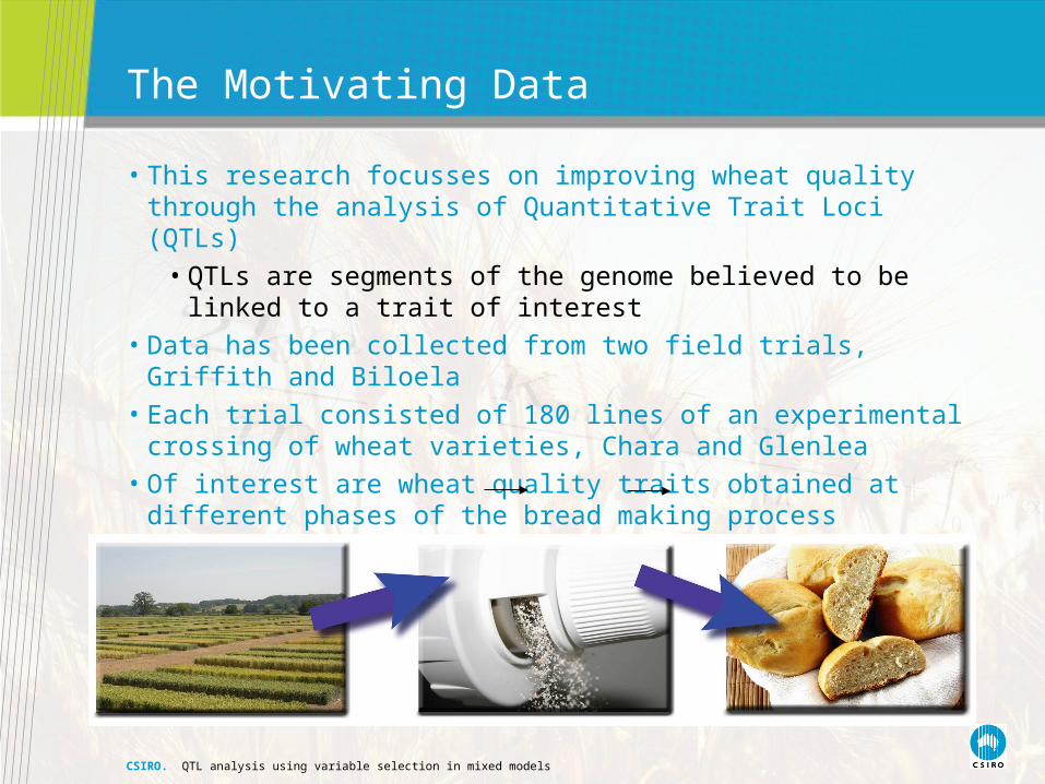
• This research focusses on improving wheat quality through the analysis of Quantitative Trait Loci (QTLs)

• QTLs are segments of the genome believed to be linked to a trait of interest

• Data has been collected from two field trials, Griffith and Biloela

• Each trial consisted of 180 lines of an experimental crossing of wheat varieties, Chara and Glenlea

• Of interest are wheat quality traits obtained at different phases of the bread making process

• For example , Field Trial Milling Baking


The Motivating Data

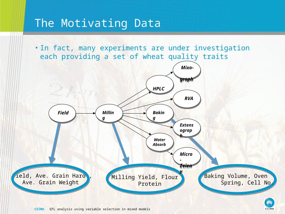
• In fact, many experiments are under investigation each providing a set of wheat quality traits

Yield, Ave. Grain Hard., Ave. Grain Weight

Milling Yield, Flour Protein

Baking Volume, Oven Spring, Cell No.

Milling

Milling

Field Field

Mixo- graph

Mixo- graph

WaterAbsorb

WaterAbsorb

RVA RVA

Baking

Baking

HPLC

HPLC

Extensograph

Extensograph

Micro-Zeleny

Micro-Zeleny


The Motivating Data

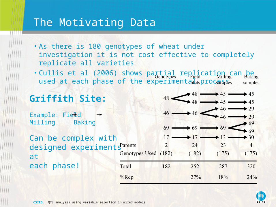
• As there is 180 genotypes of wheat under investigation it is not cost effective to completely replicate all varieties

• Cullis et al (2006) shows partial replication can be used at each phase of the experimental process

Griffith Site:

Example: Field Milling Baking

Can be complex with designed experiments ateach phase!


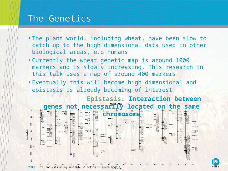
• The plant world, including wheat, have been slow to catch up to the high dimensional data used in other biological areas, e.g humans

• Currently the wheat genetic map is around 1000 markers and is slowly increasing. This research in this talk uses a map of around 400 markers

• Eventually this will become high dimensional and epistasis is already becoming of interest

Epistasis: Interaction between genes not necessarily located on the same chromosome

The Genetics


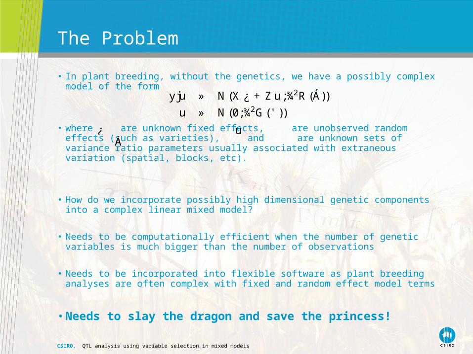
• In plant breeding, without the genetics, we have a possibly complex model of the form

• where are unknown fixed effects, are unobserved random effects (such as varieties), and are unknown sets of variance ratio parameters usually associated with extraneous variation (spatial, blocks, etc).

• How do we incorporate possibly high dimensional genetic components into a complex linear mixed model?

• Needs to be computationally efficient when the number of genetic variables is much bigger than the number of observations

• Needs to be incorporated into flexible software as plant breeding analyses are often complex with fixed and random effect model terms

• Needs to slay the dragon and save the princess!

The Problem

yju » N (X ¿ +Zu;¾2R (Á))

u » N (0;¾2G(' ))

¿ uÁ '


Mixed Model Variable Selection (MMVS):Epistatic Working Model

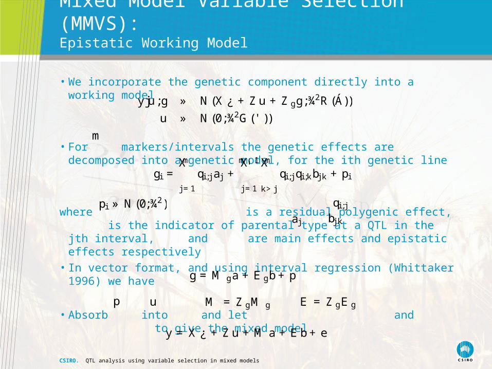
• We incorporate the genetic component directly into a working model

• For markers/intervals the genetic effects are decomposed into a genetic model, for the ith genetic line

where is a residual polygenic effect, is the indicator of parental type at a QTL in the jth interval, and are main effects and epistatic effects respectively

• In vector format, and using interval regression (Whittaker 1996) we have

• Absorb into and let and to give the mixed model

yju;g » N (X ¿ +Zu +Z gg;¾2R (Á))

u » N (0;¾2G(' ))

gi =mX

j =1

qi ;j aj +m¡ 1X

j =1

mX

k>j

qi ;j qi ;kbj k +pi

pi » N (0;¾2) qi ;jaj bj k

g =M ga +E gb+p

p u M =Z gM g E = Z gE g

y = X ¿ +Zu +M a +E b+e

m


MMVS: Variable Selection Distribution

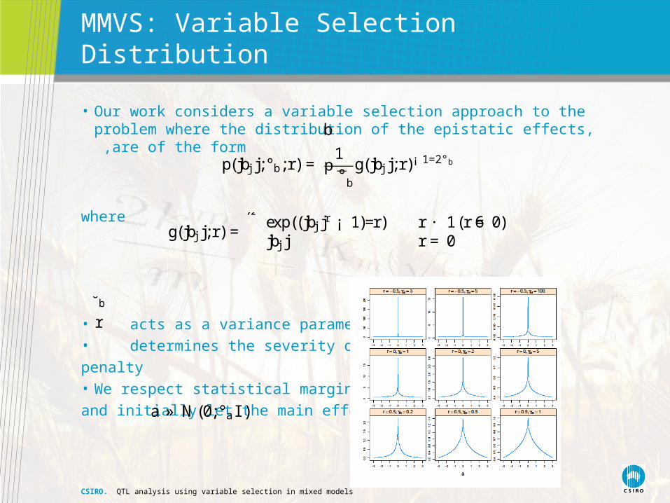
• Our work considers a variable selection approach to the problem where the distribution of the epistatic effects, ,are of the form

where

• acts as a variance parameter • determines the severity of the

penalty• We respect statistical marginality

and initially let the main effects be

b

p(jbj j;°b;r) =1p°bg(jbj j;r)¡ 1=2°b

g(jbj j; r) =½exp((jbj jr ¡ 1)=r) r · 1(r 6= 0)jbj j r = 0

°br

a » N (0;°aI )


MMVS: Estimation

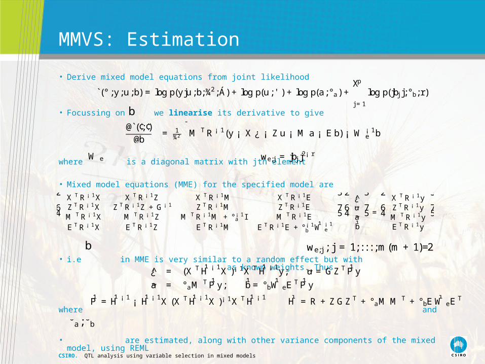
• Derive mixed model equations from joint likelihood

• Focussing on we linearise its derivative to give

where is a diagonal matrix with jth element

• Mixed model equations (MME) for the specified model are

• i.e in MME is very similar to a random effect but with as known weights. Thus

where and

• are estimated, along with other variance components of the mixed model, using REML

2

64

X T R ¡ 1X X T R ¡ 1Z X T R ¡ 1M X T R ¡ 1EZ T R ¡ 1X Z T R ¡ 1Z +G ¡ 1 Z T R ¡ 1M Z T R ¡ 1EM T R ¡ 1X M T R ¡ 1Z M T R ¡ 1M +° ¡ 1a I M T R ¡ 1EE T R ¡ 1X E T R ¡ 1Z E T R ¡ 1M E T R ¡ 1E +° ¡ 1b ¹W ¡ 1

e

3

75

2

64

¿̂~u~a¹b

3

75 =

2

64

X T R ¡ 1yZ T R ¡ 1yM T R ¡ 1yE T R ¡ 1y

3

75

W e

b we;j ; j = 1;: : : ;m(m+1)=2

°a;°b

¿̂ = (X T ¹H ¡ 1X )¡ 1X T ¹H ¡ 1y; ~u =GZ T ¹P y

~a = °aMT ¹P y; ¹b= °b ¹W eE

T ¹P y

¹P = ¹H ¡ 1 ¡ ¹H ¡ 1X (X T ¹H ¡ 1X )¡ 1X T ¹H ¡ 1 ¹H = R +ZGZ T +°aM MT +°bE ¹W eE

T

(̀° ;y;u;b) = log p(yju;b;¾2;Á) + log p(u;' ) + log p(a;°a) +pX

j =1

log p(jbj j;°b; r)

@̀(¢;¢)@b

= 1¾2

³M TR ¡ 1(y ¡ X ¿ ¡ Zu ¡ M a ¡ E b) ¡ W ¡ 1

e b´

we;j = jbj j2¡ r

b


MMVS: Dimension Reduction

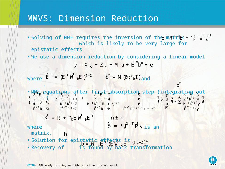
• Solving of MME requires the inversion of the matrix which is likely to be very large for epistatic effects

• We use a dimension reduction by considering a linear model

where and .

• MME equations after first absorption step (integrating out )

where is an matrix.

• Solution for epistatic effects is

• Recovery of is found by back transformation

E TR ¡ 1E +°¡ 1b ¹W ¡ 1e

y = X ¿ +Zu +M a + ¹E ¤b¤+e

¹E ¤ = (E T ¹W eE )1=2 b¤ » N (0;°bI )

2

664

X T ¹K ¡ 1X X T ¹K ¡ 1Z X T ¹K ¡ 1M 0Z T ¹K ¡ 1X Z T ¹K ¡ 1Z +G ¡ 1 Z T ¹K ¡ 1M 0M T ¹K ¡ 1X M T ¹K ¡ 1Z M T ¹K ¡ 1M +° ¡ 1a I 0¹E ¤T R ¡ 1X ¹E ¤T R ¡ 1Z ¹E ¤T R ¡ 1M ¹E ¤T R ¡ 1E ¤ +° ¡ 1b I

3

775

2

64

¿̂~u~a¹b¤

3

75 =

2

664

X T ¹K ¡ 1yZ T ¹K ¡ 1yM T ¹K ¡ 1y¹E T R ¡ 1y

3

775

¹K = R +°bE ¹W eET n£ n

¹b¤= °b ¹E

¤T ¹P y

b

¹b= ¹W eET (E ¹W eE

T )¡ 1=2¹b¤

b¤


MMVS: Working Model Algorithm

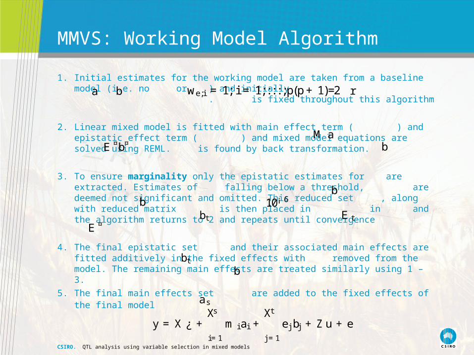
1. Initial estimates for the working model are taken from a baseline model (i.e. no or ) and initially . is fixed throughout this algorithm

2. Linear mixed model is fitted with main effect term ( ) and epistatic effect term ( ) and mixed model equations are solved using REML. is found by back transformation.

3. To ensure marginality only the epistatic estimates for are extracted. Estimates of falling below a threshold, are deemed not significant and omitted. This reduced set , along with reduced matrix is then placed in in and the algorithm returns to 2 and repeats until convergence

4. The final epistatic set and their associated main effects are fitted additively in the fixed effects with removed from the model. The remaining main effects are treated similarly using 1 – 3.

5. The final main effects set are added to the fixed effects of the final model

we;i =1; i = 1;:: : ;p(p+1)=2

M a

b

E ¤b¤

a

as

bb 10¡ 6

bt

btb

y = X ¿ +sX

i=1

m iai +tX

j =1

ej bj +Zu +e

r

b

E tE ¤


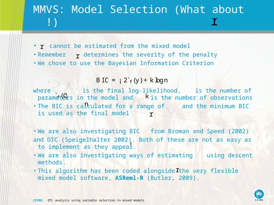
MMVS: Model Selection (What about !)

• cannot be estimated from the mixed model

• Remember determines the severity of the penalty

• We chose to use the Bayesian Information Criterion

where is the final log-likelihood, is the number of parameters in the model and is the number of observations

• The BIC is calculated for a range of and the minimum BIC is used as the final model

• We are also investigating BIC from Broman and Speed (2002)

and DIC (Speigelhalter 2002). Both of these are not as easy as to implement as they appear.

• We are also investigating ways of estimating using descent methods.

• This algorithm has been coded alongside the very flexible mixed model software, ASReml-R (Butler, 2009).

rr

BI C = ¡ 2̀ f (y) +k logn

f̀ (¢) kn

r

r

±

r


Simulations (Main Effects)

• Low dimensional study

• 9 chromosomes with 11 markers equally spaced 10cM apart

• 7 QTLs simulated with locations at midpoints of • Chr 1, Interval 4; Chr 1, Interval 8 (Repulsion)• Chr 2, Interval 4; Chr 2, Interval 8 (Coupling)• Chr 3, Interval 6• Chr 4, Interval 4• Chr 5, Interval 1

• All simulated with size 0.38 (Chr 1, Interval 8 has size -0.38)

• 1000 simulations for population sizes 100,200 and 400 were analysed

• WGAIM (Verbyla et al, 2007) and new Mixed Model Variable Selection, MMVS, methods were used for analysis

• WGAIM outperforms CIM quite considerably across all population sizes and so CIM is not presented here


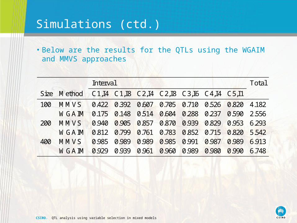
Simulations (ctd.)

• Below are the results for the QTLs using the WGAIM and MMVS approaches

Interval Total

Size Method C1,I4 C1,I8 C2,I4 C2,I8 C3,I6 C4,I4 C5,I1

100 MMVS 0.422 0.392 0.607 0.705 0.710 0.526 0.820 4.182WGAIM 0.175 0.148 0.514 0.604 0.288 0.237 0.590 2.556

200 MMVS 0.940 0.905 0.857 0.870 0.939 0.829 0.953 6.293WGAIM 0.812 0.799 0.761 0.783 0.852 0.715 0.820 5.542

400 MMVS 0.985 0.989 0.989 0.985 0.991 0.987 0.989 6.913WGAIM 0.929 0.939 0.961 0.960 0.989 0.980 0.990 6.748


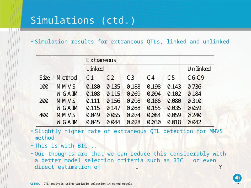
Simulations (ctd.)

• Simulation results for extraneous QTLs, linked and unlinked

• Slightly higher rate of extraneous QTL detection for MMVS method

• This is with BIC ..

• Our thoughts are that we can reduce this considerably with a better model selection criteria such as BIC or even direct estimation of

Extraneous

Linked Unlinked

Size Method C1 C2 C3 C4 C5 C6-C9

100 MMVS 0.180 0.135 0.188 0.198 0.143 0.736WGAIM 0.108 0.115 0.069 0.094 0.102 0.184

200 MMVS 0.111 0.156 0.098 0.186 0.080 0.310WGAIM 0.115 0.147 0.088 0.155 0.035 0.059

400 MMVS 0.049 0.055 0.074 0.084 0.059 0.240WGAIM 0.045 0.044 0.028 0.030 0.018 0.042

± r


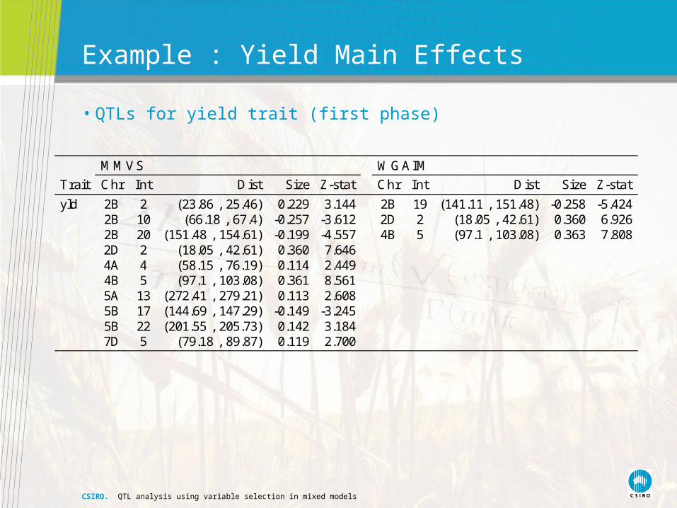
Example : Yield Main Effects

• QTLs for yield trait (first phase)

MMVS WGAIM

Trait Chr Int Dist Size Z-stat Chr Int Dist Size Z-stat

yld 2B 2 (23.86 , 25.46) 0.229 3.144 2B 19 (141.11 , 151.48) -0.258 -5.4242B 10 (66.18 , 67.4) -0.257 -3.612 2D 2 (18.05 , 42.61) 0.360 6.9262B 20 (151.48 , 154.61) -0.199 -4.557 4B 5 (97.1 , 103.08) 0.363 7.8082D 2 (18.05 , 42.61) 0.360 7.6464A 4 (58.15 , 76.19) 0.114 2.4494B 5 (97.1 , 103.08) 0.361 8.5615A 13 (272.41 , 279.21) 0.113 2.6085B 17 (144.69 , 147.29) -0.149 -3.2455B 22 (201.55 , 205.73) 0.142 3.1847D 5 (79.18 , 89.87) 0.119 2.700


Example: Cell No. Main Effects

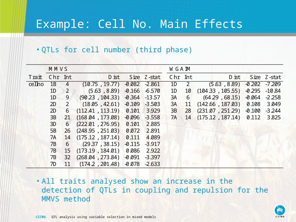
• QTLs for cell number (third phase)

• All traits analysed show an increase in the detection of QTLs in coupling and repulsion for the MMVS method

MMVS WGAIM

Trait Chr Int Dist Size Z-stat Chr Int Dist Size Z-statcellno 1B 4 (10.75 , 19.77) -0.082 -2.861 1D 2 (5.63 , 8.89) -0.202 -7.209

1D 2 (5.63 , 8.89) -0.166 -6.570 1D 10 (104.33 , 105.55) -0.295 -10.841D 9 (90.23 , 104.33) -0.364 -13.57 3A 6 (64.29 , 68.15) -0.064 -2.2582D 2 (18.05 , 42.61) -0.109 -3.503 3A 11 (142.66 , 187.03) 0.108 3.0492D 6 (112.41 , 113.19) 0.101 3.929 3B 28 (231.07 , 251.29) -0.100 -3.2443B 21 (168.04 , 173.08) -0.096 -3.558 7A 14 (175.12 , 187.14) 0.112 3.8253D 6 (222.01 , 276.95) 0.101 2.8855B 26 (248.95 , 251.03) 0.072 2.8917A 14 (175.12 , 187.14) 0.111 4.0897B 6 (29.37 , 38.15) -0.115 -3.9177B 15 (173.19 , 184.01) 0.086 2.9227B 32 (268.04 , 273.84) -0.091 -3.3977D 11 (174.2 , 201.48) -0.078 -2.633


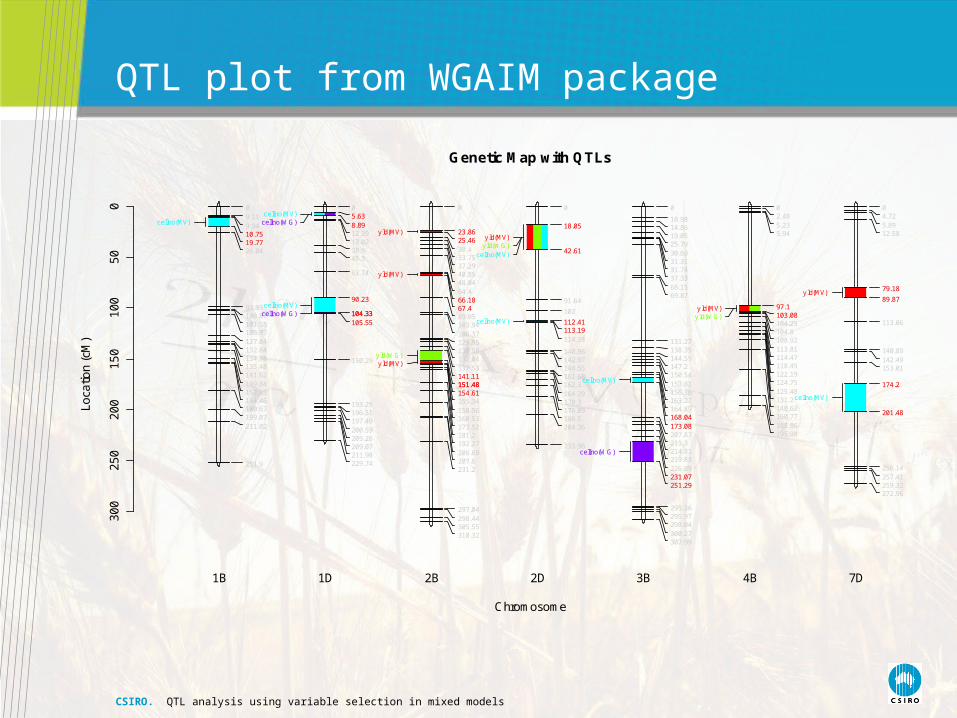
QTL plot from WGAIM package

Chromosome

Lo

catio

n (

cM)

30

02

50

20

01

50

10

05

00 0

9.119.9410.7519.7726.04

97.93100.87101.58106.37127.04132.84134.78135.48141.62149.84152.83154.46180.67199.07211.02

251.9

05.638.8912.3913.0238.945.3

63.74

90.23

104.33105.55

150.29

193.29196.51197.49200.59205.26209.07211.98229.74

0

23.8625.4630.433.7537.2940.8548.0464.466.1867.489.05103.94106.37129.95130.58132.04137.53141.11151.48154.61155.34158.56160.53173.52181.2192.27206.69207.6231.2

297.04298.44305.55310.32

0

18.05

42.61

91.64

102

112.41113.19114.38

140.96142.97144.55161.68162.3164.29170.3176.09186.5204.36

233.96

0

10.9814.8619.0525.7930.6931.3131.7437.3368.1569.87

131.27138.35144.59147.2150.54153.82156.36163.27164.89168.04173.08207.87211.3214.81219.83226.09231.07251.29

295.36295.97298.04300.27307.99

02.485.235.94

97.1103.08104.25104.8108.92113.81114.47118.45122.19124.75125.48131.2140.62160.77185.86195.94

04.725.8912.58

79.18

89.87

113.06

140.89142.49153.01

174.2

201.48

256.14257.41259.32272.96

1B 1D 2B 2D 3B 4B 7D

10.7519.77

cellno(MV)5.638.89

cellno(MV)cellno(WG)

90.23

104.33cellno(MV)

104.33105.55

cellno(WG)

23.8625.46

y ld(MV)

66.1867.4

y ld(MV)

141.11151.48

y ld(WG)

151.48154.61

y ld(MV)

18.05

42.61

y ld(MV)y ld(WG)

cellno(MV)

112.41113.19

cellno(MV)

168.04173.08

cellno(MV)

231.07251.29

cellno(WG)

97.1103.08

y ld(MV)y ld(WG)

79.18

89.87y ld(MV)

174.2

201.48

cellno(MV)

Genetic Map with QTLs


Summary and Future Work

• New MMVS method we can incorporate high dimensional data into complex mixed models in a natural way

• This is not restricted to statistical genetics!

• R package is coming shortly

• The method is general and so opens the door for high dimensional analysis in other areas requiring complex mixed models

Future work:

• A methods epistatic interactions paper is in prep. which will highlight the difficulty with finding these effects

• QTL mapping with multi-way crosses using WGAIM and MMVS is in progress


As Rove calls it ….

Here comes ….

The Plug!

1) Taylor, J. D and Verbyla, A. P (2009) A variable selection method for the analysis of QTLs in complex linear mixed models, Finalised.

2) Taylor, J. D and Verbyla, A. P (2009) High dimensional analysis of QTLs in complex linear mixed models, In Preparation.

3) Taylor, J. D and Verbyla, A. P (2009) Efficient variable selection using the normal-inverse gamma specification, Journal of Computational and Graphical Statistics, Submitted.

4) Cavanagh, C. R and Taylor, J. D et al. (2009) Sponge and dough bread making: genetic and phenotypic correlations of sponge wheat quality traits, Theoretical and Applied Genetics, Submitted.

Contact UsPhone: 1300 363 400 or +61 3 9545 2176

Email: [email protected] Web: www.csiro.au

Say hi to your mum for me!

CMIS/AgribusinessJulian TaylorPostdoctoral Fellow

Phone: 08 8303 8792Email: [email protected]: www.cmis.csiro.au

CMIS/AgribusinessAri VerbylaProfessor

Phone: 08 8303 8769Email: [email protected]: www.cmis.csiro.au

whole genome qtl analysis using variable selection in complex linear mixed models julian taylor...

Documents