Why Are Older Women Missing in India?

The Age Profile of Bargaining Power and Poverty

Rossella Calvi?

Boston College

JOB MARKET PAPER

November, 2015†

Abstract

The ratio of women to men is particularly low in India relative to developed countries. It has re-

cently been argued that close to half of these missing women are of post-reproductive ages (45 and

above), but what drives this phenomenon remains unclear. I provide an explanation for this puzzle

that is based on intra-household bargaining and resource allocation. I use both reduced-form and

structural modeling to establish the critical connections between women’s bargaining position within

the household, their health, and their age. First, using amendments to the Indian inheritance law

as a natural experiment, I demonstrate that improvements in women’s bargaining position within

the household lead to better health outcomes. Next, with a structural model of Indian households, I

show that women’s bargaining power and their ability to access household resources deteriorate at

post-reproductive ages. Thus, at older ages poverty rates are significantly higher among women than

men. My analysis indicates that gender inequality within the household and the consequent gender

asymmetry in poverty can account for up to 82 percent of missing women of post-reproductive ages.

Finally, I demonstrate that policies aimed at promoting intra-household equality, such as improving

women’s rights to inherit property, can have a large impact on female poverty and mortality.

Keywords: missing women, intra-household bargaining power, women’s health, Hindu Succession

Act, collective model, resource shares, poverty, elderly.

JEL codes: D1, K36, I12, I31, I32, J12, J14, J16.

?Boston College, Department of Economics, Chestnut Hill, MA 02467. Email: rossella.calvi@bc.edu.I am grateful to Arthur Lewbel, Scott Fulford, and Andrew Beauchamp for their guidance, advice and continued support. I thank SamsonAlva, S Anukriti, Samuel Bazzi, Donald Cox, Zaichao Du, Alexander Eiermann, Christopher Hale, Larry Iannaccone, Lisa Lynch, FedericoMantovanelli, Dilip Mookherjee, Anant Nyshadham, Claudia Olivetti, Sarmistha Pal, Yong-Hyun Park, Debraj Ray, Tracy Regan, David Schenck,Fabio Schiantarelli, Meghan Skira, Denni Tommasi, Alessandra Voena, and all participants at the Boston College Applied Micro Workshop, at theBoston College Dissertation Workshop, at the 2015 ASREC Graduate Workshop at Chapman University, at the Boston University DevelopmentReading Group, at the 2015 EGS Conference at Washington University, and at the 2015 NEUDC Conference at Brown University for theirsuggestions and insight. I would also like to thank the Boston College Institute on Aging for supporting this project. All errors are my own.

†First Draft: March, 2015. Latest version available at www2.bc.edu/rossella-calvi.

1 Introduction

There are far more men than women in India relative to developed countries. Following seminal

work by Amartya Sen (1990; 1992), this fact has been dubbed the missing women phenomenon.1

Sex-selective abortion and excess female mortality at early ages related to parental preferences

for sons have been identified as important determinants of missing women and biased sex-ratios.2

Recent work by Anderson and Ray, however, indicates that excess female mortality in India persists

beyond childhood and that the majority of missing Indian women die in adulthood. While they do

not dispute the presence of a severe gender bias at young ages and the role played by maternal

mortality, Anderson and Ray (2010) demonstrate that close to half of missing women in India are

of post-reproductive ages, i.e., 45 and above (see figure 1).3 Unlike the missing girls phenomenon,

excess female mortality at older ages in India has not received much attention and remains a

puzzle.

I seek to explain this puzzle by examining the critical connections between women’s age, intra-

household bargaining, and health, while taking the link between health and mortality as given.

Using reduced-form and structural methods, I identify one crucial mechanism – the decline in

women’s bargaining position during post-reproductive ages – that can account for 82 percent of

the missing women in the 45-79 age group. The decrease in women’s bargaining power is reflected

in their diminished ability to access household resources. As a consequence, at older ages poverty

rates are significantly higher among women than men. I call this fact excess female poverty and

show that the age profile of excess female poverty matches the profile of excess female mortality in

figure 1 nearly exactly at post-reproductive ages.

My analysis proceeds in two steps. First, by using amendments to the Indian inheritance law

as a natural experiment, I analyze the relationship between women’s bargaining power and their

health. I focus on the Hindu Succession Act (HSA) amendments that equalized women’s inheri-

tance rights to men’s in several Indian states between 1976 and 2005. Using data from the 2005-

2006 National Family Health Survey (NFHS-3), I show that women’s exposure to these reforms

increases their body mass index and reduces the probability of them being anaemic or underweight

by strengthening their bargaining power. Next, I examine whether older women are missing in

India because their bargaining position weakens at post-reproductive ages. To test my hypothesis,

I set out a household model with efficient bargaining to structurally estimate women’s bargaining

power and investigate its determinants. At post-reproductive ages, I find evidence of a substantial

decline in women’s bargaining position and in their ability to access household resources.

1Coale (1991) estimates that over 23 million of Indian women who should be alive are missing.2See e.g., Sen (1990) and DasGupta (2005).3They estimate a total of 1.7 million excess female deaths in year 2000 alone (0.34 percent of the total female population), 45 percent of

which occurred at the age of 45 and above. In contrast, they find that close to 44 percent of China’s missing women are located “around birth".For each age category, Anderson and Ray (2010) compare the actual female death rate in India to a reference female death rate. The latter isone that would be obtained if the death rate of males in India were to be rescaled by the relative death rates for males and females (in the samecategory) in developed countries. They compute missing women as the product between the difference between the actual and reference deathrates and the female population in each age group. Figure 1 displays estimates from Anderson and Ray (2010), table 3, p. 1275. These resultsare further investigated and confirmed in Anderson and Ray (2012). These findings are consistent with a striking non-monotonic pattern ofsex-ratios over age. See section A.1 in the Appendix for more details.

1

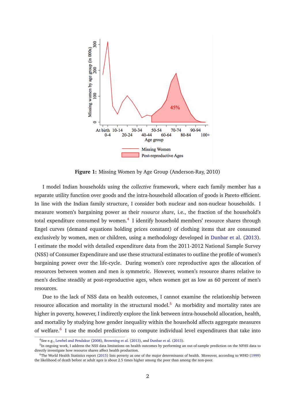
Figure 1: Missing Women by Age Group (Anderson-Ray, 2010)

I model Indian households using the collective framework, where each family member has a

separate utility function over goods and the intra-household allocation of goods is Pareto efficient.

In line with the Indian family structure, I consider both nuclear and non-nuclear households. I

measure women’s bargaining power as their resource share, i.e., the fraction of the household’s

total expenditure consumed by women.4 I identify household members’ resource shares through

Engel curves (demand equations holding prices constant) of clothing items that are consumed

exclusively by women, men or children, using a methodology developed in Dunbar et al. (2013).

I estimate the model with detailed expenditure data from the 2011-2012 National Sample Survey

(NSS) of Consumer Expenditure and use these structural estimates to outline the profile of women’s

bargaining power over the life-cycle. During women’s core reproductive ages the allocation of

resources between women and men is symmetric. However, women’s resource shares relative to

men’s decline steadily at post-reproductive ages, when women get as low as 60 percent of men’s

resources.

Due to the lack of NSS data on health outcomes, I cannot examine the relationship between

resource allocation and mortality in the structural model.5 As morbidity and mortality rates are

higher in poverty, however, I indirectly explore the link between intra-household allocation, health,

and mortality by studying how gender inequality within the household affects aggregate measures

of welfare.6 I use the model predictions to compute individual level expenditures that take into

4See e.g., Lewbel and Pendakur (2008), Browning et al. (2013), and Dunbar et al. (2013).5In ongoing work, I address the NSS data limitations on health outcomes by performing an out-of-sample prediction on the NFHS data to

directly investigate how resource shares affect health production.6The World Health Statistics report (2015) lists poverty as one of the major determinants of health. Moreover, according to WHO (1999)

the likelihood of death before at adult ages is about 2.5 times higher among the poor than among the non-poor.

2

account unequal intra-household allocation. I compare these per-capita expenditures to poverty

thresholds to calculate gender and gender-age specific poverty rates. By contrast, standard per

capita poverty measures assume equal sharing and ignore intra-household inequality. My poverty

estimates indicate that at all ages there are more women living in poverty than men, but the

gap between female and male poverty rates widens dramatically at post-reproductive ages. For

individuals aged 45 to 79, poverty rates are on average 80 percent higher among women than

men. This result provides additional support for my hypothesis that intra-household inequality can

explain excess female mortality. Using a simple model to relate my findings to the Anderson and

Ray’s estimates, I then demonstrate that a considerable proportion of missing women at older ages

can be attributed to intra-household gender inequality.

My structural estimates are consistent with the existing reduced-form evidence of the impor-

tance of inheritance rights in shaping women’s position within the household.7 I find that exposure

to the Hindu Succession Act amendments increases women’s resource shares by 0.2 standard devi-

ations. These reforms were enacted in different states at different times between 1976 and 2005

and only applied to Hindu, Buddhist, Sikh and Jain women who were not married at the time of

implementation. A large fraction of Indian women, especially of older ages, is therefore excluded.

I perform a counterfactual exercise and calculate women’s resource shares in the hypothetical sce-

nario of all women (of all religions and ages) benefiting from these reforms. I demonstrate that

granting universal equal inheritance rights can reduce the number of women living in extreme

poverty by 10 percent and the number of excess female deaths at post-reproductive ages by up to

26 percent.

The contribution of this paper is fourfold. First, this study is the first to show that excess female

mortality at older ages in India can be explained by asymmetries in intra-household bargaining

and resource allocation. While Anderson and Ray (2010, 2012) raise awareness about this phe-

nomenon, little work has been done to understand possible channels generating excess female

mortality in adulthood in India, especially at older ages. Milazzo (2014) argues that excess mor-

tality among women aged 30 to 49 could be partly explained by son preference, while a recent

working paper by Anderson and Ray (2015) shows that excess female mortality between the ages

of 20 and 65 is particularly severe among unmarried women and widows. My analysis departs from

previous works in that it provides an original explanation for missing women at older ages (45 to

79) while employing both reduced-form analysis and structural modeling. The structural model

allows me to perform counterfactual experiments and to examine the roles of son preference and

widowhood within a full model of household bargaining. Second, while the effect of changes in

Indian inheritance laws on women’s outcomes has been studied previously (e.g., Roy (2008, 2013),

Deininger et al. (2013), and Heath and Tan (2014)), no work focused explicitly on women’s health

and access to household resources. Third, this is the first attempt to formally outline the profile of

women’s intra-household bargaining power over the life-cycle in a developing country. Fourth, to

7See e.g., Roy (2008) and Heath and Tan (2014), who show that women’s exposure to the HSA reforms improves self-reported measuresof autonomy and negotiating power within their marital families.

3

the best of my knowledge, this paper is the first to provide measures of gender-age specific poverty

that take into account unequal resource allocation within the household.

Important policy implications may be drawn from this analysis. As the population in India

and in other developing countries ages, gender asymmetries among the elderly need to be fur-

ther investigated and promptly addressed. Moreover, policies aimed at promoting equality within

households, such as improving women’s rights to inherit property, can have positive spillovers on

female health, poverty and mortality. Finally, intra-household inequalities should be taken into

account when measuring poverty and evaluating the effect of policies to alleviate it.

The rest of the paper is organized as follows. Section 2 provides an overview of the related

literature and discusses further the contributions of this paper. Section 3 presents the reduced-form

results and establishes a positive causal link between women’s intra-household bargaining power

and their health. Section 4 discusses the household model, the identification of resource shares and

the structural estimation results. Section 5 outlines the age profiles of female bargaining power and

poverty and relates them to the phenomenon of excess female mortality at post-reproductive ages.

Section 6 presents the counterfactual policy analysis. Section 7 concludes.

2 Related Literature

This paper relates to several strands of literature: the previous research on the missing women

phenomenon, the existing studies on poverty among the elderly in South Asia, the work on in-

heritance rights and the Hindu Succession Act amendments in particular, and the literature on

intra-household allocation and bargaining power.

Since it was first addressed by Amartya Sen in 1990, the phenomenon of missing women has

been widely studied. It refers to the fact that in parts of the developing world, especially in India

and China, the ratio of women to men is particularly skewed. Coale (1991) estimates a total of

60 million missing females in the world at the beginning of the nineties, with India accounting for

more than one third of them. In 2010, 126 million women were missing from the global popula-

tion, with China and India accounting for 85% of this bias in sex ratios (Bongaarts and Guilmoto

(2015)). The literature has traditionally related this fact to son preference and several works have

provided empirical evidence of sex-selective abortion, female infanticide and excess female mor-

tality in childhood (see DasGupta (2005) for an overview of this literature). Jha et al. (2006) find

strong evidence of selective abortion of female fetuses in India. Moreover, the introduction of ultra-

sound technologies at the end of the 1980s has been found to be associated with even more skewed

sex-ratios and preferential prenatal treatment for boys (Bhalotra and Cochrane (2010); Bharadwaj

and Lakdawala (2013)).8 Finally, Oster (2009) and Jayachandran and Kuziemko (2011) show that

gender differences in child mortality are associated with differential health investment between

8While access to ultra-sound has reduced gender gaps in post-neonatal child mortality, Anukriti et al. (2015) demonstrate that this declineis not large enough to compensate for the increase in the male-female sex ratio at birth due to sex-selective abortions.

4

genders.9

A notable exception to this literature is the recent work by Anderson and Ray (2010; 2012;

2015), who indicate that close to half of missing women in India die at older ages. The plight

of widows in the Indian subcontinent has been previously investigated by Jean Drèze and coau-

thors in a series of papers (Drèze et al. (1990); Chen and Drèze (1995); Drèze and Srinivasan

(1997)). Moreover, previous work on the conditions of the elderly in South Asia suggests that

women’s bargaining power and access to household resources may indeed be key to explain the

phenomenon of missing women at post-reproductive ages. Kochar (1999), for example, finds that

medical expenditure on the elderly in rural Pakistan is negatively affected by their declining eco-

nomic contribution to the household. Moreover, Roy and Chaudhuri (2008) show that older Indian

women report worse self-rated health status, higher prevalence of disabilities, and lower healthcare

utilization than men. While the health disadvantage and lower utilization among women cannot

be explained by demographics, they find that gender differentials disappear when controlling for

economic independence.

Women’s bargaining power and its changes are difficult to measure and often unobservable.

Legal reforms aimed at improving women’s property rights, inheritance rights in particular, have

been widely used in the literature to assess the relationship between bargaining power and women’s

outcomes. Mine is the first paper that focuses on health outcomes, measures of undernourishment

and anaemia in particular, and on access to household resources. Deininger et al. (2013) find

evidence of an increase of women’s likelihood of inheriting land following the introduction of Hindu

Succession Act (HSA) amendments that equalized women’s inheritance rights to men’s in several

Indian states. Moreover, Roy (2008) shows that women’s exposure to the HSA reforms improves

their bargaining power and autonomy within their marital families and Roy (2013), Deininger

et al. (2013), and Bose and Das (2015) indicate that it increases female education.10 Heath and

Tan (2014) show that the HSA amendments increase women’s labor supply, especially into high-

paying jobs.11 Finally, Jain (2014) shows that HSA reforms mitigate son preference, and might be

effective in reducing mortality differences between boys and girls in rural India.12

A remarkably diverse literature has focused on intra-household resource allocation and bar-

gaining power. On one hand, several papers have tested empirically whether households behave in

9Discrimination against girls in India has also being investigated by directly looking at how household consumption patterns varies withthe gender composition of children. Most of these works use the so called Engel curve approach - not to be confused with the structuralapproach of identification of resource shares based on Engel curves estimation that I implement in this paper -, which consists on regressingbudget shares of a set of goods on log per-capita expenditure, log household size, the shares of various age-sex groups and other relevanthousehold characteristics. Among others, Subramanian and Deaton (1990) find evidence of gender discrimination in rural Maharashtra for10-14 year olds, Lancaster et al. (2008) find empirical evidence of gender bias in rural Bihar and Maharashtra for the 10-16 age group, whileZimmermann (2012) finds that gender discrimination in education expenditures between boys and girls increases with age.

10Unintended negative consequences of these reforms have been studied as well. Rosenblum (2015), for example, shows that the HSAamendments increase female child mortality, which is consistent with parents wanting to maximize their bequest per son. Anderson andGenicot (2015) show that HSA reforms are associated with a decrease in the difference between female and male suicide rates, but with anincrease in both male and female suicides.

11While analyzing possible underlying mechanisms, they also find some preliminary evidence of health improvements following the imple-mentation of HSA amendments.

12Legal reforms in other countries have been studied as well. La Ferrara and Milazzo (2014), for example, exploit an amendment to Ghana’sIntestate Succession Law and compare differential responses of matrilineal and patrilineal ethnic groups, finding that parents substitute landinheritance with children’s education. Harari (2014) analyzes a law reform meant to equalize inheritance rights for Kenyan women and showsthat women exposed to the reform are more educated, less likely to undergo genital mutilation, and have higher age at marriage and at firstchild.

5

accordance with the unitary model, which assumes that the household acts as a single decision unit

maximizing a common utility function.13 On the other hand, a number of papers have focused on

developing techniques by which household level consumption data may be used to recover infor-

mation about individual household members. Building on Chiappori (1988, 1992) and Apps and

Rees (1988), the vast majority of these studies concentrate on the estimation of collective household

models, in which the household is characterized as a collection of individuals, each of whom has

a well defined objective function, and who interact to generate Pareto efficient allocations, while

the exact intra-household bargaining protocol is left unspecified. Identification of individuals’ re-

source shares (or sharing rule), defined as each member’s share of total household consumption, is

particularly appealing, as it provides a measure of individuals’ intra-household bargaining power.

Although a series of papers focus on the identification of changes in resource shares as functions of

factors affecting bargaining power (Browning et al. (1994), Browning and Chiappori (1998), Ver-

meulen (2002)), a more recent strand of the literature deals with the identification of the level of

resource shares, which is my main object of interest (Lewbel and Pendakur (2008), Browning et al.

(2013), Dunbar et al. (2013)). Dunbar et al. (2013), for example, identify individuals’ resource

shares using Engel curves of assignable clothing and find that Malawian children have higher rates

of poverty than their parents, despite commanding a quite large share of household resources.

With few exceptions, limited work has used this type of approach to investigate intra-household

allocation at older ages.14 To my knowledge, no previous work has investigated the age profile of

women’s intra-household bargaining power and its implications for poverty in a developing country.

3 Bargaining Power and Health: A Reduced-Form Analysis

While plausible, that an increase in the bargaining power of women inside the household positively

affects their health outcomes is not an obvious fact. Women, for example, may divert resources to

children when their position improves, so that no effect could be detected on their own health.

A woman’s right to inherit land and other property is often claimed to be a significant deter-

minant of women’s economic security and position within the household (World Bank (2014)). I

investigate the existence of a causal positive effect of intra-household bargaining power on women’s

health by exploiting legal reforms equalizing women’s inheritance rights to men’s. I compare health

outcomes of women who were exposed to these reforms to those of women who were not. Research

in the medical field indicates that low body mass index (BMI), especially BMI below the under-

weight cutoff of 18.5, and anaemia are associated with an increased risk of mortality.15 Evidence of

13Most of this empirical literature focus on testing the income pooling hypothesis, i.e., that only household income matters for choice outcomesand not the source of the income. See e.g., Attanasio and Lechene (2002), who examine the effect of large cash transfers in rural Mexico(PROGRESA/Oportunidades conditional cash transfers), and Duflo (2003), who analyzes a reform in the South Africa social pension programfor the elderly. They both find empirical evidence against the unitary model.

14To analyze how intra-household allocation is affected by retirement and health status of elderly in the US, Bütikofer et al. (2010) estimatea collective model with data on married couples and widows/widowers between ages 50 and 80. Cherchye et al. (2012b) analyze consumptionpattern of Dutch elderly households between 1978 and 2004 and find that traditional poverty rates seem to underestimate poverty amongwidows.

15See e.g Visscher et al. (2000), Thorogood et al. (2003), and Zheng et al. (2011).

6

improvements in these health outcomes following an increase in women’s bargaining power would

provide empirical validation to my hypothesis that intra-household resource allocation can explain

excess female mortality.

Inheritance rights in India differ by religion and, for most of the population, are governed by

the Hindu Succession Act (HSA). The HSA was first introduced in 1956 and applied to all states

other than Jammu and Kashmir and only to Hindus, Buddhists, Sikhs and Jains. It therefore did not

apply to individuals of other religions, such as Muslims, Christians, Parsis, Jews, and other minority

communities.16 It aimed at unifying the traditional Mitakhshara and Dayabhaga systems, which

were completely biased in favor of sons (Agarwal (1995)), and established a law of succession

whereby sons and daughters would enjoy (almost) equal inheritance rights, as would brothers and

sisters. Gender inequalities, however, persisted even after the introduction of the HSA. On one

hand, in case of a Hindu male dying intestate, i.e., without leaving a will, all his separate or self-

acquired property, devolved equally upon sons, daughters, widow, and mother. On the other hand,

the deceased’s daughters had no direct inheritance rights to joint family property, whereas sons

were given direct right by birth to belong to the coparcenary.17

The Indian constitution states that both federal and state governments have legislative power

over inheritance. In the decades following the introduction of Hindu Succession Act, state govern-

ments enacted amendments equalizing inheritance rights for daughters and sons. Kerala in 1976,

Andhra Pradesh in 1986, Tamil Nadu in 1989, and Maharashtra and Karnataka in 1994 passed

reforms making daughters coparceners. These reforms only applied to Hindu, Buddhist, Sikh or

Jain women, who were not yet married at the time of the amendment. A national-level ratification

of the amendments occurred in 2005.

To study the link between women’s bargaining position and health, I consider the following

baseline specification:

yirsc = βHSAA Exposedirsc + X ′irscγ+αr +αc +αs +αrs +αrc +αsc + εirsc (1)

where yirsc is the outcome of interest for woman i, of religion r, living in state s and born in year

c (BMI or an indicator variable for being underweight or severely, moderately or mildly anemic).

HSAA Exposedirsc is an indicator variable equal to one if woman i got married after the amendment

in state s and is Hindu, Buddhist, Sikh or Jain. X ′irsc is a vector of individual and household level

covariates, including women’s education, number of children in the household, a household wealth

index, and indicator variables for having worked in the past year, for living in rural areas and for

being part of disadvantaged social groups. The model includes cohort and state fixed effects,

a religion dummy equal to 1 if a woman is Hindu, Buddhist, Sikh or Jain, and zero otherwise,

16While most laws for Christians formally grant equal rights from 1986, gender equality is not the practice, as the Synod of ChristianChurches has being arranging legal counsel to help draft wills to disinherit female heirs. The inheritance rights of Muslim women in India aregoverned by the Muslim Personal Law (Shariat) Application Act of 1937, under which daughters inherit only a portion of what the sons do(Agarwal (1995)).

17All persons who acquired interest in the joint family property by birth are said to belong to the coparcenary. The Hindu Women’s Right toProperty Act of 1937 enabled the widow to succeed along with the son and to take a share equal to that of the son. The widow was entitledonly to a limited estate in the property of the deceased with a right to claim partition. A daughter, however, had virtually no inheritance rights.

7

and religion-cohort, cohort-state, and state-religion fixed effects.18 β is the parameter of interest

and represents the treatment effect of being exposed to HSA amendments, i.e., to an exogenous

variation in women’s intra-household bargaining power. In the baseline specification, standard

errors are clustered at the primary sampling unit (village) level. Results are robust to clustering

the standard errors at the state, cohort-state, and at the cohort-state-religion level.

I estimate the model via OLS using a sample of married women of age 15 to 49 from the 2005-

2006 National Family Health Survey (NFHS-3). The average body mass index in the estimation

sample lies within the normal range (18.5 to 23). Nonetheless, 26 percent of the women in the

sample is underweight. Moreover, anaemia appears to be an endemic problem, with 50 percent

of women in the sample suffering from mild anaemia, 16 percent from moderate anaemia and 2

percent from severe anaemia.19 Finally, one out of six women in the sample have been exposed to

the HSA amendments.

Table 1 presents the estimation results. The first three columns focus on BMI outcomes, over the

full sample (column 1), a sample restricted to women considered underweight or normal weight

according to the WHO cutoffs (column 2), and a sample restricted to women overweight and obese

(column 3). The sample breakdown aims at addressing potential concerns related to the non-

monotonicity of the relationship between BMI and health: while increases in BMI correspond to

better health for individuals below the overweight cutoff, the opposite holds true for individuals

above it. Exposure to HSA amendments is associated with an increase in women’s BMI by 0.15

when the entire sample is considered, and by 0.25 when only underweight and normal weight

range individuals are included. As expected, no significant effect can be detected when only over-

weight and obese women are included in the analysis. Column 4 to 7 report the linear probability

models estimation results. All specifications indicate that women exposed to HSA amendments

have better health outcomes, as they are 4 percent less likely to be underweight, about 1 percent

less likely to be severely anaemic, 3 percent less likely to be moderately anaemic, and 3 percent

less likely to be mildly anaemic.20

I perform a series of robustness checks to test the sensitivity of the reduced-form results. First,

as exposure to the HSA amendments is determined by each woman’s year of marriage, I address

concerns about the potential endogeneity of treatment by excluding from the analysis women who

got married right around the reforms, by estimating an intent-to-treat effect using a measure of

eligibility to HSA amendments that exploits variation in women’s year of birth, religion and state,

and by using an instrumental variable approach. I show that the potential endogeneity of the time

of marriage is not the driving force behind my findings. Second, I assess how exposure to HSA

amendments by the wife of the head of household affects expenditure patterns. I show that my

18The fixed effects are based on 28 states, 35 cohorts and 2 religious categories.19Section A.3 contains more details on the data and on the use of BMI and anaemia as health measures. Table A4 presents some descriptive

statistics.20To address the well known limitations of linear probability models, I estimate a maximum-likelihood probit model. Table A2 in the

Appendix shows the marginal effects of being exposed to HSA amendments on binary health outcomes. The marginal effects are computed atthe average value of the independent variables. As the number of observation is much larger than the number of fixed effects the incidentalparameter problem associated with estimating a probit model with fixed effects may be limited (Greene et al. (2002), Fernández-Val (2009)).Results are unchanged.

8

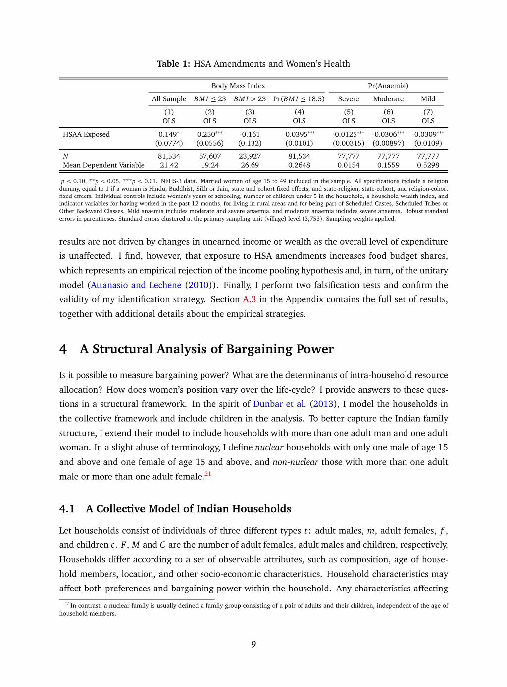
Table 1: HSA Amendments and Women’s Health

Body Mass Index Pr(Anaemia)

All Sample BM I ≤ 23 BM I > 23 Pr(BM I ≤ 18.5) Severe Moderate Mild

(1) (2) (3) (4) (5) (6) (7)OLS OLS OLS OLS OLS OLS OLS

HSAA Exposed 0.149∗ 0.250∗∗∗ -0.161 -0.0395∗∗∗ -0.0125∗∗∗ -0.0306∗∗∗ -0.0309∗∗∗

(0.0774) (0.0556) (0.132) (0.0101) (0.00315) (0.00897) (0.0109)

N 81,534 57,607 23,927 81,534 77,777 77,777 77,777Mean Dependent Variable 21.42 19.24 26.69 0.2648 0.0154 0.1559 0.5298

p < 0.10, **p < 0.05, ***p < 0.01. NFHS-3 data. Married women of age 15 to 49 included in the sample. All specifications include a religiondummy, equal to 1 if a woman is Hindu, Buddhist, Sikh or Jain, state and cohort fixed effects, and state-religion, state-cohort, and religion-cohortfixed effects. Individual controls include women’s years of schooling, number of children under 5 in the household, a household wealth index, andindicator variables for having worked in the past 12 months, for living in rural areas and for being part of Scheduled Castes, Scheduled Tribes orOther Backward Classes. Mild anaemia includes moderate and severe anaemia, and moderate anaemia includes severe anaemia. Robust standarderrors in parentheses. Standard errors clustered at the primary sampling unit (village) level (3,753). Sampling weights applied.

results are not driven by changes in unearned income or wealth as the overall level of expenditure

is unaffected. I find, however, that exposure to HSA amendments increases food budget shares,

which represents an empirical rejection of the income pooling hypothesis and, in turn, of the unitary

model (Attanasio and Lechene (2010)). Finally, I perform two falsification tests and confirm the

validity of my identification strategy. Section A.3 in the Appendix contains the full set of results,

together with additional details about the empirical strategies.

4 A Structural Analysis of Bargaining Power

Is it possible to measure bargaining power? What are the determinants of intra-household resource

allocation? How does women’s position vary over the life-cycle? I provide answers to these ques-

tions in a structural framework. In the spirit of Dunbar et al. (2013), I model the households in

the collective framework and include children in the analysis. To better capture the Indian family

structure, I extend their model to include households with more than one adult man and one adult

woman. In a slight abuse of terminology, I define nuclear households with only one male of age 15

and above and one female of age 15 and above, and non-nuclear those with more than one adult

male or more than one adult female.21

4.1 A Collective Model of Indian Households

Let households consist of individuals of three different types t: adult males, m, adult females, f ,

and children c. F , M and C are the number of adult females, adult males and children, respectively.

Households differ according to a set of observable attributes, such as composition, age of house-

hold members, location, and other socio-economic characteristics. Household characteristics may

affect both preferences and bargaining power within the household. Any characteristics affecting

21In contrast, a nuclear family is usually defined a family group consisting of a pair of adults and their children, independent of the age ofhousehold members.

9

bargaining power and how resources are allocated within the household, but neither preferences

nor budget constraints, are defined as distribution factors (Browning et al. (2014)). For simplicity

of notation, I omit household characteristics and distribution factors while discussing the model

and identification.

Each household consumes K types of goods with prices p = (p1, ..., pK). Household total expen-

diture y is set equal to household income, so there is no borrowing or lending. h = (h1, ...,hK) is

the vector of observed quantities of goods purchased by each household, while x t = (x1t ..., xK

t ) is

the vector of unobserved quantities of goods consumed by an individual of type t = f , m, c. I allow

for economies of scale in consumption through a linear consumption technology, which converts

purchased quantities by the household, h, in private good equivalents, x . This specific technology

assumes the existence of a K × K matrix A such that h= A(F x f +M xm+ C xc).22

Each member has a monotonically increasing, continuously twice differentiable and strictly

quasi-concave utility function over a bundle of K goods. Let Ut(x t) be the sub-utility function of

individual of type t over her consumption. Each type t individual’s total utility may depend on the

utility of other household members, but I assume each type’s utility function to be weakly separable

over the sub-utility functions for goods. Moreover, I assume Ut(x t) to be the same for all household

members of type t, i.e., common to all adult men, all adult women and all children, respectively. As

further discussed in section 4.2, the choice of restricting the utility functions among individuals of

the same type to be the same is data driven. For the same reason, I assume that within a household

individuals of the same type are treated equally.23

Each household maximizes the Bergson-Samuelson social welfare function, U , featuring the

relative weights of the utility functions of its members:

U(U f , Um, Uc, p/y) =∑

t∈{ f ,m,c}

µt(p/y)Ut (2)

where µt(p/y) are the Pareto weights. The household program is as follows:

maxx f ,xm,xc ,h

U(U f , Um, Uc, p/y) such that h= A(F x f +M xm+ C xc)

y = h′p (3)

The solutions to this program provide the bundles of private good equivalents, x t . Pricing those

at the shadow prices A′p gives the resource share λt =Λt

T, that is the fraction of household total

resources that are devoted to each individual of type t.

22Suppose that the two members of a nuclear household with no children ride together a motorcycle and, therefore, share the consumptionof gasoline, half of the time. Then the consumption of gasoline in private good equivalents is 1.5 times the purchased quantity of gasoline atthe household level. Assuming the consumption of gasoline does not depend on consumption of other goods, the kth row of A would consist of2/3 in the kth column and zero otherwise, such that hk = 2/3(x f + xm). 2/3 represents the level of publicness of good k within the household.If the two members ride the motorcycle together all the time, Ak = 1/2. For a private good, which is never jointly consumed, Ak = 1.

23This is an admittedly strong assumption. Distinguishing between individuals of the same type would be possible only if private assignablegoods were observable for each individual within types. To the best of my knowledge, no such data is available for India. In estimation, how-ever, all the preference parameters and the resource shares are allowed to vary with a set of household characteristics, including composition.Thus, everything else equal, women’s resource shares in a household where the wife of the head of household and a daughter in law coexistwould be different from the resource shares in a household with a wife of the head of household and an unmarried daughter above 15.

10

Pareto weights are traditionally interpreted as measures of intra-household bargaining power:

the larger is the value of µt , the greater is the weight that type t members’ preferences receive

in the household program. Browning et al. (2013) show that there exists a monotonic correspon-

dence between Pareto weights and resource shares. Moreover, they argue that the latter is a more

tractable measure of bargaining power, as it is invariant to unobservable cardinalizations of the

utility functions.

Following the standard characterization of collective models, I assume the intra-household al-

location to be Pareto efficient.24 Thus, the household program can be decomposed in two steps:

the optimal allocation of resources across members and the individual maximization of their own

utility function. Conditional on knowing λt , each household member chooses x t as the bundle

maximizing Ut subject to a Lindahl type shadow budget constraint∑

k Akpk x kt = λt y .25 By substi-

tuting the indirect utility functions Vt(A′p,λt y) in equation (3), the household program simplifies

to the choice of optimal resource shares subject to the constraint that total resources shares must

sum to one.

I define a private good to be a good that does not have any economies of scale in consumption

- e.g., food - and a private assignable good to be a private good consumed exclusively by house-

hold members of known type t - e.g., women, men or children clothing. The household demand

functions for the private assignable goods, Wt , are given by:

Wt(y, p) = Tλtwt(A′p,λt y) = Λtwt(A

′p,λt y) (4)

where t = f , m, c, T = F, M , C , and wt is the demand function of each type t household member

when facing her personal shadow budget constraint.

Women’s total resource share, Λ f = Fλ f , is my main object of interest, as it represents the

share of total household expenditure consumed by women and provides a measure of the overall

bargaining power of adult females.

4.2 Identification of Resource Shares

I identify type t individuals’ resource shares using Engel curves of assignable clothing and the

methodology developed in Dunbar et al. (2013). An Engel curve describes the relationship between

the proportion of household expenditure spent on a good (budget share) and total expenditure,

holding prices constant. Dunbar et al. (2013) demonstrate that resource shares are identified

under observability of private assignable goods, semi-parametric restrictions imposing similarity

of preferences over the private assignable goods, and the assumptions that resource shares are

24See e.g., Chiappori (1988, 1992), Browning et al. (1994), Browning and Chiappori (1998), Vermeulen (2002), Lewbel and Pendakur(2008), Browning et al. (2013), and Dunbar et al. (2013). While some papers provide evidence in favor of the collective model (e.g.,Attanasio and Lechene (2014)), some others works have cast doubt on the assumption that households behave efficiently (e.g., Udry (1996)).In Appendix A.6, I use auxiliary data on singles to show that the assumption of Pareto efficiency cannot be rejected in this context.

25This result follows directly from the second welfare theorem in an economy with public goods. See Browning et al. (2013) and Browninget al. (2014) for more details.

11

independent of expenditure (at least at low levels of y).26 As I observe type-specific assignable

goods, I am only able to retrieve type-specific resource shares.

For simplicity, I assume that each household member has Muellbauer’s Piglog preferences over

assignable clothing at all levels of expenditure.27 Under this assumption, the Engel curves for these

goods are linear in the logarithm of household expenditure. In a slight abuse of notation, the

demand functions for assignable clothing can be written in Engel curve form. In each household

with children they are as follows:

Wf (y) = α fΛ f + β fΛ f ln�

Λ f y

F

�

Wm(y) = αmΛm+ βmΛm ln�

Λm yM

�

Wc(y) = αcΛc + βcΛc ln�

Λc yC

�

(5)

where Wt(y) is the budget share spent on type t ’s assignable clothing and y is the total household

expenditure. αt and βt are combinations of underlying preference parameters, while Λt is the share

of overall resources devoted to type t members (t = f , m, c). In the case of households without

children, the system contains only two Engel curves, one for adult women’s assignable clothing and

one for adult men’s assignable clothing.

Identification of resource shares is obtained by imposing similarities of preferences on private

assignable goods across household members and across households. These restrictions allow to

identify individual resource shares by comparing household demands for private assignable goods

across people within households and across households. In particular, provided that β f = βm =

βc = β , the slopes of the Engel curves in equation (5) can be identified by a linear regression

of the household budget shares Wt on a constant term and ln y . βΛt is the slope of type t ’s

private assignable good Engel curve. The slopes are proportional to the unknown resource shares,

with the factor of proportionality set by the constraint that the resource shares must sum to one

(Λ f +Λm+Λc = 1).

It is important to note that budget shares on assignable clothing and resource shares are dif-

ferent objects. Moreover, the relative magnitude of assignable clothing budget shares does not

necessarily determine the relative magnitude of resource shares. In particular, that Wf >Wm >Wc

does not imply that Λ f > Λm > Λc, and vice-versa. The following example may help clarifying this

point.

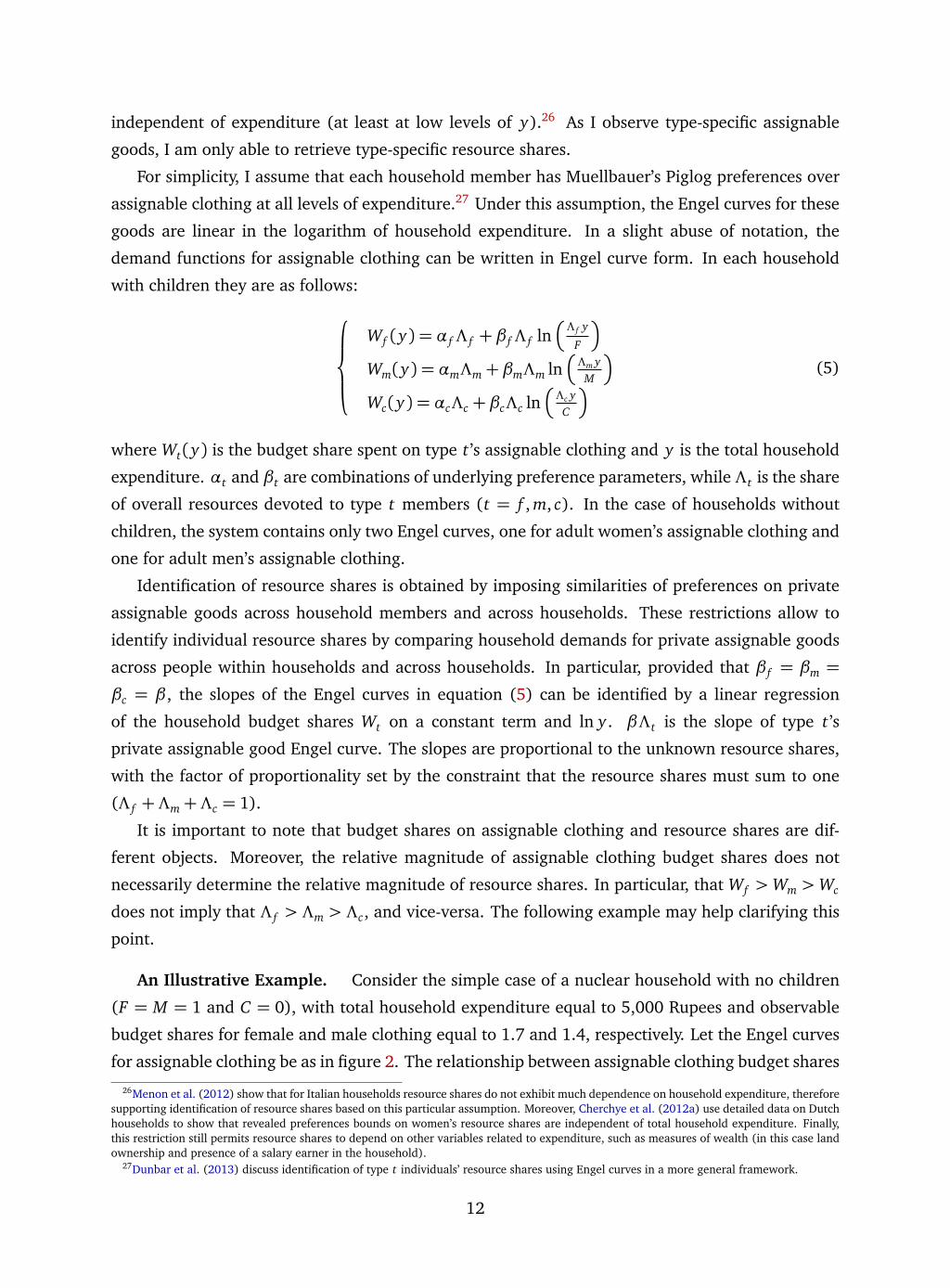
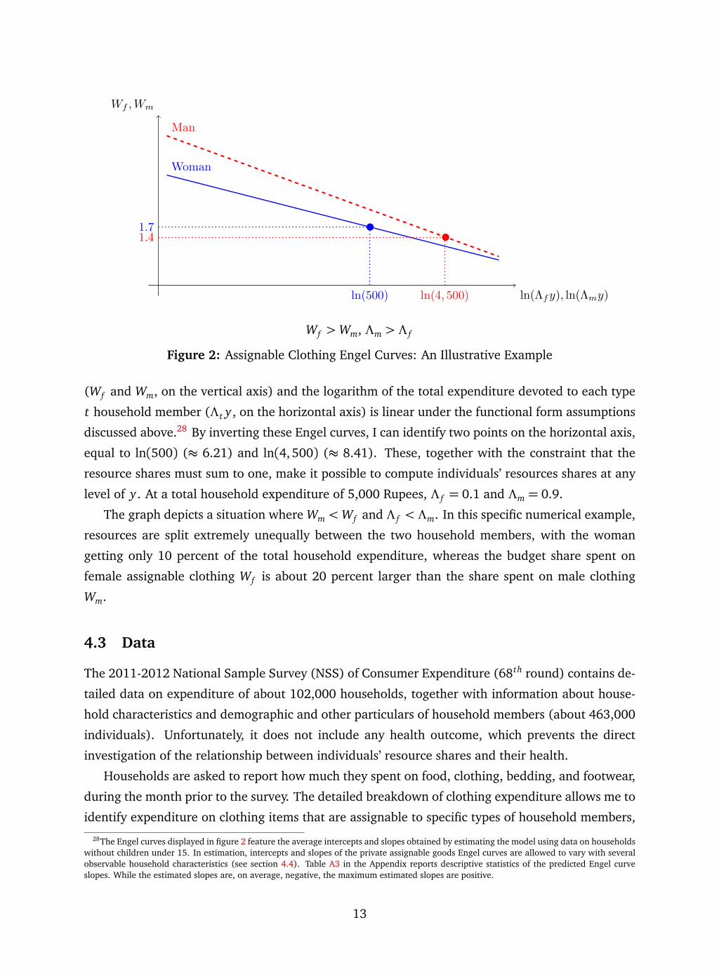
An Illustrative Example. Consider the simple case of a nuclear household with no children

(F = M = 1 and C = 0), with total household expenditure equal to 5,000 Rupees and observable

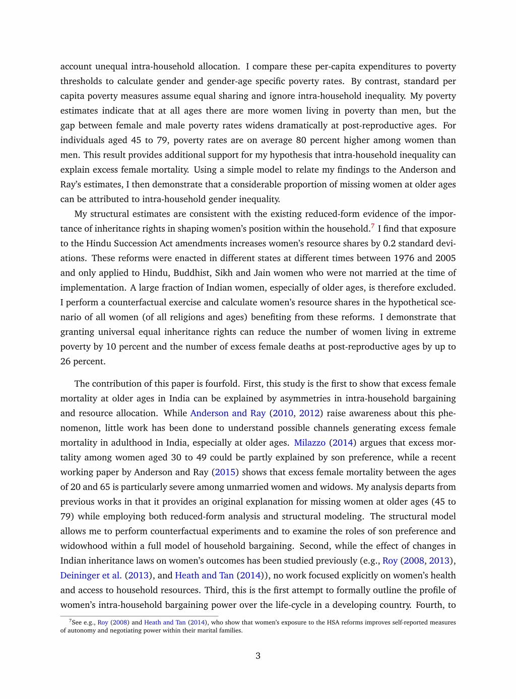
budget shares for female and male clothing equal to 1.7 and 1.4, respectively. Let the Engel curves

for assignable clothing be as in figure 2. The relationship between assignable clothing budget shares

26Menon et al. (2012) show that for Italian households resource shares do not exhibit much dependence on household expenditure, thereforesupporting identification of resource shares based on this particular assumption. Moreover, Cherchye et al. (2012a) use detailed data on Dutchhouseholds to show that revealed preferences bounds on women’s resource shares are independent of total household expenditure. Finally,this restriction still permits resource shares to depend on other variables related to expenditure, such as measures of wealth (in this case landownership and presence of a salary earner in the household).

27Dunbar et al. (2013) discuss identification of type t individuals’ resource shares using Engel curves in a more general framework.

12

ln(Λfy), ln(Λmy)

Wf ,Wm

Woman

Man

1.7

ln(500)

1.4

ln(4, 500)

Wf >Wm, Λm > Λ f

Figure 2: Assignable Clothing Engel Curves: An Illustrative Example

(Wf and Wm, on the vertical axis) and the logarithm of the total expenditure devoted to each type

t household member (Λt y , on the horizontal axis) is linear under the functional form assumptions

discussed above.28 By inverting these Engel curves, I can identify two points on the horizontal axis,

equal to ln(500) (≈ 6.21) and ln(4, 500) (≈ 8.41). These, together with the constraint that the

resource shares must sum to one, make it possible to compute individuals’ resources shares at any

level of y . At a total household expenditure of 5,000 Rupees, Λ f = 0.1 and Λm = 0.9.

The graph depicts a situation where Wm <Wf and Λ f < Λm. In this specific numerical example,

resources are split extremely unequally between the two household members, with the woman

getting only 10 percent of the total household expenditure, whereas the budget share spent on

female assignable clothing Wf is about 20 percent larger than the share spent on male clothing

Wm.

4.3 Data

The 2011-2012 National Sample Survey (NSS) of Consumer Expenditure (68th round) contains de-

tailed data on expenditure of about 102,000 households, together with information about house-

hold characteristics and demographic and other particulars of household members (about 463,000

individuals). Unfortunately, it does not include any health outcome, which prevents the direct

investigation of the relationship between individuals’ resource shares and their health.

Households are asked to report how much they spent on food, clothing, bedding, and footwear,

during the month prior to the survey. The detailed breakdown of clothing expenditure allows me to

identify expenditure on clothing items that are assignable to specific types of household members,

28The Engel curves displayed in figure 2 feature the average intercepts and slopes obtained by estimating the model using data on householdswithout children under 15. In estimation, intercepts and slopes of the private assignable goods Engel curves are allowed to vary with severalobservable household characteristics (see section 4.4). Table A3 in the Appendix reports descriptive statistics of the predicted Engel curveslopes. While the estimated slopes are, on average, negative, the maximum estimated slopes are positive.

13

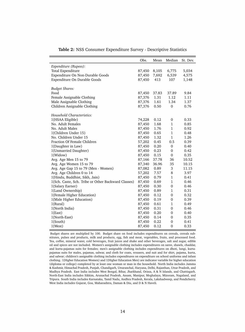
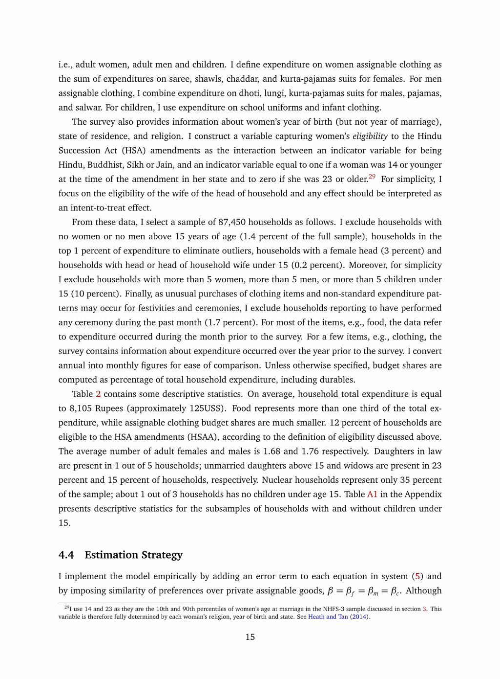
Table 2: NSS Consumer Expenditure Survey - Descriptive Statistics

Obs. Mean Median St. Dev.

Expenditure (Rupees):Total Expenditure 87,450 8,105 6,775 5,034Expenditure On Non-Durable Goods 87,450 7,692 6,539 4,575Expenditure On Durable Goods 87,450 413 107 1,148

Budget Shares:Food 87,450 37.83 37.89 9.84Female Assignable Clothing 87,376 1.31 1.12 1.11Male Assignable Clothing 87,376 1.61 1.34 1.37Children Assignable Clothing 87,376 0.50 0 0.76

Household Characteristics:I(HSAA Eligible) 74,228 0.12 0 0.33No. Adult Females 87,450 1.68 1 0.85No. Adult Males 87,450 1.76 1 0.92I(Children Under 15) 87,450 0.65 1 0.48No. Children Under 15 87,450 1.32 1 1.26Fraction Of Female Children 57,202 0.45 0.5 0.39I(Daughter in Law) 87,450 0.20 0 0.40I(Unmarried Daughter) 87,450 0.23 0 0.42I(Widow) 87,450 0.15 0 0.35Avg. Age Men 15 to 79 87,166 37.78 36 10.52Avg. Age Women 15 to 79 87,340 36.96 35 10.15Avg. Age Gap 15 to 79 (Men - Women) 87,082 0.89 3 11.15Avg. Age Children 0 to 14 57,202 7.57 8 3.97I(Hindu, Buddhist, Sikh, Jain) 87,450 0.79 1 0.41I(Sch. Caste, Sch. Tribe or Other Backward Classes) 87,450 0.69 1 0.46I(Salary Earner) 87,450 0.30 0 0.46I(Land Ownership) 87,450 0.89 1 0.31I(Female Higher Education) 87,450 0.12 0 0.32I(Male Higher Education) 87,450 0.19 0 0.39I(Rural) 87,450 0.61 1 0.49I(North India) 87,450 0.31 0 0.46I(East) 87,450 0.20 0 0.40I(North-East) 87,450 0.14 0 0.35I(South) 87,450 0.22 0 0.41I(West) 87,450 0.12 0 0.33

Budget shares are multiplied by 100. Budget share on food includes expenditures on cereals, cereals sub-stitutes, pulses and products, milk and products, egg, fish and meat, vegetables, fruits, and processed food.Tea, coffee, mineral water, cold beverages, fruit juices and shake and other beverages, salt and sugar, edibleoil and spices are not included. Women’s assignable clothing includes expenditures on saree, shawls, chaddar,and kurta-pajamas suits for females; men’s assignable clothing includes expenditures on dhoti, lungi, kurta-pajamas suits for males, pajamas, salwar, and cloth for coats, trousers, and suit and for shirt, pajama, kurta,and salwar; children’s assignable clothing includes expenditures on expenditure on school uniforms and infantclothing. I(Higher Education Women) and I(Higher Education Men) are indicator variable for higher education(diploma or college) completed by at least one woman or man in the household. North India includes Jammu& Kashmir, Himachal Pradesh, Punjab, Chandigarh, Uttaranchal, Haryana, Delhi, Rajasthan, Uttar Pradesh, andMadhya Pradesh. East India includes West Bengal, Bihar, Jharkhand, Orissa, A & N Islands, and Chattisgarh.North-East India includes Sikkim, Arunachal Pradesh, Assam, Manipur, Meghalaya, Mizoram, Nagaland, andTripura. South India includes Karnataka, Tamil Nadu, Andhra Pradesh, Kerala, Lakshadweep, and Pondicherry.West India includes Gujarat, Goa, Maharashtra, Daman & Diu, and D & N Haveli.

14

i.e., adult women, adult men and children. I define expenditure on women assignable clothing as

the sum of expenditures on saree, shawls, chaddar, and kurta-pajamas suits for females. For men

assignable clothing, I combine expenditure on dhoti, lungi, kurta-pajamas suits for males, pajamas,

and salwar. For children, I use expenditure on school uniforms and infant clothing.

The survey also provides information about women’s year of birth (but not year of marriage),

state of residence, and religion. I construct a variable capturing women’s eligibility to the Hindu

Succession Act (HSA) amendments as the interaction between an indicator variable for being

Hindu, Buddhist, Sikh or Jain, and an indicator variable equal to one if a woman was 14 or younger

at the time of the amendment in her state and to zero if she was 23 or older.29 For simplicity, I

focus on the eligibility of the wife of the head of household and any effect should be interpreted as

an intent-to-treat effect.

From these data, I select a sample of 87,450 households as follows. I exclude households with

no women or no men above 15 years of age (1.4 percent of the full sample), households in the

top 1 percent of expenditure to eliminate outliers, households with a female head (3 percent) and

households with head or head of household wife under 15 (0.2 percent). Moreover, for simplicity

I exclude households with more than 5 women, more than 5 men, or more than 5 children under

15 (10 percent). Finally, as unusual purchases of clothing items and non-standard expenditure pat-

terns may occur for festivities and ceremonies, I exclude households reporting to have performed

any ceremony during the past month (1.7 percent). For most of the items, e.g., food, the data refer

to expenditure occurred during the month prior to the survey. For a few items, e.g., clothing, the

survey contains information about expenditure occurred over the year prior to the survey. I convert

annual into monthly figures for ease of comparison. Unless otherwise specified, budget shares are

computed as percentage of total household expenditure, including durables.

Table 2 contains some descriptive statistics. On average, household total expenditure is equal

to 8,105 Rupees (approximately 125US$). Food represents more than one third of the total ex-

penditure, while assignable clothing budget shares are much smaller. 12 percent of households are

eligible to the HSA amendments (HSAA), according to the definition of eligibility discussed above.

The average number of adult females and males is 1.68 and 1.76 respectively. Daughters in law

are present in 1 out of 5 households; unmarried daughters above 15 and widows are present in 23

percent and 15 percent of households, respectively. Nuclear households represent only 35 percent

of the sample; about 1 out of 3 households has no children under age 15. Table A1 in the Appendix

presents descriptive statistics for the subsamples of households with and without children under

15.

4.4 Estimation Strategy

I implement the model empirically by adding an error term to each equation in system (5) and

by imposing similarity of preferences over private assignable goods, β = β f = βm = βc. Although

29I use 14 and 23 as they are the 10th and 90th percentiles of women’s age at marriage in the NHFS-3 sample discussed in section 3. Thisvariable is therefore fully determined by each woman’s religion, year of birth and state. See Heath and Tan (2014).

15

not required for the identification of the resource shares, I augment the system of Engel curves

of private assignable goods with the inclusion of the household level Engel curve for food. The

inclusion of this extra equation has a double motivation. On one hand, as the error terms are

likely correlated between the equations, it may improve efficiency. On the other hand, it makes

it possible to test whether the food Engel curve is downward sloping in this context.30 Since the

error terms may be correlated across equations, I estimate the system using non-linear Seemingly

Unrelated Regression (SUR) method. Non-linear SUR is iterated until the estimated parameters and

the covariance matrix settle. Iterated SUR is equivalent to maximum likelihood with multivariate

normal errors.

I take the following system of equations to the data:

Wf ood = α f ood + β f ood ln y + ε f ood

Wf = α fΛ f + βΛ f ln�

Λ f

F

�

+ βΛ f ln y + ε f

Wm = αmΛm+ βΛm ln�

Λm

M

�

+ βΛm ln y + εm

Wc = αcΛc + βΛc ln�

Λc

C

�

+ βΛc ln y + εc

(6)

where Λc = 1− Λ f − Λm. y is the total household expenditure (in Rupees) reported for the

month prior to the survey, and Wt and Wf ood are the budget shares spent on assignable clothing

and food, respectively. For households without children under 15, the system includes only the first

three equations and Λm = 1−Λ f .

I account for observable heterogeneity across households by specifying αt (t = f , m, c) and

β as linear functions of observable household characteristics (preference factors, X ). Moreover,

Λt , α f ood and β f ood depend linearly on X and one distribution factor, d.31 This characterization

renders the system of Engel curves non-linear. The vector X = (X1, ..., Xn) includes, among other

variables, details about the composition of the household, socio-economic characteristics, such as

demographic group, religion and land ownership, and polynomials in women’s age and in the age

gap between genders. It also contains region fixed effects (South, East, West, North-East, North,

with West being the excluded category) and a dummy variable for living in rural areas, which

may capture unobserved geographical heterogeneity and area specific characteristics, such as price

levels.32 Although distribution factors are not required for identification, I include eligibility of the

wife of the head of the household to the HSA amendments as a factor affecting resource allocation

but not preferences.33

30This prediction is known as the Engel’s law. Although the underlying preference parameters for food cannot be separately identified, boththe intercept and the slope of the additional equation in the system can.

31Since resource shares cannot be disentangled from preference parameters in the food equation, intercept and slope are allowed to dependon d as well. For each type t = f , m, c and T = F, M , C , total resource shares are specified as Λt = lt,0+ lt,1X1+ ...+ lt,nXn+ l d, where n= 22for households without children, and n = 25 for households with children. The same holds true for α f ood and β f ood . αt , t = f , m, c and β arespecified as linear functions of X where again n= 22 for households without children, and n= 25 for households with children.

32The choice of including the region instead of state fixed effects is due to computational tractability.33Legal reforms have been used in the literature as distribution factors. Chiappori et al. (2002), for example, use US divorce laws as

distribution factors to study intra-household bargaining and labor supply, while Voena (2015) examines how divorce laws affect couples’intertemporal choices in a dynamic model of household decision-making. Despite being permitted by the Indian legislation, there is a strongsocial stigma of divorce in India, which renders it an inadequate distribution factor. As HSA amendments reforms only applied to women whogot married after the implementation, it is sensible to assume that they do not determine shifts in bargaining power over time and that their

16

I estimate models for households with and without children below 15, jointly and separately.

Robust standard errors are clustered at the first sampling unit (2001 Census villages in rural ar-

eas and 2007-2012 Urban Frame Survey blocks in urban areas). Results are robust to clustering

standard errors at the district level.

4.5 Estimation Results

Table 3 reports the estimated coefficients of the covariates (X1, ...Xn, d). I refer to these variables

as the potential determinants of women’s resource share, as they are related to bargaining power,

but not necessarily in a causal sense.34 Column 1 reports the estimation results obtained when all

households are considered in estimation. In columns 2 and 3, I present the results obtained by

estimating separate models for households with and without children under 15.

As expected, households composition matters. Women’s resource shares increase with the num-

ber of women in the household, and decrease with the number of men. Everything else equal, the

presence of an additional woman increases women’s resource shares by 3.9 percentage points in

the overall sample, by 3.3 percentage points in households with children and by 6.2 percentage

points in households without children. While the number of children per se does not seem to play

a significant role, the fraction of female children is positively related to Λ f : if all children are girls,

women’s resource shares are 1.3 percentage points larger. This result is in line with the findings

in Dunbar et al. (2013) and can be attributed to the fact that adult women may be willing (or

required) to forgo a higher fraction of household resources in presence of male children, due to

son preference. Moreover, the presence of a widow in the household is associated with a smaller

resource share for women, especially in households without children, which confirms the previous

work on the plight of widows in South Asia.35 Finally, the higher is women’s age the lower is the

fraction of household’s total expenditure devoted to women, everything else equal.36 This finding

is particularly relevant in households without children, which suggest that women’s bargaining

position inside the household may be tightly related to child rearing.

Household socio-economic characteristics also play an important role. In particular, being part

of Scheduled Caste, Scheduled Tribes, and other disadvantaged social classes is associated with

higher women’s bargaining power. The same holds true for residing in the North-East states, which

is consistent with the presence of a number of matrilineal societies and cultures (Khasi and Garo

societies, for example). In contrast, North Indian women seem to have a much lower bargaining

power. Households with more educated women and men devote a larger fraction of their resources

to women, while the presence of a salary earner (male, in most cases) is associated with lower

women’s bargaining power.37

effects can be analyzed using a static framework.34The estimated coefficients of the covariates for men’s and children’s resource shares and for the preference parameters α f ood , αt , t =

f , m, c, β f ood , and β are available upon request.35See e.g., Drèze et al. (1990), Chen and Drèze (1995), Drèze and Srinivasan (1997), and the recent work by Anderson and Ray (2015) on

missing unmarried women.36Women’s age, children’s age and age differences are divided by 100 for ease of computation.37While male labor force participation is almost universal, only one woman out of three in India does any non-domestic work and an even

17

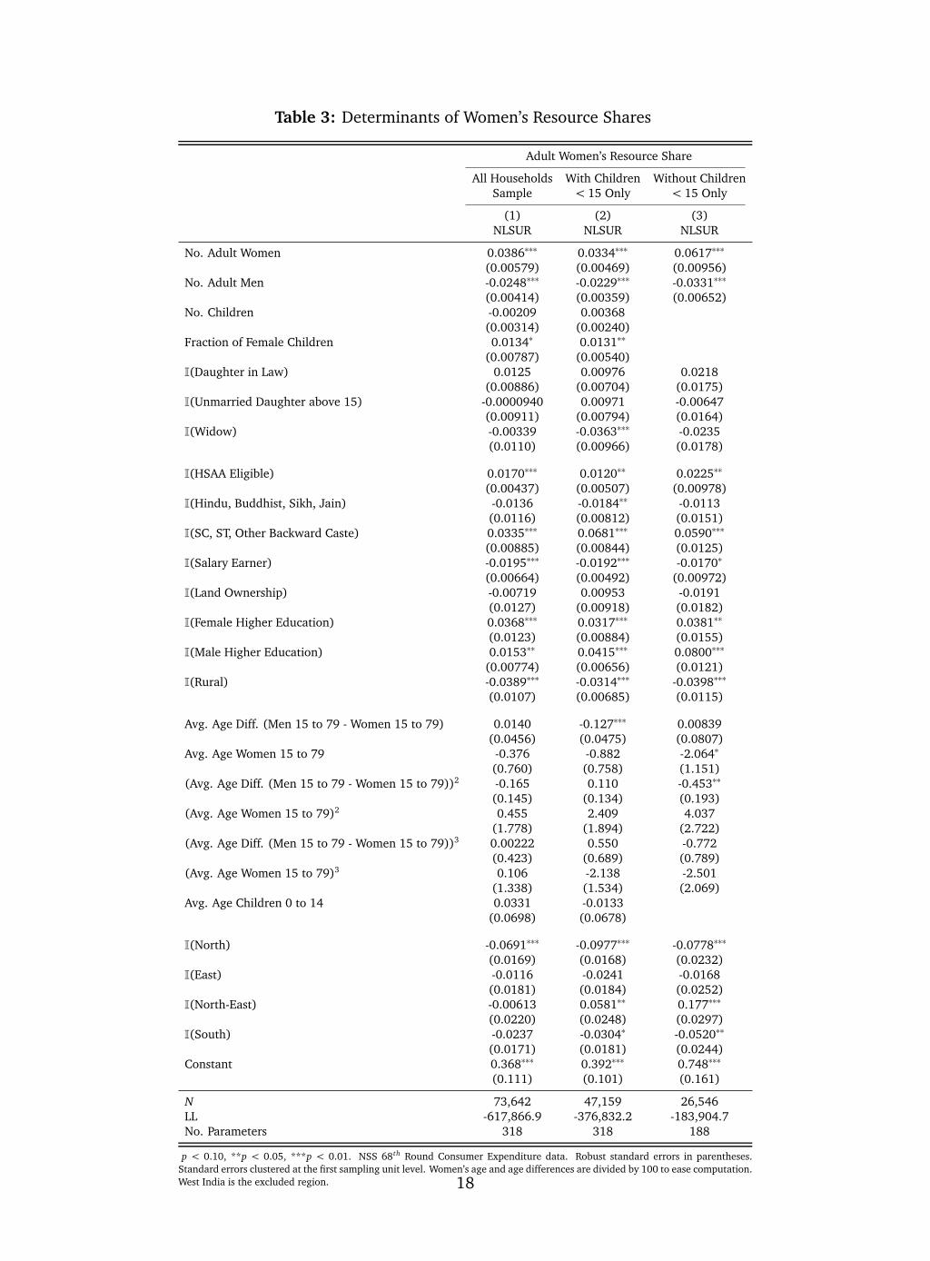
Table 3: Determinants of Women’s Resource Shares

Adult Women’s Resource Share

All Households With Children Without ChildrenSample < 15 Only < 15 Only

(1) (2) (3)NLSUR NLSUR NLSUR

No. Adult Women 0.0386∗∗∗ 0.0334∗∗∗ 0.0617∗∗∗

(0.00579) (0.00469) (0.00956)No. Adult Men -0.0248∗∗∗ -0.0229∗∗∗ -0.0331∗∗∗

(0.00414) (0.00359) (0.00652)No. Children -0.00209 0.00368

(0.00314) (0.00240)Fraction of Female Children 0.0134∗ 0.0131∗∗

(0.00787) (0.00540)I(Daughter in Law) 0.0125 0.00976 0.0218

(0.00886) (0.00704) (0.0175)I(Unmarried Daughter above 15) -0.0000940 0.00971 -0.00647

(0.00911) (0.00794) (0.0164)I(Widow) -0.00339 -0.0363∗∗∗ -0.0235

(0.0110) (0.00966) (0.0178)

I(HSAA Eligible) 0.0170∗∗∗ 0.0120∗∗ 0.0225∗∗

(0.00437) (0.00507) (0.00978)I(Hindu, Buddhist, Sikh, Jain) -0.0136 -0.0184∗∗ -0.0113

(0.0116) (0.00812) (0.0151)I(SC, ST, Other Backward Caste) 0.0335∗∗∗ 0.0681∗∗∗ 0.0590∗∗∗

(0.00885) (0.00844) (0.0125)I(Salary Earner) -0.0195∗∗∗ -0.0192∗∗∗ -0.0170∗

(0.00664) (0.00492) (0.00972)I(Land Ownership) -0.00719 0.00953 -0.0191

(0.0127) (0.00918) (0.0182)I(Female Higher Education) 0.0368∗∗∗ 0.0317∗∗∗ 0.0381∗∗

(0.0123) (0.00884) (0.0155)I(Male Higher Education) 0.0153∗∗ 0.0415∗∗∗ 0.0800∗∗∗

(0.00774) (0.00656) (0.0121)I(Rural) -0.0389∗∗∗ -0.0314∗∗∗ -0.0398∗∗∗

(0.0107) (0.00685) (0.0115)

Avg. Age Diff. (Men 15 to 79 - Women 15 to 79) 0.0140 -0.127∗∗∗ 0.00839(0.0456) (0.0475) (0.0807)

Avg. Age Women 15 to 79 -0.376 -0.882 -2.064∗

(0.760) (0.758) (1.151)(Avg. Age Diff. (Men 15 to 79 - Women 15 to 79))2 -0.165 0.110 -0.453∗∗

(0.145) (0.134) (0.193)(Avg. Age Women 15 to 79)2 0.455 2.409 4.037

(1.778) (1.894) (2.722)(Avg. Age Diff. (Men 15 to 79 - Women 15 to 79))3 0.00222 0.550 -0.772

(0.423) (0.689) (0.789)(Avg. Age Women 15 to 79)3 0.106 -2.138 -2.501

(1.338) (1.534) (2.069)Avg. Age Children 0 to 14 0.0331 -0.0133

(0.0698) (0.0678)

I(North) -0.0691∗∗∗ -0.0977∗∗∗ -0.0778∗∗∗

(0.0169) (0.0168) (0.0232)I(East) -0.0116 -0.0241 -0.0168

(0.0181) (0.0184) (0.0252)I(North-East) -0.00613 0.0581∗∗ 0.177∗∗∗

(0.0220) (0.0248) (0.0297)I(South) -0.0237 -0.0304∗ -0.0520∗∗

(0.0171) (0.0181) (0.0244)Constant 0.368∗∗∗ 0.392∗∗∗ 0.748∗∗∗

(0.111) (0.101) (0.161)

N 73,642 47,159 26,546LL -617,866.9 -376,832.2 -183,904.7No. Parameters 318 318 188

p < 0.10, **p < 0.05, ***p < 0.01. NSS 68th Round Consumer Expenditure data. Robust standard errors in parentheses.Standard errors clustered at the first sampling unit level. Women’s age and age differences are divided by 100 to ease computation.West India is the excluded region. 18

The estimated model confirms the importance of the Hindu Succession Act amendments (HSAA)

in shaping women’s bargaining position within the household. In households where the wife of the

head of household is eligible to these reforms, women’s resource shares are higher by 1.2 to 2.3

percentage points, depending on the model considered for estimation. These results align with the

findings in Roy (2008) and Heath and Tan (2014) on the effects of HSA amendments on women’s

autonomy and bargaining power. Heath and Tan (2014) find that exposure to HSA amendments

is associated with a decrease of 6.6 percentage points in the probability that a woman has no say

in household decisions, an increase of 8.2 percentage points in the probability that a woman can

go to the market alone, a 6.9 percentage point increase in the probability that a woman can go

to a health facility alone, and a 8.3 percentage point increase in the probability that a woman can

travel outside the village alone. As their results rely on self-reported measures of independence

and decision-making power within the household, a direct comparison of the magnitudes is not

straightforward.

I test the hypothesis of equality of coefficients between the models in columns 2 and 3 and find

the likelihood ratio test statistics to be larger than the χ2 critical value. As the null hypothesis

is rejected, in the rest of the paper I focus on the results obtained estimating the two models

separately.

I perform a series of robustness checks to test the sensitivity of the structural estimates. All

results are included in section A.5 of the Appendix. While the findings discussed in this section

are obtained using total expenditure (on durable and non-durable goods), I show that they are

confirmed when estimating the system of Engel curves in terms of expenditure on non-durable

goods only (table A11). Moreover, I estimate the system in (6) without the Engel curve for food,

which follows more closely the analysis in Dunbar et al. (2013), and show that my results hold

(table A12). In addition, I demonstrate that similar conclusions are obtained when estimating the

model using data for households with one individuals for each type (t = f , m, c) only (columns

1 to 3 of table A13), and when estimating a model for married couples with children, where

dummies for the number of children are included as shifters of resource shares and preference

parameters (column 4 of table A13).38 Finally, to check the validity of the theoretical framework, I

use auxiliary data on singles to empirically test the assumption of Pareto efficiency (see section A.6

in the Appendix).

5 Why Are Older Women Missing?

That health and mortality risk are related is indisputable. Section 3 demonstrates that changes in

intra-household bargaining power affect women’s health, therefore validating my hypothesis that

a weak bargaining position can explain excess female mortality. In this section, I argue that older

smaller fraction is formally employed and work for salary (Fulford (2014) and Heath and Tan (2014)).38This specification mirrors that estimated in Dunbar et al. (2013) using data from the Malawi Integrated Household Survey (IHS2). They

look at married couples with up to four children.

19

women are missing in India because their bargaining power diminishes at post-reproductive ages.

First, I use the parameter estimates discussed in the previous section to predict resource shares and

to trace out the age profile of women’s bargaining power and access to household resources. Next,

using these predictions, I compute poverty rates that account for intra-household inequalities and

outline the age distribution of female poverty. Finally, I relate my findings to the age distribution

of missing women estimated by Anderson and Ray (2010) and determine what proportion of these

missing women is attributable to intra-household gender inequality and to the consequent gender

asymmetry in poverty.

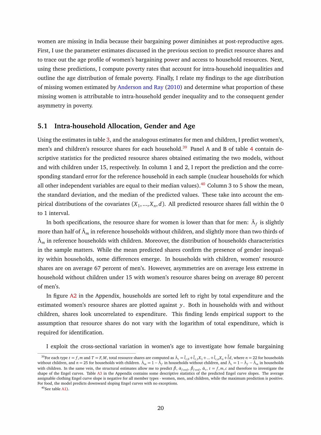
5.1 Intra-household Allocation, Gender and Age

Using the estimates in table 3, and the analogous estimates for men and children, I predict women’s,

men’s and children’s resource shares for each household.39 Panel A and B of table 4 contain de-

scriptive statistics for the predicted resource shares obtained estimating the two models, without

and with children under 15, respectively. In column 1 and 2, I report the prediction and the corre-

sponding standard error for the reference household in each sample (nuclear households for which

all other independent variables are equal to their median values).40 Column 3 to 5 show the mean,

the standard deviation, and the median of the predicted values. These take into account the em-

pirical distributions of the covariates (X1, ..., Xn, d). All predicted resource shares fall within the 0

to 1 interval.

In both specifications, the resource share for women is lower than that for men: Λ f is slightly

more than half of Λm in reference households without children, and slightly more than two thirds of

Λm in reference households with children. Moreover, the distribution of households characteristics

in the sample matters. While the mean predicted shares confirm the presence of gender inequal-

ity within households, some differences emerge. In households with children, women’ resource

shares are on average 67 percent of men’s. However, asymmetries are on average less extreme in

household without children under 15 with women’s resource shares being on average 80 percent

of men’s.

In figure A2 in the Appendix, households are sorted left to right by total expenditure and the

estimated women’s resource shares are plotted against y . Both in households with and without

children, shares look uncorrelated to expenditure. This finding lends empirical support to the

assumption that resource shares do not vary with the logarithm of total expenditure, which is

required for identification.

I exploit the cross-sectional variation in women’s age to investigate how female bargaining

39For each type t = f , m and T = F, M , total resource shares are computed as Λt = lt,0+ lt,1X1+ ...+ lt,nXn+ˆld, where n= 22 for households

without children, and n= 25 for households with children. Λm = 1− Λ f in households without children, and Λc = 1− Λ f − Λm in householdswith children. In the same vein, the structural estimates allow me to predict β , α f ood , β f ood , αt , t = f , m, c and therefore to investigate theshape of the Engel curves. Table A3 in the Appendix contains some descriptive statistics of the predicted Engel curve slopes. The averageassignable clothing Engel curve slope is negative for all member types - women, men, and children, while the maximum prediction is positive.For food, the model predicts downward sloping Engel curves with no exceptions.

40See table A1).

20

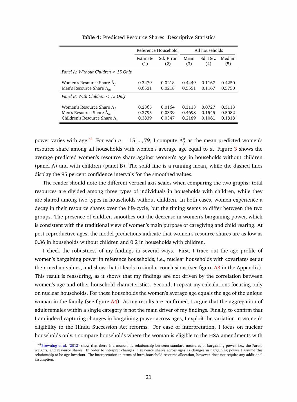
Table 4: Predicted Resource Shares: Descriptive Statistics

Reference Household All households

Estimate Sd. Error Mean Sd. Dev. Median(1) (2) (3) (4) (5)

Panel A: Without Children < 15 Only

Women’s Resource Share Λ f 0.3479 0.0218 0.4449 0.1167 0.4250Men’s Resource Share Λm 0.6521 0.0218 0.5551 0.1167 0.5750

Panel B: With Children < 15 Only

Women’s Resource Share Λ f 0.2365 0.0164 0.3113 0.0727 0.3113Men’s Resource Share Λm 0.3795 0.0339 0.4698 0.1545 0.5082Children’s Resource Share Λc 0.3839 0.0347 0.2189 0.1061 0.1818

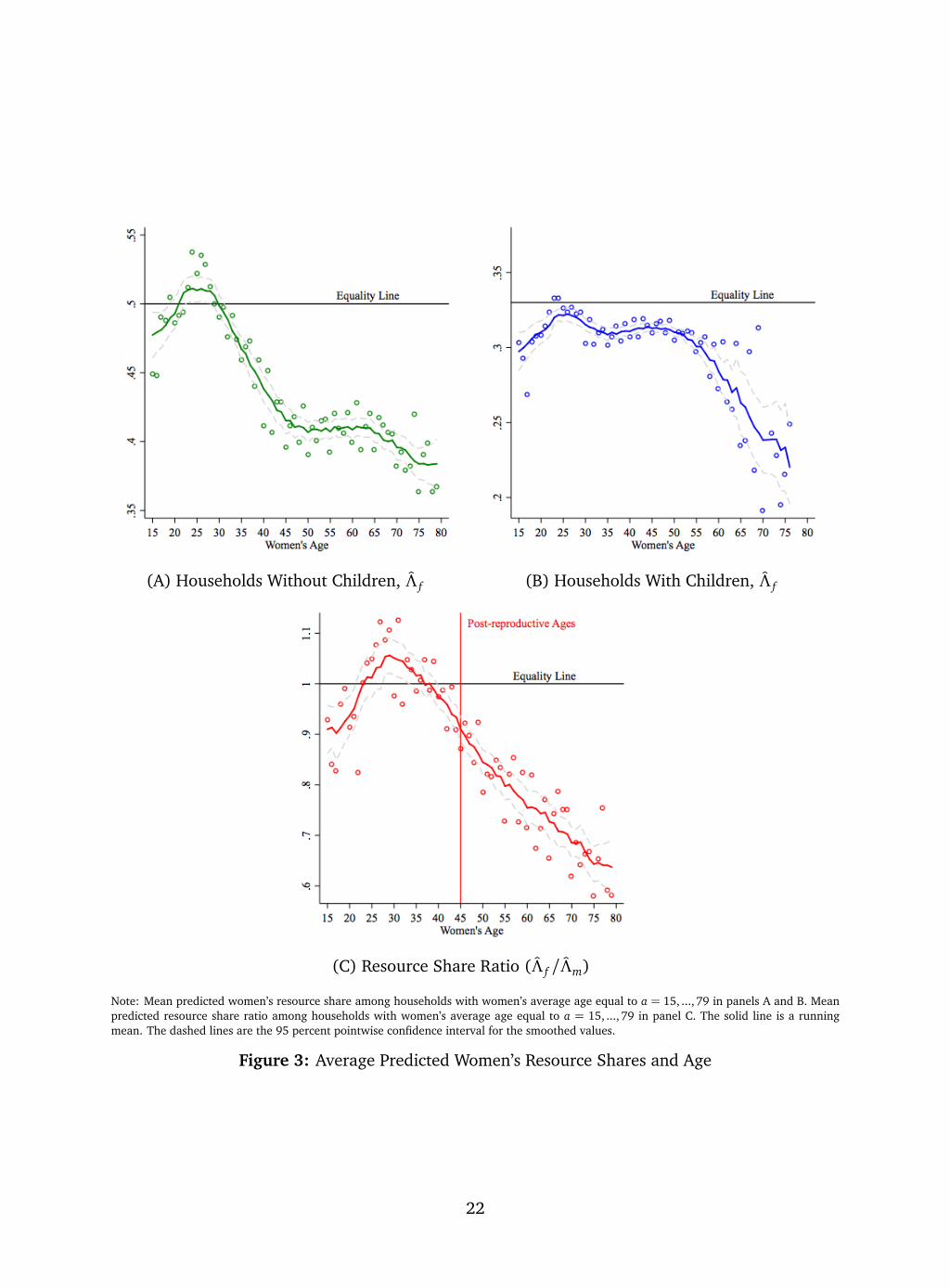
power varies with age.41 For each a = 15, ..., 79, I compute Λaf as the mean predicted women’s

resource share among all households with women’s average age equal to a. Figure 3 shows the

average predicted women’s resource share against women’s age in households without children

(panel A) and with children (panel B). The solid line is a running mean, while the dashed lines

display the 95 percent confidence intervals for the smoothed values.

The reader should note the different vertical axis scales when comparing the two graphs: total

resources are divided among three types of individuals in households with children, while they

are shared among two types in households without children. In both cases, women experience a

decay in their resource shares over the life-cycle, but the timing seems to differ between the two

groups. The presence of children smoothes out the decrease in women’s bargaining power, which

is consistent with the traditional view of women’s main purpose of caregiving and child rearing. At

post-reproductive ages, the model predictions indicate that women’s resource shares are as low as

0.36 in households without children and 0.2 in households with children.

I check the robustness of my findings in several ways. First, I trace out the age profile of

women’s bargaining power in reference households, i.e., nuclear households with covariates set at

their median values, and show that it leads to similar conclusions (see figure A3 in the Appendix).

This result is reassuring, as it shows that my findings are not driven by the correlation between

women’s age and other household characteristics. Second, I repeat my calculations focusing only

on nuclear households. For these households the women’s average age equals the age of the unique

woman in the family (see figure A4). As my results are confirmed, I argue that the aggregation of

adult females within a single category is not the main driver of my findings. Finally, to confirm that

I am indeed capturing changes in bargaining power across ages, I exploit the variation in women’s

eligibility to the Hindu Succession Act reforms. For ease of interpretation, I focus on nuclear

households only. I compare households where the woman is eligible to the HSA amendments with

41Browning et al. (2013) show that there is a monotonic relationship between standard measures of bargaining power, i.e., the Paretoweights, and resource shares. In order to interpret changes in resource shares across ages as changes in bargaining power I assume thisrelationship to be age invariant. The interpretation in terms of intra-household resource allocation, however, does not require any additionalassumption.

21

(A) Households Without Children, Λ f (B) Households With Children, Λ f

(C) Resource Share Ratio (Λ f /Λm)

Note: Mean predicted women’s resource share among households with women’s average age equal to a = 15, ..., 79 in panels A and B. Meanpredicted resource share ratio among households with women’s average age equal to a = 15, ..., 79 in panel C. The solid line is a runningmean. The dashed lines are the 95 percent pointwise confidence interval for the smoothed values.

Figure 3: Average Predicted Women’s Resource Shares and Age

22

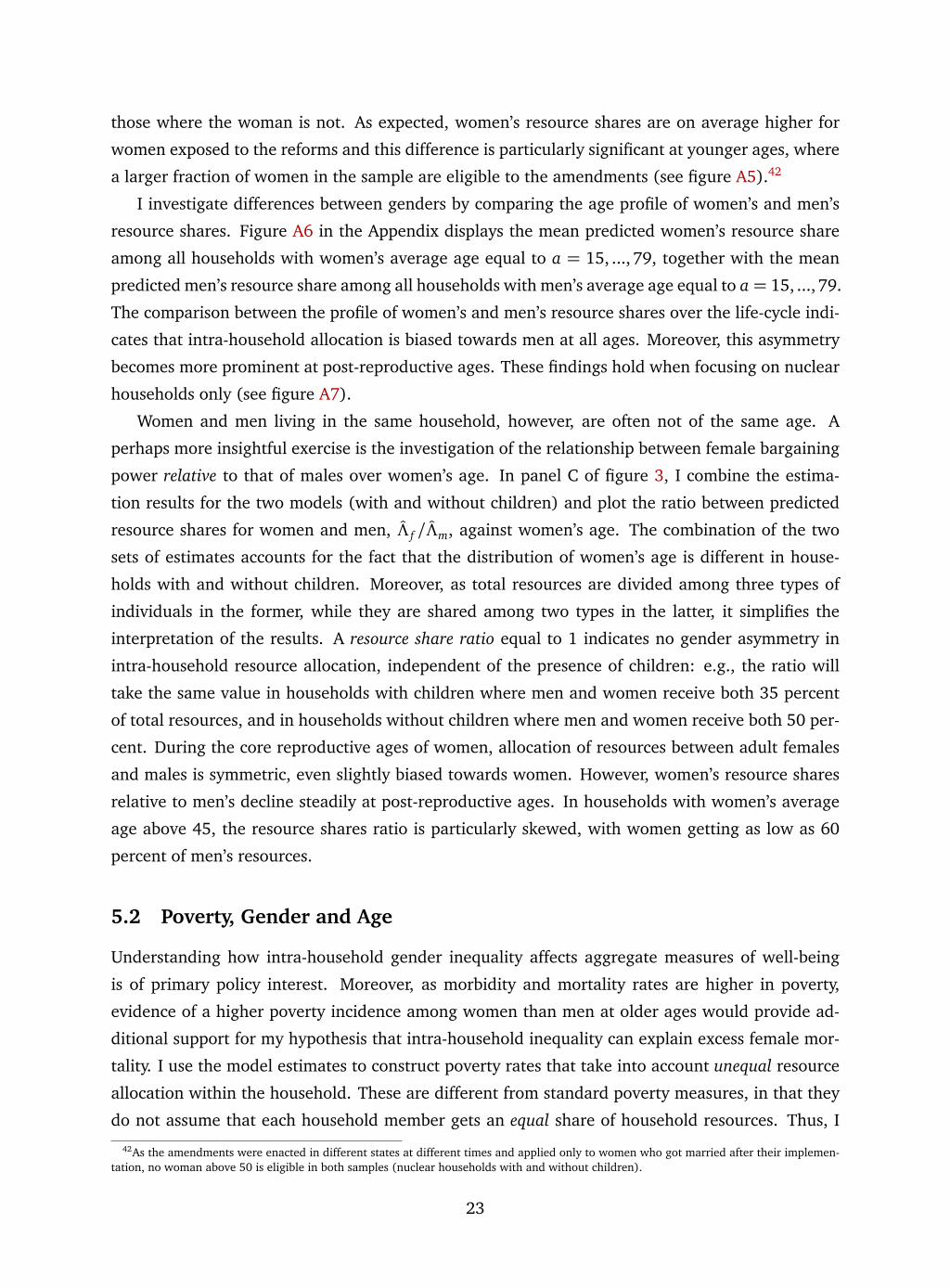
those where the woman is not. As expected, women’s resource shares are on average higher for

women exposed to the reforms and this difference is particularly significant at younger ages, where

a larger fraction of women in the sample are eligible to the amendments (see figure A5).42

I investigate differences between genders by comparing the age profile of women’s and men’s

resource shares. Figure A6 in the Appendix displays the mean predicted women’s resource share

among all households with women’s average age equal to a = 15, ..., 79, together with the mean

predicted men’s resource share among all households with men’s average age equal to a = 15, ..., 79.

The comparison between the profile of women’s and men’s resource shares over the life-cycle indi-

cates that intra-household allocation is biased towards men at all ages. Moreover, this asymmetry

becomes more prominent at post-reproductive ages. These findings hold when focusing on nuclear

households only (see figure A7).

Women and men living in the same household, however, are often not of the same age. A

perhaps more insightful exercise is the investigation of the relationship between female bargaining

power relative to that of males over women’s age. In panel C of figure 3, I combine the estima-

tion results for the two models (with and without children) and plot the ratio between predicted

resource shares for women and men, Λ f /Λm, against women’s age. The combination of the two

sets of estimates accounts for the fact that the distribution of women’s age is different in house-

holds with and without children. Moreover, as total resources are divided among three types of

individuals in the former, while they are shared among two types in the latter, it simplifies the

interpretation of the results. A resource share ratio equal to 1 indicates no gender asymmetry in

intra-household resource allocation, independent of the presence of children: e.g., the ratio will

take the same value in households with children where men and women receive both 35 percent

of total resources, and in households without children where men and women receive both 50 per-

cent. During the core reproductive ages of women, allocation of resources between adult females

and males is symmetric, even slightly biased towards women. However, women’s resource shares

relative to men’s decline steadily at post-reproductive ages. In households with women’s average

age above 45, the resource shares ratio is particularly skewed, with women getting as low as 60

percent of men’s resources.

5.2 Poverty, Gender and Age

Understanding how intra-household gender inequality affects aggregate measures of well-being

is of primary policy interest. Moreover, as morbidity and mortality rates are higher in poverty,

evidence of a higher poverty incidence among women than men at older ages would provide ad-

ditional support for my hypothesis that intra-household inequality can explain excess female mor-

tality. I use the model estimates to construct poverty rates that take into account unequal resource

allocation within the household. These are different from standard poverty measures, in that they

do not assume that each household member gets an equal share of household resources. Thus, I

42As the amendments were enacted in different states at different times and applied only to women who got married after their implemen-tation, no woman above 50 is eligible in both samples (nuclear households with and without children).

23

Table 5: Poverty Head Count Ratios

Model Predictions (Unequal Sharing) Equal Sharing

Women Men Children Poverty AllSex Ratio

(1) (2) (3) (4) (5)

Panel A: Household Level Poverty Rates

1.25 US$/day 0.1657 0.1177 0.2822 1.4078 0.12802 US$/day 0.4313 0.2759 0.5058 1.5632 0.4250

Panel B: Individual Level Poverty Rates

1.25 US$/day 0.2098 0.1463 0.3925 1.4340 0.15402 US$/day 0.4965 0.3422 0.6231 1.4509 0.4784

allow for the presence, within each household, of individuals who live in poverty and of individuals

who do not.

I compute person level expenditures as the product between total household expenditure and

the individual resource shares, as predicted by the model: λt y = Λt yT

(t = f , m, c, T = F, M , C). I

then construct poverty head count ratios by comparing person level expenditures to poverty lines.

I consider the thresholds set by the World Bank for extreme poverty (1.25 US$/day) and average

poverty (2 US$/day).43 As in Dunbar et al. (2013), I set the poverty lines for children to 60 percent

of adults’, in order to take into account the fact that children may have lower needs, while I use the

same poverty lines for men and women. In section A.7 of the Appendix I investigated deviations

from this last assumption.

By definition, the ratio of female to male poverty rates provides a measure of female poverty

relative to that of males. I call this measure the poverty sex ratio. While a ratio equal to 1 indicates

no gender asymmetry in poverty, a ratio larger than 1 indicates that female poverty is higher than

that of males, and can therefore be interpreted as excess female poverty.

Table 5 reports the poverty estimates. Panel A shows the fraction of households in the sam-

ple living in poverty. Column 1 to 3 report the proportions of households with women, men, or

children living below poverty line, when the model predictions are used to compute person level

expenditures. Column 4 shows the implied poverty sex ratio as defined above. Column 5 reports

the poverty rates obtained under the assumption that each household member gets an equal share

of household resources. In panel B, I present the poverty rates estimated at the individual level,

i.e., the fraction of all individuals, or women, men and children, separately, who live in poverty.

This distinction is quite crucial, as poor and non poor households may have systematically different

size and composition.44

The poverty estimates indicate that there are more households with women living below poverty

43The poverty rate at US$1.25 (US$2) is the proportion of the sample population living on less than US$1.25 (US$2) per day, adjusted forpurchasing power parity (PPP).

44The poverty head counts in the estimation sample are lower than the latest World Bank estimates (2011), which indicate that 24 and59 percent of individuals live below the 1.25 US$/day and 2 US$/day poverty lines at 2005 international prices, respectively. This is notsurprising since a selected sample is used in estimation. See section 4.3 for more details.

24

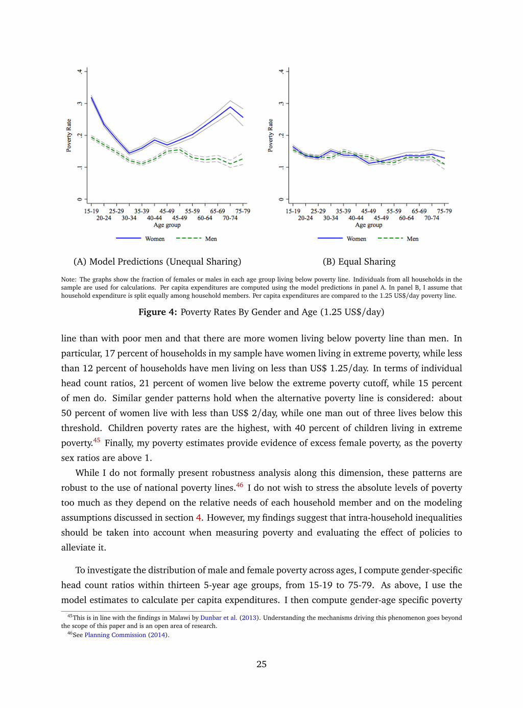
(A) Model Predictions (Unequal Sharing) (B) Equal Sharing

Note: The graphs show the fraction of females or males in each age group living below poverty line. Individuals from all households in thesample are used for calculations. Per capita expenditures are computed using the model predictions in panel A. In panel B, I assume thathousehold expenditure is split equally among household members. Per capita expenditures are compared to the 1.25 US$/day poverty line.

Figure 4: Poverty Rates By Gender and Age (1.25 US$/day)

line than with poor men and that there are more women living below poverty line than men. In

particular, 17 percent of households in my sample have women living in extreme poverty, while less

than 12 percent of households have men living on less than US$ 1.25/day. In terms of individual

head count ratios, 21 percent of women live below the extreme poverty cutoff, while 15 percent

of men do. Similar gender patterns hold when the alternative poverty line is considered: about

50 percent of women live with less than US$ 2/day, while one man out of three lives below this

threshold. Children poverty rates are the highest, with 40 percent of children living in extreme

poverty.45 Finally, my poverty estimates provide evidence of excess female poverty, as the poverty

sex ratios are above 1.

While I do not formally present robustness analysis along this dimension, these patterns are

robust to the use of national poverty lines.46 I do not wish to stress the absolute levels of poverty

too much as they depend on the relative needs of each household member and on the modeling

assumptions discussed in section 4. However, my findings suggest that intra-household inequalities

should be taken into account when measuring poverty and evaluating the effect of policies to

alleviate it.

To investigate the distribution of male and female poverty across ages, I compute gender-specific

head count ratios within thirteen 5-year age groups, from 15-19 to 75-79. As above, I use the

model estimates to calculate per capita expenditures. I then compute gender-age specific poverty

45This is in line with the findings in Malawi by Dunbar et al. (2013). Understanding the mechanisms driving this phenomenon goes beyondthe scope of this paper and is an open area of research.

46See Planning Commission (2014).

25

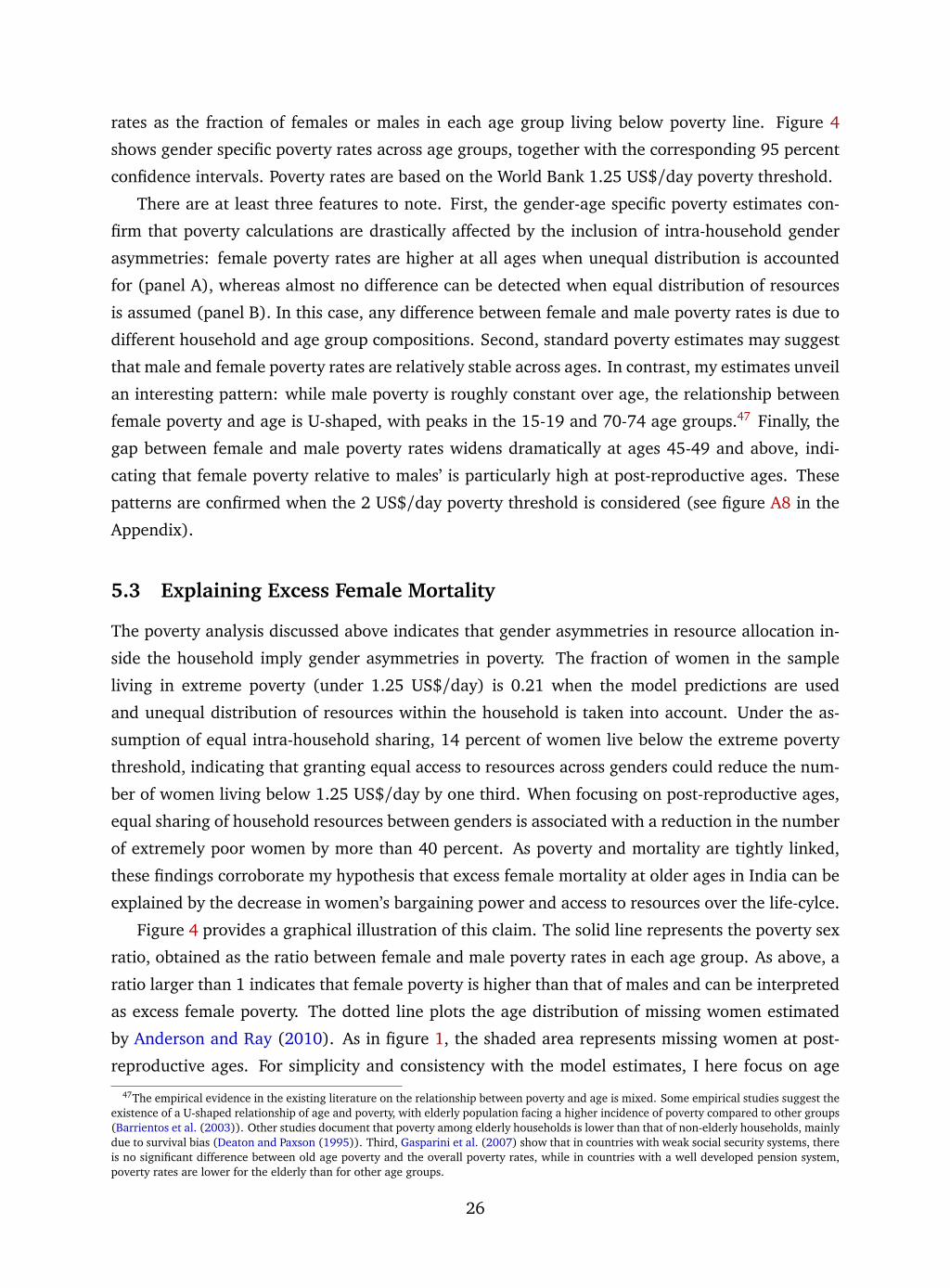
rates as the fraction of females or males in each age group living below poverty line. Figure 4

shows gender specific poverty rates across age groups, together with the corresponding 95 percent

confidence intervals. Poverty rates are based on the World Bank 1.25 US$/day poverty threshold.

There are at least three features to note. First, the gender-age specific poverty estimates con-

firm that poverty calculations are drastically affected by the inclusion of intra-household gender

asymmetries: female poverty rates are higher at all ages when unequal distribution is accounted

for (panel A), whereas almost no difference can be detected when equal distribution of resources

is assumed (panel B). In this case, any difference between female and male poverty rates is due to

different household and age group compositions. Second, standard poverty estimates may suggest

that male and female poverty rates are relatively stable across ages. In contrast, my estimates unveil

an interesting pattern: while male poverty is roughly constant over age, the relationship between

female poverty and age is U-shaped, with peaks in the 15-19 and 70-74 age groups.47 Finally, the

gap between female and male poverty rates widens dramatically at ages 45-49 and above, indi-

cating that female poverty relative to males’ is particularly high at post-reproductive ages. These

patterns are confirmed when the 2 US$/day poverty threshold is considered (see figure A8 in the

Appendix).

5.3 Explaining Excess Female Mortality

The poverty analysis discussed above indicates that gender asymmetries in resource allocation in-

side the household imply gender asymmetries in poverty. The fraction of women in the sample

living in extreme poverty (under 1.25 US$/day) is 0.21 when the model predictions are used

and unequal distribution of resources within the household is taken into account. Under the as-

sumption of equal intra-household sharing, 14 percent of women live below the extreme poverty

threshold, indicating that granting equal access to resources across genders could reduce the num-

ber of women living below 1.25 US$/day by one third. When focusing on post-reproductive ages,

equal sharing of household resources between genders is associated with a reduction in the number

of extremely poor women by more than 40 percent. As poverty and mortality are tightly linked,

these findings corroborate my hypothesis that excess female mortality at older ages in India can be

explained by the decrease in women’s bargaining power and access to resources over the life-cylce.

Figure 4 provides a graphical illustration of this claim. The solid line represents the poverty sex

ratio, obtained as the ratio between female and male poverty rates in each age group. As above, a

ratio larger than 1 indicates that female poverty is higher than that of males and can be interpreted

as excess female poverty. The dotted line plots the age distribution of missing women estimated

by Anderson and Ray (2010). As in figure 1, the shaded area represents missing women at post-

reproductive ages. For simplicity and consistency with the model estimates, I here focus on age

47The empirical evidence in the existing literature on the relationship between poverty and age is mixed. Some empirical studies suggest theexistence of a U-shaped relationship of age and poverty, with elderly population facing a higher incidence of poverty compared to other groups(Barrientos et al. (2003)). Other studies document that poverty among elderly households is lower than that of non-elderly households, mainlydue to survival bias (Deaton and Paxson (1995)). Third, Gasparini et al. (2007) show that in countries with weak social security systems, thereis no significant difference between old age poverty and the overall poverty rates, while in countries with a well developed pension system,poverty rates are lower for the elderly than for other age groups.

26

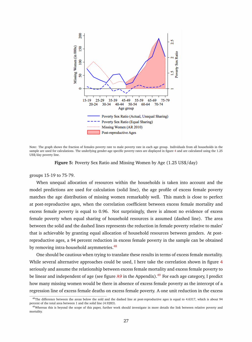
Note: The graph shows the fraction of females poverty rate to male poverty rate in each age group. Individuals from all households in thesample are used for calculations. The underlying gender-age specific poverty rates are displayed in figure 4 and are calculated using the 1.25US$/day poverty line.

Figure 5: Poverty Sex Ratio and Missing Women by Age (1.25 US$/day)

groups 15-19 to 75-79.

When unequal allocation of resources within the households is taken into account and the

model predictions are used for calculation (solid line), the age profile of excess female poverty

matches the age distribution of missing women remarkably well. This match is close to perfect

at post-reproductive ages, when the correlation coefficient between excess female mortality and

excess female poverty is equal to 0.96. Not surprisingly, there is almost no evidence of excess

female poverty when equal sharing of household resources is assumed (dashed line). The area

between the solid and the dashed lines represents the reduction in female poverty relative to males’

that is achievable by granting equal allocation of household resources between genders. At post-

reproductive ages, a 94 percent reduction in excess female poverty in the sample can be obtained

by removing intra-household asymmetries.48

One should be cautious when trying to translate these results in terms of excess female mortality.

While several alternative approaches could be used, I here take the correlation shown in figure 4

seriously and assume the relationship between excess female mortality and excess female poverty to

be linear and independent of age (see figure A9 in the Appendix).49 For each age category, I predict

how many missing women would be there in absence of excess female poverty as the intercept of a

regression line of excess female deaths on excess female poverty. A one unit reduction in the excess

48The difference between the areas below the sold and the dashed line at post-reproductive ages is equal to 4.6317, which is about 94percent of the total area between 1 and the solid line (4.9283).

49Whereas this is beyond the scope of this paper, further work should investigate in more details the link between relative poverty andmortality.

27

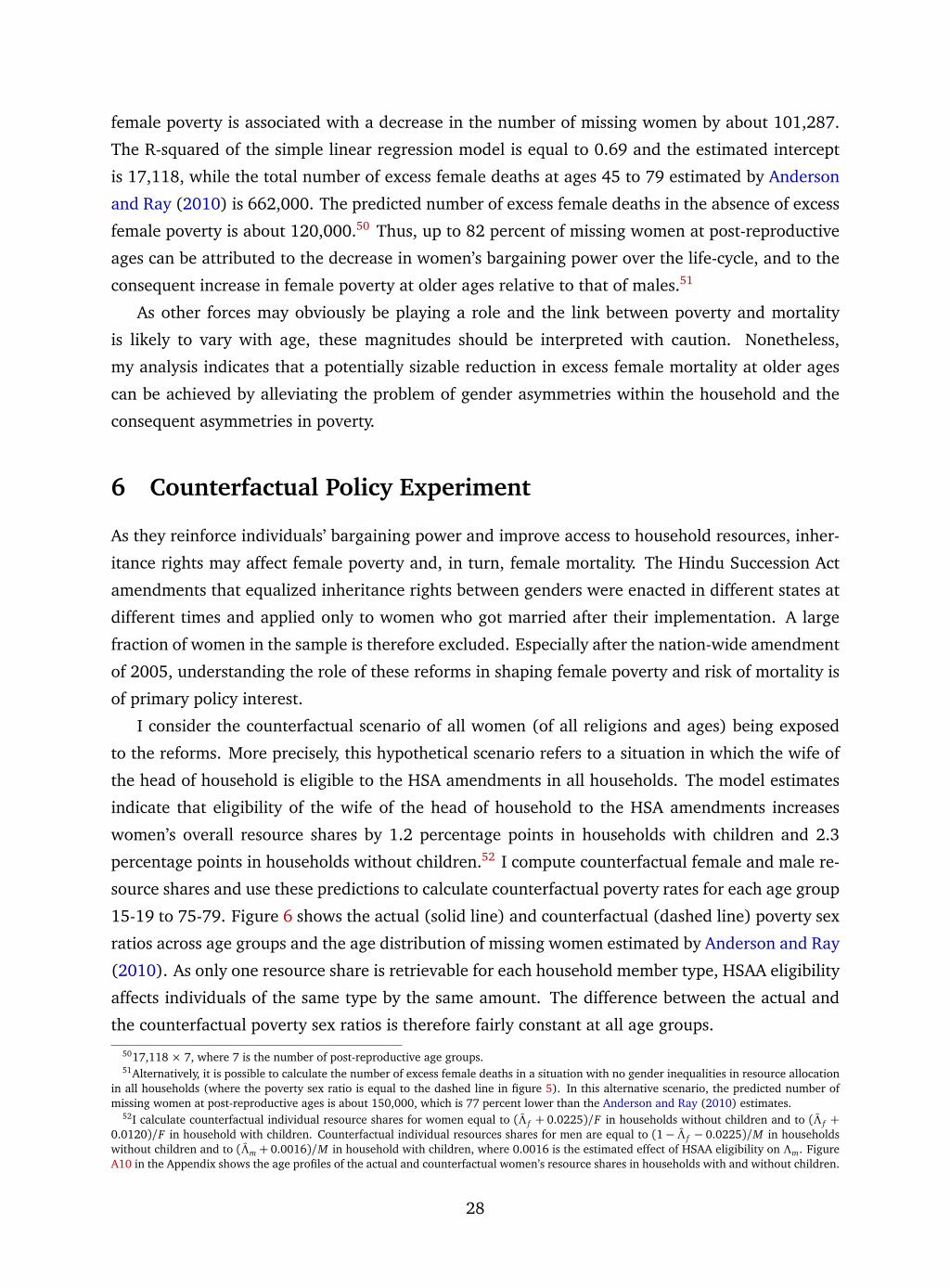
female poverty is associated with a decrease in the number of missing women by about 101,287.

The R-squared of the simple linear regression model is equal to 0.69 and the estimated intercept

is 17,118, while the total number of excess female deaths at ages 45 to 79 estimated by Anderson

and Ray (2010) is 662,000. The predicted number of excess female deaths in the absence of excess

female poverty is about 120,000.50 Thus, up to 82 percent of missing women at post-reproductive

ages can be attributed to the decrease in women’s bargaining power over the life-cycle, and to the

consequent increase in female poverty at older ages relative to that of males.51

As other forces may obviously be playing a role and the link between poverty and mortality

is likely to vary with age, these magnitudes should be interpreted with caution. Nonetheless,

my analysis indicates that a potentially sizable reduction in excess female mortality at older ages

can be achieved by alleviating the problem of gender asymmetries within the household and the

consequent asymmetries in poverty.

6 Counterfactual Policy Experiment

As they reinforce individuals’ bargaining power and improve access to household resources, inher-

itance rights may affect female poverty and, in turn, female mortality. The Hindu Succession Act

amendments that equalized inheritance rights between genders were enacted in different states at

different times and applied only to women who got married after their implementation. A large

fraction of women in the sample is therefore excluded. Especially after the nation-wide amendment

of 2005, understanding the role of these reforms in shaping female poverty and risk of mortality is

of primary policy interest.

I consider the counterfactual scenario of all women (of all religions and ages) being exposed

to the reforms. More precisely, this hypothetical scenario refers to a situation in which the wife of

the head of household is eligible to the HSA amendments in all households. The model estimates

indicate that eligibility of the wife of the head of household to the HSA amendments increases

women’s overall resource shares by 1.2 percentage points in households with children and 2.3

percentage points in households without children.52 I compute counterfactual female and male re-

source shares and use these predictions to calculate counterfactual poverty rates for each age group

15-19 to 75-79. Figure 6 shows the actual (solid line) and counterfactual (dashed line) poverty sex

ratios across age groups and the age distribution of missing women estimated by Anderson and Ray

(2010). As only one resource share is retrievable for each household member type, HSAA eligibility

affects individuals of the same type by the same amount. The difference between the actual and

the counterfactual poverty sex ratios is therefore fairly constant at all age groups.

5017,118 × 7, where 7 is the number of post-reproductive age groups.51Alternatively, it is possible to calculate the number of excess female deaths in a situation with no gender inequalities in resource allocation

in all households (where the poverty sex ratio is equal to the dashed line in figure 5). In this alternative scenario, the predicted number ofmissing women at post-reproductive ages is about 150,000, which is 77 percent lower than the Anderson and Ray (2010) estimates.

52I calculate counterfactual individual resource shares for women equal to (Λ f + 0.0225)/F in households without children and to (Λ f +0.0120)/F in household with children. Counterfactual individual resources shares for men are equal to (1− Λ f − 0.0225)/M in householdswithout children and to (Λm + 0.0016)/M in household with children, where 0.0016 is the estimated effect of HSAA eligibility on Λm. FigureA10 in the Appendix shows the age profiles of the actual and counterfactual women’s resource shares in households with and without children.

28

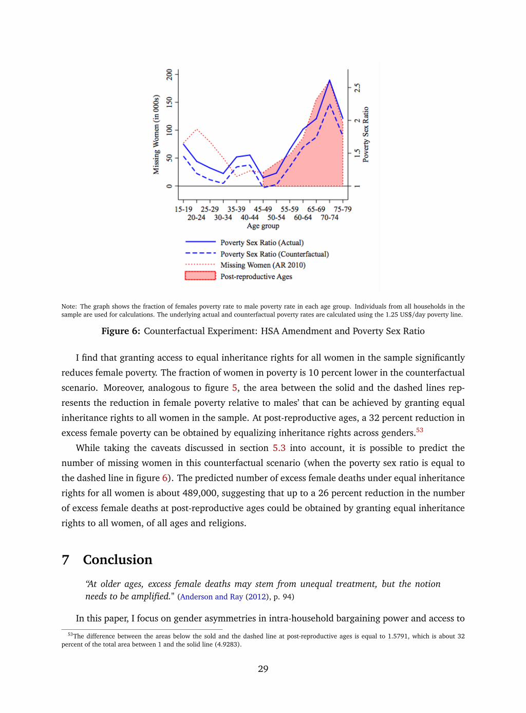
Note: The graph shows the fraction of females poverty rate to male poverty rate in each age group. Individuals from all households in thesample are used for calculations. The underlying actual and counterfactual poverty rates are calculated using the 1.25 US$/day poverty line.

Figure 6: Counterfactual Experiment: HSA Amendment and Poverty Sex Ratio

I find that granting access to equal inheritance rights for all women in the sample significantly

reduces female poverty. The fraction of women in poverty is 10 percent lower in the counterfactual

scenario. Moreover, analogous to figure 5, the area between the solid and the dashed lines rep-

resents the reduction in female poverty relative to males’ that can be achieved by granting equal

inheritance rights to all women in the sample. At post-reproductive ages, a 32 percent reduction in

excess female poverty can be obtained by equalizing inheritance rights across genders.53

While taking the caveats discussed in section 5.3 into account, it is possible to predict the

number of missing women in this counterfactual scenario (when the poverty sex ratio is equal to

the dashed line in figure 6). The predicted number of excess female deaths under equal inheritance

rights for all women is about 489,000, suggesting that up to a 26 percent reduction in the number

of excess female deaths at post-reproductive ages could be obtained by granting equal inheritance

rights to all women, of all ages and religions.

7 Conclusion

“At older ages, excess female deaths may stem from unequal treatment, but the notionneeds to be amplified." (Anderson and Ray (2012), p. 94)

In this paper, I focus on gender asymmetries in intra-household bargaining power and access to

53The difference between the areas below the sold and the dashed line at post-reproductive ages is equal to 1.5791, which is about 32percent of the total area between 1 and the solid line (4.9283).

29

household resources as one form of unequal treatment. I show that a large portion of the missing

women at post-reproductive ages estimated by Anderson and Ray (2010) can be explained by

inequalities in intra-household resource allocation and by the consequent gender asymmetries in

poverty.

The emphasis on intra-household allocation is motivated by the existence of a positive causal

link between women’s bargaining power and their health. I demonstrate this fact by analyzing the

effect of amendments in the Indian inheritance legislation on a set of women’s health outcomes.

These reforms equalized inheritance rights between genders and therefore represent a source of

exogenous variation in women’s position inside the household.

I then provide a structural model for estimating women’s bargaining power, defined as the

fraction of total household expenditure that is consumed by women, and for analyzing its determi-

nants. The model predictions indicate that the allocation of resources between women and men is

symmetric during women’s core reproductive ages, while the share of household resources devoted

to women declines significantly at post-reproductive ages. One consequence of this fact is that at

older ages poverty rates are significantly higher among women than among men. Standard per

capita poverty measures, which by construction ignore intra-household inequality, are unable to

unveil this pattern.

As I demonstrate with my reduced-form analysis and counterfactual experiments, policies aimed

at promoting equality within households, such as improving inheritance rights for women, can

have a large impact on female health, poverty and, in turn, risk of mortality. Future research

should focus on identifying alternative mechanisms generating excess female mortality at post-

reproductive ages and on evaluating policies to successfully tackle the problem of excess female

poverty, especially among the elderly. Moreover, subsequent work should investigate the effects

of the HSA amendments on marital sorting and partner matching. As standard practice in the

collective literature, I take the match as given, but interesting insight might arise from relaxing this

assumption. Finally, in the spirit of Mazzocco (2007), Mazzocco et al. (2014), and Voena (2015),

a promising avenue of research is the investigation of the age profile of women’s bargaining power

using an inter-temporal model in which household members cannot commit to the future allocation

of resources.

References

AGARWAL, B. (1995): “A Field of One’s Own,” Cambridge Books. [7]

ANDERSON, S. AND G. GENICOT (2015): “Suicide and Property Rights in India,” Journal of Develop-ment Economics, 114, 64 – 78. [5]

ANDERSON, S. AND D. RAY (2010): “Missing Women: Age and Disease,” Review of Economic Studies,77, 1262–1300. [1], [3], [5], [20], [26], [28], [30], [36]

——— (2012): “The Age Distribution of Missing Women in India,” Economic and Political Weekly,47, 87–95. [1], [3], [5], [29]

30

——— (2015): “Missing Unmarried Women,” Working Paper 21511, National Bureau of EconomicResearch. [3], [5], [17]

ANUKRITI, S., S. BHALOTRA, AND H. TAM (2015): “Missing Girls: Ultrasound Access, Fertility, andGender Discrimination,” Mimeo. [4]

APPS, P. F. AND R. REES (1988): “Taxation and the Household,” Journal of Public Economics, 35, 355– 369. [6]

ATTANASIO, O. AND V. LECHENE (2002): “Tests of Income Pooling in Household Decisions,” Review ofEconomic Dynamics, 5, 720 – 748. [6], [51], [52]

——— (2010): “Conditional Cash Transfers, Women and the Demand for Food,” IFS WorkingPapers W10/17, Institute for Fiscal Studies. [9], [51], [52]

ATTANASIO, O. P. AND V. LECHENE (2014): “Efficient Responses to Targeted Cash Transfers,” Journalof Political Economy, 122, 178 – 222. [11]

BARRIENTOS, A., M. GORMAN, AND A. HESLOP (2003): “Old Age Poverty in Developing Countries:Contributions and Dependence in Later Life,” World Development, 31, 555 – 570, chronic Povertyand Development Policy. [26]

BHALOTRA, S. R. AND T. COCHRANE (2010): “Where Have All the Young Girls Gone? Identification ofSex Selection in India,” IZA Discussion Papers 5381, Institute for the Study of Labor (IZA). [4]

BHARADWAJ, P. AND L. K. LAKDAWALA (2013): “Discrimination Begins in the Womb: Evidence ofSex-Selective Prenatal Investments,” Journal of Human Resources, 48, 71–113. [4]

BLACK, R. E., L. H. ALLEN, Z. A. BHUTTA, L. E. CAULFIELD, M. DE ONIS, M. EZZATI, C. MATHERS,J. RIVERA, MATERNAL, C. U. S. GROUP, ET AL. (2008): “Maternal and Child Undernutrition: Globaland Regional Exposures and Health Consequences,” The lancet, 371, 243–260. [44]

BONGAARTS, J. AND C. Z. GUILMOTO (2015): “How Many More Missing Women? Excess FemaleMortality and Prenatal Sex Selection, 1970–2050,” Population and Development Review, 41, 241–269. [4]

BOSE, N. AND S. DAS (2015): “Women’s Inheritance Rights, Household Allocation and Gender Bias,”Mimeo. [5]

BROWNING, M., F. BOURGUIGNON, P.-A. CHIAPPORI, AND V. LECHENE (1994): “Income and Outcomes:A Structural Model of Intrahousehold Allocation,” Journal of Political Economy, 102, pp. 1067–1096. [6], [11]

BROWNING, M. AND P. A. CHIAPPORI (1998): “Efficient Intra-Household Allocations: A General Char-acterization and Empirical Tests,” Econometrica, 66, pp. 1241–1278. [6], [11]

BROWNING, M., P.-A. CHIAPPORI, AND A. LEWBEL (2013): “Estimating Consumption Economies ofScale, Adult Equivalence Scales, and Household Bargaining Power,” Review of Economic Studies,80, 1267–1303. [2], [6], [11], [21], [60]

BROWNING, M., P.-A. CHIAPPORI, AND Y. WEISS (2014): Economics of the Family, Cambridge UniversityPress. [10], [11], [52]

BÜTIKOFER, A., A. LEWBEL, AND S. SEITZ (2010): “Health and Retirement Effects in a CollectiveConsumption Model of Older Households,” Boston College Working Papers in Economics 767,Boston College Department of Economics. [6]

31

CHEN, M. A. AND J. DRÈZE (1995): “Widowhood and Well-being in Rural North India.” . [5], [17]

CHERCHYE, L., B. DE ROCK, A. LEWBEL, AND F. VERMEULEN (2012a): “Sharing Rule Identification ForGeneral Collective Consumption Models,” IZA Working Paper, No. 6571. [12]

CHERCHYE, L., B. DE ROCK, AND F. VERMEULEN (2012b): “Economic Well-being and Poverty Amongthe Elderly: An Analysis Based on a Collective Consumption Model,” European Economic Review,56, 985–1000. [6]

CHIAPPORI, P.-A. (1988): “Nash-Bargained Households Decisions: A Comment,” International Eco-nomic Review, 29, pp. 791–796. [6], [11]

——— (1992): “Collective Labor Supply and Welfare,” Journal of Political Economy, 100, pp. 437–467. [6], [11]

CHIAPPORI, P.-A., B. FORTIN, AND G. LACROIX (2002): “Marriage Market, Divorce Legislation, andHousehold Labor Supply,” Journal of Political Economy, 110, 37–72. [16]

COALE, A. J. (1991): “Excess Female Mortality and the Balance of the Sexes in the Population:An Estimate of the Number of "Missing Females",” Population and Development Review, 17, pp.517–523. [1], [4]

CULLETON, B. F., B. J. MANNS, J. ZHANG, M. TONELLI, S. KLARENBACH, AND B. R. HEMMELGARN (2006):“Impact of Anemia on Hospitalization and Mortality in Older Adults,” Blood, 107, 3841–3846.[44]

DASGUPTA, M. (2005): “Explaining Asia’s “Missing Women": A New Look at the Data,” Populationand Development Review, 31, 529–535. [1], [4]

DE BENOIST, B., E. MCLEAN, I. EGLI, AND M. COGSWELL (2008): “Worldwide Prevalence of Anaemia1993-2005: WHO Global Database on Anaemia,” . [44]

DEATON, A. AND C. PAXSON (1995): “Measuring Poverty Among the Elderly,” Tech. rep., NationalBureau of Economic Research. [26]

DEININGER, K., A. GOYAL, AND H. NAGARAJAN (2013): “Women’s Inheritance Rights and Intergen-erational Transmission of Resources in India,” Journal of Human Resources, 48, 114–141. [3],[5]

DRÈZE, J. AND P. SRINIVASAN (1997): “Widowhood and Poverty in Rural India: Some Inferences fromHousehold Survey Data,” Journal of Development Economics, 54, 217–234. [5], [17]

DRÈZE, J. ET AL. (1990): “Widows in Rural India,” Discussion Paper-Development Economics ResearchProgramme, Suntory-Toyota International Centre for Economics and Related Disciplines. [5], [17]

DUFLO, E. (2001): “Schooling and Labor Market Consequences of School Construction in Indonesia:Evidence from an Unusual Policy Experiment,” American Economic Review, 91, 795–813. [45]

——— (2003): “Grandmothers and Granddaughters: Old-Age Pensions and Intrahousehold Allo-cation in South Africa,” World Bank Economic Review, 17, 1–25. [6]

DUNBAR, G. R., A. LEWBEL, AND K. PENDAKUR (2013): “Children’s Resources in Collective House-holds: Identification, Estimation, and an Application to Child Poverty in Malawi,” American Eco-nomic Review, 103, 438–71. [2], [6], [9], [11], [12], [17], [19], [24], [25], [53], [60]

32

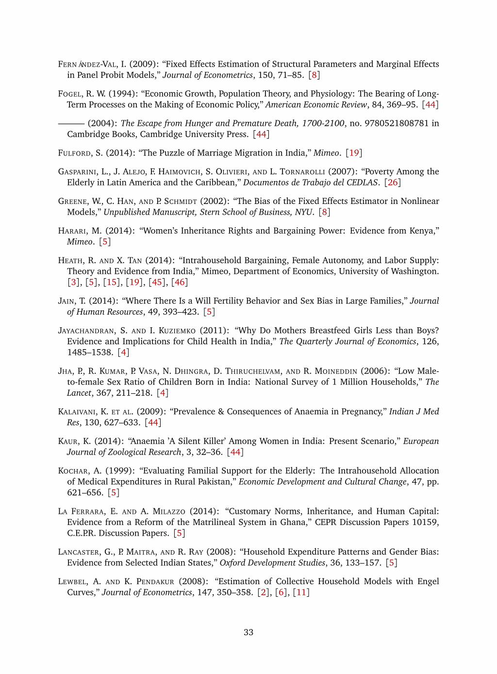
FERNÁNDEZ-VAL, I. (2009): “Fixed Effects Estimation of Structural Parameters and Marginal Effectsin Panel Probit Models,” Journal of Econometrics, 150, 71–85. [8]

FOGEL, R. W. (1994): “Economic Growth, Population Theory, and Physiology: The Bearing of Long-Term Processes on the Making of Economic Policy,” American Economic Review, 84, 369–95. [44]

——— (2004): The Escape from Hunger and Premature Death, 1700-2100, no. 9780521808781 inCambridge Books, Cambridge University Press. [44]

FULFORD, S. (2014): “The Puzzle of Marriage Migration in India,” Mimeo. [19]

GASPARINI, L., J. ALEJO, F. HAIMOVICH, S. OLIVIERI, AND L. TORNAROLLI (2007): “Poverty Among theElderly in Latin America and the Caribbean,” Documentos de Trabajo del CEDLAS. [26]

GREENE, W., C. HAN, AND P. SCHMIDT (2002): “The Bias of the Fixed Effects Estimator in NonlinearModels,” Unpublished Manuscript, Stern School of Business, NYU. [8]

HARARI, M. (2014): “Women’s Inheritance Rights and Bargaining Power: Evidence from Kenya,”Mimeo. [5]

HEATH, R. AND X. TAN (2014): “Intrahousehold Bargaining, Female Autonomy, and Labor Supply:Theory and Evidence from India,” Mimeo, Department of Economics, University of Washington.[3], [5], [15], [19], [45], [46]

JAIN, T. (2014): “Where There Is a Will Fertility Behavior and Sex Bias in Large Families,” Journalof Human Resources, 49, 393–423. [5]

JAYACHANDRAN, S. AND I. KUZIEMKO (2011): “Why Do Mothers Breastfeed Girls Less than Boys?Evidence and Implications for Child Health in India,” The Quarterly Journal of Economics, 126,1485–1538. [4]

JHA, P., R. KUMAR, P. VASA, N. DHINGRA, D. THIRUCHELVAM, AND R. MOINEDDIN (2006): “Low Male-to-female Sex Ratio of Children Born in India: National Survey of 1 Million Households,” TheLancet, 367, 211–218. [4]

KALAIVANI, K. ET AL. (2009): “Prevalence & Consequences of Anaemia in Pregnancy,” Indian J MedRes, 130, 627–633. [44]

KAUR, K. (2014): “Anaemia ’A Silent Killer’ Among Women in India: Present Scenario,” EuropeanJournal of Zoological Research, 3, 32–36. [44]

KOCHAR, A. (1999): “Evaluating Familial Support for the Elderly: The Intrahousehold Allocationof Medical Expenditures in Rural Pakistan,” Economic Development and Cultural Change, 47, pp.621–656. [5]

LA FERRARA, E. AND A. MILAZZO (2014): “Customary Norms, Inheritance, and Human Capital:Evidence from a Reform of the Matrilineal System in Ghana,” CEPR Discussion Papers 10159,C.E.P.R. Discussion Papers. [5]

LANCASTER, G., P. MAITRA, AND R. RAY (2008): “Household Expenditure Patterns and Gender Bias:Evidence from Selected Indian States,” Oxford Development Studies, 36, 133–157. [5]

LEWBEL, A. AND K. PENDAKUR (2008): “Estimation of Collective Household Models with EngelCurves,” Journal of Econometrics, 147, 350–358. [2], [6], [11]

33

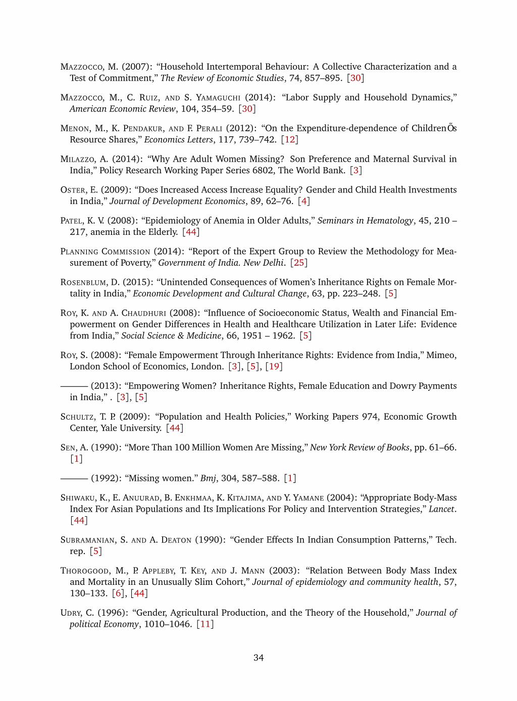
MAZZOCCO, M. (2007): “Household Intertemporal Behaviour: A Collective Characterization and aTest of Commitment,” The Review of Economic Studies, 74, 857–895. [30]

MAZZOCCO, M., C. RUIZ, AND S. YAMAGUCHI (2014): “Labor Supply and Household Dynamics,”American Economic Review, 104, 354–59. [30]

MENON, M., K. PENDAKUR, AND F. PERALI (2012): “On the Expenditure-dependence of ChildrenÕsResource Shares,” Economics Letters, 117, 739–742. [12]

MILAZZO, A. (2014): “Why Are Adult Women Missing? Son Preference and Maternal Survival inIndia,” Policy Research Working Paper Series 6802, The World Bank. [3]

OSTER, E. (2009): “Does Increased Access Increase Equality? Gender and Child Health Investmentsin India,” Journal of Development Economics, 89, 62–76. [4]

PATEL, K. V. (2008): “Epidemiology of Anemia in Older Adults,” Seminars in Hematology, 45, 210 –217, anemia in the Elderly. [44]

PLANNING COMMISSION (2014): “Report of the Expert Group to Review the Methodology for Mea-surement of Poverty,” Government of India. New Delhi. [25]

ROSENBLUM, D. (2015): “Unintended Consequences of Women’s Inheritance Rights on Female Mor-tality in India,” Economic Development and Cultural Change, 63, pp. 223–248. [5]

ROY, K. AND A. CHAUDHURI (2008): “Influence of Socioeconomic Status, Wealth and Financial Em-powerment on Gender Differences in Health and Healthcare Utilization in Later Life: Evidencefrom India,” Social Science & Medicine, 66, 1951 – 1962. [5]

ROY, S. (2008): “Female Empowerment Through Inheritance Rights: Evidence from India,” Mimeo,London School of Economics, London. [3], [5], [19]

——— (2013): “Empowering Women? Inheritance Rights, Female Education and Dowry Paymentsin India,” . [3], [5]

SCHULTZ, T. P. (2009): “Population and Health Policies,” Working Papers 974, Economic GrowthCenter, Yale University. [44]

SEN, A. (1990): “More Than 100 Million Women Are Missing,” New York Review of Books, pp. 61–66.[1]

——— (1992): “Missing women.” Bmj, 304, 587–588. [1]

SHIWAKU, K., E. ANUURAD, B. ENKHMAA, K. KITAJIMA, AND Y. YAMANE (2004): “Appropriate Body-MassIndex For Asian Populations and Its Implications For Policy and Intervention Strategies,” Lancet.[44]

SUBRAMANIAN, S. AND A. DEATON (1990): “Gender Effects In Indian Consumption Patterns,” Tech.rep. [5]

THOROGOOD, M., P. APPLEBY, T. KEY, AND J. MANN (2003): “Relation Between Body Mass Indexand Mortality in an Unusually Slim Cohort,” Journal of epidemiology and community health, 57,130–133. [6], [44]

UDRY, C. (1996): “Gender, Agricultural Production, and the Theory of the Household,” Journal ofpolitical Economy, 1010–1046. [11]

34

VERMEULEN, F. (2002): “Collective Household Models: Principles and Main Results,” Journal ofEconomic Surveys, 16, 533–564. [6], [11]

VISSCHER, T. L. S., J. C. SEIDELL, A. MENOTTI, H. BLACKBURN, A. NISSINEN, E. J. M. FESKENS,D. KROMHOUT, AND FOR THE SEVEN COUNTRIES STUDY RESEARCH GROUP (2000): “Underweightand Overweight in Relation to Mortality Among Men Aged 40-59 and 50-69 Years: The SevenCountries Study,” American Journal of Epidemiology, 151, 660–666. [6], [44]

VOENA, A. (2015): “Yours, Mine, and Ours: Do Divorce Laws Affect the Intertemporal Behavior ofMarried Couples?” American Economic Review, 105, 2295–2332. [16], [30]

WAILER, H. T. (1984): “Height, Weight and Mortality: The Norwegian Experience,” Acta MedicaScandinavica, 215, 1–56. [44]

WORLD BANK (2014): “Women, Business and the Law 2014. Removing Restrictions to EnhanceGender Equality,” World Bank Report. [6]

WORLD HEALTH ORGANIZATION (1999): World Health Report 1999 - Making a Difference, WorldHealth Organization. [2]

——— (2015): World Health Statistics 2015, World Health Organization. [2]

ZHENG, W., D. F. MCLERRAN, B. ROLLAND, X. ZHANG, M. INOUE, K. MATSUO, J. HE, P. C. GUPTA, K. RA-MADAS, S. TSUGANE, ET AL. (2011): “Association Between Body-mass Index and Risk of Death inMore than 1 million Asians,” New England Journal of Medicine, 364, 719–729. [6], [44]

ZIMMERMANN, L. (2012): “Reconsidering Gender Bias in Intrahousehold Allocation in India,” Jour-nal of Development Studies, 48, 151–163. [5]

A Appendix

This Appendix contains seven main sections. Appendix A.1 shows that the recent findings about

missing Indian women at older ages are consistent with the distribution of sex-ratios across ages.

Appendix A.2 contains additional tables and figures. Appendix A.3 presents the full empirical anal-

ysis of the effect of the Hindu Succession Act amendments on women’s health and details on the

dataset used, the empirical strategy and the robustness checks. Appendix A.4 discusses a fully

specified collective model of Indian households. While invoking additional functional forms that

are not required for the empirical estimation of the resource shares, the fully specified model de-

livers explicit formulas for household demands and resource shares that satisfy the identification

requirements. Appendix A.5 investigates the sensitivity of the model estimates. Appendix A.6 uses

additional data on singles to empirically test the Pareto efficiency assumption in this framework.

Appendix A.7 relaxes the assumption of equality of poverty thresholds between genders and simu-

lates gender and gender-age poverty rates in this alternative scenario.

35

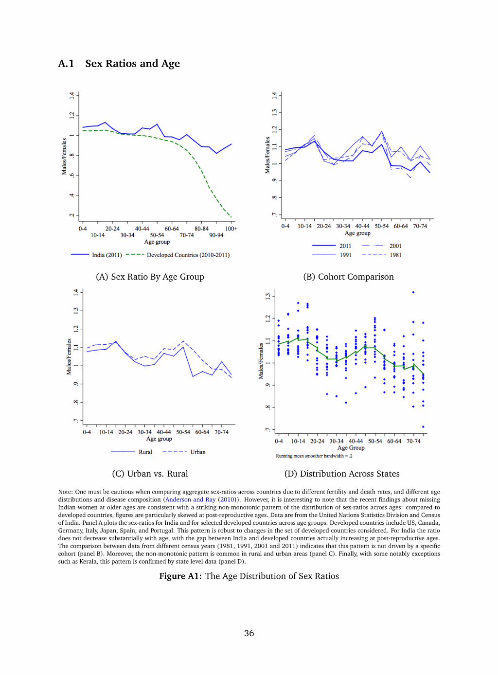
A.1 Sex Ratios and Age

(A) Sex Ratio By Age Group (B) Cohort Comparison

(C) Urban vs. Rural (D) Distribution Across States

Note: One must be cautious when comparing aggregate sex-ratios across countries due to different fertility and death rates, and different agedistributions and disease composition (Anderson and Ray (2010)). However, it is interesting to note that the recent findings about missingIndian women at older ages are consistent with a striking non-monotonic pattern of the distribution of sex-ratios across ages: compared todeveloped countries, figures are particularly skewed at post-reproductive ages. Data are from the United Nations Statistics Division and Censusof India. Panel A plots the sex-ratios for India and for selected developed countries across age groups. Developed countries include US, Canada,Germany, Italy, Japan, Spain, and Portugal. This pattern is robust to changes in the set of developed countries considered. For India the ratiodoes not decrease substantially with age, with the gap between India and developed countries actually increasing at post-reproductive ages.The comparison between data from different census years (1981, 1991, 2001 and 2011) indicates that this pattern is not driven by a specificcohort (panel B). Moreover, the non-monotonic pattern is common in rural and urban areas (panel C). Finally, with some notably exceptionssuch as Kerala, this pattern is confirmed by state level data (panel D).

Figure A1: The Age Distribution of Sex Ratios

36

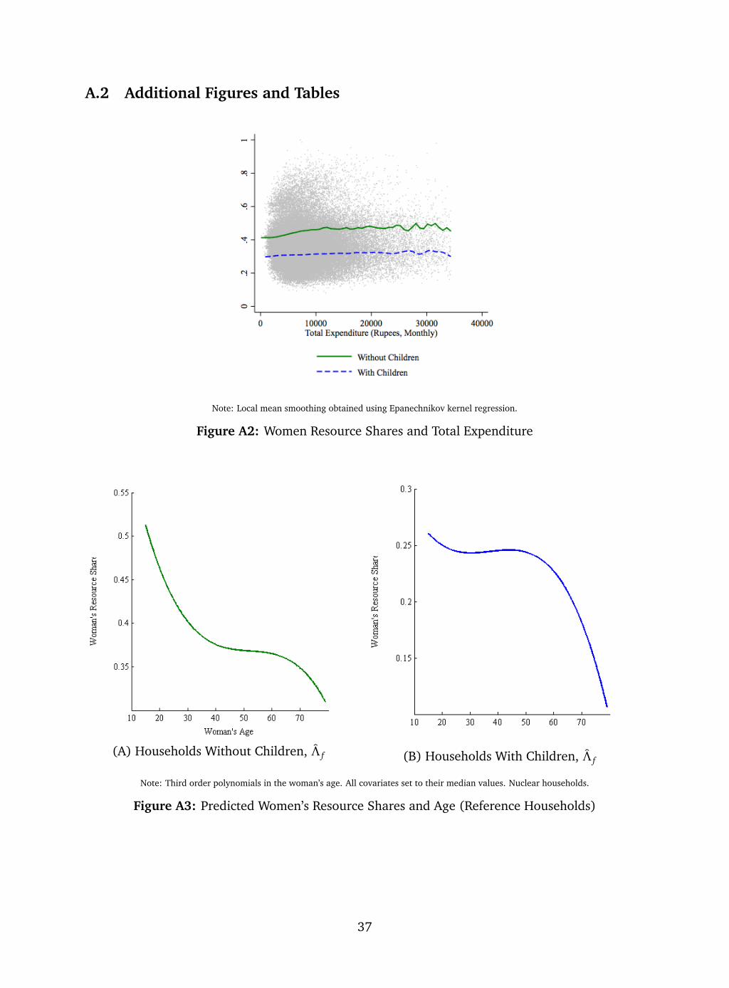
A.2 Additional Figures and Tables

Note: Local mean smoothing obtained using Epanechnikov kernel regression.

Figure A2: Women Resource Shares and Total Expenditure

(A) Households Without Children, Λ f (B) Households With Children, Λ f

Note: Third order polynomials in the woman’s age. All covariates set to their median values. Nuclear households.

Figure A3: Predicted Women’s Resource Shares and Age (Reference Households)

37

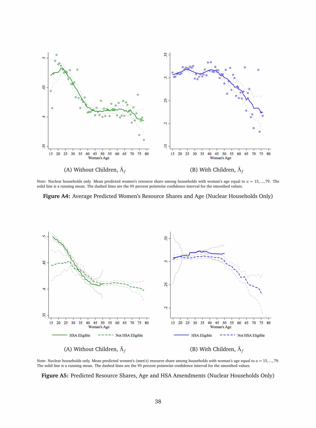
(A) Without Children, Λ f (B) With Children, Λ f

Note: Nuclear households only. Mean predicted women’s resource share among households with woman’s age equal to a = 15, ..., 79. Thesolid line is a running mean. The dashed lines are the 95 percent pointwise confidence interval for the smoothed values.

Figure A4: Average Predicted Women’s Resource Shares and Age (Nuclear Households Only)

(A) Without Children, Λ f (B) With Children, Λ f

Note: Nuclear households only. Mean predicted women’s (men’s) resource share among households with woman’s age equal to a = 15, ..., 79.The solid line is a running mean. The dashed lines are the 95 percent pointwise confidence interval for the smoothed values.

Figure A5: Predicted Resource Shares, Age and HSA Amendments (Nuclear Households Only)

38

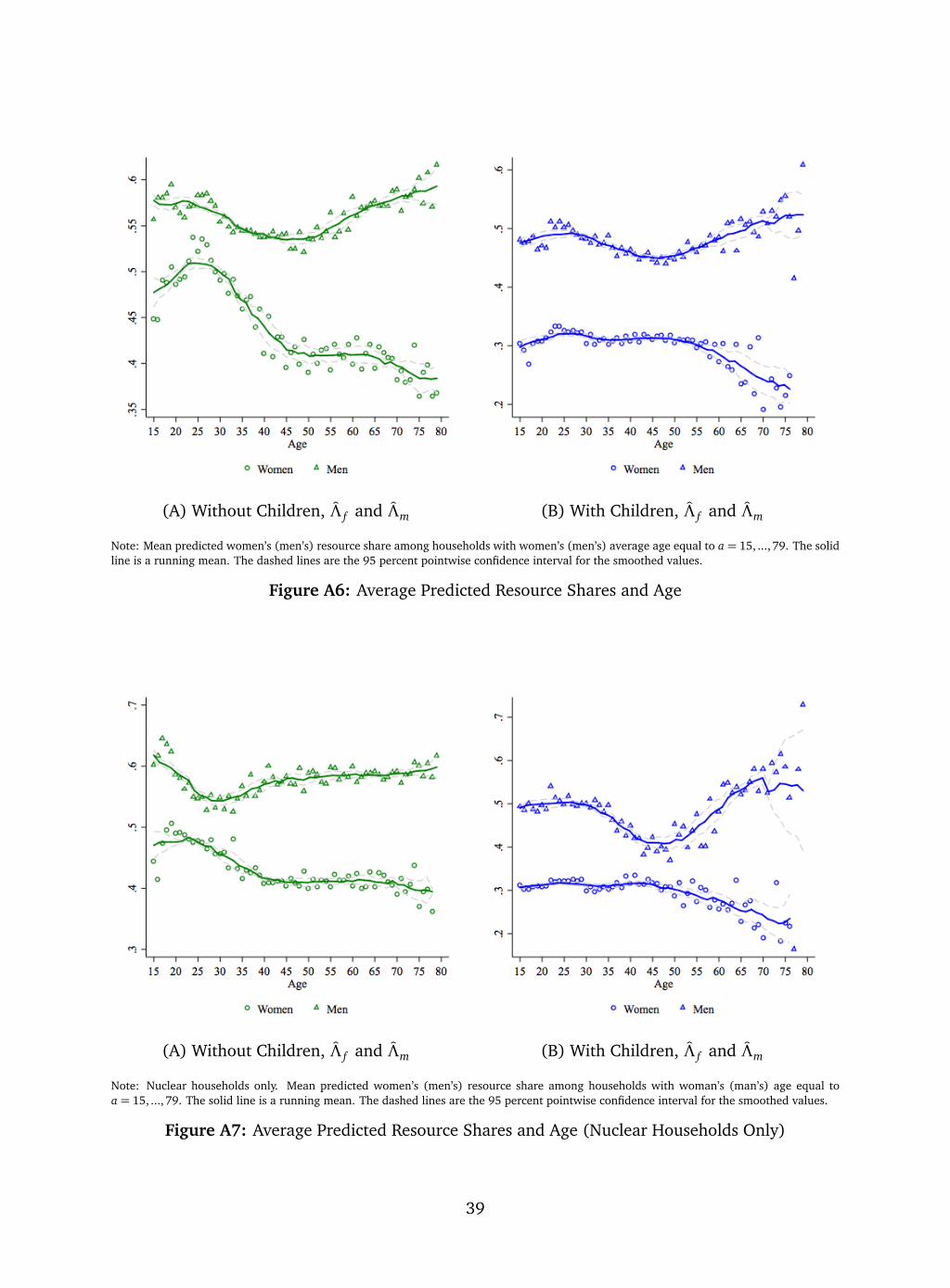
(A) Without Children, Λ f and Λm (B) With Children, Λ f and Λm

Note: Mean predicted women’s (men’s) resource share among households with women’s (men’s) average age equal to a = 15, ..., 79. The solidline is a running mean. The dashed lines are the 95 percent pointwise confidence interval for the smoothed values.

Figure A6: Average Predicted Resource Shares and Age

(A) Without Children, Λ f and Λm (B) With Children, Λ f and Λm

Note: Nuclear households only. Mean predicted women’s (men’s) resource share among households with woman’s (man’s) age equal toa = 15, ..., 79. The solid line is a running mean. The dashed lines are the 95 percent pointwise confidence interval for the smoothed values.

Figure A7: Average Predicted Resource Shares and Age (Nuclear Households Only)

39

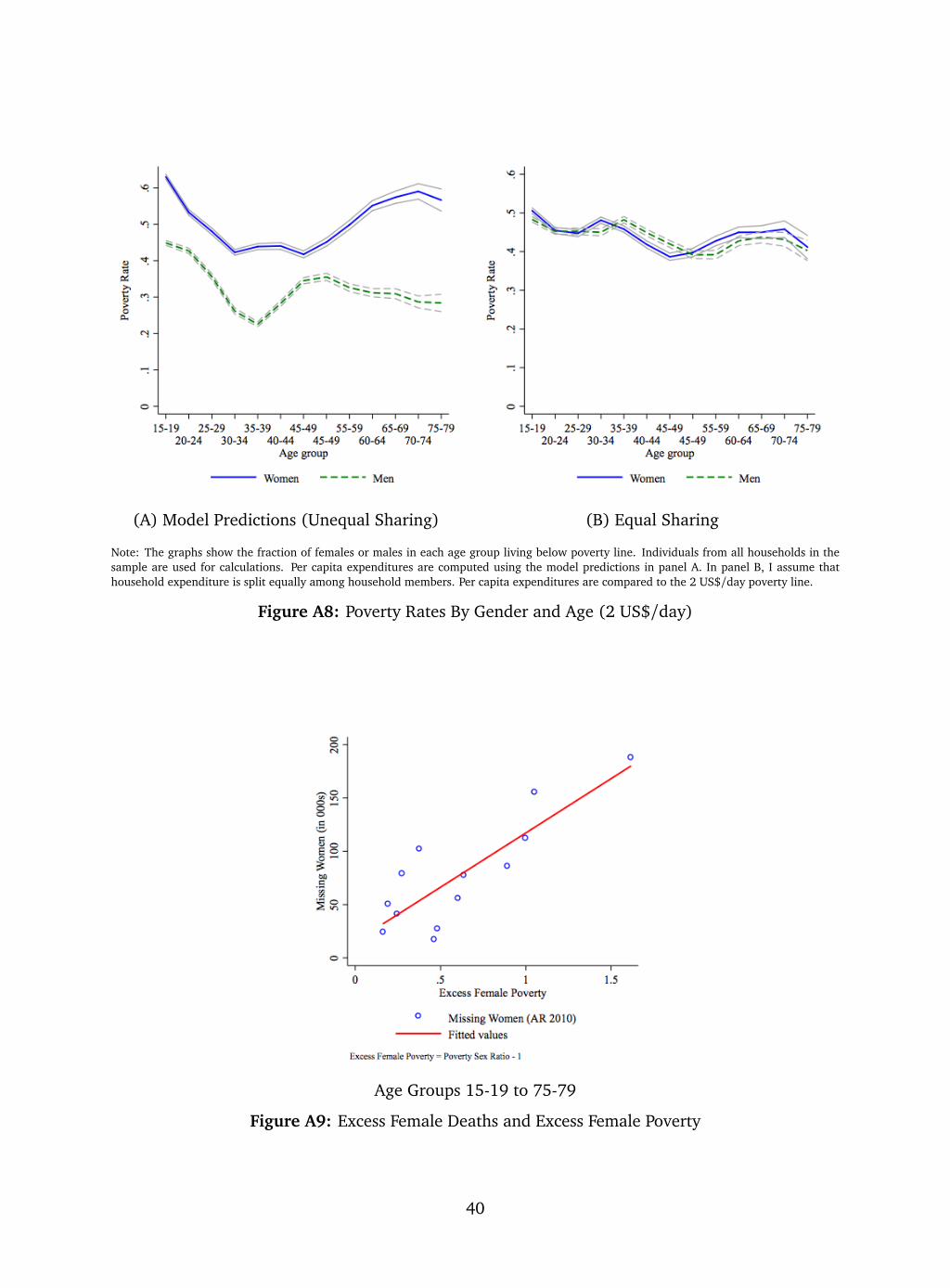
(A) Model Predictions (Unequal Sharing) (B) Equal Sharing

Note: The graphs show the fraction of females or males in each age group living below poverty line. Individuals from all households in thesample are used for calculations. Per capita expenditures are computed using the model predictions in panel A. In panel B, I assume thathousehold expenditure is split equally among household members. Per capita expenditures are compared to the 2 US$/day poverty line.

Figure A8: Poverty Rates By Gender and Age (2 US$/day)

Age Groups 15-19 to 75-79

Figure A9: Excess Female Deaths and Excess Female Poverty

40

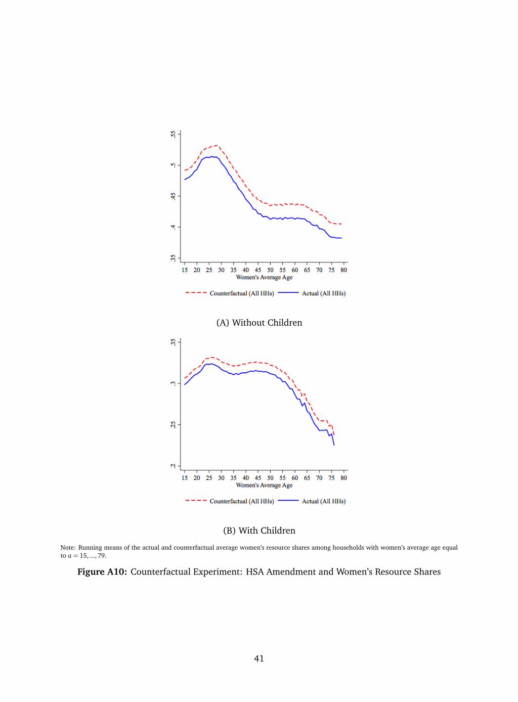
(A) Without Children

(B) With Children

Note: Running means of the actual and counterfactual average women’s resource shares among households with women’s average age equalto a = 15, ..., 79.

Figure A10: Counterfactual Experiment: HSA Amendment and Women’s Resource Shares

41

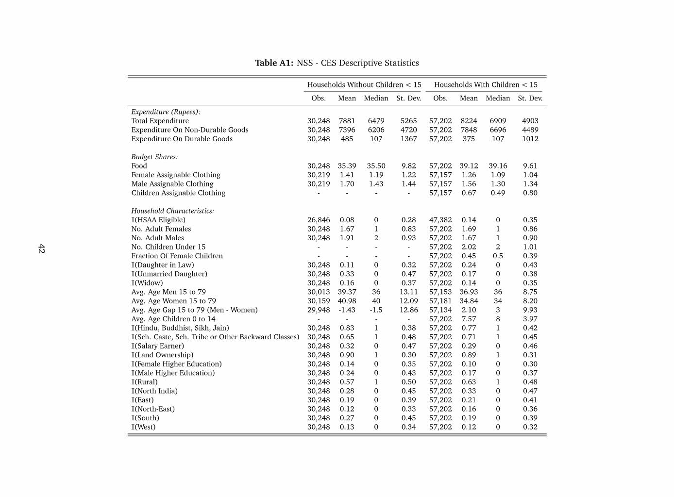
Table A1: NSS - CES Descriptive Statistics

Households Without Children < 15 Households With Children < 15

Obs. Mean Median St. Dev. Obs. Mean Median St. Dev.

Expenditure (Rupees):Total Expenditure 30,248 7881 6479 5265 57,202 8224 6909 4903Expenditure On Non-Durable Goods 30,248 7396 6206 4720 57,202 7848 6696 4489Expenditure On Durable Goods 30,248 485 107 1367 57,202 375 107 1012

Budget Shares:Food 30,248 35.39 35.50 9.82 57,202 39.12 39.16 9.61Female Assignable Clothing 30,219 1.41 1.19 1.22 57,157 1.26 1.09 1.04Male Assignable Clothing 30,219 1.70 1.43 1.44 57,157 1.56 1.30 1.34Children Assignable Clothing - - - - 57,157 0.67 0.49 0.80

Household Characteristics:I(HSAA Eligible) 26,846 0.08 0 0.28 47,382 0.14 0 0.35No. Adult Females 30,248 1.67 1 0.83 57,202 1.69 1 0.86No. Adult Males 30,248 1.91 2 0.93 57,202 1.67 1 0.90No. Children Under 15 - - - - 57,202 2.02 2 1.01Fraction Of Female Children - - - - 57,202 0.45 0.5 0.39I(Daughter in Law) 30,248 0.11 0 0.32 57,202 0.24 0 0.43I(Unmarried Daughter) 30,248 0.33 0 0.47 57,202 0.17 0 0.38I(Widow) 30,248 0.16 0 0.37 57,202 0.14 0 0.35Avg. Age Men 15 to 79 30,013 39.37 36 13.11 57,153 36.93 36 8.75Avg. Age Women 15 to 79 30,159 40.98 40 12.09 57,181 34.84 34 8.20Avg. Age Gap 15 to 79 (Men - Women) 29,948 -1.43 -1.5 12.86 57,134 2.10 3 9.93Avg. Age Children 0 to 14 - - - - 57,202 7.57 8 3.97I(Hindu, Buddhist, Sikh, Jain) 30,248 0.83 1 0.38 57,202 0.77 1 0.42I(Sch. Caste, Sch. Tribe or Other Backward Classes) 30,248 0.65 1 0.48 57,202 0.71 1 0.45I(Salary Earner) 30,248 0.32 0 0.47 57,202 0.29 0 0.46I(Land Ownership) 30,248 0.90 1 0.30 57,202 0.89 1 0.31I(Female Higher Education) 30,248 0.14 0 0.35 57,202 0.10 0 0.30I(Male Higher Education) 30,248 0.24 0 0.43 57,202 0.17 0 0.37I(Rural) 30,248 0.57 1 0.50 57,202 0.63 1 0.48I(North India) 30,248 0.28 0 0.45 57,202 0.33 0 0.47I(East) 30,248 0.19 0 0.39 57,202 0.21 0 0.41I(North-East) 30,248 0.12 0 0.33 57,202 0.16 0 0.36I(South) 30,248 0.27 0 0.45 57,202 0.19 0 0.39I(West) 30,248 0.13 0 0.34 57,202 0.12 0 0.32

42

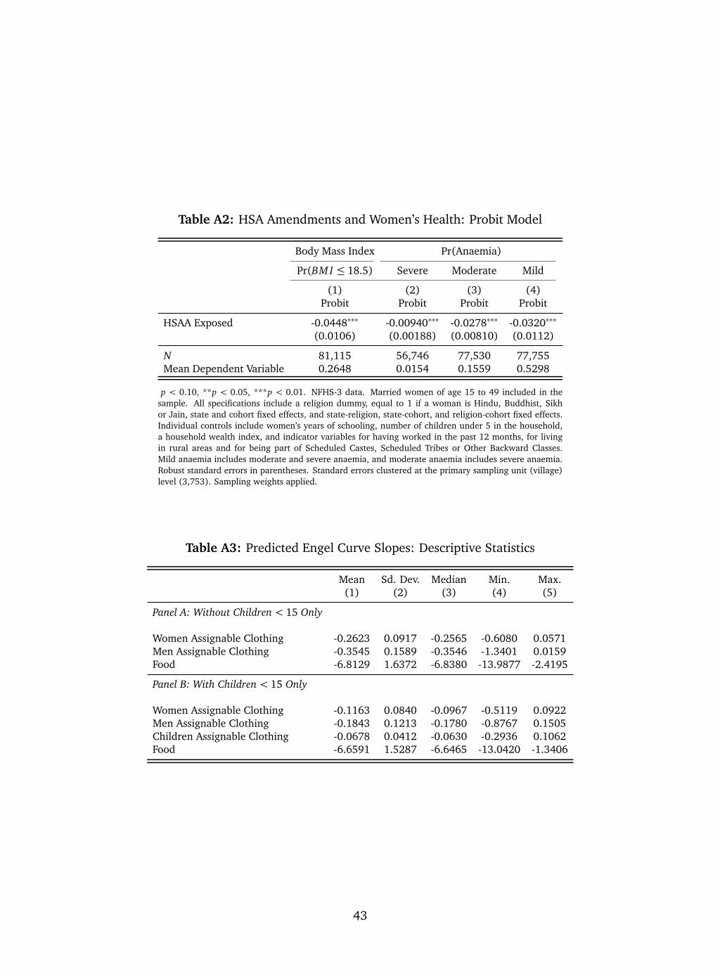
Table A2: HSA Amendments and Women’s Health: Probit Model

Body Mass Index Pr(Anaemia)

Pr(BM I ≤ 18.5) Severe Moderate Mild

(1) (2) (3) (4)Probit Probit Probit Probit

HSAA Exposed -0.0448∗∗∗ -0.00940∗∗∗ -0.0278∗∗∗ -0.0320∗∗∗

(0.0106) (0.00188) (0.00810) (0.0112)

N 81,115 56,746 77,530 77,755Mean Dependent Variable 0.2648 0.0154 0.1559 0.5298

p < 0.10, **p < 0.05, ***p < 0.01. NFHS-3 data. Married women of age 15 to 49 included in thesample. All specifications include a religion dummy, equal to 1 if a woman is Hindu, Buddhist, Sikhor Jain, state and cohort fixed effects, and state-religion, state-cohort, and religion-cohort fixed effects.Individual controls include women’s years of schooling, number of children under 5 in the household,a household wealth index, and indicator variables for having worked in the past 12 months, for livingin rural areas and for being part of Scheduled Castes, Scheduled Tribes or Other Backward Classes.Mild anaemia includes moderate and severe anaemia, and moderate anaemia includes severe anaemia.Robust standard errors in parentheses. Standard errors clustered at the primary sampling unit (village)level (3,753). Sampling weights applied.

Table A3: Predicted Engel Curve Slopes: Descriptive Statistics

Mean Sd. Dev. Median Min. Max.(1) (2) (3) (4) (5)

Panel A: Without Children < 15 Only

Women Assignable Clothing -0.2623 0.0917 -0.2565 -0.6080 0.0571Men Assignable Clothing -0.3545 0.1589 -0.3546 -1.3401 0.0159Food -6.8129 1.6372 -6.8380 -13.9877 -2.4195

Panel B: With Children < 15 Only

Women Assignable Clothing -0.1163 0.0840 -0.0967 -0.5119 0.0922Men Assignable Clothing -0.1843 0.1213 -0.1780 -0.8767 0.1505Children Assignable Clothing -0.0678 0.0412 -0.0630 -0.2936 0.1062Food -6.6591 1.5287 -6.6465 -13.0420 -1.3406

43

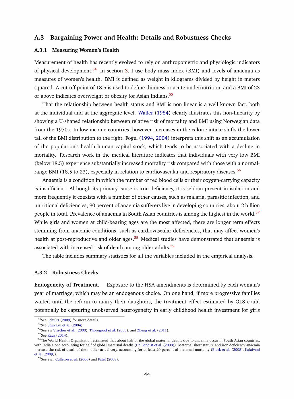
A.3 Bargaining Power and Health: Details and Robustness Checks

A.3.1 Measuring Women’s Health

Measurement of health has recently evolved to rely on anthropometric and physiologic indicators

of physical development.54 In section 3, I use body mass index (BMI) and levels of anaemia as

measures of women’s health. BMI is defined as weight in kilograms divided by height in meters

squared. A cut-off point of 18.5 is used to define thinness or acute undernutrition, and a BMI of 23

or above indicates overweight or obesity for Asian Indians.55

That the relationship between health status and BMI is non-linear is a well known fact, both

at the individual and at the aggregate level. Wailer (1984) clearly illustrates this non-linearity by

showing a U-shaped relationship between relative risk of mortality and BMI using Norwegian data

from the 1970s. In low income countries, however, increases in the caloric intake shifts the lower

tail of the BMI distribution to the right. Fogel (1994, 2004) interprets this shift as an accumulation

of the population’s health human capital stock, which tends to be associated with a decline in

mortality. Research work in the medical literature indicates that individuals with very low BMI

(below 18.5) experience substantially increased mortality risk compared with those with a normal-

range BMI (18.5 to 23), especially in relation to cardiovascular and respiratory diseases.56

Anaemia is a condition in which the number of red blood cells or their oxygen-carrying capacity

is insufficient. Although its primary cause is iron deficiency, it is seldom present in isolation and

more frequently it coexists with a number of other causes, such as malaria, parasitic infection, and

nutritional deficiencies; 90 percent of anaemia sufferers live in developing countries, about 2 billion

people in total. Prevalence of anaemia in South Asian countries is among the highest in the world.57

While girls and women at child-bearing ages are the most affected, there are longer term effects

stemming from anaemic conditions, such as cardiovascular deficiencies, that may affect women’s

health at post-reproductive and older ages.58 Medical studies have demonstrated that anaemia is

associated with increased risk of death among older adults.59

The table includes summary statistics for all the variables included in the empirical analysis.

A.3.2 Robustness Checks

Endogeneity of Treatment. Exposure to the HSA amendments is determined by each woman’s

year of marriage, which may be an endogenous choice. On one hand, if more progressive families

waited until the reform to marry their daughters, the treatment effect estimated by OLS could

potentially be capturing unobserved heterogeneity in early childhood health investment for girls

54See Schultz (2009) for more details.55See Shiwaku et al. (2004).56See e.g Visscher et al. (2000), Thorogood et al. (2003), and Zheng et al. (2011).57See Kaur (2014).58The World Health Organization estimated that about half of the global maternal deaths due to anaemia occur in South Asian countries,

with India alone accounting for half of global maternal deaths (De Benoist et al. (2008)). Maternal short stature and iron deficiency anaemiaincrease the risk of death of the mother at delivery, accounting for at least 20 percent of maternal mortality (Black et al. (2008), Kalaivaniet al. (2009)).

59See e.g., Culleton et al. (2006) and Patel (2008).

44

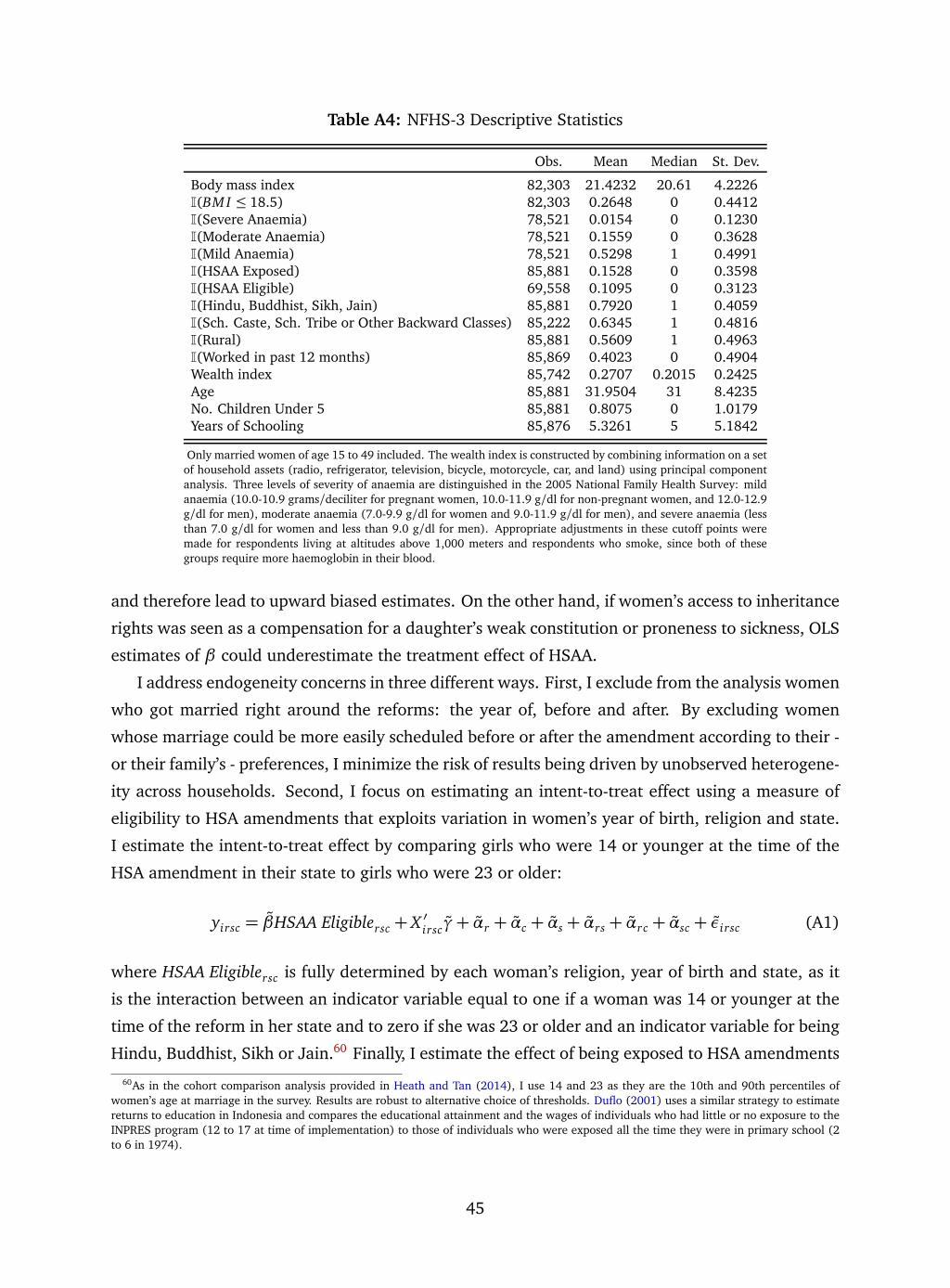
Table A4: NFHS-3 Descriptive Statistics

Obs. Mean Median St. Dev.

Body mass index 82,303 21.4232 20.61 4.2226I(BM I ≤ 18.5) 82,303 0.2648 0 0.4412I(Severe Anaemia) 78,521 0.0154 0 0.1230I(Moderate Anaemia) 78,521 0.1559 0 0.3628I(Mild Anaemia) 78,521 0.5298 1 0.4991I(HSAA Exposed) 85,881 0.1528 0 0.3598I(HSAA Eligible) 69,558 0.1095 0 0.3123I(Hindu, Buddhist, Sikh, Jain) 85,881 0.7920 1 0.4059I(Sch. Caste, Sch. Tribe or Other Backward Classes) 85,222 0.6345 1 0.4816I(Rural) 85,881 0.5609 1 0.4963I(Worked in past 12 months) 85,869 0.4023 0 0.4904Wealth index 85,742 0.2707 0.2015 0.2425Age 85,881 31.9504 31 8.4235No. Children Under 5 85,881 0.8075 0 1.0179Years of Schooling 85,876 5.3261 5 5.1842

Only married women of age 15 to 49 included. The wealth index is constructed by combining information on a setof household assets (radio, refrigerator, television, bicycle, motorcycle, car, and land) using principal componentanalysis. Three levels of severity of anaemia are distinguished in the 2005 National Family Health Survey: mildanaemia (10.0-10.9 grams/deciliter for pregnant women, 10.0-11.9 g/dl for non-pregnant women, and 12.0-12.9g/dl for men), moderate anaemia (7.0-9.9 g/dl for women and 9.0-11.9 g/dl for men), and severe anaemia (lessthan 7.0 g/dl for women and less than 9.0 g/dl for men). Appropriate adjustments in these cutoff points weremade for respondents living at altitudes above 1,000 meters and respondents who smoke, since both of thesegroups require more haemoglobin in their blood.

and therefore lead to upward biased estimates. On the other hand, if women’s access to inheritance

rights was seen as a compensation for a daughter’s weak constitution or proneness to sickness, OLS

estimates of β could underestimate the treatment effect of HSAA.

I address endogeneity concerns in three different ways. First, I exclude from the analysis women

who got married right around the reforms: the year of, before and after. By excluding women

whose marriage could be more easily scheduled before or after the amendment according to their -

or their family’s - preferences, I minimize the risk of results being driven by unobserved heterogene-

ity across households. Second, I focus on estimating an intent-to-treat effect using a measure of

eligibility to HSA amendments that exploits variation in women’s year of birth, religion and state.

I estimate the intent-to-treat effect by comparing girls who were 14 or younger at the time of the

HSA amendment in their state to girls who were 23 or older:

yirsc = βHSAA Eligiblersc + X ′irscγ+ αr + αc + αs + αrs + αrc + αsc + εirsc (A1)

where HSAA Eligiblersc is fully determined by each woman’s religion, year of birth and state, as it

is the interaction between an indicator variable equal to one if a woman was 14 or younger at the

time of the reform in her state and to zero if she was 23 or older and an indicator variable for being

Hindu, Buddhist, Sikh or Jain.60 Finally, I estimate the effect of being exposed to HSA amendments

60As in the cohort comparison analysis provided in Heath and Tan (2014), I use 14 and 23 as they are the 10th and 90th percentiles ofwomen’s age at marriage in the survey. Results are robust to alternative choice of thresholds. Duflo (2001) uses a similar strategy to estimatereturns to education in Indonesia and compares the educational attainment and the wages of individuals who had little or no exposure to theINPRES program (12 to 17 at time of implementation) to those of individuals who were exposed all the time they were in primary school (2to 6 in 1974).

45

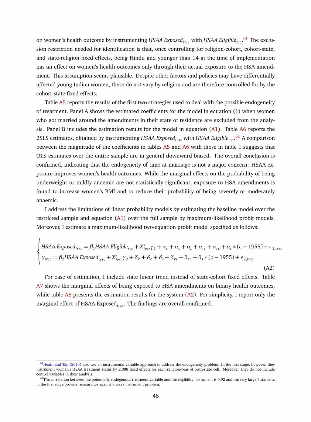
on women’s health outcome by instrumenting HSAA Exposedirsc with HSAA Eligiblersc.61 The exclu-

sion restriction needed for identification is that, once controlling for religion-cohort, cohort-state,

and state-religion fixed effects, being Hindu and younger than 14 at the time of implementation

has an effect on women’s health outcomes only through their actual exposure to the HSA amend-

ment. This assumption seems plausible. Despite other factors and policies may have differentially

affected young Indian women, these do not vary by religion and are therefore controlled for by the

cohort-state fixed effects.

Table A5 reports the results of the first two strategies used to deal with the possible endogeneity

of treatment. Panel A shows the estimated coefficients for the model in equation (1) when women

who got married around the amendments in their state of residence are excluded from the analy-

sis. Panel B includes the estimation results for the model in equation (A1). Table A6 reports the

2SLS estimates, obtained by instrumenting HSAA Exposedirsc with HSAA Eligiblersc.62 A comparison

between the magnitude of the coefficients in tables A5 and A6 with those in table 1 suggests that

OLS estimates over the entire sample are in general downward biased. The overall conclusion is

confirmed, indicating that the endogeneity of time at marriage is not a major concern: HSAA ex-

posure improves women’s health outcomes. While the marginal effects on the probability of being

underweight or mildly anaemic are not statistically significant, exposure to HSA amendments is

found to increase women’s BMI and to reduce their probability of being severely or moderately

anaemic.

I address the limitations of linear probability models by estimating the baseline model over the

restricted sample and equation (A1) over the full sample by maximum-likelihood probit models.

Moreover, I estimate a maximum-likelihood two-equation probit model specified as follows:

HSAA Exposedirsc = β1HSAA Eligiblersc + X ′irscγ1+αr +αc +αs +αrs +αrc +αs ∗ (c− 1955) + ε1,irsc

yirsc = β2HSAA Exposedirsc + X ′irscγ2+δr +δc +δs +δrs +δrc +δs ∗ (c− 1955) + ε2,irsc

(A2)

For ease of estimation, I include state linear trend instead of state-cohort fixed effects. Table

A7 shows the marginal effects of being exposed to HSA amendments on binary health outcomes,

while table A8 presents the estimation results for the system (A2). For simplicity, I report only the

marginal effect of HSAA Exposedirsc. The findings are overall confirmed.

61Heath and Tan (2014) also use an instrumental variable approach to address the endogeneity problem. In the first stage, however, theyinstrument woman’s HSAA treatment status by 2,088 fixed effects for each religion-year of birth-state cell. Moreover, they do not includecontrol variables in their analysis.

62The correlation between the potentially endogenous treatment variable and the eligibility instrument is 0.92 and the very large F statisticsin the first stage provide reassurance against a weak instrument problem.

46

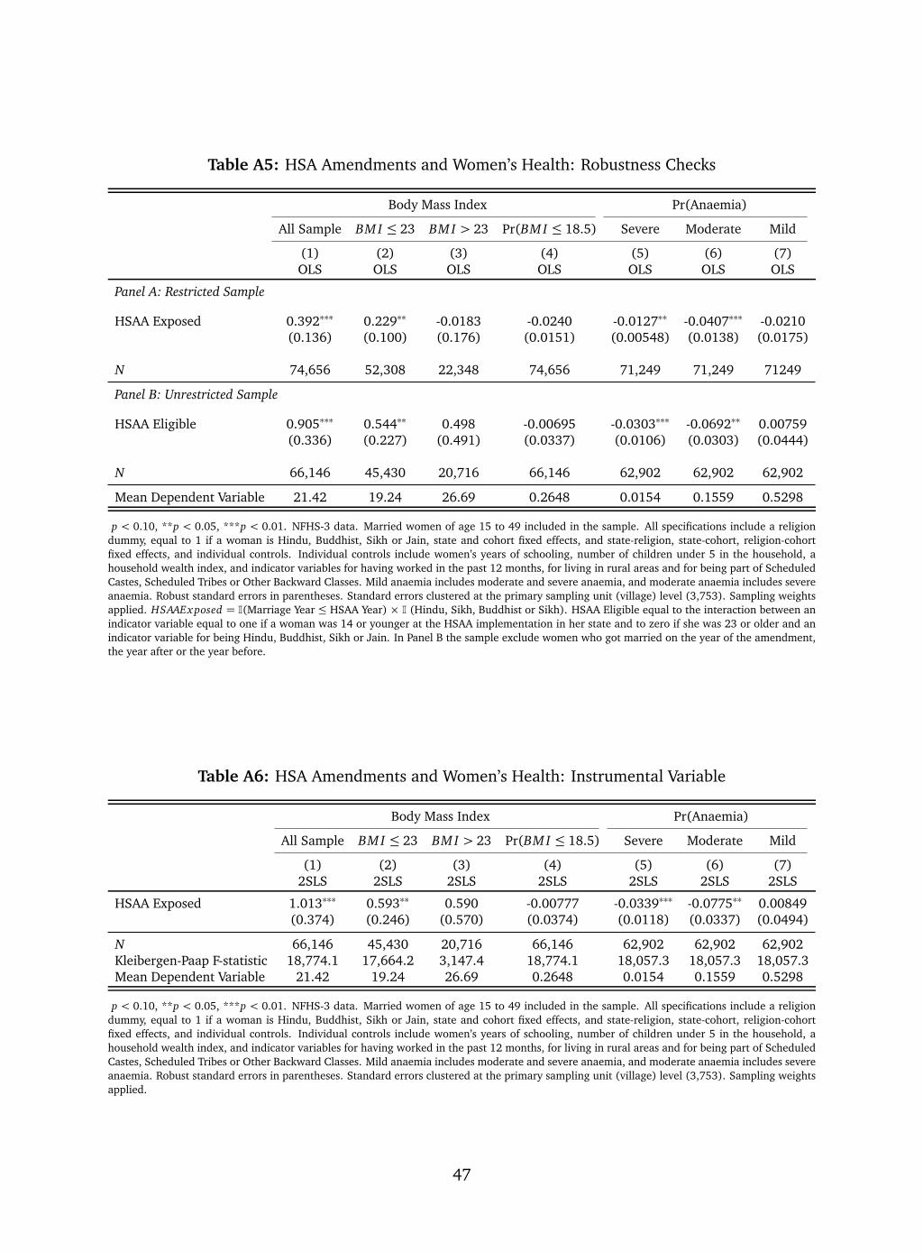
Table A5: HSA Amendments and Women’s Health: Robustness Checks

Body Mass Index Pr(Anaemia)

All Sample BM I ≤ 23 BM I > 23 Pr(BM I ≤ 18.5) Severe Moderate Mild

(1) (2) (3) (4) (5) (6) (7)OLS OLS OLS OLS OLS OLS OLS

Panel A: Restricted Sample

HSAA Exposed 0.392∗∗∗ 0.229∗∗ -0.0183 -0.0240 -0.0127∗∗ -0.0407∗∗∗ -0.0210(0.136) (0.100) (0.176) (0.0151) (0.00548) (0.0138) (0.0175)

N 74,656 52,308 22,348 74,656 71,249 71,249 71249

Panel B: Unrestricted Sample

HSAA Eligible 0.905∗∗∗ 0.544∗∗ 0.498 -0.00695 -0.0303∗∗∗ -0.0692∗∗ 0.00759(0.336) (0.227) (0.491) (0.0337) (0.0106) (0.0303) (0.0444)

N 66,146 45,430 20,716 66,146 62,902 62,902 62,902

Mean Dependent Variable 21.42 19.24 26.69 0.2648 0.0154 0.1559 0.5298

p < 0.10, **p < 0.05, ***p < 0.01. NFHS-3 data. Married women of age 15 to 49 included in the sample. All specifications include a religiondummy, equal to 1 if a woman is Hindu, Buddhist, Sikh or Jain, state and cohort fixed effects, and state-religion, state-cohort, religion-cohortfixed effects, and individual controls. Individual controls include women’s years of schooling, number of children under 5 in the household, ahousehold wealth index, and indicator variables for having worked in the past 12 months, for living in rural areas and for being part of ScheduledCastes, Scheduled Tribes or Other Backward Classes. Mild anaemia includes moderate and severe anaemia, and moderate anaemia includes severeanaemia. Robust standard errors in parentheses. Standard errors clustered at the primary sampling unit (village) level (3,753). Sampling weightsapplied. HSAAEx posed = I(Marriage Year ≤ HSAA Year) × I (Hindu, Sikh, Buddhist or Sikh). HSAA Eligible equal to the interaction between anindicator variable equal to one if a woman was 14 or younger at the HSAA implementation in her state and to zero if she was 23 or older and anindicator variable for being Hindu, Buddhist, Sikh or Jain. In Panel B the sample exclude women who got married on the year of the amendment,the year after or the year before.

Table A6: HSA Amendments and Women’s Health: Instrumental Variable

Body Mass Index Pr(Anaemia)

All Sample BM I ≤ 23 BM I > 23 Pr(BM I ≤ 18.5) Severe Moderate Mild

(1) (2) (3) (4) (5) (6) (7)2SLS 2SLS 2SLS 2SLS 2SLS 2SLS 2SLS

HSAA Exposed 1.013∗∗∗ 0.593∗∗ 0.590 -0.00777 -0.0339∗∗∗ -0.0775∗∗ 0.00849(0.374) (0.246) (0.570) (0.0374) (0.0118) (0.0337) (0.0494)

N 66,146 45,430 20,716 66,146 62,902 62,902 62,902Kleibergen-Paap F-statistic 18,774.1 17,664.2 3,147.4 18,774.1 18,057.3 18,057.3 18,057.3Mean Dependent Variable 21.42 19.24 26.69 0.2648 0.0154 0.1559 0.5298

p < 0.10, **p < 0.05, ***p < 0.01. NFHS-3 data. Married women of age 15 to 49 included in the sample. All specifications include a religiondummy, equal to 1 if a woman is Hindu, Buddhist, Sikh or Jain, state and cohort fixed effects, and state-religion, state-cohort, religion-cohortfixed effects, and individual controls. Individual controls include women’s years of schooling, number of children under 5 in the household, ahousehold wealth index, and indicator variables for having worked in the past 12 months, for living in rural areas and for being part of ScheduledCastes, Scheduled Tribes or Other Backward Classes. Mild anaemia includes moderate and severe anaemia, and moderate anaemia includes severeanaemia. Robust standard errors in parentheses. Standard errors clustered at the primary sampling unit (village) level (3,753). Sampling weightsapplied.

47

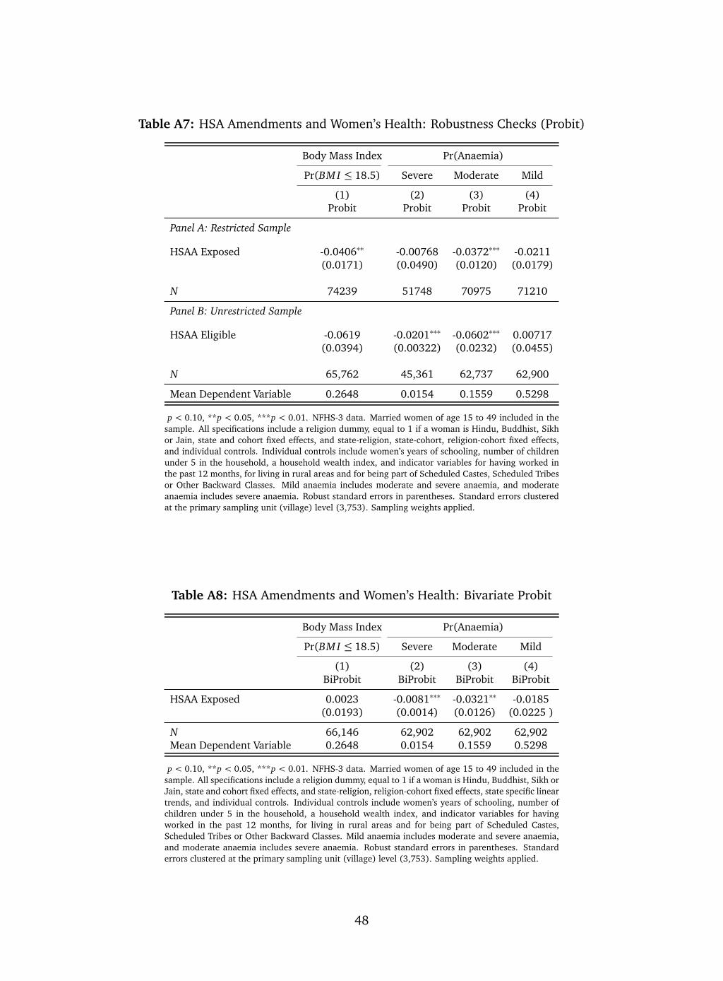
Table A7: HSA Amendments and Women’s Health: Robustness Checks (Probit)

Body Mass Index Pr(Anaemia)

Pr(BM I ≤ 18.5) Severe Moderate Mild

(1) (2) (3) (4)Probit Probit Probit Probit

Panel A: Restricted Sample

HSAA Exposed -0.0406∗∗ -0.00768 -0.0372∗∗∗ -0.0211(0.0171) (0.0490) (0.0120) (0.0179)

N 74239 51748 70975 71210

Panel B: Unrestricted Sample

HSAA Eligible -0.0619 -0.0201∗∗∗ -0.0602∗∗∗ 0.00717(0.0394) (0.00322) (0.0232) (0.0455)

N 65,762 45,361 62,737 62,900

Mean Dependent Variable 0.2648 0.0154 0.1559 0.5298

p < 0.10, **p < 0.05, ***p < 0.01. NFHS-3 data. Married women of age 15 to 49 included in thesample. All specifications include a religion dummy, equal to 1 if a woman is Hindu, Buddhist, Sikhor Jain, state and cohort fixed effects, and state-religion, state-cohort, religion-cohort fixed effects,and individual controls. Individual controls include women’s years of schooling, number of childrenunder 5 in the household, a household wealth index, and indicator variables for having worked inthe past 12 months, for living in rural areas and for being part of Scheduled Castes, Scheduled Tribesor Other Backward Classes. Mild anaemia includes moderate and severe anaemia, and moderateanaemia includes severe anaemia. Robust standard errors in parentheses. Standard errors clusteredat the primary sampling unit (village) level (3,753). Sampling weights applied.

Table A8: HSA Amendments and Women’s Health: Bivariate Probit

Body Mass Index Pr(Anaemia)

Pr(BM I ≤ 18.5) Severe Moderate Mild

(1) (2) (3) (4)BiProbit BiProbit BiProbit BiProbit

HSAA Exposed 0.0023 -0.0081∗∗∗ -0.0321∗∗ -0.0185(0.0193) (0.0014) (0.0126) (0.0225 )

N 66,146 62,902 62,902 62,902Mean Dependent Variable 0.2648 0.0154 0.1559 0.5298

p < 0.10, **p < 0.05, ***p < 0.01. NFHS-3 data. Married women of age 15 to 49 included in thesample. All specifications include a religion dummy, equal to 1 if a woman is Hindu, Buddhist, Sikh orJain, state and cohort fixed effects, and state-religion, religion-cohort fixed effects, state specific lineartrends, and individual controls. Individual controls include women’s years of schooling, number ofchildren under 5 in the household, a household wealth index, and indicator variables for havingworked in the past 12 months, for living in rural areas and for being part of Scheduled Castes,Scheduled Tribes or Other Backward Classes. Mild anaemia includes moderate and severe anaemia,and moderate anaemia includes severe anaemia. Robust standard errors in parentheses. Standarderrors clustered at the primary sampling unit (village) level (3,753). Sampling weights applied.

48

Falsification Tests. In order to assess the validity of my identification strategy, I perform two

different falsification tests. First, I compare health outcomes of younger and older women, who

could not be exposed to HSA amendments as they were too old at the time of implementation. In

particular, I estimate the specification in equation (A1) with the main regressor being the interac-

tion between an indicator variable equal to one if a woman was 23 to 30 years old at the time of

the HSA Amendment in her state and to zero if she was 30 or older, and an indicator variable for

being Hindu, Buddhist, Sikh or Jain. If there was a difference in trends between the reformed and

non-reformed states, I would find a statistically significant and positive coefficient on the newly de-

fined interaction term. This could cast doubt on the validity of the identification strategy discussed

above. Second, I estimate the effect of HSA Amendments on men’s health outcome. I combine

data on BMI, anemia level and demographic characteristics for adult males with information about

women’s eligibility within a household and I estimate the model in equation (A1) with the depen-

dent variable now being males’ health outcomes. If there was a general increasing trend common

to Hindu individuals, both men and women, in the reforming states, the estimated treatment effect

would be positive and significant for men as well.63

Table A9 contains the estimation results. For simplicity, the table reports only a subset of the

health outcomes considered above. Columns 1 to 4 show the estimation results for the model in

equation (A1) with the main regressor now being the interaction between an indicator variable

equal to one if a woman was 23 to 30 years old at the HSAA implementation in her state and to

zero if she was 30 or older, and an indicator variable for being Hindu, Buddhist, Sikh or Jain. I

find no significant effect on women’s BMI, on their probability of being underweight nor on their

probability of being anaemic, providing reassurance in favor of the validity of the empirical exercise.

Columns 5 to 8 report the estimation results for the model in equation (A1) when males’ health

outcomes are considered and the individual controls include males’ schooling and an indicator

variable for having worked in the past 12 months.64 The estimated coefficients and marginal effects

are not statistically different from zero, suggesting no violation of the identification assumptions.

63While an increase in men’s health could be rationalized by a change in expenditure patterns induced by the increase in women’s bargainingpower - for example for food and medical expenses -, evidence of it may cast doubt on the validity of the identification strategy.

64HSAA Eligible still refers to eligibility of the woman. Males’ health outcomes are taken from the NFHS-3 men surveys; each woman is thenmatched to a male respondent in her household. For simplicity, I retain information about only one male respondent in each household.

49

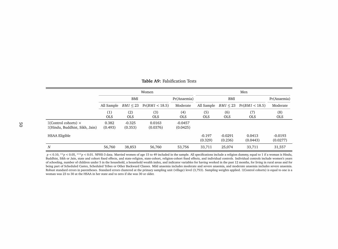
Table A9: Falsification Tests

Women Men

BMI Pr(Anaemia) BMI Pr(Anaemia)

All Sample BM I ≤ 23 Pr(BM I < 18.5) Moderate All Sample BM I ≤ 23 Pr(BM I < 18.5) Moderate

(1) (2) (3) (4) (5) (6) (7) (8)OLS OLS OLS OLS OLS OLS OLS OLS

I(Control cohorts) × 0.382 -0.325 0.0163 -0.0457I(Hindu, Buddhist, Sikh, Jain) (0.493) (0.353) (0.0376) (0.0425)

HSAA Eligible -0.197 -0.0291 0.0413 -0.0193(0.329) (0.236) (0.0443) (0.0277)

N 56,760 38,853 56,760 53,756 33,711 25,074 33,711 31,557

p < 0.10, **p < 0.05, ***p < 0.01. NFHS-3 data. Married women of age 15 to 49 included in the sample. All specifications include a religion dummy, equal to 1 if a woman is Hindu,Buddhist, Sikh or Jain, state and cohort fixed effects, and state-religion, state-cohort, religion-cohort fixed effects, and individual controls. Individual controls include women’s yearsof schooling, number of children under 5 in the household, a household wealth index, and indicator variables for having worked in the past 12 months, for living in rural areas and forbeing part of Scheduled Castes, Scheduled Tribes or Other Backward Classes. Mild anaemia includes moderate and severe anaemia, and moderate anaemia includes severe anaemia.Robust standard errors in parentheses. Standard errors clustered at the primary sampling unit (village) level (3,753). Sampling weights applied. I(Control cohorts) is equal to one is awoman was 23 to 30 at the HSAA in her state and to zero if she was 30 or older.

50

Expenditure Patterns. The improvement in women’s ability to inherit property introduced

by the HSA amendments, and the consequent increase in their lifetime unearned income, could

have an effect both on women’s bargaining power and on household expenditure behavior. In or-

der to assess whether I am indeed capturing the effect of a change in bargaining power, rather than

a change in income and wealth, I investigate how exposure to HSAA by the wife of the head of the

household affects expenditure patterns. To this aim, I use expenditure data from the 2011-2012

NSS Consumer Expenditure Survey. Firstly, I analyze the relationship between HSAA exposure

and total expenditure, and expenditures on durable and non-durable goods, respectively. If HSA

amendments determined an increase in overall expenditure, claiming existence of a causal link

between women’s intra-household bargaining power and their health would be problematic. I then

analyze the effect of exposure to HSA amendments on food expenditure shares. My motivation is

twofold. On one hand, this type of analysis may provide additional evidence of the effect of expo-

sure to the reforms on the household expenditure levels: if HSAA exposure increased household

total expenditure, we would expect the budget share of food to decrease as a consequence of the

standard view that, being a necessity, food has an income elasticity less than one. On the other

hand, it allows to test whether modeling Indian household in a unitary fashion is a sensible choice.

Rejection of the unitary model - which assumes that the household acts as a single decision unit

maximizing a common utility function - would provide support to the decision of modeling Indian

household in a collective fashion.65 Exogenous changes in distribution factors, i.e., factors affecting

bargaining power but not preferences, are frequently used in the literature to test for the pooling of

resources by household members. In the spirit of Attanasio and Lechene (2002, 2010), I investigate

the effect of HSAA exposure on food budget shares. Any significant effect would provide evidence

against the unitary model.

The empirical specification is as in equation (A1), where yirsc is the logarithm of total house-

hold i expenditure, of expenditure on non-durable goods, of expenditure on durable goods, or the

budget share devoted to food or other selected commodities, respectively. Now, HSAA Eligiblersc is

the interaction between an indicator variable equal to one if the wife of the head of the household

was 14 or younger at the time of the HSA Amendment in her state and to zero if she was 23 or

older, and an indicator variable for being Hindu, Buddhist, Sikh or Jain. X ′irsc is a vector of controls

for household i, of religion r, living in state s, with the wife of the head of the household born in

year c. As standard in the literature, when looking at the effect of HSAA exposure on food budget

shares, I condition the model on the logarithm of total expenditure. Due to data availability, I

only estimate an intent-to-treat effect. Standard errors are clustered at the first sampling unit level

(2001 Census villages in rural areas and 2007-2012 Urban Frame Survey blocks in urban areas).

Table A10 reports the estimation results of the effect of HSAA eligibility of the wife of the head of

household on expenditure patterns. All specifications include individual controls and religion-state,

state-cohort and cohort-religion fixed effects. Column 1 to 3 show the estimated coefficients of the

65There is a large consensus in the literature that a model should account for household members having different preferences and for theintra-household distribution of powers. However, evidence against the unitary model does not automatically imply evidence in favor of thecollective model.

51

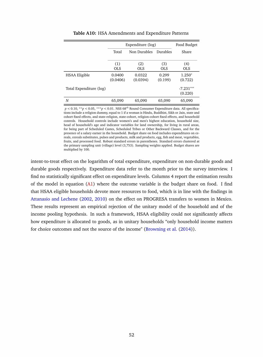
Table A10: HSA Amendments and Expenditure Patterns

Expenditure (log) Food Budget

Total Non Durables Durables Share

(1) (2) (3) (4)OLS OLS OLS OLS

HSAA Eligible 0.0400 0.0322 0.299 1.250∗

(0.0406) (0.0394) (0.199) (0.722)

Total Expenditure (log) -7.231∗∗∗

(0.220)

N 65,090 65,090 65,090 65,090

p < 0.10, **p < 0.05, ***p < 0.01. NSS 68th Round Consumer Expenditure data. All specifica-tions include a religion dummy, equal to 1 if a woman is Hindu, Buddhist, Sikh or Jain, state andcohort fixed effects, and state-religion, state-cohort, religion-cohort fixed effects, and householdcontrols. Household controls include women’s and men’s highest education, household size,head of household’s age and indicator variables for land ownership, for living in rural areas,for being part of Scheduled Castes, Scheduled Tribes or Other Backward Classes, and for thepresence of a salary earner in the household. Budget share on food includes expenditures on ce-reals, cereals substitutes, pulses and products, milk and products, egg, fish and meat, vegetables,fruits, and processed food. Robust standard errors in parentheses. Standard errors clustered atthe primary sampling unit (village) level (3,753). Sampling weights applied. Budget shares aremultiplied by 100.

intent-to-treat effect on the logarithm of total expenditure, expenditure on non-durable goods and

durable goods respectively. Expenditure data refer to the month prior to the survey interview. I

find no statistically significant effect on expenditure levels. Columns 4 report the estimation results

of the model in equation (A1) where the outcome variable is the budget share on food. I find

that HSAA eligible households devote more resources to food, which is in line with the findings in

Attanasio and Lechene (2002, 2010) on the effect on PROGRESA transfers to women in Mexico.

These results represent an empirical rejection of the unitary model of the household and of the

income pooling hypothesis. In such a framework, HSAA eligibility could not significantly affects

how expenditure is allocated to goods, as in unitary households “only household income matters

for choice outcomes and not the source of the income" (Browning et al. (2014)).

52

A.4 A Fully Specified Collective Model of Indian Households

The empirical estimation of resource shares assumes Engel curves for the private assignable goods

to be linear in ln y and requires resource shares to be independent of y . However, it does not invoke

restrictions on other goods’ demand functions. I here provide a fully specified household model that

delivers linearity of Engel curves and resource shares that are independent of y . h= (h1, ...,hK) is

the vector of observed quantities of goods purchased by each household, while x t = (x1t ..., xK

t ) is

the vector of unobserved quantities of goods consumed by an individual of type t = f , m, c.

Assume each household member of type t, t = f , m, c, has utility given by Muellbauer’s Price

Independent Generalized Logarithmic (Piglog) model. In this framework, the indirect utility func-

tions can be written as follows:

v��

y

Gt(p)

��

+ Ft(p) = ln�

ln�

y

Gt(p)

��

+ Ft(p) (A3)

with Ft(p) = pt exp (−a′ ln p), for some constant vector a with elements ak summing to one. Let p

contain the prices of all goods except the prices of the private assignable goods for adult females,

adult males and children, p f , pm, pc. The assumption of assigning the same utility function to

members of the same type is data driven and constrained by the number of different assignable

goods that can be observed. For simplicity, consider the transformationψt(v+Ft , p) = exp (v+ Ft),

which not depending upon p makes the individual Engel curves for all goods to be the same as

those of the private assignable goods. While this assumption is not invoked in the estimation

of the system of Engel curves in equation 6, it simplifies the derivation of the full model. Let

Gt(p) = Gt(pt , p), which makes explicit the assumption that the, for example, the price pm of the

good that is assignable to the father does not appear in the woman’s utility function, and hence

does not appear in G f (p f , p).

The indirect utility function for individuals of type t is given by:

Vt = ln�

y

Gt(pt , p)

�

exp (pt exp(−a′ ln p)) (A4)

Each household utility function can be characterized as a Bergson-Samuelson social welfare

function, U , featuring the relative weights of the utility functions of its members:

U(U f , Um, Uc, p/y) =∑

t∈{ f ,m,c}

µt(p/y)[Ut + ξt(p/y)] (A5)

where µt(p/y) is the Pareto weight and ξt(p/y) are externality functions capturing the extent to

which one’s consumption affect the other member of the household. µt and ξt must be homoge-

neous of degree zero, so that µt(p/y) = µt(p) and ξt(p/y) = ξt(p) (Dunbar et al. (2013)). Pareto

weights are traditionally interpreted as measures of intra-household bargaining power. The larger

the value of µt , the greater is the weight that type t members’ preferences receive in the household

program.

53

Let A be the matrix defining the extent of joint consumption in each household and character-

izing the consumption technology function. In other words, the consumption technology function

converts purchased quantities by the household, h, in private good equivalents, x . While the general

framework allows for a non-diagonal A, I here assume it to be diagonal. Non-zero off diagonal ele-

ments of A may arise when the extent to which one good is shared depends upon other goods, e.g.„

if leisure time is a consumption good, then the degree to which a motorcycle use is shared may

depend on the time involved. A private good is defined as a good with its corresponding diagonal

element of A equal to 1, and all off-diagonal elements in that row or column are equal to 0. Each

household solves the following program:

maxx f ,xm,xc ,h

ξ(p) +∑

t∈{ f ,m,c}

µt(p)Ut subject to h= A(F x f +M xm+ C xc)

y = h′p (A6)

where ξ(p) =∑

t∈{ f ,m,c}µt(p)ξt(p) and F , M and C are the total number of adult women, adult

men and children in the household, respectively. Let λt the resource share for each individuals of

type t, such that λt =∑

kAk pk x tk

y.

This program can be decomposed in two steps: 1) the optimal allocation of resources across

members and 2) the individual maximization of their own utility function. This results follows

directly from the second welfare theorem, as any Pareto efficient allocation can be implemented as

an equilibrium of this economy, possibly after lump sum transfers between members. Conditional

on knowing λt , each household member chooses x t as the bundle maximizing Ut subject to the

Lindahl type shadow budget constraint∑

k Akpk x kt = λt y . Substituting the indirect utility functions

Vt(A′p,λt y) in the program above simplifies the optimization problem to the choice of optimal

resource shares subject to the constraint that total resources shares must sum to one. The household

program can be therefore written as:

maxλ f ,λm,λc

ξ(p)+∑

t∈{ f ,m,c}

µt(p)Vt(A′p,λt(p/y)y) subject to Fλ f (p/y)+Mλm(p/y)+Cλc(p/y) = 1

(A7)

and, given the functional form assumptions discussed above, as:

maxλ f ,λm,λc

ξ+∑

t∈{ f ,m,c}

µt

�

lnλt y

Gt

�

subject to Λ f +Λm+Λc = 1 (A8)

with µt(p) = µt(p)exp (At pt exp(−a′(ln p+ ln A))). The first order conditions of the Lagrangean

are as follows:

µ f

Λ f= µm

Λm= µc

Λc= ν

Λ f +Λm+Λc = 1(A9)

with ν being the Lagrange multiplier. Explicit formulas for resource shares can be derived from the

54

solution of the system of equations above. For individuals of type t = f , m, c, the overall resource

shares are defined as

Λt(p/y) = Λt(p) =µt(p)

∑

t∈{ f ,m,c} µt(p)(A10)

Assuming equal sharing among individuals of the same type, individual resources shares for type t

household members are defined as

λt(p) =µt(p)/T

∑

t∈{ f ,m,c} µt(p)(A11)

with T = F, M , C . As required for identification, these explicit formulas for the resource shares do

not depend on y .

Each household member chooses x t as the bundle maximizing Ut subject to the constraint∑

k Akpk x kt = λt y . The individuals’ demand function for good k, k = 1, ..., K , can be obtained by

Roy’s identity to equation (A4), with prices equal to Apk and income equal to λt y:

x kt (λt y, A′p) =−

∂ Vt(λt y, A′p)/∂ Apk

∂ Vt(λt y, A′p)/∂ λt y

= λt y

�

∂ Gt

∂ Apk

1

Gt−∂ (Apt exp (−a′ ln p))

∂ Apk

�

ln(λt y)− ln Gt�

�

=∂ Gt

∂ Apk

λt y

Gt−∂ (Apt exp (−a′ ln p))

∂ Apk

�

ln(λt y)− ln Gt�

λt y (A12)

for each good k and any individual t. Using the consumption technology function, the household

demand function for a generic good k, as fraction of the total expenditure, is then defined as:

hk(p, y)y

= Ak

∑

t∈{ f ,m,c}

T x kt (λt(p)y, A′p)

y(A13)

Equation (A12) can be rewritten as:

x kt (λt y, A′p) = λt yαk

t +λt yβ kt ln(λt y) (A14)

The overall demand of good k from individuals of type t generated from the solution of the decen-

tralized optimization problems is given by:

T x kt (λt(p)y, A′p) = Λt yαk

t +Λt yβ kt (ln y + lnΛt − ln T ) (A15)

and the corresponding budget share is:

T x kt (λt(p)y, A′p)

y= Λt(p)α

kt (p) +Λt(p)β

kt (p)(ln y + lnΛt(p)− ln T ) (A16)

where T = F, M , C , t = f , m, c, and Λt = Tλt .

55

An Engel curve represents the relationship between a budget share and total expenditure, hold-

ing prices constant. The Engel curve for a generic good k, under the explicit assumptions made

above, takes the following form

hk(y)y= Ak

∑

t∈{ f ,m,c}

[Λtαkt +Λtβ

kt (ln y + lnΛt − ln T )] (A17)

and for private assignable goods it simplifies to

Wt(y) =ht(y)

y= Λtαt +Λtβt(ln y + lnΛt − ln T ) (A18)

56

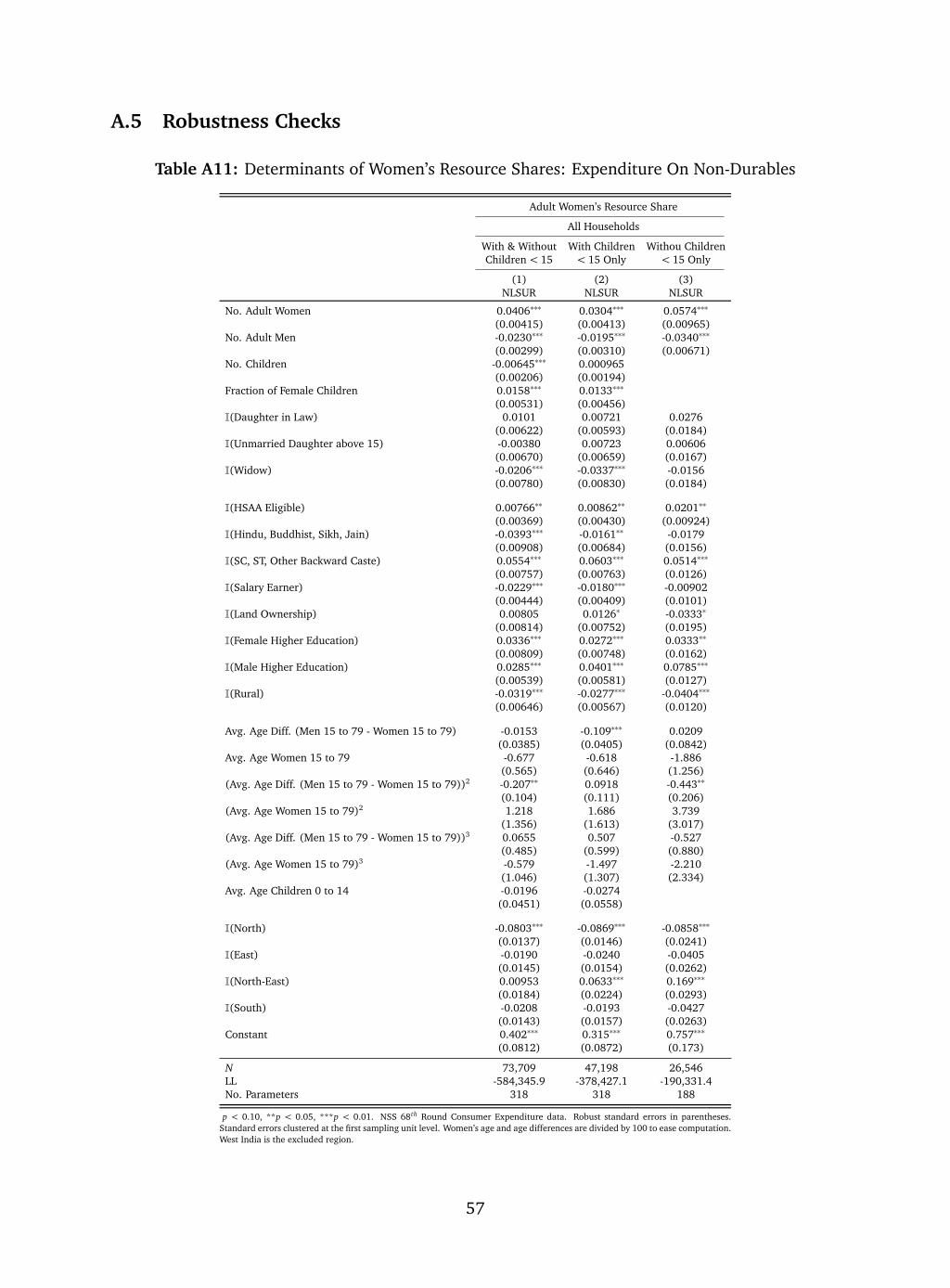
A.5 Robustness Checks

Table A11: Determinants of Women’s Resource Shares: Expenditure On Non-Durables

Adult Women’s Resource Share

All Households

With & Without With Children Withou ChildrenChildren < 15 < 15 Only < 15 Only

(1) (2) (3)NLSUR NLSUR NLSUR

No. Adult Women 0.0406∗∗∗ 0.0304∗∗∗ 0.0574∗∗∗

(0.00415) (0.00413) (0.00965)No. Adult Men -0.0230∗∗∗ -0.0195∗∗∗ -0.0340∗∗∗

(0.00299) (0.00310) (0.00671)No. Children -0.00645∗∗∗ 0.000965

(0.00206) (0.00194)Fraction of Female Children 0.0158∗∗∗ 0.0133∗∗∗

(0.00531) (0.00456)I(Daughter in Law) 0.0101 0.00721 0.0276

(0.00622) (0.00593) (0.0184)I(Unmarried Daughter above 15) -0.00380 0.00723 0.00606

(0.00670) (0.00659) (0.0167)I(Widow) -0.0206∗∗∗ -0.0337∗∗∗ -0.0156

(0.00780) (0.00830) (0.0184)

I(HSAA Eligible) 0.00766∗∗ 0.00862∗∗ 0.0201∗∗

(0.00369) (0.00430) (0.00924)I(Hindu, Buddhist, Sikh, Jain) -0.0393∗∗∗ -0.0161∗∗ -0.0179

(0.00908) (0.00684) (0.0156)I(SC, ST, Other Backward Caste) 0.0554∗∗∗ 0.0603∗∗∗ 0.0514∗∗∗

(0.00757) (0.00763) (0.0126)I(Salary Earner) -0.0229∗∗∗ -0.0180∗∗∗ -0.00902

(0.00444) (0.00409) (0.0101)I(Land Ownership) 0.00805 0.0126∗ -0.0333∗

(0.00814) (0.00752) (0.0195)I(Female Higher Education) 0.0336∗∗∗ 0.0272∗∗∗ 0.0333∗∗

(0.00809) (0.00748) (0.0162)I(Male Higher Education) 0.0285∗∗∗ 0.0401∗∗∗ 0.0785∗∗∗

(0.00539) (0.00581) (0.0127)I(Rural) -0.0319∗∗∗ -0.0277∗∗∗ -0.0404∗∗∗

(0.00646) (0.00567) (0.0120)

Avg. Age Diff. (Men 15 to 79 - Women 15 to 79) -0.0153 -0.109∗∗∗ 0.0209(0.0385) (0.0405) (0.0842)

Avg. Age Women 15 to 79 -0.677 -0.618 -1.886(0.565) (0.646) (1.256)

(Avg. Age Diff. (Men 15 to 79 - Women 15 to 79))2 -0.207∗∗ 0.0918 -0.443∗∗

(0.104) (0.111) (0.206)(Avg. Age Women 15 to 79)2 1.218 1.686 3.739

(1.356) (1.613) (3.017)(Avg. Age Diff. (Men 15 to 79 - Women 15 to 79))3 0.0655 0.507 -0.527

(0.485) (0.599) (0.880)(Avg. Age Women 15 to 79)3 -0.579 -1.497 -2.210

(1.046) (1.307) (2.334)Avg. Age Children 0 to 14 -0.0196 -0.0274

(0.0451) (0.0558)

I(North) -0.0803∗∗∗ -0.0869∗∗∗ -0.0858∗∗∗

(0.0137) (0.0146) (0.0241)I(East) -0.0190 -0.0240 -0.0405

(0.0145) (0.0154) (0.0262)I(North-East) 0.00953 0.0633∗∗∗ 0.169∗∗∗

(0.0184) (0.0224) (0.0293)I(South) -0.0208 -0.0193 -0.0427

(0.0143) (0.0157) (0.0263)Constant 0.402∗∗∗ 0.315∗∗∗ 0.757∗∗∗

(0.0812) (0.0872) (0.173)

N 73,709 47,198 26,546LL -584,345.9 -378,427.1 -190,331.4No. Parameters 318 318 188

p < 0.10, **p < 0.05, ***p < 0.01. NSS 68th Round Consumer Expenditure data. Robust standard errors in parentheses.Standard errors clustered at the first sampling unit level. Women’s age and age differences are divided by 100 to ease computation.West India is the excluded region.

57

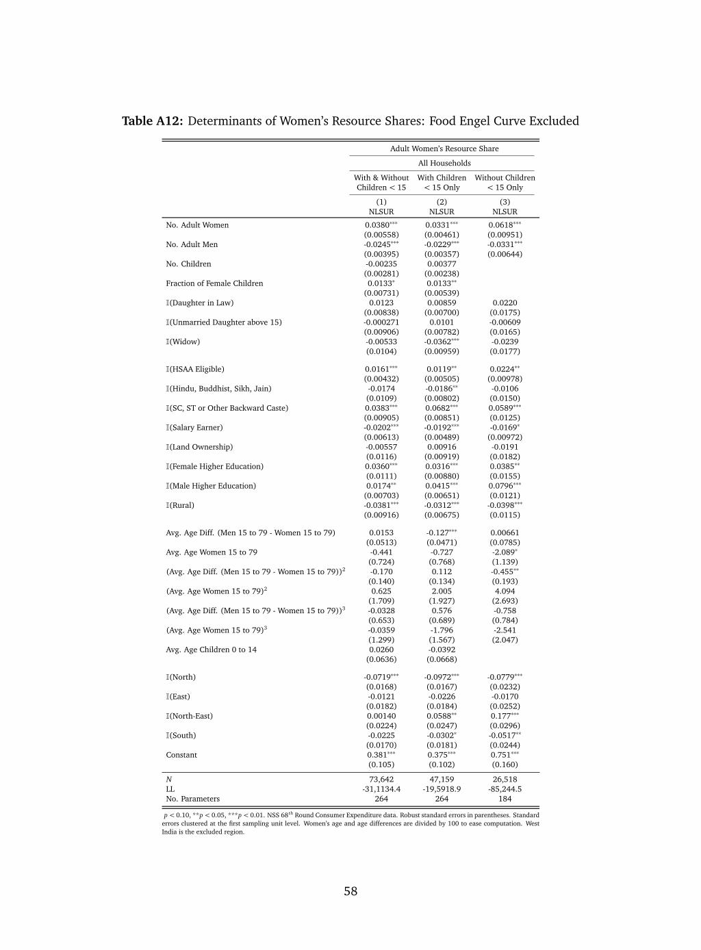
Table A12: Determinants of Women’s Resource Shares: Food Engel Curve Excluded

Adult Women’s Resource Share

All Households

With & Without With Children Without ChildrenChildren < 15 < 15 Only < 15 Only

(1) (2) (3)NLSUR NLSUR NLSUR

No. Adult Women 0.0380∗∗∗ 0.0331∗∗∗ 0.0618∗∗∗

(0.00558) (0.00461) (0.00951)No. Adult Men -0.0245∗∗∗ -0.0229∗∗∗ -0.0331∗∗∗

(0.00395) (0.00357) (0.00644)No. Children -0.00235 0.00377

(0.00281) (0.00238)Fraction of Female Children 0.0133∗ 0.0133∗∗

(0.00731) (0.00539)I(Daughter in Law) 0.0123 0.00859 0.0220

(0.00838) (0.00700) (0.0175)I(Unmarried Daughter above 15) -0.000271 0.0101 -0.00609

(0.00906) (0.00782) (0.0165)I(Widow) -0.00533 -0.0362∗∗∗ -0.0239

(0.0104) (0.00959) (0.0177)

I(HSAA Eligible) 0.0161∗∗∗ 0.0119∗∗ 0.0224∗∗

(0.00432) (0.00505) (0.00978)I(Hindu, Buddhist, Sikh, Jain) -0.0174 -0.0186∗∗ -0.0106

(0.0109) (0.00802) (0.0150)I(SC, ST or Other Backward Caste) 0.0383∗∗∗ 0.0682∗∗∗ 0.0589∗∗∗

(0.00905) (0.00851) (0.0125)I(Salary Earner) -0.0202∗∗∗ -0.0192∗∗∗ -0.0169∗

(0.00613) (0.00489) (0.00972)I(Land Ownership) -0.00557 0.00916 -0.0191

(0.0116) (0.00919) (0.0182)I(Female Higher Education) 0.0360∗∗∗ 0.0316∗∗∗ 0.0385∗∗

(0.0111) (0.00880) (0.0155)I(Male Higher Education) 0.0174∗∗ 0.0415∗∗∗ 0.0796∗∗∗

(0.00703) (0.00651) (0.0121)I(Rural) -0.0381∗∗∗ -0.0312∗∗∗ -0.0398∗∗∗

(0.00916) (0.00675) (0.0115)

Avg. Age Diff. (Men 15 to 79 - Women 15 to 79) 0.0153 -0.127∗∗∗ 0.00661(0.0513) (0.0471) (0.0785)

Avg. Age Women 15 to 79 -0.441 -0.727 -2.089∗

(0.724) (0.768) (1.139)(Avg. Age Diff. (Men 15 to 79 - Women 15 to 79))2 -0.170 0.112 -0.455∗∗

(0.140) (0.134) (0.193)(Avg. Age Women 15 to 79)2 0.625 2.005 4.094

(1.709) (1.927) (2.693)(Avg. Age Diff. (Men 15 to 79 - Women 15 to 79))3 -0.0328 0.576 -0.758

(0.653) (0.689) (0.784)(Avg. Age Women 15 to 79)3 -0.0359 -1.796 -2.541

(1.299) (1.567) (2.047)Avg. Age Children 0 to 14 0.0260 -0.0392

(0.0636) (0.0668)

I(North) -0.0719∗∗∗ -0.0972∗∗∗ -0.0779∗∗∗

(0.0168) (0.0167) (0.0232)I(East) -0.0121 -0.0226 -0.0170

(0.0182) (0.0184) (0.0252)I(North-East) 0.00140 0.0588∗∗ 0.177∗∗∗

(0.0224) (0.0247) (0.0296)I(South) -0.0225 -0.0302∗ -0.0517∗∗

(0.0170) (0.0181) (0.0244)Constant 0.381∗∗∗ 0.375∗∗∗ 0.751∗∗∗

(0.105) (0.102) (0.160)

N 73,642 47,159 26,518LL -31,1134.4 -19,5918.9 -85,244.5No. Parameters 264 264 184

p < 0.10, **p < 0.05, ***p < 0.01. NSS 68th Round Consumer Expenditure data. Robust standard errors in parentheses. Standarderrors clustered at the first sampling unit level. Women’s age and age differences are divided by 100 to ease computation. WestIndia is the excluded region.

58

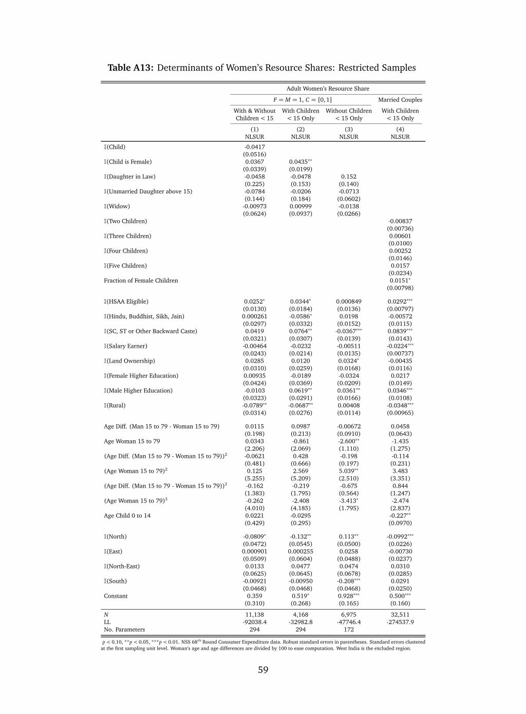
Table A13: Determinants of Women’s Resource Shares: Restricted Samples

Adult Women’s Resource Share

F = M = 1, C = {0,1} Married Couples

With & Without With Children Without Children With ChildrenChildren < 15 < 15 Only < 15 Only < 15 Only

(1) (2) (3) (4)NLSUR NLSUR NLSUR NLSUR

I(Child) -0.0417(0.0516)

I(Child is Female) 0.0367 0.0435∗∗

(0.0339) (0.0199)I(Daughter in Law) -0.0458 -0.0478 0.152

(0.225) (0.153) (0.140)I(Unmarried Daughter above 15) -0.0784 -0.0206 -0.0713

(0.144) (0.184) (0.0602)I(Widow) -0.00973 0.00999 -0.0138

(0.0624) (0.0937) (0.0266)I(Two Children) -0.00837

(0.00736)I(Three Children) 0.00601

(0.0100)I(Four Children) 0.00252

(0.0146)I(Five Children) 0.0157

(0.0234)Fraction of Female Children 0.0151∗

(0.00798)

I(HSAA Eligible) 0.0252∗ 0.0344∗ 0.000849 0.0292∗∗∗

(0.0130) (0.0184) (0.0136) (0.00797)I(Hindu, Buddhist, Sikh, Jain) 0.000261 -0.0586∗ 0.0198 -0.00572

(0.0297) (0.0332) (0.0152) (0.0115)I(SC, ST or Other Backward Caste) 0.0419 0.0764∗∗ -0.0367∗∗∗ 0.0839∗∗∗

(0.0321) (0.0307) (0.0139) (0.0143)I(Salary Earner) -0.00464 -0.0232 -0.00511 -0.0224∗∗∗

(0.0243) (0.0214) (0.0135) (0.00737)I(Land Ownership) 0.0285 0.0120 0.0324∗ -0.00435

(0.0310) (0.0259) (0.0168) (0.0116)I(Female Higher Education) 0.00935 -0.0189 -0.0324 0.0217

(0.0424) (0.0369) (0.0209) (0.0149)I(Male Higher Education) -0.0103 0.0619∗∗ 0.0361∗∗ 0.0346∗∗∗

(0.0323) (0.0291) (0.0166) (0.0108)I(Rural) -0.0789∗∗ -0.0687∗∗ 0.00408 -0.0348∗∗∗

(0.0314) (0.0276) (0.0114) (0.00965)

Age Diff. (Man 15 to 79 - Woman 15 to 79) 0.0115 0.0987 -0.00672 0.0458(0.198) (0.213) (0.0910) (0.0643)

Age Woman 15 to 79 0.0343 -0.861 -2.600∗∗ -1.435(2.206) (2.069) (1.110) (1.275)

(Age Diff. (Man 15 to 79 - Woman 15 to 79))2 -0.0621 0.428 -0.198 -0.114(0.481) (0.666) (0.197) (0.231)

(Age Woman 15 to 79)2 0.125 2.569 5.039∗∗ 3.483(5.255) (5.209) (2.510) (3.351)

(Age Diff. (Man 15 to 79 - Woman 15 to 79))3 -0.162 -0.219 -0.675 0.844(1.383) (1.795) (0.564) (1.247)

(Age Woman 15 to 79)3 -0.262 -2.408 -3.413∗ -2.474(4.010) (4.185) (1.795) (2.837)

Age Child 0 to 14 0.0221 -0.0295 -0.227∗∗

(0.429) (0.295) (0.0970)

I(North) -0.0809∗ -0.132∗∗ 0.113∗∗ -0.0992∗∗∗

(0.0472) (0.0545) (0.0500) (0.0226)I(East) 0.000901 0.000255 0.0258 -0.00730

(0.0509) (0.0604) (0.0488) (0.0237)I(North-East) 0.0133 0.0477 0.0474 0.0310

(0.0625) (0.0645) (0.0678) (0.0285)I(South) -0.00921 -0.00950 -0.208∗∗∗ 0.0291

(0.0468) (0.0468) (0.0468) (0.0250)Constant 0.359 0.519∗ 0.928∗∗∗ 0.500∗∗∗

(0.310) (0.268) (0.165) (0.160)

N 11,138 4,168 6,975 32,511LL -92038.4 -32982.8 -47746.4 -274537.9No. Parameters 294 294 172

p < 0.10, **p < 0.05, ***p < 0.01. NSS 68th Round Consumer Expenditure data. Robust standard errors in parentheses. Standard errors clusteredat the first sampling unit level. Woman’s age and age differences are divided by 100 to ease computation. West India is the excluded region.

59

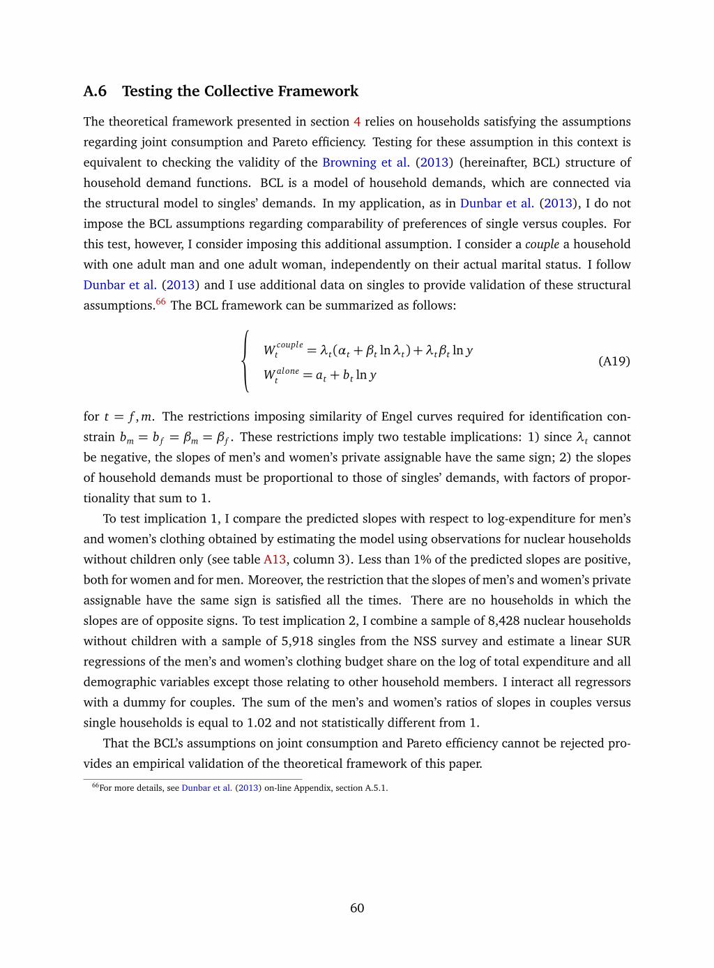
A.6 Testing the Collective Framework

The theoretical framework presented in section 4 relies on households satisfying the assumptions

regarding joint consumption and Pareto efficiency. Testing for these assumption in this context is

equivalent to checking the validity of the Browning et al. (2013) (hereinafter, BCL) structure of

household demand functions. BCL is a model of household demands, which are connected via

the structural model to singles’ demands. In my application, as in Dunbar et al. (2013), I do not

impose the BCL assumptions regarding comparability of preferences of single versus couples. For

this test, however, I consider imposing this additional assumption. I consider a couple a household

with one adult man and one adult woman, independently on their actual marital status. I follow

Dunbar et al. (2013) and I use additional data on singles to provide validation of these structural

assumptions.66 The BCL framework can be summarized as follows:

W couplet = λt(αt + βt lnλt) +λtβt ln y

W alonet = at + bt ln y

(A19)

for t = f , m. The restrictions imposing similarity of Engel curves required for identification con-

strain bm = b f = βm = β f . These restrictions imply two testable implications: 1) since λt cannot

be negative, the slopes of men’s and women’s private assignable have the same sign; 2) the slopes

of household demands must be proportional to those of singles’ demands, with factors of propor-

tionality that sum to 1.

To test implication 1, I compare the predicted slopes with respect to log-expenditure for men’s

and women’s clothing obtained by estimating the model using observations for nuclear households

without children only (see table A13, column 3). Less than 1% of the predicted slopes are positive,

both for women and for men. Moreover, the restriction that the slopes of men’s and women’s private

assignable have the same sign is satisfied all the times. There are no households in which the

slopes are of opposite signs. To test implication 2, I combine a sample of 8,428 nuclear households

without children with a sample of 5,918 singles from the NSS survey and estimate a linear SUR

regressions of the men’s and women’s clothing budget share on the log of total expenditure and all

demographic variables except those relating to other household members. I interact all regressors

with a dummy for couples. The sum of the men’s and women’s ratios of slopes in couples versus

single households is equal to 1.02 and not statistically different from 1.

That the BCL’s assumptions on joint consumption and Pareto efficiency cannot be rejected pro-

vides an empirical validation of the theoretical framework of this paper.

66For more details, see Dunbar et al. (2013) on-line Appendix, section A.5.1.

60

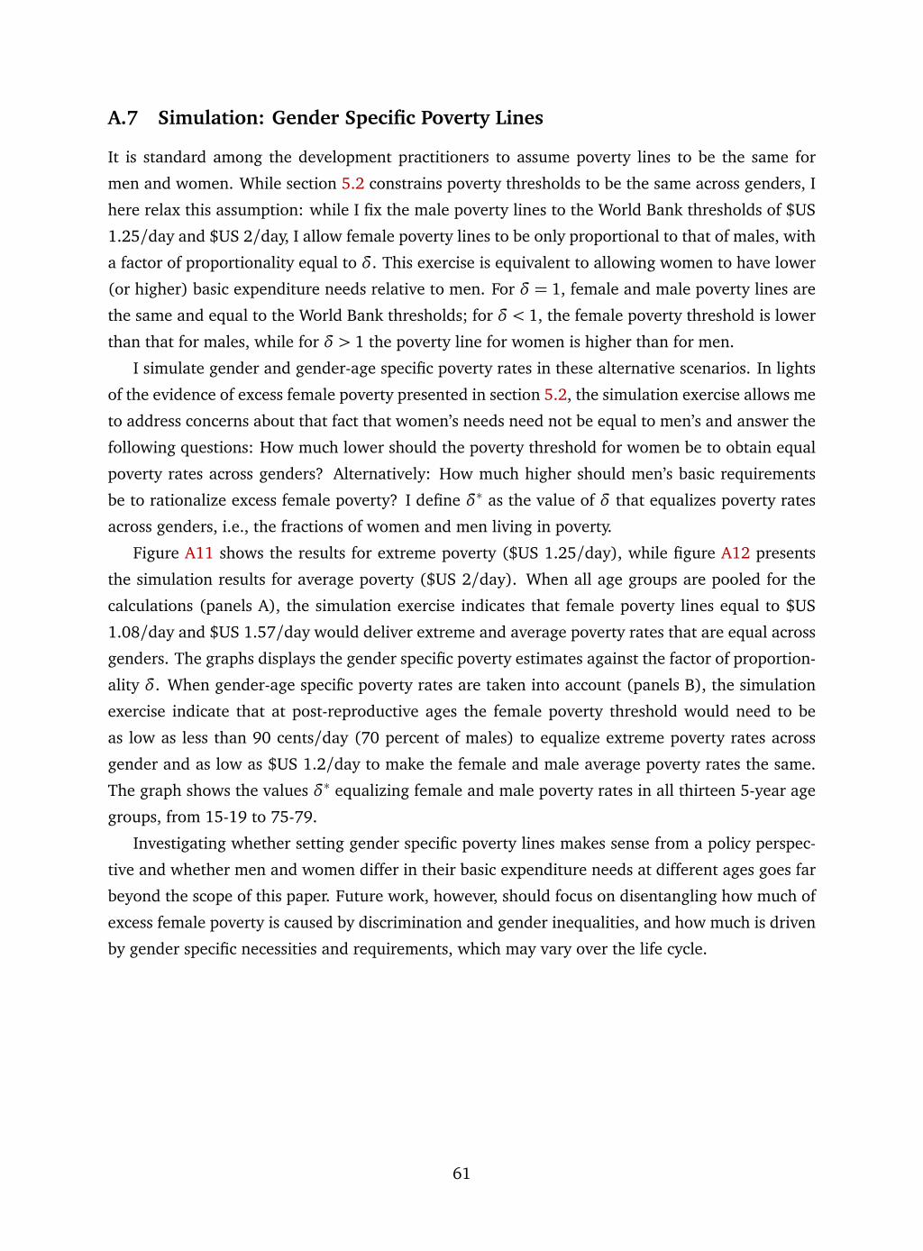
A.7 Simulation: Gender Specific Poverty Lines

It is standard among the development practitioners to assume poverty lines to be the same for

men and women. While section 5.2 constrains poverty thresholds to be the same across genders, I

here relax this assumption: while I fix the male poverty lines to the World Bank thresholds of $US

1.25/day and $US 2/day, I allow female poverty lines to be only proportional to that of males, with

a factor of proportionality equal to δ. This exercise is equivalent to allowing women to have lower

(or higher) basic expenditure needs relative to men. For δ = 1, female and male poverty lines are

the same and equal to the World Bank thresholds; for δ < 1, the female poverty threshold is lower

than that for males, while for δ > 1 the poverty line for women is higher than for men.

I simulate gender and gender-age specific poverty rates in these alternative scenarios. In lights

of the evidence of excess female poverty presented in section 5.2, the simulation exercise allows me

to address concerns about that fact that women’s needs need not be equal to men’s and answer the

following questions: How much lower should the poverty threshold for women be to obtain equal

poverty rates across genders? Alternatively: How much higher should men’s basic requirements

be to rationalize excess female poverty? I define δ∗ as the value of δ that equalizes poverty rates

across genders, i.e., the fractions of women and men living in poverty.

Figure A11 shows the results for extreme poverty ($US 1.25/day), while figure A12 presents

the simulation results for average poverty ($US 2/day). When all age groups are pooled for the

calculations (panels A), the simulation exercise indicates that female poverty lines equal to $US

1.08/day and $US 1.57/day would deliver extreme and average poverty rates that are equal across

genders. The graphs displays the gender specific poverty estimates against the factor of proportion-

ality δ. When gender-age specific poverty rates are taken into account (panels B), the simulation

exercise indicate that at post-reproductive ages the female poverty threshold would need to be

as low as less than 90 cents/day (70 percent of males) to equalize extreme poverty rates across

gender and as low as $US 1.2/day to make the female and male average poverty rates the same.

The graph shows the values δ∗ equalizing female and male poverty rates in all thirteen 5-year age

groups, from 15-19 to 75-79.

Investigating whether setting gender specific poverty lines makes sense from a policy perspec-

tive and whether men and women differ in their basic expenditure needs at different ages goes far

beyond the scope of this paper. Future work, however, should focus on disentangling how much of

excess female poverty is caused by discrimination and gender inequalities, and how much is driven

by gender specific necessities and requirements, which may vary over the life cycle.

61

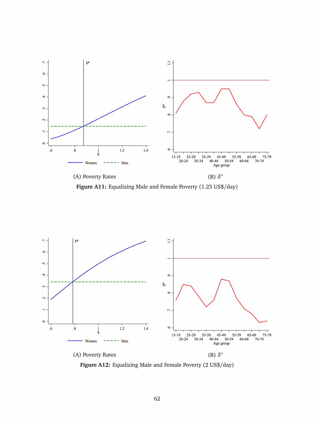
(A) Poverty Rates (B) δ∗

Figure A11: Equalizing Male and Female Poverty (1.25 US$/day)

(A) Poverty Rates (B) δ∗

Figure A12: Equalizing Male and Female Poverty (2 US$/day)

62