R u t c o r

Research

R e p o r t

RUTCOR

Rutgers Center for

Operations Research

Rutgers University

640 Bartholomew Road

Piscataway, New Jersey

08854-8003

Telephone: 732-445-3804

Telefax: 732-445-5472

Email: rrr@rutcor.rutgers.edu

http://rutcor.rutgers.edu/∼rrr

Why Chess and Backgammon canbe solved in pure positionaluniformly optimal strategies

Endre Borosa Vladimir Gurvichb

RRR 21-2009, September 2009

aRUTCOR, Rutgers University, 640 Bartholomew Road, Piscataway NJ08854-8003; (boros@rutcor.rutgers.edu)

bRUTCOR, Rutgers University, 640 Bartholomew Road, Piscataway NJ08854-8003; (gurvich@rutcor.rutgers.edu). The second author is thankful forpartial support to Center for Algorithmic Game Theory and Research Foun-dation, University of Aarhus; School of Information Science and Technology,University of Tokyo; Lab. of Optimization and Combinatorics, UniversityPierre and Marie Curie, Paris VI.

Rutcor Research Report

RRR 21-2009, September 2009

Why Chess and Backgammon can be solvedin pure positional uniformly optimal

strategies

Endre Boros, Vladimir Gurvich

Abstract. We study existence of (subgame perfect) Nash equilibria (NE) in purepositional strategies in finite positional n-person games with perfect information andterminal payoffs. However, these games may have moves of chance and cycles. Yet,we assume that All Infinite Plays Form One Outcome a∞, in addition to the set ofTerminal outcomes VT . This assumption will be called the AIPFOOT condition.For example, Chess or Backgammon are AIPFOOT games, since each infinite play isa draw, by definition. All terminals and a∞ are ranked arbitrarily by the n players.

It is well-known that in each finite acyclic positional game, a subgame perfect NEexists and it can be easily found by backward induction, suggested by Kuhn andGale in early 50s. In contrast, there is a two-person game with only one cycle, onerandom position, and without NE in pure positional strategies. In 1912, Zermeloproved that each two-person zero-sum AIPFOOT game without random moves (forexample, Chess) has a saddle point in pure strategies. Yet, there are cycles in Chess.Zermelo’s result can be extended in two directions:

(i) Each two-person (not necessarily zero-sum) AIPFOOT game without randommoves has a (not necessarily subgame perfect) NE in pure positional strategies;although, the similar statement remains a conjecture for the n-person case.

(ii) Each two-person zero-sum AIPFOOT game (which might have random moves)has saddle point in pure positional uniformly optimal strategies.

Surprisingly, to prove (ii), it appears convenient to treat such a game (for example,Backgammon or even Chess) as a stochastic game with perfect information.

Key words: Backgammon, Chess, pure strategies, positional strategies, Nahh equi-librium, ergodic, subgame perfect, uniformly optimal, stochastic game, perfect in-formation, position, random move, Zermelo, Kuhn, Gale

Acknowledgements: This research was supported by DIMACS, Center for DiscreteMathematics and Theoretical Computer Science

Page 2 RRR 21-2009

1 Introduction

We study existence of (subgame perfect) Nash equilibria in pure positional strategies infinite positional n-person games with perfect information and terminal payoffs. The gamesunder consideration may have moves of chance and cycles. Yet, we assume that All InfinitePlays Form One Outcome a∞, in addition to the Terminal outcomes VT = {a1, . . . , ap}; thisassumption will be called the AIPFOOT condition. For example, Chess or Backgammonare AIPFOOT games, since the set of positions is finite and every infinite play is a draw,by definition. In general, a∞ and all terminal positions form the set of outcomes, A =VT ∪ {a∞} = {a1, . . . , ap, a∞}, which are ranked arbitrarily by n players I = {1, . . . , n}.

In 1950, Nash introduced his concept of equilibrium [33, 34] (so called Nash equilibrium;NE, for short) . In the same year, Kuhn [28, 29] suggested a construction showing that asubgame perfect NE exists in every acyclic game, which might have moves of chance butcannot have cycles. Accurately speaking, Kuhn restricted his analysis to trees, yet, themethod, so-called backward induction, can be easily extended to the acyclic digraphs; see,for example, Section 2.5. Thus, the acyclic case is simple. In this paper we focus on theAIPFOOT games, which naturally may have cycles.

In Section 3.3 we shall extend the backward induction procedure to the two-person zero-sum AIPFOOT games without random moves, like Chess, and prove existence of a saddlepoint in pure positional uniformly optimal strategies.

Furthermore, every n-person AIPFOOT game without random moves, has a NE in purestationary (but not necessarily positional) strategies. The proof is simple; see, for example,Section 2.11. The graph G of such a game can be ”unfolded” as a finite tree T whose verticesare the debuts of the original game. In particular, a position of G might appear in T severaltimes. Then, one can apply backward induction to T , to obtain a subgame perfect NE.However, this NE, ”projected” onto the original game, might not be subgame perfect and,although the corresponding strategies are pure, they might not be positional; indeed, byconstruction, a move in a position v in G depends not only on v but also on the debut thatbrought the play to v, that is, on the previous positions and moves.

The lack of these two important properties is not a fault of the above algorithm. Subgameperfect NE in pure positional strategies may just fail to exist, in presence of cycles.

In particular, a unique NE in pure positional strategies is not subgame perfect in a verysimple two-person game, with only one cycle and two non-terminal positions, none of whichis random; see Example 1. Furthermore, there are games with only one cycle, one positionof chance, and no NE in pure positional strategies; see Examples 2 and 3.

Yet, by the so-called Folk Theorem, a (not necessarily subgame perfect) NE in pure (butnot necessarily positional) strategies exists in every n-person AIPFOOT game, which mighthave both cycles and positions of chance; see Sections 2.11.

In 1912, Zermelo proved that each two-person zero-sum AIPFOOT game without movesof chance has a saddle point in pure strategies [37]. He considered Chess as an example (letus notice that there are cycles in Chess). Zermelo’s result can be extended in two ways:

RRR 21-2009 Page 3

(i) Each two-person AIPFOOT game without moves of chance has a (not necessarilysubgame perfect) NE in pure positional strategies.

(ii) Each two-person zero-sum AIPFOOT game has a subgame perfect saddle point in purepositional uniformly optimal strategies.

Yet, it remains an open question whether (i) can be extended to the n-person case; seeSection 2.7. Let us also note that (ii) is applicable to games with random moves and cycles;for example, to Backgammon.

Remark 1 By definition, a saddle point is subgame perfect if and only if its two strategiesare uniformly (that is, independently on the initial position) optimal. In general, a strategythat does not depend on the initial position is called ergodic.

It may sound surprising, but to prove (ii), it is convenient to treat the corresponding game(for example, Backgammon or even Chess) as a stochastic game with perfect information.

We make use of the so-called BWR model, where B, W, and R stand for Black, White,and Random positions, respectively. The BWR games were introduced in [24] and studiedrecently in [4, 5]. In particular, it was shown that every BWR game can be reduced to acanonical form by a potential transformation of local rewards. This transformation doesnot change the normal form of the game; yet, it makes the existence of uniformly optimal(ergodic) pure positional strategies obvious, since in the canonical form each locally optimalmove is provably optimal. These results were obtained for BW games in [24] and extendedto the BWR case in [4], where it was also shown that BWR model is polynomially equivalentwith the classical Gillette model [14]. A pseudo-polynomial algorithm that gets the canonicalform by a potential transformation was obtained in [5]; see Sections 4.2 – 4.4 and [24, 4, 5]for definitions and more details.

The reduction of a two-person zero-sum AIPFOOT game G to a BWR game is simple.Let u(a) denote the payoff (of player 1, White) in case of an outcome a ∈ A = VT (G)∪{a∞} ={a1, . . . , ap, a∞}. For Chess and Backgammon, u(a∞) = 0, since a∞ is a draw. In general,let us subtract constant u(a∞) from u(a) for all a ∈ A. Obviously, the obtained zero-sumgame G ′ is equivalent with G and u′(a∞) = 0. Thus, without any loss of generality, we mayassume that each infinite play is a draw, like in Chess or Backgammon. Then, let us set thelocal rewards to 0 for all moves of G ′; furthermore, to each terminal a in G ′ add a loop andassign the local reward u′(a) to it. Then, G ′ and the obtained BWR game are equivalent;see Section 4.5 for more details.

Thus, the statement of (ii) follows. For a similarly simple proof of (i) see Section 3.

Remark 2 However, none of these two proofs is ”from scratch”: (i) is based on the resultsof [19], or it can be alternatively reduced to the BW model [31, 11, 24], while (ii) makes useof the more complicated machinery from [26, 14, 2, 30].

Since Gillette and BWR models are equivalent, it might be possible to derive (ii) directlyfrom Gillette’s theorem [14]. However, we have only found a reduction via the BWR model.In fact, Chess and Backgammon fit ideally BW and BWR models, respectively.

Page 4 RRR 21-2009

2 Main concepts, results, and conjectures

2.1 Modeling positional games by directed graphs

Given a finite directed graph (digraph) G = (V,E) in which loops and multiple arcs areallowed, a vertex v ∈ V is a position and a directed edge (or arc) e = (v, v′) ∈ E is a movefrom v to v′. A position of out-degree 0 (that is, with no moves) is called a terminal. Wedenote by VT the set of all terminals. Let us also fix an initial position v0 ∈ V .

Furthermore, let us introduce a set of n players I = {1, . . . , n} and a partition P : V =V1 ∪ . . . ∪ Vn ∪ VR ∪ VT . Each player i ∈ I controls all positions in Vi, and VR is the set ofrandom positions, in which moves are not controlled by a players but by nature. For eachv ∈ VR a probability distribution over the set of outgoing edges is fixed.

Let C = C(G) denote the set of all simple directed cycles (dicycles) of digraph G. Forinstance, a loop cv = (v, v) is a dicycle of length 1, and a pair of oppositely directed edgese = (v, v′) and e′ = (v′, v) form a dicycle of length 2. A directed path (dipath) p thatbegins in v0 is called a walk. It is called a play if it ends in a terminal vertex a ∈ VT , orit is infinte. Since the considered digraph G is finite, every infinite play contains infinitelyrepeated positions. For example, it might consist of an initial part and a dicycle repeatedinfinitely. Finally, a walk is called a debut if it is a simple path, that is no vertex is repeated.

The interpretation of this model is standard. The game starts at v = v0 and a walk isconstructed as follows. The player who controls the endpoint v of the current walk can addto it a move (v, w) ∈ E. If v ∈ VR then a move (v, w) ∈ E is chosen according to the givenprobability distribution. The walk can end in a terminal position or it can last infinitely. Inboth cases it results in a play.

2.2 Outcomes and payoff

We study the AIPFOOT games, in which all infinite plays form a single outcome, which wewill denote by a∞ or c. Thus, A = VT ∪{a∞} is the set of outcomes, while VT = {a1, . . . , ap}is the set of terminal positions, or terminals, of G.

A payoff or utility function is a mapping u : I ×A→ R whose value u(i, a) is standardlyinterpreted as a profit of player i ∈ I in case of outcome a ∈ A. A payoff is called zero-sumwhenever

∑i∈I u(i, a) = 0 for every a ∈ A.

The quadruple (G,P, v0, u) will be called a positional game, and we call the triple(G,P, v0) a positional game form.

Remark 3 It is convenient to represent a game as a game form plus the payoffs. In fact,several structural properties of games, like existence of a NE, may hold for some families ofgame forms and all possible payoffs.

Two-person zero-sum games will play an important role. Chess and Backgammon aretwo well-known examples. In both, every infinite play is defined as a draw.

RRR 21-2009 Page 5

Another important special case is provided by the n-person games in which the infiniteoutcome a∞ is the worst for all players i ∈ I. These games will be called the AIPFOOWgames. They were introduced in [6] in a more general setting of additive payoffs, which is ageneralization of the terminal case; see Section 2.9.

Suppose, for example, that somebody from a family I should clean the house. Wheneveri ∈ I makes a terminal move, it means that (s)he has agreed to do the work. Although sucha move is less attractive for i than for I \ {i}, yet, an infinite play means that the house willnot be cleaned at all, which is unacceptable for everybody.

Remark 4 In absence of random moves, the values ui = u(i, ∗) are irrelevant, only thecorresponding pseudo-orders �i over A matter. Moreover, in this case, ties can be eliminated,without any loss of generality. In other words, we can assume that �i is a complete orderover A and call it the preference of the player i ∈ I over A. The set of n such preferencesis called the preference profile. However, in presence of random moves, the values u(i, a)matter, since their probabilistic combinations will be compared.

2.3 Pure, Positional, and Stationary strategies

A (pure) strategy xi of a player i ∈ I is a mapping that assigns a move e = (v, v′) ∈ E to eachwalk that starts in v0 and ends in v provided v ∈ Vi. In other words, it is a ”general plan”of player i for the whole game. A strategy xi is called stationary if every time the walk endsat vertex v ∈ Vi, player i chooses the same moved. Finally, strategy xi is called positionalif for each v ∈ Vi the chosen move depends only on this position v, not on the previouspositions and/or moves of the walk. By definition, all positional strategies are stationaryand all stationary strategies are pure. Note also that when all players are restricted to theirpositional strategies, the resulting play will consist of an initial part (if any) and a simpledicycle repeated infinitely. This dicycle appears when a position is repeated.

In this paper we consider mostly positional strategies. Why to do so? This restrictionneeds a motivation. The simplest answer is ”why not?” or, to state it more politely, why toapply more sophisticated strategies in cases when positional strategies would suffice?

Remark 5 In 1950, Nash introduced his concept of equilibrium [33, 34] and proved that itexists, in mixed strategies, for every n-person game in normal form. Yet, finite positionalgames with perfect information can be always solved in pure strategies. For this reason, werestrict all players to their pure strategies and do not even mention the mixed ones.

However, restriction of all players to their pure positional strategies is by far less obvious.In some cases the existence of a Nash equilibrium (NE) in positional strategies fails; in someother it becomes an open problem; finally, in several important cases it holds, which, in ourview justifies the restriction to positional strategies.

To outline such cases is one of the goals of the present paper. There are also otherarguments in favor of positional strategies; for example, ”poor memory” can be a reason.

Page 6 RRR 21-2009

• In parlor games, not many individuals are able to remember the whole debut. Solvinga Chess problem, you are typically asked to find an optimal move in a given position.No Chess composer will ever specify all preceding moves. Yet, why such an optimalmove does not depend on the debut, in the presence of dicycles ? This needs a prove.

• In other, non-parlour, models, the decision can be made by automata without memory.

• The set of strategies is doubly exponential in the size of a digraph, while the set ofpositional strategies is ”only” exponential.

Remark 6 In [6], we used term ”stationary” as a synonym to ”positional”. Yet, it is betterto reserve the first one for the repeated games or positions.

2.4 Normal form and Nash equilibria

Let Xi denote the set of all pure positional strategies of a player i ∈ I and let X =∏

i∈I Xi

be the set of all strategy profiles or situations.In absence of random moves, given x ∈ X, a unique move is defined in each position

v ∈ V \ VT = ∪i∈IVi. Furthermore, these moves determine a play p = p(x) that beginsin the initial position v0 and results in a terminal a = a(x) ∈ VT or in a simple dicyclec = c(x) ∈ C(G), which will be repeated infinitely.

The obtained mapping g : X → A = {c} ∪ VT is called a positional game form. Given apayoff u : I × A→ R, the pair (g, u) defines a positional game in normal form.

In general, random moves can exist. In this case, a Markov chain appears for everyfixed x ∈ X. (Now, a play is a probabilistic realization of this chain.) One can efficientlycompute the probabilities q(x, a) to come to a terminal a ∈ VT and q(x, c) of an infinite play;of course, q(x, c) +

∑a∈VT q(x, a) = 1 for every situation x ∈ X. Furthermore, u(i, x) =

u(i, c)q(i, c) +∑

a∈VT u(i, a)q(x, a) is the effective payoff of player i ∈ I in situation x ∈ X.

Standardly, a situation x ∈ X is called a Nash equilibrium (NE) if u(i, x) ≥ u(i, x′) forevery player i ∈ I and for each strategy profile x′ which might differ from x only in theith coordinate, that is, x′j = xj for all j ∈ I \ {i}. In other words, x is a NE, wheneverno player i ∈ I can make a profit by replacing xi by a new strategy x′i, provided all otherplayers j ∈ I \ {i} keep their old strategies xj. Let us note that this definition is applicablein absence of random moves, as well.

A NE x, in a positional game (G,P, v0, u) (with any type of payoff u) is called subgameperfect or ergodic if x remains a NE in game (G,P, v, u) for every initial position v ∈ V \VT .

Remark 7 If G is an acyclic digraph, in which v0 is a source (that is, each position v′ ∈ Vcan be reached from v0 by a directed path) then the name ”subgame perfect” is fully justified.Indeed, in this case any game (G,P, v, u) is a subgame of (G,P, v0, u). Yet, in general, inpresence of dicycles, terms ”ergodic” or ”uniformly optimal” would be more accurate.

Let us call a game form (G,P, v0) Nash-solvable if the corresponding game (G,P, v0, u)has a NE for every possible utility function u.

RRR 21-2009 Page 7

2.5 Acyclic case: Kuhn and Gale Theorems, backward induction

In the absence of dicycles, every finite n-person positional game (G,P, v0, u) with perfectinformation has a subgame perfect NE in pure positional strategies. In 1950, this theoremwas proved by Kuhn [28]; see also [29]. Strictly speaking, he considered only trees, yet,the suggested method, so-called backward induction can easily be extended to any acyclicdigraphs; see, for example, [12].

The moves of a NE are computed recursively, position by position. We start with theterminal positions and proceed eventually to the initial one. To every node and every playerwe shall associate a value, initialized by setting ui(v) = u(i, v) for all terminals v ∈ VT .

We proceed with a position v ∈ V after all its immediate successors w ∈ S(v) are done.If v ∈ Vi then we set ui(v) = max(ui(w) | w ∈ S(v)), and chose w ∈ S(v) realizing thismaximum, and set uj(v) = uj(w) for all players j ∈ I. If v ∈ VR then we set

ui(v) = mean (ui(w) | w ∈ S(v)) =∑

w∈S(v)

p(v, w)ui(w) for all i ∈ I.

By construction, the obtained situation x is a subgame perfect NE. From now on, we willassume that the considered games have dicycles, otherwise there is nothing to prove.

Let us note that backward induction may fail whenever the digraph G contains a dicycle.Yet, in Section 3.3 we will extend this procedure to the two-person zero-sum AIPFOOTgames, which naturally may have dicycles.

Remark 8 In 1953, Gale proved that backward induction for an acyclic positional gameis equivalent with eliminating dominated strategies in its normal form. He proved that theprocedure results in a single situation, which is a special NE, [12], so-called domination orsophisticated equilibrium. In his proof, Gale considered acyclic digraphs, not only trees. Hedid not consider positions of chance but mentioned that they could be included, as well.

2.6 Zermelo’s Theorem

In 1912, Zermelo gave his seminal talk ”On applications of set theory to Chess” [37]. However,the results and methods are applicable not only to Chess but to any two-person zero-sumgame with perfect information and without moves of chance. The main result was theexistence of the value and a saddle point in pure strategies for a fixed initial position.

Naturally, in 1912, Zermelo considered only two-person zero-sum case, since the conceptof NE for n-person games was introduced much later, only in 1950. Yet, unlike Kuhn andGale, Zermelo did not exclude dicycles. Indeed, a position can be repeated in a Chess-play.In this case the play is defined as a draw. In other words, Chess is an AIPFOOT game.

Remark 9 Accurately speaking, a play in Chess is claimed a draw only after a position isrepeated three times. However, if both players are restricted to their positional strategies, aposition will be repeated infinitely whenever it appears twice.

Page 8 RRR 21-2009

2.7 On Nash-solvability in absence of random moves

What can we say about existence of a NE in pure positional strategies in finite n-personpositional AIPFOOT games that are deterministic (have no moves of chance), yet, mighthave dicycles? Somewhat surprisingly, this question was not asked until very recent times.The answer is positive in the two-person case.

Theorem 1 Every two-person AIPFOOT game without random moves has a NE in purepositional strategies. Moreover, these strategies can be chosen uniformly optimal in the zero-sum case, or in other words, a subgame perfect saddle point exists in this case.

The first claim was shown in [6], for the AIPFOOW games. For the AIPFOOT gamesit was proven by Gimbert and Sørensen; private communications. With their permission,a simplified version of the proof is given in Sections 5 of [1]. This version is based on analgebraic criterion of Nash-solvability for the normal two-person game forms [19]; see also[20, 3], and Section 3.1 for more details. The second statement of Theorem 1 is shown inSection 3.3. The proof is based on an extension of the backward induction procedure to thetwo-person zero-sum AIPFOOT games, which naturally may have dicycles. Let us noticethat this statement results also from Theorem 2, which will follow; see Sections 2.10 and 3.1.Yet, the proof of Theorem 2 is much more difficult than one in Section 3.3.

Furthermore, even a unique NE might be not subgame perfect in a non-zero-sum two-person game without moves of chance. The following example is borrowed from [1].

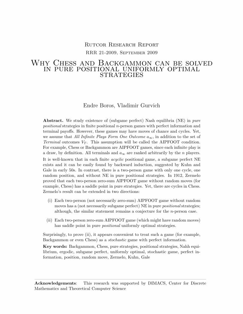
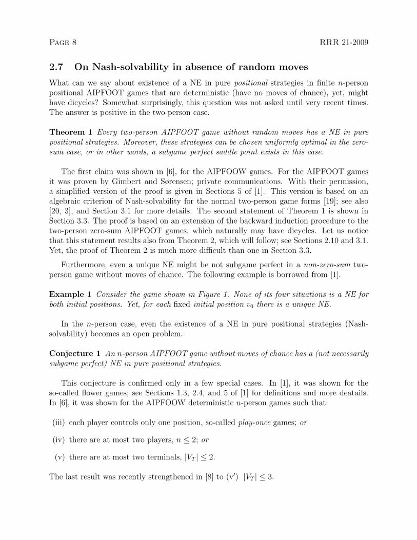
Example 1 Consider the game shown in Figure 1. None of its four situations is a NE forboth initial positions. Yet, for each fixed initial position v0 there is a unique NE.

In the n-person case, even the existence of a NE in pure positional strategies (Nash-solvability) becomes an open problem.

Conjecture 1 An n-person AIPFOOT game without moves of chance has a (not necessarilysubgame perfect) NE in pure positional strategies.

This conjecture is confirmed only in a few special cases. In [1], it was shown for theso-called flower games; see Sections 1.3, 2.4, and 5 of [1] for definitions and more deatails.In [6], it was shown for the AIPFOOW deterministic n-person games such that:

(iii) each player controls only one position, so-called play-once games; or

(iv) there are at most two players, n ≤ 2; or

(v) there are at most two terminals, |VT | ≤ 2.

The last result was recently strengthened in [8] to (v′) |VT | ≤ 3.

RRR 21-2009 Page 9

a1 a1 a1 a1

a2 a2 a2 a2

1 1 1 1

2 2 2 2

c ≺2 a2 a2 ≺1 a1 a2 ≺2 a1 a1 ≺1 c

Figure 1: A two-person game with one dicycle, two terminals, and no subgameperfect NE; the preferences are as follows: u1 : a2 ≺ a1 ≺ c and u2 : c ≺ a2 ≺ a1.In other words, player 1 prefers the cycle c the most, while player 2 dislikes it the most,and both players prefer a1 to a2. Thick lines represent the chosen strategies; the red oneindicates the choice which the player could switch and get a profit. Between the situationswe indicated the preference which make such a switch possible. In the first and third (thesecond and fourth) situations player 2 (respectively, 1) can improve. Since there are onlyfour situations, none of them is a NE for both initial positions simultaneously. Yet, for eachfixed initial position v0 there is a NE. If v0 is the position controlled by player 1 then thethird situation is a NE, while if v0 is controlled by player 2 then the second one is a NE.

Page 10 RRR 21-2009

2.8 Additive payoffs

In fact, claims (iii) and (iv) were proven in [6] in a more general setting. Given a digraphG = (V,E), let us define a local reward as a mapping r : I × E → R. Standardly, the valuer(i, e) is interpreted as the profit obtained by player i ∈ I whenever the play passes e ∈ E.

Let us recall that, in absence of random moves, each situation x ∈ X defines a uniqueplay p = p(x) that begins in the initial position v0 and either terminates at a(x) ∈ VT orresults in a simple dicycle c = c(x). The additive effective payoff u : I×X → R is defined inthe former case as the sum of all local rewards of the obtained play, u(i, x) =

∑e∈p(x) r(i, e),

and the latter case it is u(i, x) ≡ −∞ for all i ∈ I. In other words, all infinite plays areequivalent and ranked as the worst by all players, that is, we obtain a natural extension ofAIPFOOW games. Let us note however that in the first case payoffs depend not only on theterminal position a(x) but on the entire play p(x).

The following two assumptions were considered in [6]:

(vi) all local rewards are non-positive, r(i, e) ≤ 0 for all i ∈ I and e ∈ E and

(vii) all dicycles are non-positive,∑

e∈c r(i, e) ≤ 0 for all dicycles c ∈ C = C(G).

Obviously, (vi) implies (vii). Moreover, it was shown in 1958 by Gallai [13] that in fact thesetwo assumptions are equivalent, since (vi) can be enforced by a potential transformationwhenever (vii) holds; see [13] and also [6] for definitions and more details.

Remark 10 In [6], all players i ∈ I minimize cost function −u(i, x) instead of maximizingpayoff u(i, x). Hence, conditions (vi) and (vii) turn into non-negativity conditions in [6].

In [6], statements (iii) and (iv) are proven for the additive payoffs under assumptions (vi)and (vii); also several examples are given showing that these assumptions are essential.

It was also observed in [6] that the terminal AIPFOOW payoffs is a special case of theadditive AIPFOOW payoffs. To see this, let us just set r(i, e) ≡ 0 unless e is a terminal moveand notice also that no terminal move can belong to a dicycle. Hence, conditions (vi) and(vii) hold automatically in the special case of terminal AIPFOOW games. Thus, statements(iii) and (iv) follow from the corresponding claims proven in [6].

Remark 11 This reduction is similar to one that was sketched in the end of Introduction;it will be instrumental in the proof of Theorem 2.

In [6], Conjecture 1 is suggested for the additive AIPFOOW payoffs.

Conjecture 2 An AIPFOOW game with additive payoffs and without moves of chance hasa (not necessarily subgame perfect) NE in pure positional strategies whenever conditions (vi)and (vii) hold.

It was demonstrated in [6] that restrictions (vi), (vii), and AIPFOOW are essential.

Remark 12 Additive payoffs are considered only in this section; furthermore, other modifi-cations, such as cyclic and mean payoffs, will be considered in Sections 2.11 and 4.2 – 4.3,respectively; while the rest of the paper deals only with terminal AIPFOOT payoffs.

RRR 21-2009 Page 11

a3 a2

a1

3 2

1

×

p1

p2p3

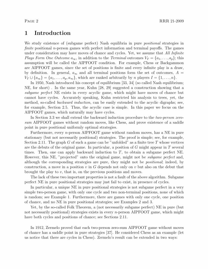
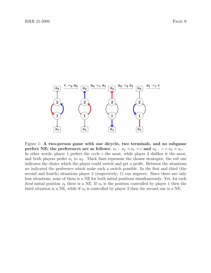
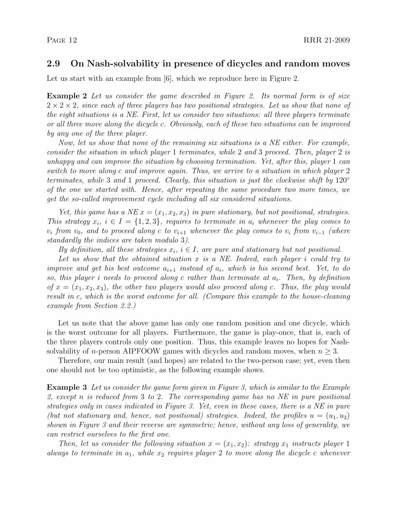
Figure 2: A three-person AIPFOOW game with one dicycle, one random position,and without NE in pure positional strategies. Each player i ∈ I = {1, 2, 3} has onlytwo options : either to move along the dicycle c or to terminate in ai. The last option is thesecond in the preference list of i; it is better (worse) if the next (previous) player terminates,while the dicycle itself is the worst option for all. In other words, the preference profile isu1 : a2 � a1 � a3 � c, u2 : a3 � a2 � a1 � c, u3 : a1 � a3 � a2 � c.Finally, there is a position of chance (in the middle) in which there are three moves tov1, v2, v3 with strictly positive probabilities p1, p2, p3, respectively.This game has no NE in pure positional strategies; see Example 2.However, there is a NE in pure stationary, but not positional, strategies.

Page 12 RRR 21-2009

2.9 On Nash-solvability in presence of dicycles and random moves

Let us start with an example from [6], which we reproduce here in Figure 2.

Example 2 Let us consider the game described in Figure 2. Its normal form is of size2× 2× 2, since each of three players has two positional strategies. Let us show that none ofthe eight situations is a NE. First, let us consider two situations: all three players terminateor all three move along the dicycle c. Obviously, each of these two situations can be improvedby any one of the three player.

Now, let us show that none of the remaining six situations is a NE either. For example,consider the situation in which player 1 terminates, while 2 and 3 proceed. Then, player 2 isunhappy and can improve the situation by choosing termination. Yet, after this, player 1 canswitch to move along c and improve again. Thus, we arrive to a situation in which player 2terminates, while 3 and 1 proceed. Clearly, this situation is just the clockwise shift by 120◦

of the one we started with. Hence, after repeating the same procedure two more times, weget the so-called improvement cycle including all six considered situations.

Yet, this game has a NE x = (x1, x2, x3) in pure stationary, but not positional, strategies.This strategy xi, i ∈ I = {1, 2, 3}, requires to terminate in ai whenever the play comes tovi from v0, and to proceed along c to vi+1 whenever the play comes to vi from vi−1 (wherestandardly the indices are taken modulo 3).

By definition, all these strategies xi, i ∈ I, are pure and stationary but not positional.Let us show that the obtained situation x is a NE. Indeed, each player i could try to

improve and get his best outcome ai+1 instead of ai, which is his second best. Yet, to doso, this player i needs to proceed along c rather than terminate at ai. Then, by definitionof x = (x1, x2, x3), the other two players would also proceed along c. Thus, the play wouldresult in c, which is the worst outcome for all. (Compare this example to the house-cleaningexample from Section 2.2.)

Let us note that the above game has only one random position and one dicycle, whichis the worst outcome for all players. Furthermore, the game is play-once, that is, each ofthe three players controls only one position. Thus, this example leaves no hopes for Nash-solvability of n-person AIPFOOW games with dicycles and random moves, when n ≥ 3.

Therefore, our main result (and hopes) are related to the two-person case; yet, even thenone should not be too optimistic, as the following example shows.

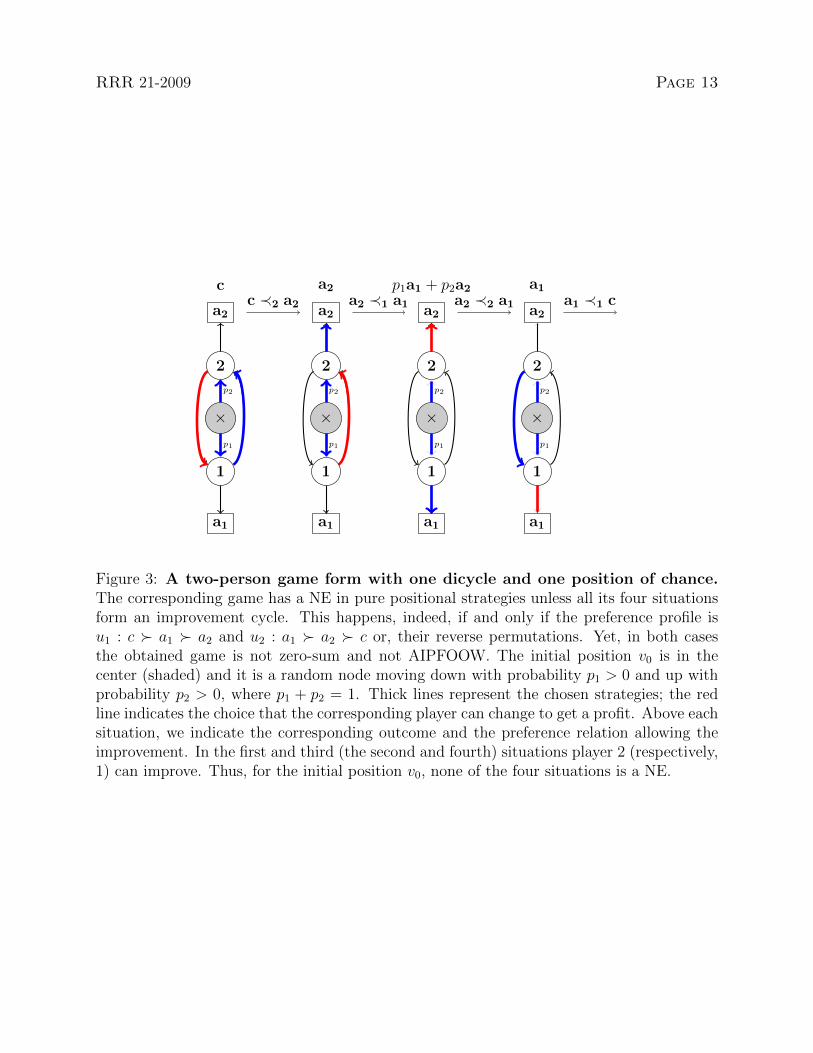
Example 3 Let us consider the game form given in Figure 3, which is similar to the Example2, except n is reduced from 3 to 2. The corresponding game has no NE in pure positionalstrategies only in cases indicated in Figure 3. Yet, even in these cases, there is a NE in pure(but not stationary and, hence, not positional) strategies. Indeed, the profiles u = (u1, u2)shown in Figure 3 and their reverse are symmetric; hence, without any loss of generality, wecan restrict ourselves to the first one.

Then, let us consider the following situation x = (x1, x2): strategy x1 instructs player 1always to terminate in a1, while x2 requires player 2 to move along the dicycle c whenever

RRR 21-2009 Page 13

a1 a1 a1 a1

a2 a2 a2 a2

1 1 1 1

2 2 2 2

× × × ×p1 p1 p1 p1

p2 p2 p2 p2

c ≺2 a2 a2 ≺1 a1 a2 ≺2 a1 a1 ≺1 cc a2 p1a1 + p2a2 a1

Figure 3: A two-person game form with one dicycle and one position of chance.The corresponding game has a NE in pure positional strategies unless all its four situationsform an improvement cycle. This happens, indeed, if and only if the preference profile isu1 : c � a1 � a2 and u2 : a1 � a2 � c or, their reverse permutations. Yet, in both casesthe obtained game is not zero-sum and not AIPFOOW. The initial position v0 is in thecenter (shaded) and it is a random node moving down with probability p1 > 0 and up withprobability p2 > 0, where p1 + p2 = 1. Thick lines represent the chosen strategies; the redline indicates the choice that the corresponding player can change to get a profit. Above eachsituation, we indicate the corresponding outcome and the preference relation allowing theimprovement. In the first and third (the second and fourth) situations player 2 (respectively,1) can improve. Thus, for the initial position v0, none of the four situations is a NE.

Page 14 RRR 21-2009

b2 2

b1

1

×

1

a1

2 a2

p1

q1

p2q2

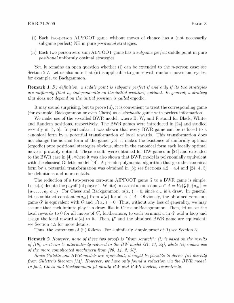
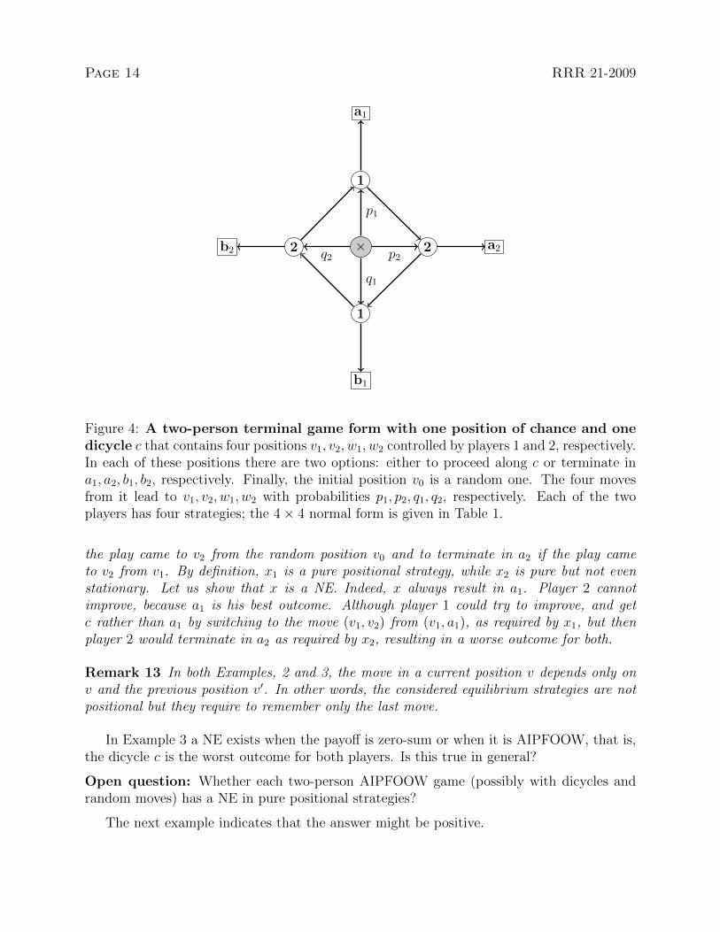
Figure 4: A two-person terminal game form with one position of chance and onedicycle c that contains four positions v1, v2, w1, w2 controlled by players 1 and 2, respectively.In each of these positions there are two options: either to proceed along c or terminate ina1, a2, b1, b2, respectively. Finally, the initial position v0 is a random one. The four movesfrom it lead to v1, v2, w1, w2 with probabilities p1, p2, q1, q2, respectively. Each of the twoplayers has four strategies; the 4× 4 normal form is given in Table 1.

the play came to v2 from the random position v0 and to terminate in a2 if the play cameto v2 from v1. By definition, x1 is a pure positional strategy, while x2 is pure but not evenstationary. Let us show that x is a NE. Indeed, x always result in a1. Player 2 cannotimprove, because a1 is his best outcome. Although player 1 could try to improve, and getc rather than a1 by switching to the move (v1, v2) from (v1, a1), as required by x1, but thenplayer 2 would terminate in a2 as required by x2, resulting in a worse outcome for both.

Remark 13 In both Examples, 2 and 3, the move in a current position v depends only onv and the previous position v′. In other words, the considered equilibrium strategies are notpositional but they require to remember only the last move.

In Example 3 a NE exists when the payoff is zero-sum or when it is AIPFOOW, that is,the dicycle c is the worst outcome for both players. Is this true in general?

Open question: Whether each two-person AIPFOOW game (possibly with dicycles andrandom moves) has a NE in pure positional strategies?

The next example indicates that the answer might be positive.

RRR 21-2009 Page 15

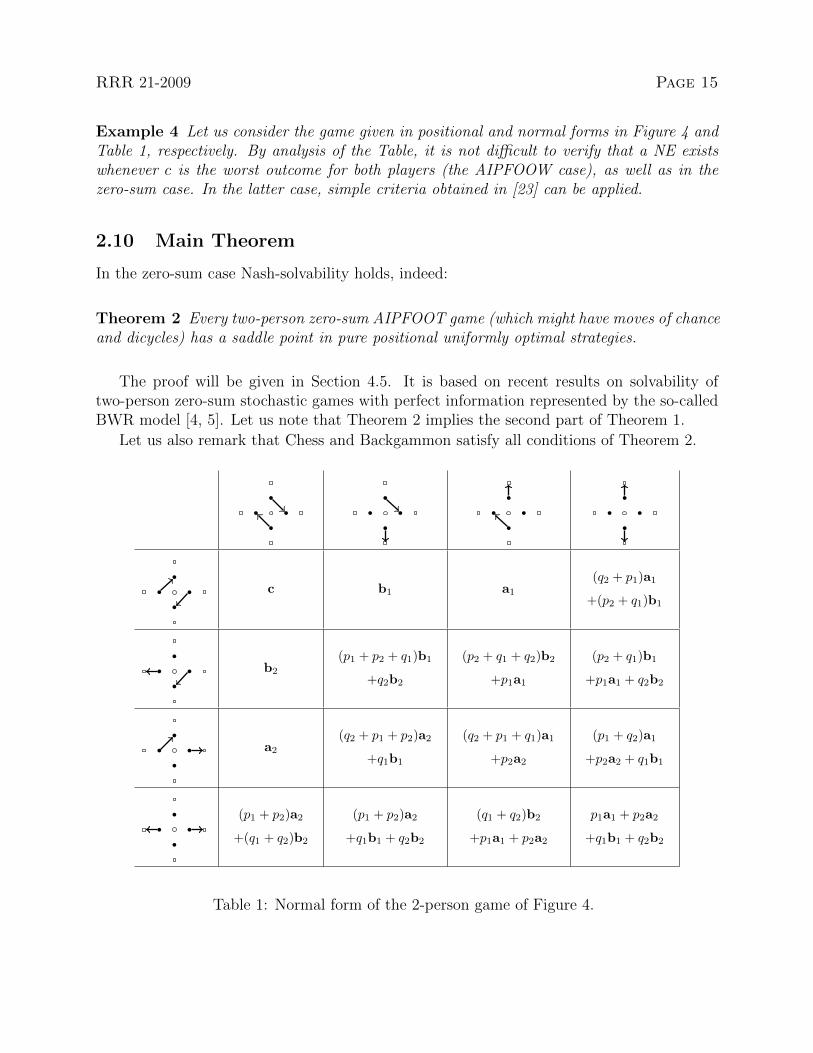
Example 4 Let us consider the game given in positional and normal forms in Figure 4 andTable 1, respectively. By analysis of the Table, it is not difficult to verify that a NE existswhenever c is the worst outcome for both players (the AIPFOOW case), as well as in thezero-sum case. In the latter case, simple criteria obtained in [23] can be applied.

2.10 Main Theorem

In the zero-sum case Nash-solvability holds, indeed:

Theorem 2 Every two-person zero-sum AIPFOOT game (which might have moves of chanceand dicycles) has a saddle point in pure positional uniformly optimal strategies.

The proof will be given in Section 4.5. It is based on recent results on solvability oftwo-person zero-sum stochastic games with perfect information represented by the so-calledBWR model [4, 5]. Let us note that Theorem 2 implies the second part of Theorem 1.

Let us also remark that Chess and Backgammon satisfy all conditions of Theorem 2.

c b1 a1(q2 + p1)a1

+(p2 + q1)b1

b2

(p1 + p2 + q1)b1

+q2b2

(p2 + q1 + q2)b2

+p1a1

(p2 + q1)b1

+p1a1 + q2b2

a2(q2 + p1 + p2)a2

+q1b1

(q2 + p1 + q1)a1

+p2a2

(p1 + q2)a1

+p2a2 + q1b1

(p1 + p2)a2

+(q1 + q2)b2

(p1 + p2)a2

+q1b1 + q2b2

(q1 + q2)b2

+p1a1 + p2a2

p1a1 + p2a2

+q1b1 + q2b2

Table 1: Normal form of the 2-person game of Figure 4.

Page 16 RRR 21-2009

2.11 Nash-solvability of n-person AIPFOOT games in pure butnot necessarily positional strategies; Folk Theorem

It is easy to get a (not necessarily subgame perfect) NE in pure and stationary (but notnecessarily positional) strategies in any AIPFOOT n-person game G = (G,P, v0, u) withoutrandom moves, for example, in Chess. The digraph G of such a game can be ”unfolded”and, thus, represented as a tree: Let us assume, without any loss of generality, that eachposition v of G can be reached by a simple directed path (dipath) d from v0; recall that d iscalled a debut. Let us add to d one more move (v, v′); the obtained dipath d′ will be calleda lasso if v′ belongs to d. Let us assign a position v(d) to every debut d (including all finiteplays) and a terminal position v(d′) to each lasso d′. Furthermore, let us draw a directededge from v to v′′ whenever d(v′′) is an extension (a lasso or not) of d(v). It is easily seenthat the obtained digraph G′ is a directed tree in which d(v0) is a root. Let us also note thatseveral positions of G′ may correspond to debuts of G ending at the same position.

A game G ′ = (G′, P ′, v′0, u′) is defined in an obvious way. The terminal vertices of G′

correspond to the lassos or finite plays, terminating at a ∈ VT . Let us assign payoffs byassociating u(i, a∞) for to a lasso and u(i, a) to a finite play, for all i ∈ I.

A NE in the obtained game G ′ can be determined by the classical backward induction.Obviously, the corresponding strategies in the original game G are pure (and even stationary)but they may not be positional. Indeed, by construction, a move in a position v = v(d) ischosen as a function of the debut d, not only of v.

Moreover, a subgame perfect NE in pure (but not necessarily positional or even station-ary) strategies exists in each AIPFOOT n-person game, which might have both dicyclesand random moves; see Examples 2 and 3. This result is usually referred to as the ”FolkTheorem”; so we shall not provide any other references. Let us derive it from Theorem 2.

For each player i ∈ I denote by u0i the maximal payoff that player i can guaranteein pure positional strategies and let xi be such a strategy. The corresponding situationx = (xi | i ∈ I) defines a Markov chain. Let ui denote the expected payoffs of the playeri ∈ I in this Markov chain. By definition, ui ≥ u0i for all i ∈ I. Furthermore, by thesame definition and Theorem 2, each other player j ∈ I \ {i} has a positional and ergodic”punishing” strategy xij such that i gets at most ui in the situation (xi) ∪ (xij | j ∈ I \ {i}).This follows, because ”punishing of player i” can be viewed as a two-person zero-sum game ofi against the complementary coalition I\{i}, where all coalitionists have the same preference,which is opposite to the preference of player i.

Then, let us modify the strategies xi ”slightly” to get strategies yi defined for all i ∈ Ias follows: yi = xi until each player i ∈ I applies xi; yet, if a player i ∈ I deviates from xithen all other players j ∈ I \ {i} immediately switch to their joint punishing strategies xij.Let us underline that the player who brakes the rule first is to get punished.

By construction, the situation y = (yi | i ∈ I) is a subgame perfect NE; moreover, allstrategies yi, i ∈ I, are pure and ergodic but not necessarily positional or even stationary.

Remark 14 By Theorem 2, all strategies xi and xjj were chosen positional. However, theresulting strategies yi are not even stationary, anyway. Hence, to prove Folk Theorem, it

RRR 21-2009 Page 17

would suffice to solve the considered two-person zero-sum ”punishing games” in pure but notnecessarily positional strategies. Of course, the existence of such strategies can be shownmuch simpler, without Theorem 2.

2.12 On Nash-solvability of bidirected cyclic two-person games

For completeness, let us survey one more result on Nash-solvability obtained in [7].

Let payoff u : I × (C ∪ VT )→ R be an arbitrary function, where C = C(G) denotes theset of dicycles of G. In this model, every dicycle c ∈ C, as well as each terminal a ∈ VT , is aseparate outcome, in contrast to the AIPFOOT case.

A digraph G is called bidirected if (v, v′) is its edge whenever (v′, v) is.

Necessary and sufficient conditions of Nash-solvability were announced in [15, 16, 17]for the bidirected bipartite cyclic two-person game forms. Recently, it was shown that thebipartitedness is in fact irrelevant. Necessary and sufficient conditions for Nash-solvabilityof bidirected cyclic two-person game forms were shown in [7].

3 Proof of Theorem 1

3.1 Equivalence of Nash- zero-sum- and ±1-solvabilities

Let us recall some of the basic definitions. Given a set of players I = {1, . . . , n} and outcomesA = {a1, . . . , ap}, an n-person game form g is a mapping g : X → A, where X =

∏i∈I Xi

and Xi is a finite set of strategies of player i ∈ I. Furthermore, a utility or payoff functionis a mapping u : I × A → R. Standardly u(i, a) is interpreted is a profit of player i ∈ I incase of outcome a ∈ A. A payoff u is called zero-sum if

∑i∈I u(i, a) = 0 for all a ∈ A.

The pair (g, u) is called a game in normal form.

Given a game (g, u) a strategy profile x ∈ X is a NE if u(i, g(x)) ≥ u(i, g(x′)) for everyi ∈ I and every x′ that differs from x only in coordinate i. A game form g is called Nash-solvable if for every utility function u the obtained game (g, u) has a NE.

Furthermore, a two-person game form g is called:

• zero-sum-solvable if for each zero-sum utility function the obtained zero-sum game(g, u) has a NE (which is called a saddle point for the zero-sum games);

• ±1-solvable if zero-sum solvability holds for each u that takes only values +1 and −1.

Necessary and sufficient conditions for zero-sum solvability were obtained by Edmondsand Fulkerson [9] in 1970; see also [18]. Somewhat surprisingly, these conditions remainnecessary and sufficient for Nash-solvability as well [19], see also [20] and [3]. Moreover, allthree types of solvability are equivalent for the two-person game forms but, unfortunately,not for the three-person ones [19, 20, 3].

Page 18 RRR 21-2009

3.2 Proof of the first statement of Theorem 1

We want to prove that every two-person AIPFOOT game without random moves has a NEin pure positional strategies.

Let G = (G,P, v0, u) be such a game, in which u : I × A → {−1,+1} is a zero-sum ±1utility function. As we just mentioned, it would suffice to prove solvability in this case [19].

Let Ai ⊆ A denote the outcomes winning for player i ∈ I = {1, 2}. Let us also recallthat Vi ⊆ V denotes the subset of positions controlled by player i ∈ I = {1, 2}.

Without any loss of generality, we can assume that c ∈ A1, that is, u(1, c) = 1, whileu(2, c) = −1, or in other words, player 1 likes dicycles. Let W 2 ⊆ V denote the set ofpositions in which player 2 can enforce (not necessarily in one move) a terminal from A2,and let W 1 = V \W 2. By definition, player 2 wins whenever v0 ∈ W 2. Let x2 denote sucha winning strategy; note that x2 can be defined arbitrarily in V2 ∩W 1.

We have to prove that player 1 wins whenever v0 ∈ W 1. Indeed, for an arbitrary vertexv, if v ∈ W 1 ∩V2 then player 2 cannot leave W 1, that is, v′ ∈ W 1 for every move (v, v′) ∈ E.Furthermore, if v ∈ W 1∩V1 then player 1 can stay in W 1, that is, (s)he has a move (v, v′) ∈ Esuch that v′ ∈ W 1. Let player 1 choose such a move for every position v ∈ W 1 ∩ V1 andarbitrary moves in all remaining positions, from W 2 ∩ V1. This rule defines a strategy x1 ofplayer 1. Let us show that x1 wins whenever v0 ∈ W 1. Indeed, in this case the play cannotenter W 2. Hence, it either will terminate in A1 or result in a di cycle; in both cases player1 wins. Thus, player 1 wins when v0 ∈ W 1, while player 2 wins when v0 ∈ W 2. �

Remark 15 We proved a little more than we planed to, namely, in case of ±1 zero-sumpayoffs the obtained strategies x1 and x2 are positional and uniformly optimal, or in otherwords, that situation x = (x1, x2) is a subgame perfect saddle point. Moreover, in the nextsection we will extend this result to all (not only ±1 zero-sum games. However, it cannotbe extended further, since a non-zero-sum two-person AIPFOOT game might have, in purepositional strategies, a unique NE, which is not subgame perfect; see Example 1.

3.3 Backward induction in presence of dicycles andproof of the second statement of Theorem 1

As we already mentioned, the second part of Theorem 1 is a special case of Theorem 2. Yet,it can be proved simpler, by a generalization of the arguments from the previous section.

We want to show that every two-person zero-sum AIPFOOT game without random moveshas a saddle point in pure positional uniformly optimal strategies. Let G = (G,P, v0, u) besuch a game. The results of the previous two sections imply that the value µ = µ(v) andoptimal positional pure strategies x1(v) and x2(v) exist for every initial position v. Yet, westill have to prove that there are positional uniformly optimal strategies, as well.

In the previous section, this was already shown for the zero-sum ±1 payoffs. Now, weextend this proof to the case of arbitrary zero-sum payoffs. In fact, we extend the backwardinduction procedure to work in the presence of dicycles. However, this extension will workonly for the two-person zero-sum AIPFOOT games without moves of chance.

RRR 21-2009 Page 19

Let us first determine the value µ(v) for each possible initial position v ∈ V .Since the game is zero-sum, we simplify notation by introducing u(1, a) = u(a) and

u(2, a) = −u(a) for every outcome a ∈ A = VT ∪ {a∞}, and view player 1, White, as amaximizer, and player 2, Black, as a minimizer.

We shall apply two reduction phases, recursively:Phase 1. Let us start with the standard backward induction and proceed until possible:Given a position v ∈ V1 (respectively, v ∈ V2) such that every move (v, a) from v leads to aterminal position a ∈ VT , let us chose in v a move (v, a) = x1(v) maximizing (respectively,(v, a) = x2(v) minimizing) the value u(a). Obviously, such a move should be required by anyuniformly optimal strategy. Then let us delete all moves from v, thus, making it a terminalposition, and define payoff u(v) = u(a) in it. This (backward induction) procedure can berepeated until either:

(viii) we got rid of all arcs, or

(ix) a non-terminal move exists in every non-terminal position v ∈ V1 ∪ V2 = V \ VT .

Case (viii) means that G is an acyclic digraph and pure positional uniformly optimalstrategies x1 and x2 in game G are found by the standard backward induction. Otherwise,we obtain a reduced game G ′ satisfying condition (ix).

Furthermore, each pair (x′1, x′2) of pure positional uniformly optimal strategies in game G ′

can obviously be extended to such strategies in the original game G, by selecting the abovechosen moves. Hence, condition (ix) can be assumed without any loss of generality.

Phase 2. Let us set µ1 = max{µ(v)} and µ2 = min{µ(v)} where max and min are taken overall positions v ∈ V1∪V2 = V \VT , and define W1 = {v | µ(v) = µ1} and W2 = {v | µ(v) = µ2}.Let us recall that u(a∞) is the payoff in case of an infinite play. By (ix), we obtain:

W1 ∩ V1 6= ∅ if and only if µ1 ≥ u(a∞) andW2 ∩ V2 6= ∅ if and only if µ2 ≤ u(a∞).

If Wi ∩ Vi 6= ∅ for some i ∈ I = {1, 2} then we must have a position v ∈ Wi ∩ Vi in whichthere is a terminal move (v, a), a ∈ VT , such that u(a) = µ(v) = µi. In other words, move(v, a) gives player i the best possible result; in particular, it is not worse than an infiniteplay. Obviously, such a move might be chosen by a uniformly optimal strategy.

Then, let us set xi(v) = (v, a) , delete all moves from v, thus, making it a terminalposition, and define the terminal payoff u(v) = u(a) in it.

Let us note that, after this, we may be able to perform some reductions by Phase 1 oncemore. If we arrive again to condition (ix), we just repeat the above Phase 2 reduction.

Let us also remark that, after each step, the interval [µ1, µ2] may only shrink, in whichcase it should be updated. It is easy to see that, after a finite number of steps, either

(x) we get rid of all arcs, or

(xi) each terminal move is strictly worse for the controlling player than an infinite play.

Page 20 RRR 21-2009

In both cases, we can obtain pure positional uniformly optimal strategies.In case (x), it is obvious that the strategies x1 and x2 have all required properties.Otherwise, we obtain a reduced game G ′′ satisfying conditions (ix) and (xi).Obviously, in this case the interval [µ1, µ2] is reduced to a single point µ1 = µ2 = u(a∞).It is also clear that pure positional uniformly optimal strategies x′′1 and x′′2 exist. Indeed,

it is necessary, by (xi), and possible, by (ix), for each player to choose a non-terminal movein every position. Thus, x′′(x′′1, x

′′2) is a subgame perfect saddle point in G ′′ that yields an

infinite play p(x′′) which realizes the ergodic value µ = u(a∞).The obtained strategies x′′1 and x′′2 in G ′′ can obviously be extended to pure positional

uniformly optimal strategies in the original game G. �

Remark 16 In fact, our arguments combine and extend the original Zermelo, Kuhn, andGale approaches [37, 28, 12]. We just treat dicycles properly, to obtain strategies that areboth positional and uniformly optimal.

4 Proof of Theorem 2

4.1 Mean payoff n-person games

Let us recall the model of Section 2.1 and introduce the following modifications. First, letus get rid of the terminals; to do so, we just add a loop (v, v) to each terminal v ∈ VT .

Then, as in Section 2.9, let us introduce a local reward r : I×E → R, which value r(i, e)is standardly interpreted as a profit obtained by the player i ∈ I whenever the play passesthe arc e. A reward function r is called

• zero-sum if∑

i∈I r(i, e) = 0 for all e ∈ E.

• terminal if r(e) = 0 unless e is a loop.

Assume that all players are restricted to their pure positional strategies. Then, eachsituation x = (xi | i ∈ I) ∈ X =

∏i∈I Xi defines a Markov chain on G. This chain has

a limit distribution, which defines the expected reward u(x) = (u(i, x) | i ∈ I). Functionu(i, x) is the effective payoff in situation x, and called the mean payoff.

As we know, in the deterministic case, when VR = ∅, a situation x defines a play p(x)that results in a lasso, since there are no terminals. In this case, the effective payoff is theaverage (mean) payoff over the dicycle c = c(x) of this lasso:

u(i, x) = |c(x)|−1∑e∈c(x)

r(i, e) for all players i ∈ I and situations x ∈ X,

where |c| is the length of a dicycle c, that is, the number of its vertices or edges.

In the literature on mean-payoff games, usually the two-person zero-sum case is consid-ered, since not much is known in other cases. We also will restrict ourselves to this case

RRR 21-2009 Page 21

too, except for Section 4.3. Thus, we arrive to the BWR model, as it was defined earlier.Recall that B and W stand for ”Black” (player 2) who is minimizing, and ”White” (player1) who is maximizing, respectively, while R means ”random”. Since r(1, e) + r(2, e) = 0 forall e ∈ E, it will be convenient to set r(e) = r(1, e) just remembering that r(2, e) = −r(e).

4.2 Mean payoff games, BW model

In the deterministic case, when VR = ∅, we obtain the so called mean payoff BW games.In 1976, Moulin introduced these games in his PhD Thesis [31]; see also [32]. In fact, he

studied strategic extensions of matrix games, rather than stochastic games, and asked thequestion: which extensions have always a saddle point? The classical mixed extension givesan example. Yet, this extension is infinite. Can it be finite?

Given a k × ` matrix, Moulin introduced a large, but finite, k` × `k extension, in whicha strategy of a player is a function of (called as reply to) the opponent’s strategy. Givensuch two reply functions and an initial strategy v0 in the original k × ` matrix game, bothplayers take turns choosing their replies and this process results in an infinite play. Since thematrix is finite, this play consists of an initial part, if any, and an infinitely repeated cycle.The effective payoff is defined as the mean payoff over this cycle. Then, from the BrouwerFixed Point Theorem, Moulin derived the existence of a saddle point in pure strategies forthe obtained k` × `k matrix game.

In fact, Moulin’s games are the BW games on complete bipartite digraphs. In addition,the equality r(e) = r(e′) must hold for every pair of ”opposite” moves e = (v1, v2) ande′ = (v2, v1), where positions v1 and v2 are the strategies of the players 1 and 2, respectively.

Moulin also proved that such a game is ergodic, that is, its value does not depend onthe original strategy v0. For this reason, he called the obtained games ergodic extensionsof matrix games. Yet, this name appears not very lucky, because ergodicity holds for thecomplete bipartite digraphs but for some other digraphs, the value might depend on theinitial position. In fact, ergodic game forms are fully characterized in [25]. However, it isimportant to note that in any BW game there are ergodic (or uniformly optimal) strategies,which form a saddle point for every initial position v0.

Moreover, such pure positional uniformly optimal strategies exist not only in Moulin’smodel but in general, for any BWR game. This fact will imply Theorem 2.

In 1979, Ehrenfeucht and Mycielski introduced BW games for all (not only complete)bipartite graphs and gave a combinatorial proof of the existence of a saddle point [11]. Their,very short abstract appeared already in 1973 [10].

In 1988, the model was extended to arbitrary (not only bipartite) digraphs in [24].Given a real potential π : V → R, the local reward function r : E → R can be transformed

by the formula rπ(v, v′) = r(v, v′) + π(v) − π(v′). Such transformation changes the normalform of the game in a trivial way: the constant π(v0) is added to all efficient payoffs.

In [24] an algorithm of potential reduction was suggested that brings the game to acanonical form in which the solution is obvious, since every locally optimal move is just

Page 22 RRR 21-2009

optimal. Thus, we obtain uniformly optimal strategies of both players. In contrast, thevalue of a BW game might depend on the initial position.

BW games are of serious interest for complexity theory, because the decision problem”whether the value of a BW game is positive” belongs to NP ∩ coNP [27], yet, no polynomialalgorithm is known yet; see, for example, the survey [36].

4.3 A NE-free non-zero-sum two person mean payoff game

Let us continue by observing that Nash-solvability fails for the non-zero-sum mean payoffBW games. Already the ergodic extension of a 3×3 bimatrix game might not have NE. Thefollowing example was given in [21]; see also [24]:

0 0 1 1 0 0ε 0 0 0 1 00 ε 0 1− ε 0 1

Here ε is a small positive number, say, 0.1. Standardly, the first and second 3×3 matricesdefine the payoffs for players 1 and 2, respectively. The corresponding normal form is of size33 × 33 = 27 × 27. Its entries are mean payoffs defined, in accordance with the above twomatrices, on the dicycles of the complete bipartite 3 × 3 digraph. Let us choose the bestdicycle for player 1 (respectively, 2) in each column (row) of the normal form. The obtainedtwo sets of dicycles are disjoint [21]. Hence, there is no NE. In contrast, it was shown in [22]that the ergodic extensions of 2× k bimatrix games are always Nash-solvable.

In other words, a mean payoff BW game has a NE in pure positional ergodic strategieswhenever its digraph is complete bipartite and of size 2 × k, yet, this statement cannot beextended to the case of the 3 × 3 digraphs. This negative result shows that our proof ofTheorem 2 cannot be extended to the non-zero-sum case, although, by Theorem 1, in thiscase, Nash-solvability holds. However, in Example 1, a unique NE exists for each of the twoinitial positions but the corresponding two NE are distinct.

4.4 Stochastic games with perfect information and the BWR model

The mean payoff BWR games were introduced in [24], yet, main results were obtained in[24] only for the BW games; they were extended to the BWR case just recently, in [4, 5].

In particular, it was shown that for the BWR games a canonical form exists and it canbe obtained by a potential transformation method. The main two properties of canonicalforms for the mean payoff BW and BWR games are similar:

• The normal form of the game is modified in a predictable way, namely, the value π(v0)is added to the effective payoff in each situation x ∈ X;

• In each position, the locally optimal moves (that maximizes for White player 1, orminimizes for Black player 2) the local payoff r are provably optimal.

RRR 21-2009 Page 23

The latter property implies that the obtained optimal strategy is uniformly optimal (ergodic),that is, it does not depend on the initial position. In contrast, the value of the game mightdepend on it.

Yet, the proof for the BWR case is substantially more complicated than for the BW one.Along with mean payoff games δ-discounted payoff must also be considered. For this case, thepotential transformation should be ”slightly” modified to rπ(v, v′) = r(v, v′) +π(v)− δπ(v′)[24]. The technical derivation is based on non-trivial results of the Tauberian theory and,in particular, on the Hardy-Littlewood Theorem [26], which provide sufficient conditionsfor the Abel and Cesaro averages (which correspond to the discounted and mean payoffs,respectively) to converge to the same limit. The verification of these conditions in case ofMarkov chains is based on deep results by Blackwell [2]. It is also shown in [4] that the meanpayoff BWR model is polynomially equivalent with the classical Gillette model [14].

Remark 17 Of course, the careful reader noticed that we applied similar techniques, asGillette in his paper [14]. In 1953 Shapley introduced stochastic games with non-zero stopingprobability [35]. Then, in 1957 Gillete extended the analysis to a difficult case of zero-stop probability. In particular, he introduced the mean payoff stochastic games with perfectinformation and, for this case, proved solvability in pure ergodic positional strategies.

The Hardy-Littlewood Theorem is instrumental in Gillette’s arguments, too. By the way,his paper contained a repairable flaw: conditions of Hardy-Littlewood’s theorem were notaccurately verified. (Let us recall that the Blackwell paper [2] did not appear yet.) Thisflaw was corrected in 1969 by Liggett and Lippman [30]. As we already mentioned in theIntroduction, it may be possible to derive Theorem 2 from Gillete’s result rather than theBWR model. Yet, the latter is still of independent interest and also it is ”closer to thesubject”. Indeed, the reduction of parlour games, like Chess and Backgammon, to meanpayoff BWR games is immediate; see the Introduction or the next Section. However, it isnot that simple, although it might be possible, to represent these games in the Gilette model.

4.5 Reduction of AIPFOOT games to terminal BWR games andproof of Theorem 2

In fact, we have not much to add to the proof sketched in Introduction, yet, all necessarydefinitions are available by now. To prove Theorem 2, it would be sufficient to consider onlytwo-person zero-sum AIPFOOT games. Yet, the following reduction works in general.

Let G = (G,P, v0, u) be an n-person AIPFOOT game and u(i, c) be the payoff of playeri ∈ I in case of an infinite play. Let us reduce the payoff function u by vector u(c) = (u(i, c) |i ∈ I), that is, for all i ∈ I let us set u′(i, v) = u(i, v)−u(i, c) for each v ∈ VT and u′(i, c) = 0.Clearly, the obtained AIPFOOT game G ′ = (G,P, v0, u

′) is trivially related to G and everyinfinite play ”becomes a draw” in G ′, like in Chess or Backgammon.

Let us add a loop ev = (v, v) to each terminal v ∈ VT , then set r(i, ev) = u′(i, v) andr(i, e) = 0 for all arcs of G and players i ∈ I. The following five statements are obvious:

• the obtained terminal BWR game G ′′ is equivalent to G ′ and, hence, to G;

Page 24 RRR 21-2009

• the mapping G ′′ ↔ G is a bijection;

• the game G has no moves of chance if and only if G ′′ is a BW game;

• the obtained terminal BWR payoff in G ′′ is strictly positive, that is r(i, ev) > 0 for allplayers i ∈ I and loops ev = (v, v), v ∈ V , if and only if G is an AIPFOOW game;

• games G and G ′′ can be zero-sum games only simultaneously.

Thus, if G is a two-person zero-sum game then so is G ′′. It was shown in [4, 5] thatG ′′ has a saddle point in pure positional uniformly optimal strategies. Obviously, the samestrategies form a saddle point in game G. �

Remark 18 Note that games without positions of chance, like Chess, are reduced to BWgames, which are much easier to solve and analyze than BWR games.

Moreover, solvability of Chess in pure positional uniformly optimal strategies results alsofrom Theorem 1, which, in its own turn, follows from the equivalence of Nash-, zero-sum,and ±1-solvabilities [9, 18, 19]).

5 State of the art

Finite positional n-person games with perfect information are considered. In absence ofdicycles everything is simple. Each acyclic game has a subgame perfect NE in pure posi-tional strategies. One of these NE (so-called sophisticated or dominance equilibrium) can beobtained by the backward induction procedure suggested by Kuhn [28, 29] and Gale [12].

Next, let us assume that dicycles might exist but All Infinite Plays Form One Outcome,a∞ or c, in addition to the Terminal outcomes VT = {a1, . . . , ap}. This assumption is calledthe AIPFOOT condition. For example, Chess and Backgammon are AIPFOOT games,because an infinite play is a draw, by definition.

First, let us assume that there are no positions of chance, like in Chess, for example.For this case, Zermelo [37] proved his famous theorem that can be reformulated as follows:

a two-person zero-sum AIPFOOT game without random moves has a saddle point x =(x1, x2) in pure strategies. Theorem 1 extends this result in two directions:

Strategies x1 and x2 can be chosen positional and uniformly optimal.

A (not necessarily subgame perfect) NE in pure positional strategies exists in anytwo-person AIPFOOT game without random moves, even in the non-zero-sum case.

To prove the first statement, we modify the classical backward induction procedure forthe two-person zero-sum AIPFOOT games, which might have dicycles; see Section 3.3.

Furthermore, we conjecture that the last statement can be extended to the n-person case,Conjecture 1. It was proved for the play-once AIPFOOW games in [6] and by Gimbert and

RRR 21-2009 Page 25

Sørensen for the two-person AIPFOOT games. Their proof can be simplified by recallingthat Nash-solvability and ±1-solvability are equivalent for the two-person game forms [19].However, this observation cannot be extended to the n-person case with n > 2 [19, 20, 3].

Already for n = 2, a unique NE might be not subgame perfect [1]; see Example 1.Recently in [8], Conjecture 1 was proven for the case of at most three terminals.In [6], Conjecture 1 was suggested in a more general setting of additive payoffs, yet, only

for the AIPFOOW games and non-negative local cost functions, Conjecture 2. It was shownthat both above restrictions are essential and that Conjecture 2 is stronger than Conjecture 1.Finally, the first one was proved in two special cases: play-once and two-person AIPFOOWgames.

Now, let us assume that both dicycles and moves of chance may exist. Even in this, mostgeneral, case the existence of a subgame perfect NE in pure (but not necessarily positionalor even stationary) strategies can be derived from the so-called Folk Theorem; Section 2.11.

In absence of random moves, these strategies can be chosen ergodic pure and stationary,but still, not necessarily positional. The proof is based on the observation that each finitedigraph can be ”unfolded” as a tree; see Section 2.11 again.

In this paper, we concentrate on (subgame perfect) NE in pure positional strategies. Thefollowing negative observations should be taken into account: Example 2 gives a three-personplay-once AIPFOOW game with only one dicycle, one position of chance, and no NE in purepositional strategies and, thus, leaves no hope for Nash-solvability in the case of n ≥ 3.Moreover, Example 3 provides a game that has all above properties but it is not AIPFOOWand n is reduced from 3 to 2; the game is not zero-sum, either. This leaves two open ends:

The first one, whether a NE in pure positional strategies always exists in the two-personAIPFOOW games, is still open.

The second one, whether each two-person zero-some AIPFOOT game has a saddle pointin pure positional uniformly optimal strategies is answered by Theorem 2 in the affirmative.This result is proved by the reduction of the n-person AIPFOOT games to stochastic gameswith perfect information. In particular, two-person zero-sum AIPFOOT games are reducedto the BWR games. For the latter, the solvability in pure positional uniformly optimalstrategies was recently shown in [4, 5].

Finally, let us remark that two-person zero-sum AIPFOOT games without random moves,like Chess, are reduced to the BW games, for which solvability in pure positional uniformlyoptimal strategies is much easier to show [32, 11, 24] than for the BWR games.

Acknowledgements:We are thankful to Khaled Elbassioni and Kazuhisa Makino, our colleagues in BWR studies;the second author also thanks Daniel Anderson, Stephane Gaubert, Hugo Gimbert, ThomasDueholm Hansen, Nick Kukushkin, Peter Bro Miltersen, Troels Bjerre Sørensen, and SylvainSorin for helpful discussions.

Page 26 RRR 21-2009

References

[1] D. Anderson, V. Gurvich, and T. Hansen, On acyclicity of games with cycles, RUTCORResearch Report RRR-18-2008 and DIMACS Technical Report 2009-09, Rutgers Uni-versity; Algorithmic Aspects in Information and Management (AAIM); Lecture Notesin Computer Science 5564 (2009) 15-28.

[2] D. Blackwell, Discrete dynamic programming, Annals of Mathematical Statistics 33(1962) 719726.

[3] E. Boros, K. Elbassioni, Gurvich, and K. Makino, On effectity functions of game forms,RUTCOR Research Report, RRR-03-2009; Games and Economic Behaviour, to appear;http://dx.doi.org/10.1016/j.geb.2009.09.002

[4] E. Boros, K. Elbassioni, Gurvich, and K. Makino, Every stochastic game with perfectinformation admits a canonical form, RUTCOR Research Report, RRR-09-2009.

[5] E. Boros, K. Elbassioni, Gurvich, and K. Makino, A pumping algorithm for ergodicstochastic mean payoff games, RUTCOR Research Report, RRR-19-2009.

[6] E. Boros and V. Gurvich, On Nash-solvability in pure strategies of finite games withperfect information which may have cycles. Math. Social Sciences 46 (2003), 207-241.

[7] E. Boros, V. Gurvich, K. Makino, and Wei Shao, Nash-solvable bidirected cyclic two-person game forms, DIMACS Technical Report, DTR-2008-13 and RUTCOR ResearchReport, RRR-30-2007, revised in RRR-20-2009, Rutgers University.

[8] E. Boros and R. Rand, Terminal games with three terminals have proper Nash equilibria,RUTCOR Research Report, RRR-22-2009, Rutgers University.

[9] J. Edmonds and D.R. Fulkerson, Bottleneck extrema, J. of Combinatorial Theory, 8(1970), 299-306.

[10] A. Ehrenfeucht and J. Mycielski, Positional games over a graph, Notices of the AmericanMathematical Society 20 (1973) A-334, Abstract.

[11] A. Ehrenfeucht and J. Mycielski, Positional strategies for mean payoff games, Interna-tional Journal of Game Theory 8 (1979), 109-113.

[12] D. Gale, A theory of N -person games with perfect information, Proc. Natl. Acad. Sci.39 (1953) 496–501.

[13] T. Gallai, Maximum-minimum Satze uber Graphen, Acta Mathematica Academiae Sci-entiarum Hungaricae 9 (1958) 395–434.

RRR 21-2009 Page 27

[14] D. Gillette, Stochastic games with zero stop probabilities; in Contribution to the Theoryof Games III, in Annals of Mathematics Studies 39 (1957) 179–187; M. Dresher, A.W.Tucker, and P. Wolfe eds, Princeton University Press.

[15] A.I. Gol’berg and V.A. Gurvich, Tight cyclic game forms, Russian Mathematical Sur-veys, 46:2 (1991) 241-243.

[16] A.I. Gol’berg and V.A. Gurvich, Some properties of tight cyclic game forms, RussianAcad. Sci. Dokl. Math., 43:3 (1991) 898-903.

[17] A.I. Gol’berg and V.A. Gurvich, A tightness criterion for reciprocal bipartite cyclicgame forms, Russian Acad. Sci. Dokl. Math., 45 (2) (1992) 348-354.

[18] V. Gurvich, To theory of multi-step games, USSR Comput. Math. and Math. Phys. 13:6(1973) 143-161.

[19] V. Gurvich, Solution of positional games in pure strategies, USSR Comput. Math. andMath. Phys. 15:2 (1975) 74-87.

[20] V. Gurvich, Equilibrium in pure strategies, Doklady Akad. Nauk SSSR 303:4 (1988)538-542 (in Russian); English translation in Soviet Math. Dokl. 38:3 (1989) 597-602.

[21] V. Gurvich, A stochastic game with complete information and without equilibriumsituations in pure stationary strategies, Russian Math. Surveys 43:2 (1988) 171–172.

[22] V. Gurvich, A theorem on the existence of equilibrium situations in pure stationarystrategies for ergodic extensions of (2× k) bimatrix games, Russian Math. Surveys 45:4(1990) 170–172.

[23] V. Gurvich, Saddle point in pure strategies, Russian Acad. of Sci. Dokl. Math. 42:2(1990) 497–501.

[24] V. Gurvich, A. Karzanov, and L. Khachiyan, Cyclic games and an algorithm to findminimax cycle means in directed graphs, USSR Computational Mathematics and Math-ematical Physics 28:5 (1988) 85-91.

[25] V.A. Gurvich and V.N. Lebedev, A criterion and verification of ergodicity of cyclic gameforms, Russian Mathematical Surveys, 44:1 (1989) 243-244.

[26] G. H. Hardy and J. E. Littlewood, Notes on the theory of series (XVI): two Tauberiantheorems, J. of London Mathematical Society 6 (1931) 281–286.

[27] A.V. Karzanov and V.N. Lebedev, Cyclical games with prohibition, Mathematical Pro-gramming 60 (1993), 277-293.

[28] H. Kuhn, Extensive games, Proc. Natl. Acad. Sci. 36 (1950) 286–295.

Page 28 RRR 21-2009

[29] H. Kuhn, Extensive games and the problem of information, in Contributions to thetheory of games, Volume 2, Princeton (1953) 193–216.

[30] T.M. Liggett and S.A. Lippman, Stochastic Games with Perfect Information and TimeAverage Payoff, SIAM Review 11 (1969) 604607.

[31] H. Moulin, Prolongement des jeux a deux joueurs de somme nulle, Bull. Soc. Math.France, Memoire 45, 1976.

[32] H. Moulin, Extension of two person zero-sum games, Journal of Mathematical Analysisand Application 55 (2) (1976) 490-508.

[33] J. Nash, Equilibrium points in n-person games, Proceedings of the National Academyof Sciences 36 (1) (1950) 48-49.

[34] J. Nash, Non-Cooperative Games, Annals of Mathematics 54:2 (1951) 286–295.

[35] L. S. Shapley, Stochastic games, in Proc. Nat. Acad. Science, USA 39 (1953) 1095–1100.

[36] S. Vorobyov, Cyclic games and linear programming, Discrete Applied Mathematics 156(11) (2008) 2195–2231.

[37] E. Zermelo, Uber eine Anwendung der Mengenlehre auf die Theorie des Schachspiels;in: Proc. 5th Int. Cong. Math. Cambridge 1912, vol. II; Cambridge University Press,Cambridge (1913) 501-504.