Why Functional Programming Matters

Roger Costello

May 31, 2013

In the first paper (Part 1) I summarized the first half of John Hughes' outstanding paper titled,

Why Functional Programming Matters. It described how higher-order functions can be used to

modularize programs. Here's the URL to my first paper:

http://xfront.com/Haskell/Why-Functional-Programming-Matters.pdf

This paper (Part 2) summarizes the second half of Hughes' paper, which describes the use of lazy

evaluation and composition for modularizing programs.

I converted all the programs in Hughes' paper to Haskell.

Lazy Evaluation plus Composition is the Most Powerful Tool for Successful Programming Composition enables whole programs to be glued together. Recall that a complete functional

program is just a function from its input to its output. If f and g are such programs, then (g . f) is a

program which, when applied to its input, computes

g (f input)

The program f computes its output which is used as the input to program g. This might be

implemented conventionally by storing the output from f into a temporary file. The problem with

this is the temporary file might occupy so much memory that it is impractical to glue the

programs together in this way.

Functional languages provide a solution to this problem. The two programs f and g are run

together in strict synchronization. f is only started once g tries to read. Then f is suspended and g

is run until it tries to read another input. As an added bonus, if g terminates without reading all of

f’s output then f is aborted.

f can even be a non-terminating program, producing an infinite amount of output, since it will be

terminated forcibly as soon as g is finished. This allows termination conditions to be separated

from loop bodies – a powerful modularization.

Since this method of evaluation runs f as little as possible, it is called "lazy evaluation." It makes

it practical to modularize a program as a generator which constructs a large number of possible

answers, and a selector which chooses the appropriate one. While some other systems allow

programs to be run together in this manner, only functional languages use lazy evaluation

uniformly for every function call, allowing any part of a program to be modularized in this way.

Lazy evaluation is perhaps the most powerful tool for modularization in the functional

programmer's repertoire.

What is the Opposite of Lazy Evaluation? In a programming language that does lazy evaluation, computations are delayed until they are

needed. The opposite of this is to perform all computations; this is called "eager evaluation."

To get an intuition of the difference between lazy and eager evaluation, consider this if-then-else

statement:

if 1==1 || error("blah") then "error not evaluated" else "unreachable"

In a lazy evaluation, the if-then-else produces this output: error not evaluated

In an eager evaluation, the if-then-else produces this error: blah

Here's why: The condition 1==1 || error("blah") has two parts. With lazy evaluation only the first

part is evaluated; since 1==1 evaluates to true, it is not necessary to evaluate the other part of the

condition. With eager evaluation both parts are evaluated, which results in the error function

being invoked and thereby generating an error.

Problem #1: Pruning Infinite (or Very Long) Lists of Values

Modularity is the key to successful programming. [John Hughes]

Lazy evaluation is perhaps the most powerful tool for modularization in the functional

programmer's repertoire. Consider …

Most functional programming languages have a function called "repeat" which generates an

infinite list; its argument is used as the value of the list. For example, this generates an infinite

list of 3:

repeat 3 returns [3, 3, 3, …]

Also provided by most functional programming languages is a function called "take" which has

two arguments, an integer N and a list. The function "take" returns the first N values of the list.

"take" can be composed with "repeat" to obtain a pruned list of values. The following returns the

first 5 values of an infinite list:

take 5 . repeat

Function composition is denoted by the dot ( . )

Applying that composed function to 3 results in a list of five 3's:

(take 5 . repeat) 3 returns [3, 3, 3, 3, 3]

It is lazy evaluation that allows us to modularize the pruning problem in this way. The "repeat"

function is evaluated lazily – only as many values as requested are generated. So lazy evaluation

is very efficient. Without lazy evaluation we would have to fold these two functions together into

one function which only constructs the first five values.

Here is another example. We can define the set of even numbers by enumerating all positive

numbers [1..] and multiplying each by 2:

evens = [ x * 2 | x <- [1..] ]

That is, of course, an infinite list. However, lazy evaluation will compute only as many as

needed. Let's take the first 5 evens:

take 5 evens returns [2, 4, 6, 8, 10]

An association list is a list of pairs, where the first element represents the index of the second

element, e.g.:

[ (0,'h'), (1,'e'), (2,'l'), (3,'l'), (4,'o') ]

Given a list xs, it can be converted into an association list by zipping (0, 1, 2, …) with xs, e.g.:

zip [0..] "hello"

[0..] is an infinite list, but due to lazy evaluation only as much of the list that is needed is actually

generated.

One more example. The example comes from the field of Artificial Intelligence. A decision tree

is generated. It could be a decision tree for medical diagnosis or a decision tree for chess moves

or a decision tree for something else. The decision tree is potentially infinite. Without lazy

evaluation, processing may never terminate. Rather than exploring a potentially infinite space we

prune the tree to a depth of, say, 5 levels:

prune 5 . decisiontree

decisiontree is a function that generates the tree. prune 5 chops off any levels of the tree beyond 5

levels deep. We can make improvements by tinkering with each part. Without lazy evaluation we

would have to fold these two functions into one function which only constructed the first five

levels of the tree. That is a significant reduction in modularity.

See Problem #4 below for an implementation of the game of Tic-Tac-Toe.

Lesson Learned: Want to have successful software? Then you need to learn how to take

advantage of the enhanced modularity that lazy evaluation provides. And, of course, you need to

use a programming language that supports lazy evaluation.

Problem #2: Square Root Finder We will illustrate the power of lazy evaluation by creating a program that finds square roots. As

we proceed please note the insistence on creating generic modules that can be used in solving

many problems.

The square root of n can be found by starting with an initial approximation a0 and then

computing better and better approximations, a1,a2, a3, …. We can compute an+1 by taking an,

adding n divided by an, and then dividing by 2:

an+1 = (an + n/an)/2

For example, let's compute the square root of 2. Let's take 1 as the initial approximation.

a0 = 1 a1 = (1 + 2/1)/2 = 1.5 a2 = (1.5 + 2/1.5)/2 = 1.4166666666666665 a3 = (1.4166666666666665 + 2/1.4166666666666665)/2 = 1.4142156862745097 etc.

Each approximation gets better and better. The difference between an and an-1 gets smaller and

smaller.

Since this approach to finding the square root involves computing a list of approximations it is

natural to represent this as a list. First, let's define a function that computes the next

approximation:

next n x = (x + n/x) / 2

Let a0 = 1. Then the list of approximations is produced by calling next with a0, then calling next

with next a0, then calling next with next (next a0), and so forth:

[a0, next a0, next (next a0), …]

So next is repeatedly called and each result is appended onto the list. It goes on forever – it is a

potentially infinite list.

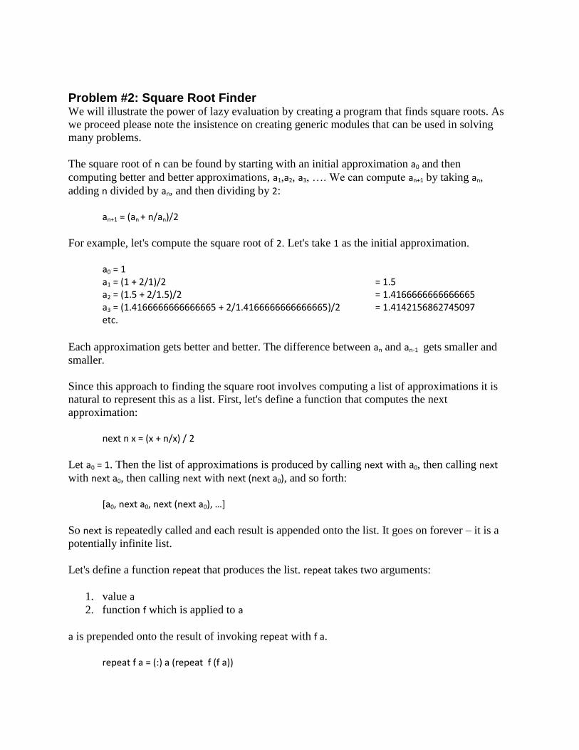
Let's define a function repeat that produces the list. repeat takes two arguments:

1. value a

2. function f which is applied to a

a is prepended onto the result of invoking repeat with f a.

repeat f a = (:) a (repeat f (f a))

repeat is a wonderful, re-usable module. It can be used with any function f.

For the square root problem we want to repeatedly call the function next:

repeat (next 2) 1

That generates a list of approximations of the square root of 2, with an initial approximation of 1:

[1.0,1.5,1.4166666666666665,1.4142156862745097,1.4142135623746899,1.414213562373095,1.414213562373095,1.414213562373095,...

The list is infinite. repeat is an example of a function with an "infinite" output. But that doesn't

matter because no more approximations will actually be computed than the rest of the program

requires. The "infinity" is only potential. Any number of approximations can be computed if

required, repeat itself places no limit.

The repeat function is a powerful tool for modularization. A user of the repeat function can focus

on generating the list. The user does not need to be concerned with implementing a search

algorithm and defining a termination condition, that problem is left to another function. That is a

beautiful modularization.

The remainder of the square root finder is a function within that takes a delta and a list of

approximations and looks down the list for the first two successive approximations that differ by

no more than delta.

within delta (x:y:zs) | abs(x-y) <= delta = y

| otherwise = within delta (y:zs)

"Take the (absolute) difference between the first two elements of the list, x and y. If the

difference between x and y is less than delta then return the second element. Otherwise, search

the list starting at y."

Putting the parts together, we define sqrt as follows:

sqrt a0 delta n = within delta (repeat (next n) a0)

That is a fantastic function.

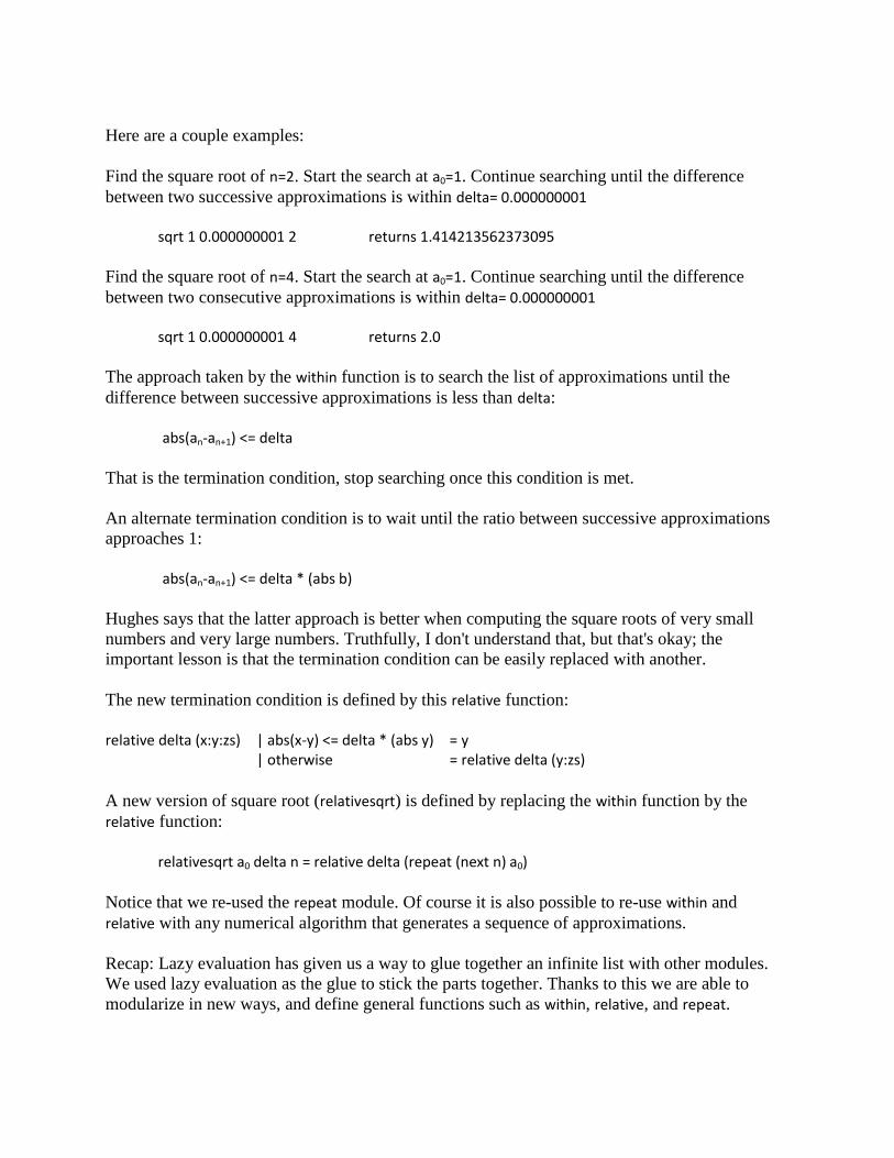
Here are a couple examples:

Find the square root of n=2. Start the search at a0=1. Continue searching until the difference

between two successive approximations is within delta= 0.000000001 sqrt 1 0.000000001 2 returns 1.414213562373095

Find the square root of n=4. Start the search at a0=1. Continue searching until the difference

between two consecutive approximations is within delta= 0.000000001 sqrt 1 0.000000001 4 returns 2.0

The approach taken by the within function is to search the list of approximations until the

difference between successive approximations is less than delta:

abs(an-an+1) <= delta

That is the termination condition, stop searching once this condition is met.

An alternate termination condition is to wait until the ratio between successive approximations

approaches 1:

abs(an-an+1) <= delta * (abs b)

Hughes says that the latter approach is better when computing the square roots of very small

numbers and very large numbers. Truthfully, I don't understand that, but that's okay; the

important lesson is that the termination condition can be easily replaced with another.

The new termination condition is defined by this relative function:

relative delta (x:y:zs) | abs(x-y) <= delta * (abs y) = y

| otherwise = relative delta (y:zs)

A new version of square root (relativesqrt) is defined by replacing the within function by the

relative function:

relativesqrt a0 delta n = relative delta (repeat (next n) a0)

Notice that we re-used the repeat module. Of course it is also possible to re-use within and

relative with any numerical algorithm that generates a sequence of approximations.

Recap: Lazy evaluation has given us a way to glue together an infinite list with other modules.

We used lazy evaluation as the glue to stick the parts together. Thanks to this we are able to

modularize in new ways, and define general functions such as within, relative, and repeat.

Problem #3: Finding the Slope of a Function Recall from your math classes that the slope of a line is "rise over run." That is, the change in y

divided by the change in x. Here is the graph of the function x2:

Suppose we wish to find the slope at the black dot. Take another dot on the graph, connect the

two dots and find the rise over run:

This gives a crude approximation of the slope at the point. We can get a better approximation by

taking a point that is nearer:

We can get better and better approximations by taking points closer and closer.

Let's take a point h units from x (along the x-axis). Then the slope is:

slope f x h = (f(x+h)-(f x))/h

The particular function, f, that we are examining is f = x2 (squared):

squared = (\x -> x * x)

Let's determine the slope of squared at the point x=0.5 by performing the calculation with h=4,

h=2, and h=1:

slope squared 0.5 4 -- returns 5.0 slope squared 0.5 2 -- returns 3.0 slope squared 0.5 1 -- returns 2.0

Recall the repeat function:

repeat f a = (:) a (repeat f (f a))

It generates a list of values [a, f a, f (f a), f (f (f a)), …]

Here's a function that halves a value:

halve = (\x -> x / 2)

Let's use it in the repeat function to generate the next value.

The following generates an infinite list of h values, starting at h=4:

repeat halve 4

That is, it generates:

[4.0, 2.0, 1.0, 0.5, 0.25, 0.125, ... ]

We will use that list for h values in our slope function. Let's call this list, the h-list.

Recall the slope function:

slope f x h = (f(x+h)-(f x))/h

The third argument to slope is h. Let's apply slope to each h value in the h-list. Recall that map f

list applies f to each element of list. So let's use map to apply the partial function (slope f x) to each

element of the h-list:

map (slope f x) (repeat halve h0)

Here's an example:

map (slope squared 0.5) (repeat halve 4) -- returns [5.0,3.0,2.0,1.5,1.25,… ]

That returns a list of slope approximations, so let's name it slope_approximations:

slope_approximations h0 f x = map (slope f x) (repeat halve h0)

Recall the within function:

within delta (x:y:zs) | abs(x-y) <= delta = y

| otherwise = within delta (y:zs)

within takes a delta and a list of approximations and searches the list for two successive

approximations that differ by no more than delta.

Let's use it to search the list of slope approximations:

within delta (slope_approximations h0 f x)

Here's an example:

within 0.000000001 (slope_approximations 4 squared 0.5) -- returns 1.0

Thus, the slope of the function x2 at x=0.5 is 1.

Hughes' paper then shows how to improve the list of approximations. Truthfully, it involves

some math that I don't feel like digging into. However, what does interest me is that this infinite

list of slope approximations can be improved. Obviously an infinite list cannot be created and

then improved. Rather, the list is created as needed and then improved as needed. That is neat.

Problem #4: Using Lazy Evaluation in Artificial Intelligence

The AI community often solves problems by building and traversing "decision trees." A tree is

built that consists of all possible choices, a "local goodness" value is assigned to each choice

using local information, and then the "true goodness" is determined for a choice from the local

goodnesses in the subtrees.

We will use that AI technique to code a tic-tac-toe game. Well, actually we won't code the entire

game. We will build a "game board tree" consisting of all possible moves, we will assign a

"static" value to each game board using local information, and then we will determine a "true"

value of a game board based on the static values of the subtrees. The objective is to demonstrate

that lazy evaluation enables a nice modularization of the code. Without lazy evaluation many of

the modules would necessarily have to be merged into one large module, which makes tweaking

parts of the code difficult.

Note: I allow the game board to be any square grid (2x2, 3x3, etc.). Many of my examples use

2x2 game boards but the implementation works for any sized board.

A game board is represented by a list of (x,y) positions plus player. For example, this game

board:

is represented by this list:

[ ( (0,0), X ), ( (1,0), O ), ( (1,1), X ) ]

A player's position on the board is of type Pos:

type Pos = (Int, Int)

The game is played between a computer and an opponent. The computer marks the board with O

and the opponent with X:

data Player = O | X computer = O opponent = X

The dimensions of the game board are specified by width/height values. For example, a 2x2

board is specified like so:

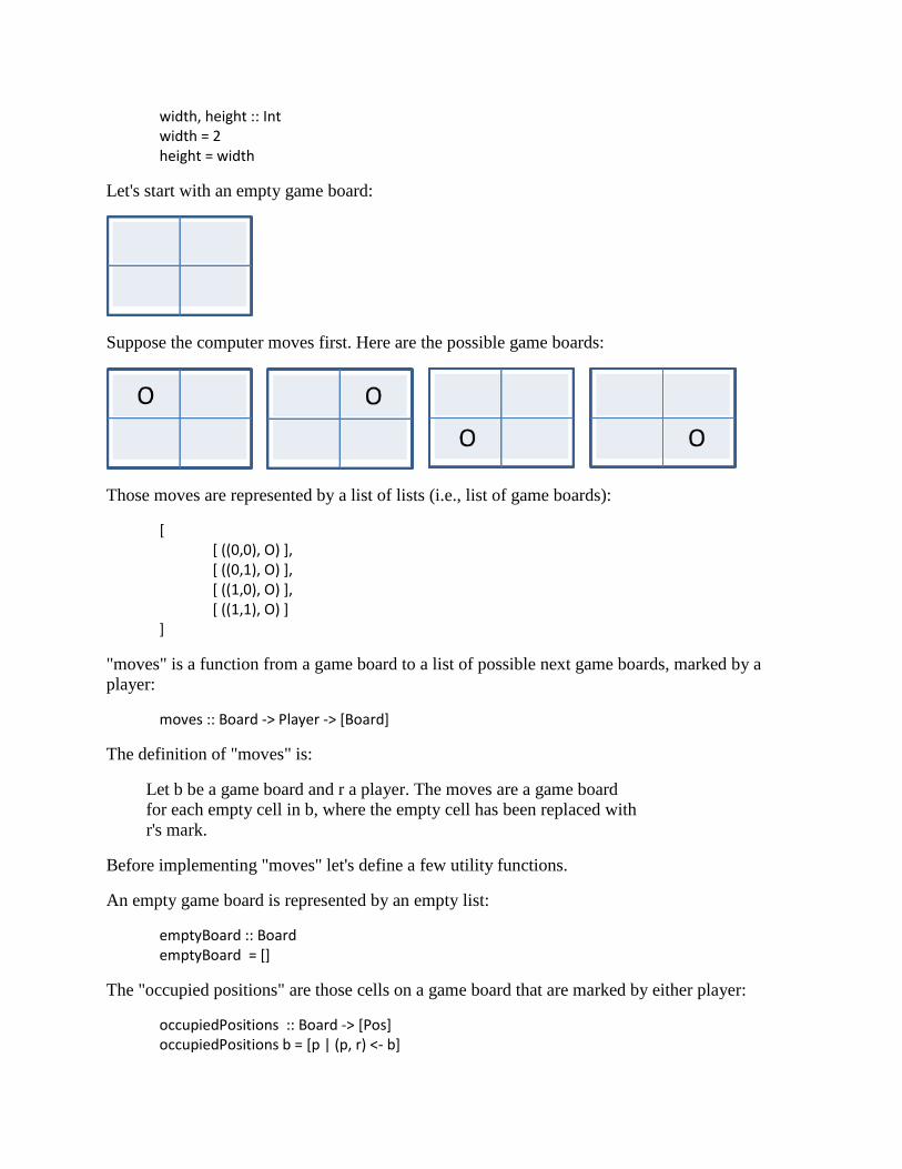
width, height :: Int width = 2 height = width

Let's start with an empty game board:

Suppose the computer moves first. Here are the possible game boards:

Those moves are represented by a list of lists (i.e., list of game boards):

[ [ ((0,0), O) ], [ ((0,1), O) ], [ ((1,0), O) ], [ ((1,1), O) ] ]

"moves" is a function from a game board to a list of possible next game boards, marked by a

player:

moves :: Board -> Player -> [Board]

The definition of "moves" is:

Let b be a game board and r a player. The moves are a game board

for each empty cell in b, where the empty cell has been replaced with

r's mark.

Before implementing "moves" let's define a few utility functions.

An empty game board is represented by an empty list:

emptyBoard :: Board emptyBoard = []

The "occupied positions" are those cells on a game board that are marked by either player:

occupiedPositions :: Board -> [Pos] occupiedPositions b = [p | (p, r) <- b]

A particular cell is marked if it is an element of "occupied positions":

isMarked :: Board -> Pos -> Bool isMarked b p = elem p (occupiedPositions b)

A particular cell is empty (unmarked) if it is not marked:

isEmpty :: Board -> Pos -> Bool isEmpty b p = not (isMarked b p)

The "available cells" is the list of empty cells:

available :: Board -> [Pos] available b = [(x,y) | x <- [0..(width-1)], y<- [0..(height-1)], isEmpty b (x,y)]

Okay, now we are ready to define the "moves" function. The result of invoking "moves" is a list

of boards, each board contains one new mark on one of the available cells:

moves :: Board -> Player -> [Board] moves b r = [(p,r):b | p <- available b]

Important: Arranging the set of possible game boards into a tree structure considerably

simplifies processing.

A gametree is a tree consisting of all possible moves. Here is a portion of a gametree:

Initially the game board is empty, as shown by the root node. The computer moved first and

there are four possible game boards, as shown by the second row of the tree. From each of these

boards the opponent has three possible moves. And so forth.

Here is a recursive data type that can represent any kind of tree:

data Treeof a = Node a [Treeof a]

Before creating the gametree, let's create a higher-order function that can create any tree

(conforming to the Treeof data type). The function is named "reptree" (repeating tree). The

"reptree" function is given a function "f " and a value "a". The root node is defined to have the

value "a". Applying f to "a" produces a list of values. That is, (f a) produces [a1, a2, …, an]. Each

of those values is the root node of a subtree, so reptree is applied to each of them. Here is the

definition of reptree:

reptree is a root node "a" and each child node (subtree) is a reptree. The

subtrees are produced by applying reptree to f(a).

reptree is implemented by using map to apply (reptree f) to each value generated by (f a):

reptree f a = Node a (map (reptree f) (f a))

We will invoke reptree with the moves function and a game board. Recall that the moves function

takes two arguments: a game board and a player. So we need to make a small modification to the

reptree function. Actually, we need to make two modifications. We need two reptree functions,

one for the situation where the computer moves first and one for the situation where the

opponent moves first:

reptree f a = Node a (map (reptree' f) (f a computer))

reptree' f a = Node a (map (reptree f) (f a opponent))

The first version, reptree, is used to generate moves when the computer makes the first move.

For each of the boards that it generates it invokes reptree' which does the same thing except the

opponent is the player. Do you see how reptree will generate game boards for every other level

of the game tree and reptree' will generate game boards for the other levels? For example, reptree

generates the game boards for Level 2 and then reptree' generates the game boards for Level 3

and then reptree generates the game boards for Level 4 and then reptree' generates the game

boards for Level 5 and so forth.

So a gametree is a reptree where f is the moves function and a is a Board. A gametree is created

by invoking reptree with the moves function and a game board:

gametree :: Board -> Treeof Board gametree b = reptree moves b

gametree invokes reptree, which as we've seen assumes that the computer makes the first move.

We want to allow the opponent to make the first move, so let's create a second version of

gametree which invokes reptree'.

gametree' :: Board -> Treeof Board gametree' b = reptree' moves b

To create a complete gametree, invoke the gametree function (or gametree') with an empty board:

gametree emptyboard

Here is a portion of the output:

Node [] [ Node [((0,0),O)] [ Node [((0,1),X),((0,0),O)] [ Node [((1,0),O),((0,1),X),((0,0),O)] [ Node [((1,1),X),((1,0),O),((0,1),X),((0,0),O)] [] ], Node [((1,1),O),((0,1),X),((0,0),O)] [ Node [((1,0),X),((1,1),O),((0,1),X),((0,0),O)] [] ] ], Node [((1,0),X),((0,0),O)] [ Node [((0,1),O),((1,0),X),((0,0),O)] [ Node [((1,1),X),((0,1),O),((1,0),X),((0,0),O)] [] ], Node [((1,1),O),((1,0),X),((0,0),O)] [ Node [((0,1),X),((1,1),O),((1,0),X),((0,0),O)] [] ] ],

Let's review what we've accomplished. We implemented a moves function that, when given a

game board and player it returns a list of game boards representing the next possible moves for

the player. Next, to facilitate processing, we implemented a gametree that consists of all possible

moves, where alternating Levels of the tree are one player's moves and the other Levels of the

tree are the other player's moves.

Our goal is to implement an evaluate function that a player can use to choose the best next move.

(Actually, our goal is to show that the implementation of the evaluate function has superior

modularity due to lazy evaluation.) To accomplish this we will implement the following

functions:

1. static: the purpose of this function is to give a rough estimate of the value of a game

board without looking at any of the other game boards. The simplest implementation is to

return +1 for game boards where the computer has won, -1 for game boards where the

opponent has won, and 0 otherwise.

2. evaluate: the purpose of this function is to determine the best next move. Whereas the

"static" function assigns each game board a score using local information, the "evaluate"

function assigns each board a score by looking down the gametree at the static values in

descendant nodes and generating an aggregate score from them. This function will be

implemented using an algorithm developed by the AI community called the alpha-beta

heuristic (also called the minmax algorithm).

Let's start by implementing the "static" function. It takes a game board and returns 1 if the

computer has won, -1 if the opponent has won, and 0 otherwise:

static :: Board -> Integer

For the moment, let's assume the existence of a "won" function that takes a game board, a player,

and returns True if the player has won and False otherwise:

won :: Board -> Player -> Bool

We will show its implementation later on.

Now the "static" function is readily implemented:

static :: Board -> Integer static b = if (won b computer) then 1 else if (won b opponent) then (-1) else 0

We will apply static to each board in the gametree. The part 1tutorial defined a generic "maptree"

function that applies a function f to every node in a tree. Here we use maptree to apply static to

each board in the gametree:

maptree static . gametree

Here is a picture of a portion of the gametree and the corresponding tree of static values:

Notice at the bottom of the tree that the computer has won.

Hence, the number one ( 1 ) was assigned to those nodes in the static tree.

Game Board With Two Winners?

The tree shown above is just a portion of the tree. Suppose we take this board:

and apply the "moves" function to it:

The lower game board has two winners:

That's a problem. I spoke with a colleague and he said, "That's an impossible state." Okay, then

how do I prevent that impossible state? Should the "moves" function be modified to stop (return

an empty list) when it is given a game board that already has a winner? That seems reasonable.

The disadvantage, I think, is that now the moves function has to perform two tasks: create a set of

next game boards and determine if a game board has a winner. Isn't it best to create functions

that perform only one task? What are your thoughts on this? Please email me and let me know

your thoughts on this issue.

I modified the "moves" function to stop (return an empty list) when it is given a game board that

already has a winner:

moves :: Board -> Player -> [Board] moves b r | won b computer = [] | won b opponent = [] | otherwise = [(p,r):b | p <- available b]

There are two consequences of this change: (1) A gametree may be asymmetric because there are

no child nodes of a winning board. (2) There may be leaf nodes that represent a fully marked

board in which no one won.

We can make an optimization in our implementation. Consider: For a 2 x 2 game board the

maximum potential depth of the gametree is 5. For a 3 x 3 game board the maximum potential

depth of the gametree is 10 and the gametree will be huge. So let's implement a "prune" function

that chops off any subtrees beyond a depth of "n":

prune :: Int -> Treeof a -> Treeof a prune 0 (Node a xs) = Node a [] prune n (Node a xs) = Node a (map (prune (n-1)) xs)

Here we generate a gametree that does not look ahead more than 5 Levels:

prune 5 . gametree

This static tree does not look ahead more than 5 Levels:

maptree static . prune 5 . gametree

Pruning is a necessary activitity in games where the number of possible Levels of the tree are

large, such as in the game of chess. However, for tic-tac-toe the maximum number of Levels is

10, which I think is acceptable. So we will not use the prune function.

We are almost done. The final thing to implement is the evaluate function. The purpose of the

function is, given a game board, evaluate it for suitability as the next move. Obviously each

player wants the next move to maximize his chance of winning. The algorithm we will use to

implement the evaluate function is called the alpha-beta heuristic (also known as the minmax

function).

The static function assigns +1 to a game board if the computer has won, -1 if the opponent has

won, and 0 otherwise. Clearly, a game board is a great next move for the computer if its static

value is +1. Suppose we are evaluating game board A and its static value is 0. Is it a better next

move than game board B which also has a static value of 0? Here's one strategy (for the

computer): Game board A is a better next move than game board B if there are more +1 static

values in A's subtree than in B's subtree. A higher count represents a greater likelihood of

success.

Suppose we count the +1 static values in A's subtree and count the +1 static values in B's subtree

and the counts are the same, which game board is better? They seem to be equally good. But

suppose we also count the -1 static values in A's subtree and it is greater than the count of -1

static values in B's subtree, now which game board is better? B's game board is better because

there are less chances for the opponent to win. So we want to select the game board that has the

maximum number of +1 values and the minimum number of -1 values in its subtree. That is, the

computer wants to maximize its chances of winning and minimize the chances of its opponent

winning. This strategy of maximizing one variable and minimizing another is called the minmax

algorithm.

In the gametree every alternating level of the tree corresponds to the same player. Suppose the

computer starts the game and gets the first move. The root of the tree is the empty boad. Let's

call the root of the tree Level 0. Level 1 of the tree contains the potential game boards after one

move by the computer. Level 2 of the tree contains the potential game boards after one move by

the computer followed by one move by the opponent. Level 3 of the tree contains the potential

game boards after a move by the computer, then a move by the opponent, and then another move

by the computer. And so forth.

Suppose it is the computer's turn to move and it evaluates game board b. Suppose b is at Level i

in the game tree. If the computer decides to move to b then the subtree of b (Level i+1) will be

evaluated by the opponent and the opponent will select a board that gives him the best chance of

winning by selecting a board with a minimum evaluation value. For whatever board the

opponent selects, the computer will then evaluate its subtree (Level i+2) and select a board that

gives it the best change of winning by selecting a board with the maximum evaluation value.

And so forth.

So the computer wants the maximum of the opponent's minimum evaluation value. The

opponent wants the minimum of the computer's maximum evaluation value.

Here is how to maximize an evaluation value for a node in the game tree with static value n: if

the node is a leaf node then return n; otherwise, return the maximum of the minimum of its

subtrees:

maximize (Node n []) = n maximize (Node n subtrees) = maximum (map minimize subtrees)

Here is how to minimize an evaluation value for a node in the game tree with static value n: if

the node is a leaf node then return n; otherwise, return the minimum of the maximum of its

subtrees:

minimize (Node n []) = n minimize (Node n subtrees) = minimum (map maximize subtrees)

The computer evaluates a game board, b, by generating its game tree, generating the

corresponding static tree, and then taking the maximum of the minimum of the subtrees of b:

evaluate = maximize . maptree static . gametree

The opponent evaluates a game board, b', by generating its game tree, generating the

corresponding static tree, and then taking the minimum of the maximum of the subtrees of b':

evaluate' = minimize . maptree static . gametree

Let's take an example. Suppose that the computer has just moved; the resulting board is b and its

gametree is this:

The opponent needs to decide its next move among b's three subtrees. Clearly the first two

subtrees are desirable since the opponent could win and the computer cannot. The third subtree is

the not desirable since the opponent cannot win and the result is a draw. Let's see if the minmax

evaluation algorithm comes to the same conclusion. First, assign a static value to each board in

the game tree:

Next, evaluate each subtree of b. Let's start with the leftmost subtree. Through recursion, the

evaluate function will arrive at the leaf node and use its static value as its evaluation value (I use

"S" to denote Static value and "E" to denote Evaluation value. Also notice that I labeled each

Level of the tree to indicate whether it represents moves by the Opponent or the Computer):

Move up one Level. It is the Computer's move. In the left subtree the Opponent has just returned

with its evaluation which is a list of one value, [0]. The Computer seeks the maximum value,

which is 0. The right subtree is a leaf node, immediately return its Static value:

Move up another Level. It is the Opponent's move. The Computer has just returned with its

evaluation which is a list of two values, [0, -1]. The Opponent seeks the minimum value, which

is -1.

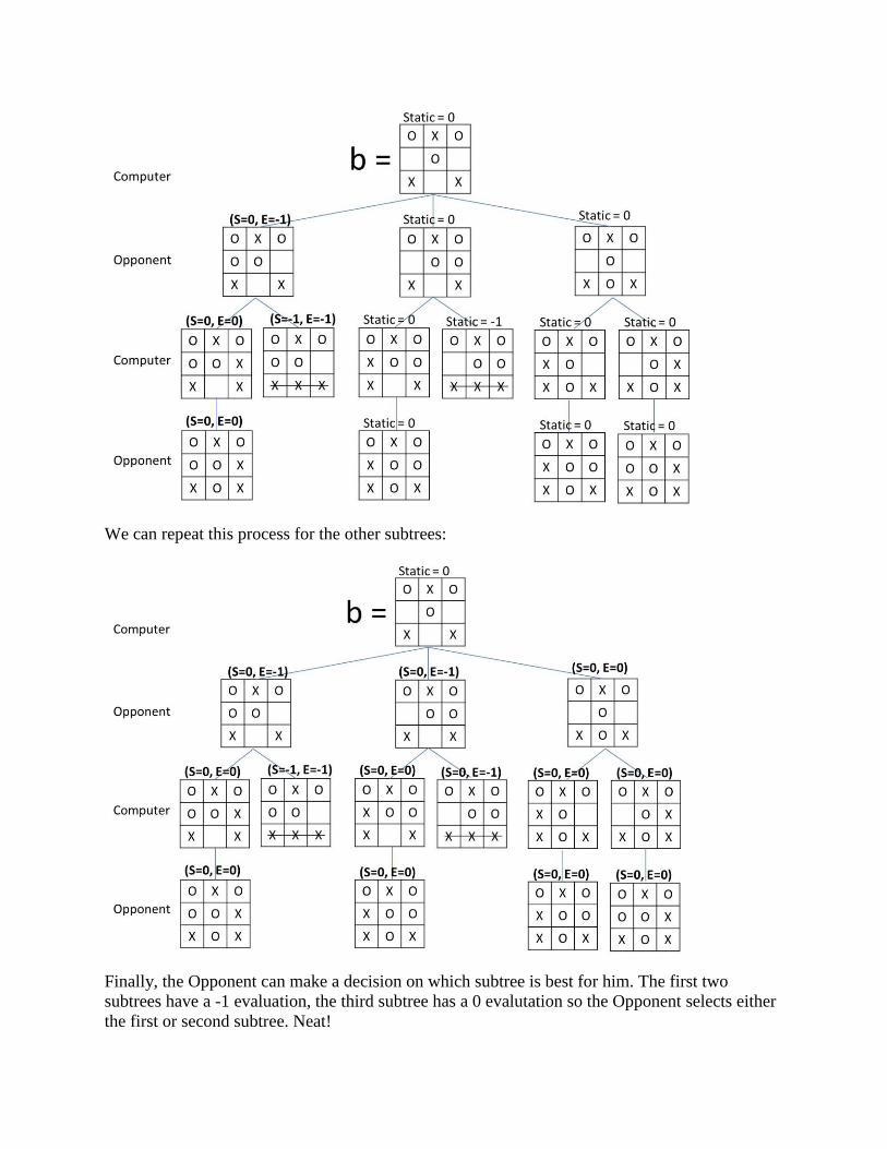
We can repeat this process for the other subtrees:

Finally, the Opponent can make a decision on which subtree is best for him. The first two

subtrees have a -1 evaluation, the third subtree has a 0 evalutation so the Opponent selects either

the first or second subtree. Neat!

We are done with our implementation of tic-tac-toe (the complete code is shown below). Now

for a brief analysis.

Pruning the Gametree

Although the game of tic-tac-toe is guaranteed to terminate, there are some games which may

never terminate; that is, the players could move forever. (I believe that some chess games could

continue forever.) In such never-ending games the game tree would be infinite and the evaluate

function would never return, so it would be important to use the prune function described above.

For example, this restricts the evaluate function to not look ahead more than 5 moves:

evaluate = maximize . maptree static . prune 5 . gametree

The Importance of Lazy Evaluation

For games that might not terminate we need to prune the game tree. However, if the gametree

function were to generate an infinite tree, then it would never terminate and we would not be

able to prune it. However, due to lazy evaluation the game tree is only expanded to the extent

required! Without lazy evaluation we would have to combine prune 5 . gametree into one

monolithic function. This is a reduction in modularity. That's bad.

The maximize function calls maptree static . prune 5 . gametree which generates just the portion of

the tree required by the maximize function. Here's a great quote from the Hughes paper:

Since each part can be thrown away (released by the garbage collector) as

soon as maximize has finished with it, the whole tree is never resident in

memory. Only a small part of the tree is stored at a time. The lazy program

is therefore efficient. Since this efficiency depends on an interaction

between maximize (the last function in the chain of compositions) and

gametree (the first), it could only be achieved without lazy evaluation by

folding all the functions in the chain together into one big one. This is a

drastic reduction in modularity.

Recall the implementation of the evaluate function:

evaluate = maximize . maptree static . prune 5 . gametree

Each function in that implementation is separate and may be independently optimized and

tinkered with:

We can make improvements to this evaluation algorithm by tinkering with

each part: this is relatively easy. A conventional programmer must modify

the entire program as one unit, which is much harder.

Finally, note that we used higher-order functions in our implementation of tic-tac-toe: the

maptree and the reptree functions are both higher-order functions. See Part I for a description of

the importance of higher-order functions to enhance modularity.

I hope that you now see how lazy evaluation and function composition enables modulatity that

would otherwise not be possible. And always remember: Modularity is the key to successful

programming.

Haskell Code for the Tic-Tac-Toe Game I recommend copying the following code, opening Notepad, and then pasting the code into

Notepad. At the bottom of the code are some tests that you can immediately run to see the code

in action.

import Data.List

type Pos = (Int, Int)

data Player = O | X

deriving (Show)

instance Eq Player where

O == O = True

X == X = True

_ == _ = False

opponent :: Player

opponent = X

computer :: Player

computer = O

width,height :: Int

width = 3

height = width

type Board = [(Pos, Player)]

emptyBoard :: Board

emptyBoard = []

occupiedPositions :: Board -> [Pos]

occupiedPositions b = [p | (p, r) <- b]

isMarked :: Board -> Pos -> Bool

isMarked b p = elem p (occupiedPositions b)

isEmpty :: Board -> Pos -> Bool

isEmpty b p = not (isMarked b p)

isMarkedByPlayer :: Board -> Pos -> Player -> Bool

isMarkedByPlayer b p r = elem (p,r) b

playerOccupiedPositions :: Board -> Player -> [Pos]

playerOccupiedPositions b r = [p | (p, r') <- b, r == r']

-- Pos pairs of the row containing (x,y)

horizontal :: Int -> [Pos]

horizontal y = zip [0..(width-1)] (repeat y)

-- Pos pairs of the column containing (x,y)

vertical :: Int -> [Pos]

vertical x = zip (repeat x) [0..(height-1)]

-- Pos pairs of the left-to-right diagonal

l2rdiagonal :: [Pos]

l2rdiagonal = zip [0..(width-1)] [0..(height-1)]

-- Pos pairs of the right-to-left diagonal

r2ldiagonal :: [Pos]

r2ldiagonal = zip (reverse [0..(width-1)]) [0..(height-1)]

-- Given a board, a "y" row, and a player, return all (Pos,Player) pairs on that Row

row :: Board -> Int -> Player -> [(Pos,Player)]

row b y r = [((x,y),r) | ((x,y),r') <- b, r' == r, (x,y) `elem` row']

where row' = horizontal y

-- Divide up a board into a list of rows, showing the player-occupied cells in each row

rows :: Board -> Player -> [[(Pos,Player)]]

rows b r = map (\y -> row b y r) [0..(height-1)]

-- Given a board, an "x" column, and a player, return all (Pos,Player) pairs on that column

col :: Board -> Int -> Player -> [(Pos,Player)]

col b x r = [((x,y),r) | ((x,y),r') <- b, r' == r, (x,y) `elem` column]

where column = vertical x

-- Divide up a board into a list of columns, showing the player-occupied cells in each column

cols :: Board -> Player -> [[(Pos,Player)]]

cols b r = map (\x -> col b x r) [0..(width-1)]

-- Get all the player-occupied cells along the left-to-right diagonal

l2r_diagonal :: Board -> Player -> [(Pos,Player)]

l2r_diagonal b r = [((x,y),r) | ((x,y),r') <- b, r' == r, (x,y) `elem` l2rdiagonal]

-- Get all the player-occupied cells along the right-to-left diagonal

r2l_diagonal :: Board -> Player -> [(Pos,Player)]

r2l_diagonal b r = [((x,y),r) | ((x,y),r') <- b, r' == r, (x,y) `elem` r2ldiagonal]

won :: Board -> Player -> Bool

won b r = won_a_row || won_a_col || won_l2r_diagonal || won_r2l_diagonal

where won_a_row = or[(length row) == width | row <- rows b r]

won_a_col = or[(length col) == height | col <- cols b r]

won_l2r_diagonal = length (l2r_diagonal b r) == height

won_r2l_diagonal = length (r2l_diagonal b r) == height

available :: Board -> [Pos]

available b = [(x,y) | x <- [0..(width-1)], y<- [0..(height-1)], isEmpty b (x,y)]

-- Return a list of boards, each list element represents a move

-- that the player could make from the current board.

-- Here is the old version, that makes moves blindly,

-- without consideration of whether a player has won:

-- moves :: Board -> Player -> [Board]

-- moves b r = [(p,r):b | p <- available b]

moves :: Board -> Player -> [Board]

moves b r | won b computer = []

| won b opponent = []

| otherwise = [(p,r):b | p <- available b]

data Treeof a = Node a [Treeof a] deriving (Show)

-- The following function reptree is analogous to the repeat

-- function we saw earlier in the discussion on higer-order functions.

-- Construct a tree (reptree). A reptree is constructed by repeated

-- application of function f:

-- reptree is a root node "a" and each child node (subtree) is a reptree.

-- The subtrees are constructed by applying reptree to f(a).

reptree f a = Node a (map (reptree' f) (f a computer))

reptree' f a = Node a (map (reptree f) (f a opponent))

-- gametree is a reptree where f is the moves function and "a" is a board.

-- The opponent was the last to mark b and the computer marks the

-- next Level of b.

gametree :: Board -> Treeof Board

gametree b = reptree moves b

-- The computer was the last to mark b and the opponent marks the

-- next Level of b.

gametree' :: Board -> Treeof Board

gametree' b = reptree' moves b

-- Assign a "value" to the current board.

-- "static" gives a rough estimate of the value

-- of a board without looking ahead. The result

-- of the static evaluation is a measure of the

-- promise of a board from the computer's point

-- of view. The larger the result, the better the

-- board for the computer. The smaller the result,

-- the worse the board.

-- The simplest such function would return +1 for

-- boards where the computer has already won, -1

-- for boards where the opponent has already won,

-- and 0 otherwise.

static :: Board -> Integer

static b = if (won b computer) then 1

else if (won b opponent) then (-1)

else 0

-- Every other level of the tree corresponds to moves of the same player.

-- Depending on the player, we want to maximize the value or minimize the value.

-- The computer wants to maximize the value. The opponent

-- wants to minimize the value.

maximize (Node n []) = n

maximize (Node n subtrees) = maximum (map minimize subtrees)

minimize (Node n []) = n

minimize (Node n subtrees) = minimum (map maximize subtrees)

prune :: Int -> Treeof a -> Treeof a

prune 0 (Node a xs) = Node a []

prune n (Node a xs) = Node a (map (prune (n-1)) xs)

-- "evaluate" is an implementation of the alpha-beta heuristic, an algorithm

-- for estimating how good a board a game-player is in.

-- This estimates how good a board the computer is in:

evaluate = maximize . maptree static . gametree

--evaluate = maximize . maptree static . prune 5 . gametree

-- This estimates how good a board the opponent is in:

evaluate' = minimize . maptree static . gametree'

--evaluate' = minimize . maptree static . prune 5 . gametree'

-- The following functions are from the Part 1 paper:

redtree f g a (Node label subtrees) = f label (redtree' f g a subtrees)

redtree' f g a ((:) subtree rest) = g (redtree f g a subtree) (redtree' f g a rest)

redtree' f g a [] = a

maptree f = redtree (Node . f) (:) []

labels = redtree (:) append []

append a b = reduce (:) b a

reduce f a [] = a

reduce f a (x:xs) = f x (reduce f a xs)

------------------------------------------

b1 :: Board

b1 = [((0,0), X)]

m1 = moves b1 O

m2 = moves emptyBoard

b2 :: Board

b2 = [((0,0), O)]

r = O

playerPositions = playerOccupiedPositions b2 r

t1 = (prune 2 . gametree) emptyBoard

t2 = maptree static . prune 5 . gametree

t3 = t2 emptyBoard

treecontains x = redtree ((||) . (== x)) (||) False

t4 = treecontains (-1) t3

t5 = evaluate emptyBoard

t6 = evaluate [((0,0), X), ((1,1), X), ((1,0), O)]

t7 = evaluate' [((0,0), X), ((1,0), X), ((0,1), O)]

t8 = evaluate [((0,0), O)]

t9 = evaluate' [((0,0), O)]

t10 = gametree emptyBoard

b3 :: Board

b3 = [((0,0), O),((1,0), X),((2,0), O),

((1,1), O),

((0,2), X), ((2,2), X)]

t11 = evaluate' b3

b4 :: Board

b4 = [((0,0), O),((1,0), X),((2,0), O),

((0,1), O),((1,1), O),

((0,2), X), ((2,2), X)]

t12 = evaluate' b4

b5 :: Board

b5 = [((0,0), O),((1,0), X),((2,0), O),

((0,1), O),((1,1), O),

((0,2), X),((1,2), X),((2,2), X)]

t13 = static b5

t14 = static b4

t15 = evaluate b5

b6 :: Board

b6 = [((0,0), O),((1,0), X),((2,0), O),

((0,1), O),((1,1), O),((2,1), X),

((0,2), X), ((2,2), X)]

t16 = evaluate b6

b7 :: Board

b7 = [((0,0), O),((1,0), X),((2,0), O),

((1,1), O),((2,1), O),

((0,2), X), ((2,2), X)]

t17 = evaluate' b7

b8 :: Board

b8 = [((0,0), O),((1,0), X),((2,0), O),

((1,1), O),

((0,2), X),((1,2), O),((2,2), X)]

t18 = evaluate' b8

t19 = static b7

b9 :: Board

b9 = [((0,0), O),((1,0), X),((2,0), O),

((0,1), X),((1,1), O),

((0,2), X),((1,2), O),((2,2), X)]

t20 = evaluate b9

b10 :: Board

b10 = [((0,0), O),((1,0), X),((2,0), O),

((1,1), O),((2,1), X),

((0,2), X),((1,2), O),((2,2), X)]

t21 = evaluate b10