Carnegie Mellon UniversityResearch Showcase @ CMU

Tepper School of Business

8-2006

Why Have Aggregate Skilled Hours Become SoCyclical Since the Mid-1980’s?Rui CastroUniversity of Montreal

Daniele Coen-PiraniCarnegie Mellon University, coenp@andrew.cmu.edu

Follow this and additional works at: http://repository.cmu.edu/tepper

Part of the Economic Policy Commons, and the Industrial Organization Commons

This Article is brought to you for free and open access by Research Showcase @ CMU. It has been accepted for inclusion in Tepper School of Businessby an authorized administrator of Research Showcase @ CMU. For more information, please contact research-showcase@andrew.cmu.edu.

Published InInternational Economic Review, 49, 1, 135-185.

Why Have Aggregate Skilled Hours Become So Cyclical Sincethe Mid-1980’s?∗

BY RUI CASTRO AND DANIELE COEN-PIRANI † 1

Department of Economics and CIREQ, Universite de Montreal, Canada.

Tepper School of Business, Carnegie Mellon University, U.S.

We document and discuss a dramatic change in the cyclical behavior of aggregate skilled hours since the mid-

1980’s. Using CPS data for 1979:1-2003:4, we find that the volatility of skilled hours relative to the volatility of

GDP has nearly tripled since 1984. In contrast, the cyclicalproperties of unskilled hours have remained essentially

unchanged. We evaluate whether a simple supply/demand model for skilled and unskilled labor with capital-skill

complementarity in production can help explain this stylized fact. Our model accounts for about sixty percent of the

observed increase in the relative volatility of skilled labor.

Running Title: Aggregate Skilled Hours

Keywords: Macroeconomics, Business Cycles, Volatility, Skilled Hours, Skill Premium, Capital-Skill Com-

plementarity.

JEL Classification:E24, E32, J24, J31.

∗Manuscript received March 2006; revised August 2006.†Email: rui.castro@umontreal.ca, coenp@andrew.cmu.edu.1We thank Paul Beaudry, Jenny Hunt, Per Krusell, Jose-Victor Rıos-Rull, Scott Schuh, Fallaw Sowell, and Gianluca Violante for

helpful conversations and comments, as well as seminar attendants at Texas A&M, Rice University, Dallas Fed, University of Penn-

sylvania, University of Texas at Austin, Carnegie Mellon (lunch seminar), New York University, Universite Laval, 2005 Midwest

Macro Meetings in Iowa City, 2004 Canadian Macro Study Groupin Montreal, 2004 CEA Meeting in Toronto, 2003 Rochester

Wegmans conference, and 2003 SED Meeting in Paris, for helpful suggestions on earlier drafts of this paper. Thanks to Gianluca

Violante for providing us with the data for capital equipment. We thank Timothee Picarello and Maria Julia Bocco for excellent

research assistance. Financial support from the W.E. Upjohn Institute for Employment Research is gratefully acknowledged. Castro

acknowledges financial support from the SSHRC (Canada). Theusual disclaimer applies.

1. Introduction

In recent years economists have dedicated considerable attention to the study of the causes and implications

of the sustained increase in the skill premium in the U.S. starting from the late 1970’s.2 This literature has

provided interesting insights on the economic forces driving the relative demand for skilled workers and

their relative wages over the course of the last 25-30 years.

It is fair to say that economists have, instead, paid considerably less attention to the analysis of the

cyclical behavior of aggregate employment and wages of skilled and unskilled workers in the same sample

period. Skilled labor has been traditionally thought of as being relatively insulated from business cycle

fluctuations, with most variations in aggregate hours of work being accounted for by changes in unskilled

employment (Kydland, 1984 and Keane and Prasad, 1993). In this paper we document that this has not

been the case in the last twenty years. Since the mid-1980’s,aggregate hours worked by individuals with a

college degree (“skilled”) have become as procyclical as, and slightly more volatile than, the hours worked

by individuals without a college degree (“unskilled”). Thecyclical properties of the latter have, instead,

remained roughly constant relative to aggregate output over our sample period. This dramatic increase in

the cyclicality of skilled labor has received some attention in the popular press, but has not been extensively

documented, quantified or formally discussed by academics so far.3 In this paper we first document and

then try to formally explain these trends. A central featureof our analysis is that it is tightly connected to

the extensive literature on the low frequency dynamics of the skill premium.

Empirical Analysis. We first use the Current Population Survey (CPS)’s Merged Outgoing Rotation

Groups to construct quarterly measures of the quantity and price of hours worked by college educated and

non-college educated workers for the sample period 1979:1-2003:4. To compute the quantity and price of

labor of each skill group, hours worked by different individuals are aggregated controlling for composition

2For a recent review of this literature, see Acemoglu (2002).3See, for example, the 1996 article by Paul Krugman and the 2002 article by Alan Krueger in the New York Times. The former

writes that: “As economists quickly pointed out, the rate atwhich Americans were losing jobs in the 90s was not especially high by

historical standards. Why, then, did downsizing suddenly become news? Because for the first time white-collar, college-educated

workers were being fired in large numbers, even while skilledmachinists and other blue-collar workers were in high demand. This

should have been a clear signal that the days of ever-rising wage premia for people with higher education were over, but somehow

nobody noticed.” Below we review the related empirical literature.

1

effects. These data reveal a striking change in the cyclicalbehavior of aggregate hours worked by skilled

individuals around 1984. Whereas aggregate hours for unskilled workers follows closely the behavior of

real Gross Domestic Product (GDP) and becomes substantially less volatile after 1984, the corresponding

series for skilled workers becomes slightly more volatile.This motivates us to split the sample in 1984 and

to consider the two sub-periods separately.

In the 1979:1-1983:4 sub-period, detrended aggregate hours worked by skilled individuals are not very

volatile, with a standard deviation relative to GDP of 0.37.Instead, the unskilled labor input is roughly as

volatile as GDP, with a relative standard deviation of 0.97.

In the 1984:1-2003:4 sub-period, instead, the relative volatility of skilled hours increases to 1.04, a

figure that actually exceeds the corresponding one for unskilled hours (0.90). This pattern is dominated by

an increase in the relative volatility of skilled employment rather than average hours per employed worker.

The behavior of unskilled hours relative to GDP remains basically the same as in the first sub-period. In

contrast to the change in the behavior of skilled hours, the skill premium has remained essentially acyclical

and not very volatile relative to GDP throughout the entire sample period.

Theory and Empirical Implementation. Our second goal is to provide an analysis of the increase in

the cyclical volatility of skilled hours. We base our analysis on a simple relative demand/supply framework.

On the demand side, we consider the problem of a competitive representative firm optimally choosing its la-

bor inputs and capital stocks for given input prices, technology, and business cycle shocks. Consistently with

recent empirical literature on the low-frequency behaviorof the skill premium (see e.g. Krusell, Ohanian,

Rıos-Rull, and Violante, 2000), we postulate that the production function exhibits capital-skill complemen-

tarity. On the supply side, since we find the skill premium to be essentially acyclical, we assume preferences

that yield a constant skill premium at the business cycle frequency.

In equilibrium, capital-skill complementarity implies that skilled hours are cyclically less volatile than

unskilled hours. To see this, consider for example a recession. In a recession, demand for skilled and

unskilled hours drops. However, given that the stock of capital equipment changes slowly at high frequen-

cies, capital-skill complementarity in production increases the relative demand for skilled hours, leading to a

smaller reduction in the quantity of this type of labor input. Oi (1962) and Rosen (1968) call this mechanism

the “substitution hypothesis”.

2

Our main hypothesis is that there has been a structural decrease in the degree of capital-skill comple-

mentarity that occurred sometime between the mid to late 1980’s. To make it operational, we calibrate the

parameters of the model to account for the slowdown in the growth rate of the skilled premium since the late

1980’s. The latter occurred despite the dramatic increase in the growth rate of the stock of capital equipment

in the same period.

In addition, we show that the capital-skill complementarity production structure also implies that the

relative volatility of skilled hours is inversely related to the absolute volatility of GDP (and unskilled labor)

and positively related to the level of the stock of capital equipment relative to skilled labor. We also find

evidence for these two channels and evaluate their contribution to the higher volatility of skilled hours.

Our calibration exercise suggests that these three mechanisms can jointly account for about sixty percent

of the increase in the relative volatility of skilled hours.The main effect, from a quantitative point of view,

comes from the reduction in the degree of capital-skill complementarity, followed by the lower volatility of

GDP and unskilled labor.

Related Literature. This paper is related to several literatures. Our stylized facts for the 1979-1984

period confirm the findings from previous work. Using microdata spanning the 1970s and early 1980s, Kyd-

land (1984) and Keane and Prasad (1993) also provide evidence that employment of skilled workers is less

cyclical than its counterpart for unskilled workers, and Keane and Prasad (1993) also find the skill premium

to be acyclical.4 In Section 5 we ask whether this pattern extends back to the early 1960’s. Using annual data

from the March CPS, we instead document that aggregate skilled employment has been relatively acyclical

only in the 1976-1983 period. In the 1963-1975 period, the volatilities of skilled and unskilled labor were

not significantly different. We then discuss the implications of this finding for our main hypothesis.

A few formal models have attempted to rationalize the lower cyclicality of skilled hours. Kydland

(1984) and Prasad (1996) extend the representative agent real business cycle model to allow for skilled and

unskilled workers, but rely on exogenous mechanisms to makeskilled labor more volatile. Young (2003)

and Lindquist (2004) consider calibrated general equilibrium models with capital-skill complementarity in

production, with the goal of explaining the acyclical behavior of the skill premium in the last 25 years. They

analyze the same data as we do, but do not split the sample and therefore fail to detect the dramatic increase

4Previously, Reder (1955) had found some evidence that the skill premium was countercyclical in the 1930’s and 1940’s, but his

study did not control for composition effects.

3

in the volatility of skilled hours since 1984.5

A growing literature, reviewed by Stock and Watson (2002), has documented and discussed the reduction

in the volatility of GDP and aggregate hours that occurred around 1984. As far as we are aware, we are the

first to provide a comprehensive documentation of the changein the cyclical behavior of skilled and unskilled

hours that occurred also in the mid-1980’s. This decomposition is interesting because, while unskilled hours

follow closely the behavior of GDP, skilled hours display a very different pattern. Farber (2005) provides

some independent evidence consistent with our findings using the Displaced Workers Survey supplements

of the CPS.6

Finally, this paper is related to the recent literature on the low frequency dynamics of the skill premium

(see Acemoglu, 2002, for a review). Katz and Murphy (1992) and Krusell et al. (2000), among others,

have argued that the decline of the skill premium in the 1970’s and its increase in the early 1980’s are

consistent with a simple supply/demand view of the labor market.7 Our formal analysis is based on the

capital-skill complementarity framework developed by Krusell et al. (2000). We use the long-run trends in

the skill premium and the production inputs to calibrate thekey parameters of the model, and then evaluate

its implications for the business cycle. Importantly, likeCard and DiNardo (2002) and Beaudry and Green

(2002), we find strong evidence of a slowdown in the demand forcollege educated workers in the 1990’s.

In calibrating the model, we capture this slowdown by allowing for a reduction in thedegreeof capital-skill

complementarity since the late 1980’s.

5Both papers focus more on the behavior of prices (the skill premium) than on allocations (relative hours worked). When

focusing on the entire sample 1979:1-2003:4 we find that our empirical results concerning the correlation of the skill premium with

output are similar to the ones reported in Young (2003) and Lindquist (2004). However, contrary to Lindquist (2004), andsimilarly

to Young (2003), we find that the skill premium is significantly less volatile than output. This discrepancy might be explained by

the fact that Lindquist (2004) defines skilled (unskilled) wages as the average of hourly wages across skilled (unskilled) workers.

Instead, we define skilled wages as the ratio of total weekly earnings by skilled workers and their total hours. The difference

between these two approaches is that the former weights all individual wages equally while the latter uses individuals’relative

hours as weights.6It is important to notice that, differently from Farber, whofocuses on involuntary separations between workers and employers,

our analysis is centered around the behavior of aggregate hours worked by each skill group.7These two papers differ in one important dimension. Katz andMurphy (1992) argue that the dynamics of the skill premium

in the period 1963-1987 can be explained by variations in therelative supply of skilled workers combined with aconstantrate of

growth of skill-biased technological change. Krusell et al. (2000), instead, argue that theaccelerationin the growth rate of capital

equipment since the late 1970’s, plays a major role in accounting for the increase in the skill premium in the 1980’s.

4

The remainder of the paper is organized as follows. In Section 2 we present and discuss the stylized

facts about the behavior of the skilled and unskilled labor inputs and their relative price that are the object

of our empirical analysis. In Section 3 we discuss our hypothesis from a qualitative point of view. Section 4

presents the quantitative results. Section 5 presents someempirical evidence for the pre-1979 period. Section

6 discusses alternative explanations for the higher volatility of skilled labor. Section 7 concludes. Appendix

A.1 contains additional information regarding the data. Appendix A.2 presents details on robustness of our

stylized facts to possible composition effects. Appendix A.3 considers the Canadian evidence.

2. Empirical Analysis

Our goal in this section is to document the business cycle dynamics of total hours, employment, weekly

working hours per employed worker, and relative wages of skilled and unskilled individuals. An individual

is “skilled” if he/she has obtained at least a four-year college degree. In order to construct “skilled” and

“unskilled” aggregates for these variables we take an efficiency units approach, analogous to that of Katz

and Murphy (1992) and Krusell et al. (2000).

2.1. Data

The main data set we use is the Merged Outgoing Rotation Groups (MORG) extracts from 288 Monthly

Current Population Surveys (CPS), prepared by the NBER and covering the period from 1979 through

2003.8 The MORG represents the only comprehensive set ofquarterly data with information regarding

individual weekly hours and, especially, wages. One drawback is that these data are available only since

1979, leaving us with a relatively short sub-sample before the 1984 break date. The latter, however, includes

one of the deepest recessions after WWII, the 1981-82 recession. In Section 5 we complement our analysis

with yearly March CPS data on employment, which allows us to extend the sample period to 1963-2002.

This pre-1979 evidence is important because it allows us to test some of the implications of our main

hypothesis regarding the structural decline in the degree of capital-skill complementarity and distinguish

them from alternative explanations. We postpone the discussion of these findings to Sections 5 and 6.

Each monthly sample contains about 30,000 individuals which are associated with a sample weight and

8More details on the data and the variables are provided in Appendix A.1.

5

are representative of the U.S. population. In what follows we always use these weights to aggregate indi-

vidual observations. We organize the data by quarters, ending up with 100 observations for the variables of

interest. These 100 quarters include four NBER-defined recessions (1980:1-1980:3, 1981:3-1982:4, 1990:3-

1991:1 and 2001:1-2001:4).

For each quarter, we restrict attention to individuals in the labor force between 16 and 65 years of age

that are not self-employed, to concentrate on paid earnings. After applying some standard sample selection

criteria to deal with missing observations and coding errors we end up, for each quarter, with a cross-section

of about 45,000 representative individuals, of which, on average, about 10,000 hold at least a college degree.

The variables we use to construct measures of employment andhours of work for skilled and unskilled

workers are: employment status, usual weekly earnings (inclusive of overtime, tips and commissions), usual

weekly hours worked, and a series of demographic variables such as age, sex, race and years of education.

Weekly earnings are top-coded in the CPS. The top-code was revised twice during the sample, at the end

of 1988 and at the end of 1997. We imputed top-coded earnings by multiplying every top-coded value in the

sample by 1.3. This adjustment factor ensures that average earnings in the top decile remain constant from

December 1988 to January 1989 (when only a very small number of observations is top-coded). It turns out

that the same adjustment factor works for 1997. For each quarter, real weekly earnings are computed by

deflating nominal weekly earnings by the Consumer Price Index (CPI). Real hourly wages are computed as

real weekly earnings divided by usual weekly hours.

The variables of interest are defined in more detail as follows.

Employment. Aggregate employment for skilled (unskilled) individualsin a given quarter is just the sum

of skilled (unskilled) individuals, weighted by their sampling weight, who report to be employed in

that period. Aggregate skilled employment grew over the sample period at the average rate of 3.3

percent per year, against an yearly growth rate of 0.8 percent of unskilled employment. Thus, the

skilled share of aggregate employment went from about 18 percent in 1979:1 to approximately 29

percent in 2003:4.

Total Hours. To construct a measure of total hours worked by skilled (unskilled) individuals in a given

quarter we adopt an efficiency units approach.9 This amounts to using some time-invariant measure

9This is a point of departure of our empirical analysis from Young (2003) and Lindquist (2004), who do not control for cyclical

6

of individuals’ hourly wages as weights when aggregating the hours worked by different individuals.

When looking at business cycles, one advantage of this procedure is that it controls for composition

effects. For example, if labor force quality is countercyclical, then a simple aggregation of hours

across workers is likely to introduce a countercyclical bias in the measure of the real wage and ex-

aggerate the volatility of hours over the cycle.10 We first partition the sample into 240 demographic

groups. Demographic groups are constructed using information on individuals’ sex, age, race and

education. First, for each quarter and for each demographicgroup in our partition, we compute total

weekly hours worked by individuals in that group and their associated total earnings by summing up

the individual data. This amounts to assuming that individuals in each demographic group are perfect

substitutes. We then divide total weekly earnings by total hours to obtain a measure of the hourly

wage rate for that demographic group. A group’s average hourly wage rate across all quarters is then

used, together with its sampling weight, to aggregate hoursof work across demographic groups. Total

hours for skilled (unskilled) workers in a quarter are then defined as the weighted sum of total hours

worked by demographic groups composed by skilled (unskilled) individuals. These two series are

reported in Figure 1. This figure documents an increase in total hours throughout the sample period,

at a significantly higher pace for skilled workers. As suggested above, the main driving force was an

increase in the relative employment of skilled workers.

Average Weekly Working Hours. This variable is defined as Total Hours divided by Employment.

Hourly Wage. To define the hourly wage for skilled (unskilled) individuals we divide the sum of weekly

earnings across the appropriate demographic groups by our measure of total hours.

Skill Premium. The skill premium is defined as the ratio of hourly wages of skilled and unskilled workers.

It is also represented in Figure 1. The figure documents a steady increase in the skill premium in the

changes in the demographic composition of skilled and unskilled employment. Also, Young’s (2003) reported statisticscomputed

using the MORG data (Table 1, page 24) suggest that he is focusing onaveragehours worked by employed individuals, rather than

total hours (which are significantly more volatile).10Rather than focusing on hours in efficiency units as a way to overcome the aggregation bias, several papers in the literature

have alternatively exploited the panel dimension of the data, in order to control for worker characteristics - see Bils (1985), Solon,

Barski, and Parker (1994) and Keane and Prasad (1993). For papers that have also used an efficiency units approach see Hansen

(1993), Kydland and Prescott (1993) and Bowlus, Liu, and Robinson (2002).

7

last two decades, 22 percent between 1979:1 and 2003:4, witha slower growth rate in the 1990’s.

[Figure 1 about here.]

2.2. Stylized Facts

In what follows we are interested in the behavior of the quantity and price variables described above at the

business cycle frequency. The raw series of all the variables considered in this section, like the ones in Figure

1, typically display a trend, seasonal cycles, and fluctuations with higher frequencies than standard business

cycles. In order to deseasonalize the series we use the Census Bureau’s seasonal adjustment program, X12.

In order to smooth the high frequency variations in the data,we applied a centered five quarters moving

average to the seasonally adjusted series.11 Finally, each series is detrended using the Hodrick-Prescott

(HP) filter with parameter 1600, as is standard with quarterly data.

Figure 2 shows the cyclical behavior of total hours per skillgroup, together with real GDP. A quick

glance at this figure reveals a clear difference between the first and the second halves of our sample. In the

first two NBER recessions (1980 and 1981-82), the unskilled labor input is strongly procyclical and essen-

tially as volatile as output.12 The skilled labor input, instead, is not very volatile. The last two recessions

(1990-91 and 2001) display a remarkably different pattern:the skilled input becomes strongly procyclical

and essentially as volatile as both GDP and the unskilled input.

[Figure 2 about here.]

This dramatic increase in theabsolutevolatility of skilled labor is remarkable because, as documented

by McConnell and Perez-Quiros (2000), Stock and Watson (2002) and many others, the volatility of most

macroeconomic aggregates has declined since the mid-1980’s.

[Figure 3 about here.]

11This high frequency noise is likely due to measurement error. In fact, it becomes more significant for more disaggregated

time-series, such as the ones underlying Tables 7 and 9, which are based upon a smaller number of observations. Filteringaway

the high frequency fluctuations in the data does not significantly affect the stylized facts emphasized in this section. The tables

presented in this section, obtained using deseasonalized but unfiltered data, are available from the authors upon request.12NBER recessions are represented by the shaded areas in the figure.

8

In Figure 3 we present the rolling standard deviations of GDP, unskilled and skilled hours. In each

quartert the figure represents the standard deviations of the cyclical component of these variables computed

using observations fromt to t + 40. As the figure shows, around the mid-1980’s the standard deviations of

all variables settle down to a new level, which is significantly lower than in 1979 for GDP and unskilled

hours, and is actually slightly higher for skilled hours. Inour view this is the main puzzle that has to be

addressed: why didn’t skilled hours become less volatile when business cycle volatility declined?

Using formal tests McConnell and Perez-Quiros (2000) date the break in the volatility of the growth

rate of GDP to 1984:1. Based upon this evidence, we split the sample in two sub-periods around 1984:1.

For each of the two sub-samples 1979:1-1983:4 and 1984:1-2003:4, we characterize the cyclical behavior

of skilled and unskilled labor.13

Table 1 summarizes the cyclical properties of total hours ofwork by skill group and in the aggregate,

before and after 1984:1.14 In this table we also decompose the fluctuations in total hours into variations in

employment (extensive margin) and in working hours per employed workers (intensive margin). In the “Rel-

ative Volatility” columns we report the standard deviationof the cyclical component of a variable relative

to that of real GDP. The “Comovement” columns, instead, report the contemporaneous correlation between

the cyclical component of a variable and the cyclical component of real output.

[Table 1 about here.]

From this table we observe that, even though the statisticalproperties of aggregate hours tend to be

similar across the two sub-samples, there is a significant amount of heterogeneity across skill groups. We

draw two main conclusions:

Stylized Fact #1. Before 1984 total hours worked by skilled individuals are procyclical but not very volatile

relative to GDP. After 1984 their relative volatility nearly triples. This result is driven by an increase

in the relative volatility of skilled employment after 1984.15

13The statistics we present in the following subsections are robust to variations in the break date. We obtained very similar

results with alternative break dates, at 1986:4-1987:1 (mid-point of the expansion that started at the trough (1982:4)of the 1981-82

recession and ended at the onset of the 1990-91 recession (1990:3)) and at 1989:4-1990:1 (just before the 1990-1991 recession).14Aggregate hours are obtained by aggregating the hours worked by all individuals in the sample, following the efficiency units

approach described in Section 2.1.15Interestingly, using Canadian household survey data (Labour Force Survey) on skilled and unskilled employment for theperiod

9

Stylized Fact #2. The cyclical properties of total hours worked by unskilled individuals remain roughly

constant relative to GDP after 1984. Specifically, their relative volatility remains virtually unchanged

and close to one.16

Despite the changes in the cyclical behavior of quantities,we do not observe a significant change in the

behavior of prices. Table 2 summarizes the cyclical behavior of wages and the skill premium by skill group

and in the aggregate, before and after 1984.

[Table 2 about here.]

This table shows that, even though the relative price of skilled labor became more volatile after 1984, its

correlation with GDP is basically zero in both samples. Our main conclusion is thus that:

Stylized Fact #3. The skill premium is acyclical both before and after 1984.

2.3. Ruling Out Explanations Based on Composition Effects

As mentioned in Section 2.1, we follow an efficiency units approach to aggregate individual hours data for

skilled and unskilled workers. This procedure allows one tocontrol for cyclical variations in the quality of

the labor force. However, it is not sufficient to rule out other types of composition effects due to the fact

that the structure of the economy is changing over time. In this section we briefly address the main concerns

regarding the role of aggregation in explaining the stylized facts of the previous section. Our conclusion is

that these empirical observations are not an artifact of aggregation. For sake of conciseness, in this section

we summarize our main findings on this issue. The interested reader can find additional details and tables in

Appendix A.2.

Sectoral Composition. Do the statistics reported in Section 2.2 reflect the different distribution of

skilled and unskilled employment across sectors? It could be argued, for example, that the 1980 and 1981-

82 recessions mainly affected the manufacturing sector, where most of unskilled employment tends to be

1976:1-2002:4 we have found a similar pattern. Specifically, there has been a dramatic increase in the volatility and comovement

of aggregate employment for college educated workers in Canada after 1984. Details on these data and on the cyclical properties

of labor in Canada are contained in Appendix A.3.16Unskilled total hours display a one quarter lag with respectto GDP in both subperiods. Notice that the contemporaneous

correlation of GDP with unskilled hours, employment, and especially average weekly hours drops after 1984.

10

concentrated, while the subsequent recessions affected relatively more the service sector, where most of

skilled employment tends to be concentrated. To address this concern, we constructed an artificial time-

series for the cyclical component of skilled labor by imposing that the share of aggregate skilled hours

worked in each one-digit industry is equal to the analogous share for unskilled hours (see Appendix A.2

for details on this new series). The cyclical properties of this artificial series are very similar to the ones of

the original series. In particular, its relative volatility in the second sub-period is 2.4 times larger than in

the first sub-period. The comparable figure for the original series is 2.8.17 Thus, even after controlling for

differences in the composition of hours across sectors, there has been a significant increase in the relative

volatility of skilled hours since 1984.

Occupational Composition.Similar to the previous point, it may be possible that Stylized Fact #1 is due

to the fact that skilled workers are particularly concentrated in occupations that have become more cyclical

since 1984 or that skilled labor has become more and more employed in traditionally unskilled occupations.

To address these concerns we have computed the volatility and comovement with aggregate GDP of total

hours by skill group and one-digit occupation. This disaggregated analysis (see Table 9 in Appendix A.2)

shows that after 1984 skilled total hours tend to be significantly more volatile and procyclical in all the three

major occupations for skilled workers. Instead, the cyclical properties of unskilled total hours in these same

occupations do not change in an important way after 1984. We also find that the share of skilled employment

in each of the four major occupations for unskilled workers (lines 3 to 6 in Table 9) has been remarkably

stable during the sample period. These observations, therefore, do not lend support to the hypothesis that

aggregation effects related to the occupational composition of the workforce can explain our results.

Males vs. Females.Can the increased volatility of aggregate skilled hours be explained by an increase

in the labor force participation of women in the last 25 years? Our concern is that women’s hours might be

more cyclical than men’s due to their higher elasticity of labor supply. To control for potential compositional

effects, we restricted attention to the sub-sample of whitemales workers aged 31 to 55. The results of this

exercise (see Table 10 in appendix A.2) not only confirm our stylized facts #1 and #2, but also contribute

17A related question is whether the increased volatility of skilled hours is due to an increase in their variances at the sectoral level,

or in their covariances. Decomposing the increase in the variance of total skilled hours relative to GDP into these two components

reveals that approximately 70 percent of this increase is due to higher sectoral variances and the remaining 30 percent to higher

sectoral covariances.

11

to show that the phenomenon we are documenting affects a category of workers (skilled white males with

some work experience) that has been traditionally thought of as relatively insulated from business cycle

fluctuations.18

Skills vs. Education. The share of the labor force accounted for by workers with a college degree

has increased steadily over the sample period, from 18 percent in 1979 to 29 percent in 2003. This trend

might have been accompanied by a change in the distribution of workers’ unobserved skills for at least

two reasons: a reduction in the quality of college educationover time and/or a change in the pattern of

selection into college education. For both reasons, workers who obtained a college degree in more recent

years could have less unobserved skills than college educated workers from older cohorts. This composition

effect might explain the higher volatility of aggregate hours worked by college educated individuals after

1984. In order to partially address this concern, we changedour definition of skilled labor. Skilled workers

are now those with at least a master’s degree (or with at least18 years of school attendance), and unskilled

workers are all the remaining. Underlying this approach is the idea that the composition effects mentioned

above would mostly affect the unobserved quality of individuals who have obtained a college degree after

1984, and relatively less the quality of individuals obtaining a master degree. We repeated the analysis of

Table 1 using this alternative definition of skill (see Table11 in appendix A.2). The results clearly indicate

that the standard deviation of aggregate skilled hours has risen dramatically after 1984, even adopting this

more restrictive definition of skills.19 As further evidence that there has not been a reduction in the“skill

content” of a college degree relative to a high school one, Card and DiNardo (2002) document that the rise in

the skill premium since the early 1980’s has been concentrated among younger workers aged 26-35. Thus,

it seems unlikely that changes in the distribution of unobserved skills can explain our Stylized Fact #1.

18Focusing on female, rather than male, workers yields qualitatively similar results. The relative standard deviation of total hours

increases for both skilled and unskilled females, but proportionally more so for the former group. The relative standard deviation of

total hours for skilled females goes from 0.61 to 0.99, whilefor unskilled females it goes from 0.76 to 0.92. The correlation between

total hours worked by skilled females and GDP goes from 0.23 before 1984 to 0.52 afterwards, while the analogous correlation for

unskilled females declines from 0.72 to 0.59.19Notice that, with this new definition of skilled workers, therelative volatility of skilled labor tends to be higher thanin Table 1.

This is likely due to the fact that the measure of aggregate skilled labor obtained using the “Master” cutoff has to be computed with

less observations than the benchmark measure in Table 1. As pointed out before, we think that in this case it is more meaningful to

look at the ratio of post-to-pre 1984 relative volatilities, rather than at their absolute levels.

12

In conclusion, the analysis of this section shows that the increased volatility of aggregate skilled hours

is likely not an artifact of aggregation, but rather a robust stylized fact. In the rest of the paper we propose

and empirically evaluate some explanations for this fact.

3. Capital-Skill Complementarity and the Business Cycle

In this section we perform an analysis of our stylized facts and suggest a candidate explanation for them.

Since the cyclical properties of unskilled hours, relativeto GDP, have not changed significantly during the

sample period (Stylized Fact #2), our goal, in what follows is to try to explain Stylized Fact #1:

• In the pre-1984 period, skilled hours are significantly lessvolatile than unskilled hours and GDP.

• In the post-1984 period, skilled hours become roughly as volatile as unskilled hours and GDP.

We begin with a description of our framework, which is further discussed in Section 3.2. Section 3.3

illustrates qualitatively our hypothesis, while Section 4develops its quantitative implications.

3.1. Framework

We follow Krusell et al. (2000) and derive the relative demand for skilled and unskilled workers from this

production function:

(1) yt = ztkαst

[µuσ

t +(1−µ)(λkρ

et +(1−λ)sρt

)σ/ρ](1−α)/σ

,

whereyt denotes output,zt total factor productivity,ut andst total unskilled and skilled hours, respectively.

kst andket are, respectively, the stock of capital structures and capital equipment. The distinction between the

two types of capital will be important for our quantitative analysis: they have been growing at significantly

different rates, and equipment is likely to exhibit the highest degree of complementarity with skilled labor.

In this production function, the direct elasticity of substitution between unskilled labor and either skilled

labor or capital equals 1/(1−σ ), and the direct elasticity of substitution between skilledlabor and capital

equals 1/(1−ρ).

Assuming perfectly competitive factor markets, profit maximization yields the inverse relative demand

13

for skilled workers:

(2) ω t =(1−µ) (1−λ)

µ

(st

ut

)σ−1[λ

(ket

st

)ρ+1−λ

] σ−ρρ

,

whereω t denotes the skill premium:

ω t =ws

t

wut,

andw jt is the real hourly wage of a worker of typej = s,u. It is important to notice that equation (2) holds

even in the absence of perfect competition in the output market,20 and it is consistent with different sources

of business cycle fluctuations, either productivity or monetary shocks. In this sense, our insights apply both

to Real Business Cycle and to New Keynesian models.

Equation (2) has been used by Krusell et al. (2000) to study the long-run behavior of the skill premium.

Their exercise consists of using data on the input ratiosst/ut and ket/st , together with estimates of the

production function’s parameters, to predict the low frequency variations in the skill premium over the

period 1963-1992.

Our main focus is, instead, on the cyclical dynamics of the skill premium and the input ratios. In order

to introduce a relative supply for skilled labor at the cyclical frequency, we decompose each variablext in

equation (2) into a trend component,xTt , and cyclical componentxc

t . The latter is defined as

xct =

xt

xTt

.

Using this notation, equation (2) can be rewritten as:

ωct =

(1−µ)(1−λ)

µωTt

(sct s

Tt

uct uT

t

)σ−1[

λ(

kcetk

Tet

sct sT

t

)ρ

+1−λ

] σ−ρρ

.

The relationship between the cyclical component of the skill premium,ωct , and the ratios of the cyclical

components of skilled and unskilled total hourssct /uc

t is represented in Figure 4. In drawing this curve we

take as given the trendsωTt , sT

t /uTt , kT

et/sTt , as well as the ratio of the cyclical components of capital and

skilled laborkcet/sc

t . This relative demand curve is downward sloping in the space(sct /uc

t ,ωct ) because a firm

20In general, the labor demand for each type of worker equals

w jt =

(1+m−1

t

)MPjt , j = s,u,

wheremt denotes the price elasticity of output demand faced by the firm, andMPjt is the (physical) marginal product of factorj . If

the output market is competitive,mt = ∞.

14

is willing to hire more skilled hours only at a lower relativewage (relative quantity effect). Moreover, if

σ > ρ, the production function (1) displays capital-skill complementarity and an increase inkcet/sc

t gives

rise to an outward shift of this curve (capital-skill complementarity effect).21,22

We add to Figure 4 a perfectly elastic relative supply of skilled hours at the business cycle frequency:

ωct = v.

This yields a skill premium that does not display any cyclical variations, which is consistent with the

empirical evidence discussed in Section 2.1. From a theoretical point of view, a perfectly elastic relative

supply at the business cycle frequency would emerge in an indivisible labor model with skilled and unskilled

workers, along the lines of Rogerson (1988) and Hansen (1985). In such model, the skill premium would be

proportional to the ratio of the constant disutilities fromwork experienced by the two types of agents.23

[Figure 4 about here.]

The effect of capital-skill complementarity on the relative volatility of skilled labor is represented in

Figure 4. In a recession, firms wish to employ less unskilled labor. Therefore,uct declines. If the relative

demand curve did not shift, the fact that the skill premium isconstant would imply thatsct would decrease

proportionally touct , in order to keep the ratiosc

t /uct constant. In this case, which corresponds to a Cobb-

Douglas production function, the volatilities of skilled and unskilled hours would be the same. However,

the relative demand curve does shift. In particular, if the capital stock does not vary much at the business

cycle frequency, variations inkcet/sc

t are dominated by variations insct . The relative demand curve, therefore,

shifts outward in a recession. This is because fewer skilledworkers work with a given stock of capital, and

hence their productivity increases relative to that of unskilled workers. For given skill premium, the outward

shift in relative demand causes the ratiosct /uc

t to move countercyclically, so that the fall in skilled hoursis

proportionally smaller than the fall in unskilled hours.24

21Fallon and Layard (1975) show that capital-skill complementarity is in fact characterized by the same condition on the parame-

ters of the production function (1) even if alternative definitions of the elasticity of substitution are used, namely either the elasticity

of complementarity or the Hicks-Allen elasticity of substitution. Differently from the notion of direct elasticity ofsubstitution used

in the text, these alternatives yield elasticities which depend upon input shares, as well as on production function parameters.22Krusell et al. (2000) estimate equation (2), given the observed behavior of the labor inputs and capital stock in the U.S.for the

period 1963-92, and find support for the hypothesis thatσ > ρ.23Prasad (1996) considers such model.24The potential for capital-skill complementarity to generate large cyclical movements in production workers/unskilled labor is

15

3.2. Discussion

Before proceeding, it is useful to discuss some aspects of our modelling strategy.

We chose not to use a full-fledged general equilibrium model,but rather focus on the relative supply

and demand equations that characterize the equilibrium of the labor market in the short-run. We use this

equilibrium condition to ask the following question:giventhe long-run dynamics of the skill premium, and

the observed behavior of unskilled hours and capital equipment, how much of the short-run behavior of

skilled hours is accounted for by the model?

This type of approach has been employed in different areas ofmacroeconomics. For example, within the

context of a representative agent model, Prescott (2004) exploits the equality between the marginal product

of labor and the marginal rate of substitution between consumption and leisure, to derive an expression for

labor supply as a function of aggregate consumption, outputand the labor tax rate. He then replaces US and

European data in this expression and derives predicted series for per-capita hours worked in these countries.

Similarly, in the consumption-based asset pricing literature (see, e.g., Kocherlakota, 1996) it is common to

use a parameterized version of the Euler equation, togetherwith the actual series for aggregate consumption,

in order to derive predicted series for asset returns.

A second motivation for focusing exclusively on the labor market equilibrium is that it is not obvious

how to make a general equilibrium business cycle model consistent with the “non-balanced growth” kind

of dynamics exhibited by the series for capital, the two labor inputs, and the skill premium. For example,

along the balanced growth path of a general equilibrium version of our model, the skill premium and the

relative quantities of inputs would have to be constant, rather than increasing, as in the data.25 We chose

not to pursue this approach because, empirically, these trends play an important role, as they allow us to

calibrate the parameters of the model (see Section 4).

Instead, this partial equilibrium approach allows us to cleanly connect our exercise with the literature

on the long-run behavior of the skill premium.26 In this literature, researchers commonly derive a relative

also stressed by Chang (2000).25Lindquist (2004) considers a general equilibrium real business cycle model with capital skill complementarity in production.

His model is calibrated with reference to the average ratio of unskilled to skilled labor and the average skill premium inthe sample

period 1979-2002. However, these ratios display significant trends over that period.26In taking this frictionless view of the labor market, we do not intend to minimize the potential roles played by firm-specific

human capital, insurance contracts, search and matching, wage rigidities, etc. in accounting for the stylized facts ofSection

16

demand function for skilled workers analogous to the one in equation (2). Then, they take as given the series

for the supplies of labor and either derive implications forthe dynamics of skill-biased technical change for

given behavior of the skill premium (see e.g., Katz and Murphy, 1992), or obtain predictions for the behavior

of the skill premium for given behavior of the capital stock (see e.g., Krusell et al., 2000). In addition to

specifying the relative demand for skilled labor, which holds at all frequencies, we also specify a perfectly

elastic short-run relative supply. It is simple to show thatthis would be the case in astationary business

cyclemodel characterized by indivisible labor (Hansen, 1985). However, as suggested above, we prefer not

to work with a stationary version of the model in order to retain the low-frequency variations of the series

for the skill premium and the production inputs. Underlyingthis approach is the view that the decision of

workers of a given educational background to supply more or less hours in response to cyclical variations in

real wages is fundamentally different from the decision of whether to acquire more skills in face of secular

changes in the skill premium. We think it is appropriate to study the former problem separately from the

latter.

3.3. Hypothesis

In order to try to explain our pre and post-1984 stylized facts, it is convenient to derive an analytical ex-

pression for the volatility of skilled hours. To do so, first equalize relative supply to relative demand at the

business cycle frequency to obtain:

(3) ωTt =

(1−µ)(1−λ)

µv

(sct s

Tt

uct uT

t

)σ−1[

λ(

kcetk

Tet

sct sT

t

)ρ

+1−λ

] σ−ρρ

.

Then, assume for simplicity that there are no low frequency variations in the variables that enter this

equation:ωTt = ω , sT

t = s, uTt = u, kT

et = ke. Last, linearize equation (3) to obtainsct as function ofuc

t and

kcet:

(4) sct =

11+Q

uct +

Q1+Q

kcet.

where the constantQ is defined as:

(5) Q≡σ −ρ1−σ

λ(

kes

)ρ

λ(

kes

)ρ+1−λ

.

2. Instead, we view our exercise as a first step, based on the simplest representation of labor market interactions, towards their

explanation. In Section 6 we speculate on some of these possible complementary explanations.

17

Under the assumption that the covariance betweenuct andkc

et is zero, it follows from equation (4) that27

(6)var(sc

t )

var(uct )

=

(1

1+Q

)2

+

(Q

1+Q

)2 var(kcet)

var(uct )

.

This equation contains our main insights concerning the volatility of skilled labor relative to unskilled

labor. In what follows, we first describe our hypothesis in a qualitative way. In Section 4, we calibrate the

model and evaluate each mechanism quantitatively.

Pre-1984 period. In the data the variance ofsct is lower than the variance ofuc

t . From equation (6),

we know that our simple model can qualitatively account for this fact under two conditions: 1) capital-skill

complementarity in production (σ > ρ), implying Q > 0; 2) the capital stock is less volatile than unskilled

labor: var(kcet) < var(uc

t ). Regarding the latter point, notice that while the stock of physical capital does

not display large variations at the business cycle frequency, the flow of services per unit of time provided by

this stock might be significantly procyclical, as firms can adjust the workweek of capital along the business

cycle. The reason why we did not allow for cyclical capital utilization in our model has to do with the

nature of complementarity between skilled workers and capital equipment that we intend to formalize. If

skilled workers are needed in order to setup and supervise the work of equipment capital, then variations in

the workweek of capital will only have limited influence on the demand for skilled workers, while possibly

exerting some influence on their average weekly hours.

Notice that,ceteris paribus, if var(kcet)/var(uc

t ) is low enough, the relative volatility of skilled labor

declines with an increase inQ.28 In turn Q increases with the degree of capital skill complementarity,

measured byσ − ρ. With a Cobb-Douglas production function, the termQ would be equal to zero and

our model would predict thatvar(sct ) = var(uc

t ) . The mechanism emphasized here has been first pointed

out by Oi (1962) and Rosen (1968) to explain the lower cyclicality of skilled labor, but, to our knowledge,

it has not been quantitatively evaluated.

Post-1984 period. In the post-1984 period, the variance ofsct increases significantly relative to the

variance ofuct . The variances of these two variables are approximately equal after 1984. In what follows we

27In the data the correlation betweenuct andkc

et is equal to 0.36. Here, we set it equal to zero to simplify our explanation. Of

course, in the empirical section of the paper, we allowuct andkc

et to be positively correlated. See Section 4 for a descriptionof the

data for the stock of capital equipment.28Since capital is not very cyclical, the relevant condition is verified in the data.

18

focus on three effects that can potentially explain this change.

1. Reduction in degree of capital-skill complementarity.Our main candidate explanation for the in-

crease in the relative volatility of skilled hours is represented by a reduction in the degree of capital skill

complementarity. Mechanically, a reduction inσ − ρ leads to a reduction inQ, which tends to increase

var(sct )/var(uc

t ). The key question is, of course, whether and when such decline in the degree of capital-

skill complementarity took place. As we discuss in more detail in the next section, this hypothesis is con-

sistent with the long-run behavior of the skill premiumωTt and the relative inputssT

t /uTt andkT

et/sTt since

the late 1980’s. During this period, and relative to the early 1980’s, the growth rate of the skill premium

slows down considerably. This deceleration is accompaniedby a higher growth rate of the stock of capital

equipment relative to skilled hours, and by a slowdown in thegrowth rate ofsTt /uT

t . In order to reconcile

these facts with the capital skill-complementarity hypothesis it is necessary to postulate a decline inσ −ρ

that occurred sometime in the late 1980’s.

2. Lower absolute volatility of unskilled labor.The absolute volatility of GDP, at the cyclical frequency,

has declined substantially around 1984. This fact has been emphasized by many (see e.g. Stock and Watson,

2002). In Section 2.2 we have shown howuct closely tracks the behavior of the cyclical component of GDP.

Thus, around 1984, the volatility ofuct has declined substantially. As equation (6) suggests, for given Q

andvar(kcet) , a reduction invar(uc

t ) tends to increase the relative volatility of skilled labor.29 The intuition

for this result is simple: with capital-skill complementarity, cyclical variations in skilled hours are not only

related to cyclical variations in unskilled hours, but alsoto variations in capital. A decline in the absolute

volatility of unskilled hours, therefore, tends to reduce the absolute volatility of skilled hours less than

proportionally, leading to an increase in its relative volatility.

3. Higher level of capital equipment relative to skilled labor. The last effect we consider has to do

with the dramatic increase in the level ofkTet/sT

t that occurred during the sample period. To understand the

implications of this trend, consider the effect of a higherke/s level in equation (5). Ifρ < 0 andσ > ρ, a

higherke/s leads to a decline in the termQ in (5), and thus to a higher relative volatility of skilled labor over

the business cycle. The intuition for this result is as follows. With σ > ρ, a higher capital stock leads to

an increase in the demand for skilled labor (capital-skill complementarity effect). The sign ofρ determines

29As we will discuss in Section 4, the absolute standard deviation of kcet did decline after 1984, together with the reduction in the

volatility of output. However, this drop has been proportionally smaller than the one in the absolute standard deviation of uct .

19

whether a higher level ofke/s tends tends to amplify or reduce the marginal effect of higher capital to skilled

labor ratio on the demand for skilled labor. Ifρ = 0 (the Cobb-Douglas case), there is no such level effect.

In the empirically relevant case in whichρ < 0, capital and skilled labor are relatively more complements

in production than in the Cobb-Douglas case.30 This relatively high complementarity implies that, when

capital is already abundant relative to skilled labor, a further increase inket/st at the business cycle frequency

(induced by a drop inst) generates a smaller increase in the demand for skilled labor. Consequently, in this

case cyclical fluctuations in the demand for skilled labor would become relatively more related to cyclical

variations in the demand for unskilled labor.

The quantitative assessment of these mechanisms is obviously of great interest, and we turn to them in

the next section.

4. Quantitative Analysis

In this section we calibrate the model and undertake a quantitative analysis of the three mechanisms illus-

trated in Section 3. In Section 4.1 we consider two of these mechanisms: the lower volatility of unskilled

hours and the higher capital-skilled labor ratio that characterize the post-1984 period. To do so, the parame-

ters of the equilibrium relationship (3) are calibrated using data for the whole 1979:1-2002:4 period.31 For

this reason, we label this exercise “Constant Parameters”.

In Section 4.2 we evaluate the effect of our main mechanism, areduction in the degree of capital-skill

complementarity. This “Changing Parameters” exercise is motivated by the difficulty faced by the version of

the model with constant parameters in reconciling the lowergrowth rate of the skill premium in the 1990’s

with the simultaneous acceleration in the growth rate of thecapital-skilled hours ratio.

30This is consistent with the estimates of Krusell et al. (2000) and our own calibration (see Section 4).31Notice that in order to calibrate the model, we use only data up to 2002:4. The reason is that, while the MORG data set extends

until 2003:4, the series for capital equipment is not available for 2003.

20

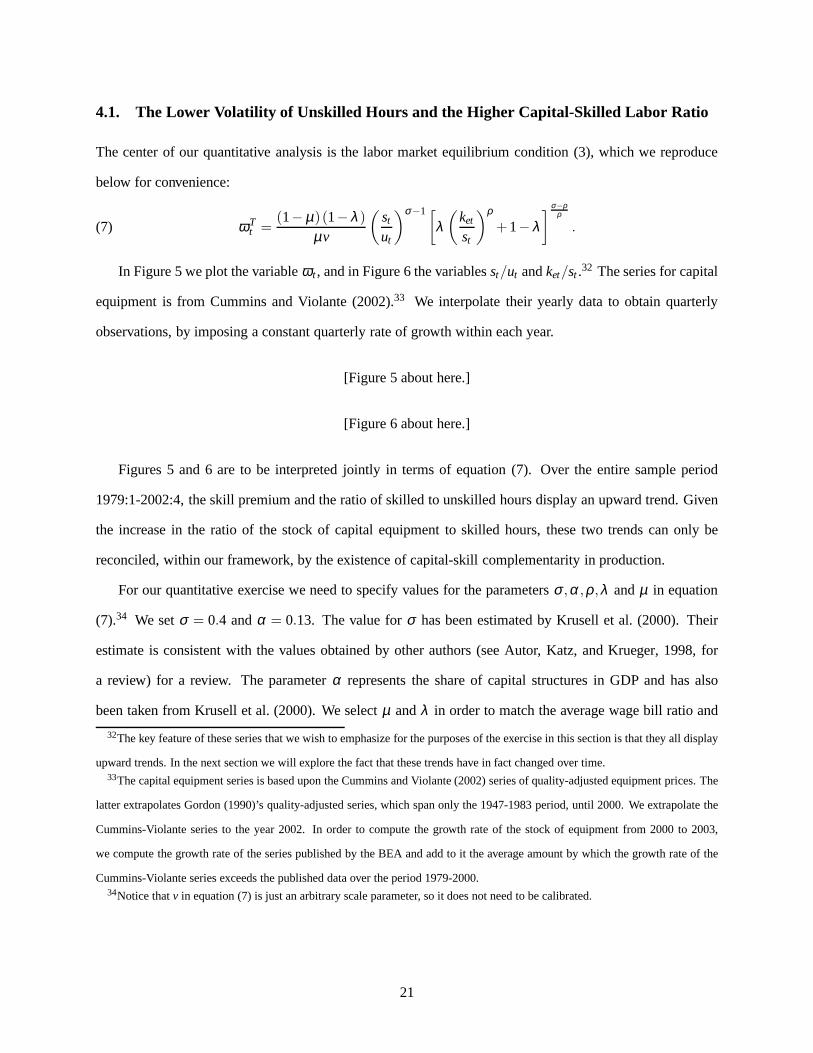
4.1. The Lower Volatility of Unskilled Hours and the Higher Capital-Skilled Labor Ratio

The center of our quantitative analysis is the labor market equilibrium condition (3), which we reproduce

below for convenience:

(7) ωTt =

(1−µ) (1−λ)

µv

(st

ut

)σ−1[λ

(ket

st

)ρ+1−λ

] σ−ρρ

.

In Figure 5 we plot the variableω t , and in Figure 6 the variablesst/ut andket/st .32 The series for capital

equipment is from Cummins and Violante (2002).33 We interpolate their yearly data to obtain quarterly

observations, by imposing a constant quarterly rate of growth within each year.

[Figure 5 about here.]

[Figure 6 about here.]

Figures 5 and 6 are to be interpreted jointly in terms of equation (7). Over the entire sample period

1979:1-2002:4, the skill premium and the ratio of skilled tounskilled hours display an upward trend. Given

the increase in the ratio of the stock of capital equipment toskilled hours, these two trends can only be

reconciled, within our framework, by the existence of capital-skill complementarity in production.

For our quantitative exercise we need to specify values for the parametersσ ,α ,ρ,λ andµ in equation

(7).34 We setσ = 0.4 andα = 0.13. The value forσ has been estimated by Krusell et al. (2000). Their

estimate is consistent with the values obtained by other authors (see Autor, Katz, and Krueger, 1998, for

a review) for a review. The parameterα represents the share of capital structures in GDP and has also

been taken from Krusell et al. (2000). We selectµ andλ in order to match the average wage bill ratio and

32The key feature of these series that we wish to emphasize for the purposes of the exercise in this section is that they all display

upward trends. In the next section we will explore the fact that these trends have in fact changed over time.33The capital equipment series is based upon the Cummins and Violante (2002) series of quality-adjusted equipment prices. The

latter extrapolates Gordon (1990)’s quality-adjusted series, which span only the 1947-1983 period, until 2000. We extrapolate the

Cummins-Violante series to the year 2002. In order to compute the growth rate of the stock of equipment from 2000 to 2003,

we compute the growth rate of the series published by the BEA and add to it the average amount by which the growth rate of the

Cummins-Violante series exceeds the published data over the period 1979-2000.34Notice thatv in equation (7) is just an arbitrary scale parameter, so it does not need to be calibrated.

21

aggregate labor share over the entire period 1979:1-2002:4.35 Unlike the case ofσ , estimates ofρ in the

literature tend to be more dispersed. We pick the substitution parameterρ in order to match the average

growth rate of the skill premium in the entire sample. Regarding the computation of the data moments, the

aggregate labor share of income is set at 0.70, consistentlywith NIPA data. In addition, we use the CPS data

to construct the average wage bill ratio and the average growth rate of the skill premium.

[Table 3 about here.]

Table 3 summarizes our calibration exercise under a constant production structure. It contains the values

of the calibrated parameters together with the data momentsthat they match.

To evaluate the performance of the model, we use the actual series forut , ket andωTt (computed as the

HP-filter trend ofω t ) together with the calibrated parameters (Table 3) in equation (7), to obtain a predicted

series ˆst for skilled hours. We then HP-filter ˆst to extract its cyclical component ˆsct . Figure 7 plots the actual

series forst together with ˆst . Figure 8 reports ˆsct , together with the the cyclical components of output and

actual total skilled hours.

[Figure 7 about here.]

[Figure 8 about here.]

Table 4 contains the cyclical properties of skilled hours predicted by our model, before and after 1984.

This is our “benchmark” exercise under constant parameters, when both effects considered in this section

are at work.

[Table 4 about here.]

In interpreting these results recall that, with no capital-skill complementarity in production (σ = ρ),

the ratio of the standard deviations of skilled and unskilled hours would equal one in both sub-periods.36

The existence of capital-skill complementarity in production, by itself, explains why the relative standard

deviation of skilled hours is significantly smaller than onebefore 1984.

35One has to worry about whether the skill premium predicted byequation (7) is invariant to the unit in which capital equipment

is measured. It turns out that this is indeed the case: it is relatively easy to show that different measurement units are fully absorbed

by the share parametersλ andµ in our calibration.36As a consequence, the volatility of skilled hours relative to GDP would also be approximately equal to one in both subperiods.

22

After 1984, the relative standard deviation of skilled hours increases by 17 percentage points (from 0.61

to 0.79), which is about a quarter of the increase observed inthe data. This change is due to the two effects

considered in this section. First, the absolute volatilityof the cyclical component of unskilled hours (uct ) has

declined dramatically after 1984, while the volatility of the cyclical component of capital equipment (kcet) did

not change in a significant way over the sample period. In the data,std(kcet)/std(uc

t ) increased from 0.50

before 1984:1 to 0.91 after this date. This fact in conjunction with capital-skill complementarity implies

that, as explained in Section 3, the volatility of skilled hours will drop proportionally less than the volatility

of unskilled hours and GDP. Second, the ratioket/st has increased over the sample period, especially in the

1990’s, when its growth rate more than doubled. Ifρ < 0, as in our benchmark calibration, this increase

should have increased the relative volatility of skilled hours.

In order to get a sense of the relative contribution of each ofthese two effects, we have performed a

simple experiment with equation (4). For given coefficientQ, and for given actual series for the cyclical

components of unskilled hours and capital equipment, this equation can be used to obtain a predicted series

for the cyclical component of skilled hours. We have computed the value of the coefficientQ such that the

predicted series for skilled hours displays a relative standard deviation for the period 1979:1-1983:4 equal

to the one predicted by the benchmark case (i.e., 0.61). The relative standard deviation of skilled hoursafter

1983:4 obtained using this procedure is reported in Table 4 under the label “Constantket/st after 1984”. This

figure, 0.76, represents the relative volatility of skilledhours in the sub-period following 1984, under the

assumption that the coefficientQ, and therefore the ratioket/st , stays constant at its pre-1984 value.37 This

result suggests that most of the increase in the relative volatility of skilled hours explained by the constant

parameter model can be attributed to the lower volatility ofunskilled hours over the business cycle.

4.2. The Decline in Capital-Skill Complementarity

In this section we evaluate the magnitude of the third mechanism described in Section 3. We have argued

that the increase in the relative volatility of skilled hours might be attributed, at least in part, to a reduction in

the degree of capital-skill complementarity in the economy. In what follows we first provide some empirical

evidence in favor of this hypothesis and discuss how the latter might be justified from a theoretical point of

view. We then evaluate its contribution to the cyclical behavior of skilled hours.

37Notice that a trend inke/s would induce a trend in the coefficientQ.

23

The decline in capital-skill complementarity. Our starting point is the observation that assuming a

constant set of parameters for the whole sample period (the benchmark case of the previous section) implies

that the model is not able to replicate the long-run behaviorof the skill premium, as Figure 9 suggests.

[Figure 9 about here.]

The principal reason for this failure is that the trends in the skill premium and the input ratios appear to

change sometime around the late 1980’s. Figure 5 shows a decline in the average growth rate of the skill

premium between the 1979:1-1989:3 and 1989:4-2002:4 sub-periods (the reason for splitting the sample

around 1989:4 for the purpose of looking at the long-run trends will become clear later in this section).

In the first sub-period, the skill premium has grown, on average, at a rate of 1.36 percent per year, while

in the second period it has grown at an average rate of 0.74 percent per year. Figure 6 depicts the evolution

of the relative inputsket/st andst/ut . This figure shows a substantial acceleration after 1989:3 in the growth

rate ofket/st (from 2.69 percent to 6.19 percent per year) and a contemporaneous slowdown in the growth

of st/ut (from 2.89 percent to 1.89 percent per year).38 These observations accord well with the empirical

evidence presented by Card and DiNardo (2002) and Beaudry and Green (2002), who also notice that the

skill premium has grown at a significantly smaller rate afterabout 1987 with respect to the previous seven

years, despite an acceleration in the growth rate of the stock of capital equipment.

The evolution ofket/st andst/ut since the late 1980’s represents a challenge to the view thatthe long-

run behavior of the skill premium in the 1980’s and 1990’s canbe explained using a production structure

characterized by capital-skill complementarity and constant parameters. The latter would have predicted a

faster, rather than a slower, increase in the skill premium since 1989, because the faster growth inket/st

and the slower growth inst/ut should have made skilled labor relatively more productive than in the first

sub-period (see also Figure 9). Instead, Figure 5 clearly tells otherwise.39

38The increase in the growth rate ofket/st can be traced back to a substantial decline in the relative price of equipment in

terms of consumption, brought about by a significant acceleration in the technological progress specific to the production of capital

equipment goods. In part as a consequence of this fact, investment in equipment has accelerated in the post-1989 period,and most

notably in the late 1990’s. This is consistent with anecdotal evidence suggesting that the 1990’s where a boom period in terms of

investment in equipment.39Figure 9 and Figure 7 are obviously closely related, as they are two different ways of conveying the same information. In the

constant production structure model, the sharp increase incapital equipment that took place during the 1990s induces asignificant

24

Our view is that this evidence may point to a reduction in the degree of complementarity in production

between skilled labor and capital equipment starting from the late 1980’s. The lower degree of capital-skill

complementarity would then contribute to explain the increase in the relative volatility of skilled hours over

the business cycle.

To evaluate the importance of this effect for the cyclical behavior of skilled hours, we follow a simple

approach, and assume a once-and-for-all decline inσ − ρ in the production function (1). We view this

modelling approach more as a convenient short-cut than a rigorous model of the underlying phenomena, as

we share economists’ reluctancy to base their theories on changes in “structural parameters” such asσ and

ρ. A full-fledged model should be able to capture the decline in capital-skill complementarity as a slowly-

evolving process spanning several years, presumably due tothe diffusion and routinization of computers

and information technologies, and reaching maturity around the late 1980’s. In this regard, Katz (1999)

(page 17) has interpreted the slowdown in the growth of the relative demand for skill since the late 1980’s,

as reflecting a “maturing of the computer revolution”, whereby “as technologies diffuse and become more

routinized the comparative advantage of the highly skilleddeclines.” Along the same line, Blanchard (2003)

(page 281) conjectures that “it is likely that computers will become easier and easier to use in the future, even

by low skill workers. Computers might even replace high-skill workers, those workers whose skills involve

primarily the ability to compute or to memorize.” The theoretical model that, perhaps, best captures this

view is the one developed by Greenwood and Yorokoglu (1997) to describe the effects of the faster decline

in the price of equipment since 1974 on the relative demand for skilled labor. In this model, a technological

revolution is followed by a transitory increase in the demand for skilled labor which is needed to implement

the new technologies. Afterwards, as the latter have been adopted and implemented, the relative demand

for skilled labor declines towards its original steady state level. While we agree that it would be more

satisfactory to use a version of Greenwood and Yorokoglu (1997) model as a foundation for our empirical

exercise, we do not pursue this route because of the difficulttask of augmenting the latter with business

cycle fluctuations.

Business cycle implications.In order to evaluate the importance of the evidence described above for the

increase in relative productivity of skilled labor, all else constant. Since the actuals/u ratio does not grow any faster in the 1990s,

this must lead to a faster growth in the predicted skill premium (Figure 9). Similarly, since the actual skill premium does not grow

any faster in the 1990s, this must lead to a faster growth in predicted skilled employment (Figure 7).

25

cyclical properties of skilled labor, we recalibrate the model allowing for a different degree of capital-skill

complementarity after a certain break date in the late 1980’s.

In order to set values for the model’s parameters and determine a precise break date, we proceed as

follows. First, for a given break dateT, we assume that while the parametersρ, µ andλ of the produc-

tion function (1) may take on different values before and after T, the parametersα andσ remain instead

unchanged over the entire sample period. The values ofρ , µ andλ for the sub-period precedingT are set

exactly as in Section 4.1, in order to match the average laborshare, the average wage bill ratio, and the

average growth rate of the skill premium between 1979:1 andT. The values ofρ , µ andλ for the sub-

period followingT are set in an analogous way. For given set of parameters, we then select the break date

T that minimizes the sum of squared errors between the trend inthe actual skill premium,ωT , and the skill

premium predicted by the model. This procedure yieldsT = 1989:3 as the break date.

[Table 5 about here.]

The results of this calibration exercise are summarized in Table 5. Notice, in particular, how the cali-

brated elasticity of substitution between skilled labor and capital equipment is now much lower before 1984,

and much higher after 1984, compared to the benchmark case ofTable 3.

Before proceeding, a few observations are in order. First, the assumption that the decline inσ − ρ

is due to an increase inρ , rather than a decrease inσ , is motivated by the idea that, as computers and

information technologies become more routinized, it is thedegree of complementarity of skilled labor with

capital equipment that might decline. This assumption turns out to be quite innocuous as similar results can

be obtained by keepingρ the same across sub-periods and lettingσ adjust. Second, after the break date, it

is necessary to changeµ andλ together withρ , in order to avoid jumps in the predicted series for the skill

premium and to guarantee that the model is consistent with the evidence on the average labor income shares

in both sub-periods. Third, our break date for the model’s parameters (1989:3) occurs a few years after the

date (1983:4) in which we break the data series to analyze their cyclical properties. While in a literal sense,

it would be more consistent to have these two dates closer to each other, it is unreasonable to interpret the

reduction in the volatility of GDP or in the degree of capital-skill complementarity as having occurred in

a specific quarter or even year. Instead, we think of both of these phenomena as processes occurring over

time. Our approach is aimed at capturing this change in a simple way.

26

[Figure 10 about here.]

Figure 10 plots the actual data series for the HP-trend in theskill premium, and the skill premium

predicted by the model. The key feature illustrated by this figure is the ability of the model to reproduce the

slowdown in the growth rate of the skill premium, in spite of the underlying behavior of the relative input

ratios.

Figure 11 plots the actual data series for skilled hoursst together with the series ˆst . The model appears

to provide a good description of the behavior of skilled hours, even at higher frequencies. The overall fit of

the model clearly improves compared to Figure 7. We then HP-filter st to extract its cyclical component ˆsct .

Figure 12 reports ˆsct , together with the the cyclical components of output and actual total skilled hours.

[Figure 11 about here.]

[Figure 12 about here.]

[Figure 13 about here.]

[Table 6 about here.]

Table 6 contains the cyclical properties of skilled hours predicted by our model and compares them

both with the data and with results of Section 4.1. This tableillustrates how the change in the degree of

capital-skill complementarity is quantitatively important. In particular, the fact that the degree of capital-skill

complementarity before 1984 is higher than in the benchmarkcalibration, allows this version of the model

to predict a lower relative volatility of skilled hours in the first sub-period (0.55 against 0.61). Similarly,

the higher degree of capital-skill complementarity in the 1990’s generates a larger increase in the relative

volatility of skilled hours. The latter is 0.95 in the version of the model with changing parameters against

0.79 in the model with constant parameters. Notice also thatthe model correctly predicts that skilled hours

are more volatile than unskilled hours after 1984 and less volatile before 1984.40

40In order to verify the robustness of our results, we have performed some sensitivity analysis on the substitution parameter ρ.

Specifically, we have kept the estimated value ofρ in the pre-1989:3 subperiod constant at−2.21, and changedρ in the second

subperiod in two alternative ways. In the first experiment, we setρ = 0 in the second subperiod. The relative volatility of skilled

labor predicted by the model increases from 0.95 to 1.03, while the contemporaneous correlation with GDP remains equal to 0.67.

In the second experiment we setρ = −0.8. This gives a relative volatility of 0.97 and a correlation with GDP equal to 0.69. We

interpret these findings as suggesting that the results of Table 6 are fairly robust to changes in the key parameterρ.

27

In summary, the three effects of Section 4.1 jointly accountfor almost sixty percent

((0.95−0.55)/(1.05−0.37)) of the increase in the relative standard deviation of skilled hours observed

in the data. Most of the explanatory power of the model comes from the change in the production func-

tion parameters (about 55 percent), followed by the declinein the relative standard deviation of unskilled

hours (about 37 percent), and the increase in the ratio of capital equipment relative to skilled hours (about 8

percent).41

5. Before 1979: Evidence From the March CPS

The quantitative results of Section 4.2 provide some support for the hypothesis that the higher volatility

of skilled labor observed in the 1990’s might be due in part toa decline in the degree of complementarity

between skills and capital equipment. As observed above, such a decline is consistent with the view, origi-

nally advanced by Nelson and Phelps (1966) and more recentlyby Greenwood and Yorokoglu (1997), that

skilled workers have a comparative advantage in implementing and adopting new technologies. According

to this interpretation, the “technological revolution” that started in the mid 1970’s, has been characterized

by a transition period of 10-15 years. During this transition period the demand for skilled labor accelerated,

leading to a fast-growing skill premium and to the acyclicality of skilled labor documented in Section 2.2.

After this transition period, starting from the late 1980’s, new technologies become more routinized leading

to a slowdown in the demand for skilled labor. This slowdown is reflected in the decline in the growth rate

of the skill premium and the higher cyclicality of skilled labor.

If this line of argument is correct, one should expect skilled labor to be relatively acyclicalonly during

periods of “technological revolutions”, such as the late 1970’s and early 1980’s. In order to evaluate this

prediction of our model, we need to provide some evidence regarding the cyclical behavior of skilled labor

41We have changed the calibration of the model to evaluate the sensitivity of the results to different values of the elasticity

parameterσ . We have found that, even varying the parameterσ beyond the boundaries suggested by the empirical evidence does

not improve the performance of the model. Notice that, givenour parsimonious parameterization,σ and the share of structures,

α, are the only parameters that can, in principle, be set exogenously. Reasonable variations in the latter also do not give rise to

noticeably different results from those of Table 6. While variations in the other, calibrated, parameters of the model,λ ,µ, andρ,

could possibly generate a better fit of the model at the cyclical frequency, they would also oblige us not to be able to capture some

of the low frequency variations in the data. Given the role played by the latter in disciplining our empirical exercise wedid not

pursue this avenue.

28

before 1979. Given that the CPS ORG data are available only since that date, we construct measures of the

aggregate skilled and unskilled labor inputs using annual data from the March CPS for the period 1963-2002.

The analysis of Section 2.2 reveals that most of the increasein the volatility of skilled labor since 1984

is due to a higher volatility of aggregate employment, as opposed to average hours. Thus, for simplicity, we

focus exclusively on the extensive margin.42 Aggregate skilled labor in a given year is measured, using the

March CPS survey, as the aggregate number of weeks worked by individuals with a college degree in that

year. Aggregate unskilled labor is defined analogously.43

[Figure 14 about here.]

[Figure 15 about here.]

Figure 14 represents the HP-filtered series for aggregate skilled and unskilled labor from the March

CPS, together with aggregate GDP.44 Two features of these data stand out. First, from 1979 onwards, the

cyclical properties of aggregate skilled labor measured using the March CPS data are very similar to the

ones obtained using the ORG data, and represented in Figure 2. In particular, aggregate skilled labor is

relatively acyclical in the 1980 and 1981-82 recessions, while it is significantly more volatile afterwards.

Second, and more important, the March CPS data reveal that inthe period between 1963 and 1975, skilled

labor tends to be roughly as cyclical as unskilled labor.45 In other words, the acyclicality of skilled labor is

a transitional phenomenon stretching from the mid-1970’s to the mid-1980’s. This point can be easily seen

42Before 1976, the March CPS survey only asks individuals how many weeks they have workedlast yearand how many hours

they have workedlast week. This presents a limitation in computing a measure of total hours based upon this sample before 1976.

Also for this reason we decided to concentrate on aggregate employment.43To make these data as comparable to the ORG ones in Section 2.2as possible, we use the same sample selection criteria

described in the Appendix.44We used a smoothing parameter of 6.25, as suggested by Ravn and Uhlig (2002) for annual data.45This fact requires further comment, as few of the authors cited in the Introduction (particularly Kydland, 1984 and Keane

and Prasad, 1993) had found skilled labor to be relatively acyclical in earlier studies. We attribute this apparent discrepancy to

the fact that these authors use microdata samples for the period 1970-1980 (Kydland) and 1966-1981 (Keane and Prasad) that

include information from both the “high volatility” subperiod 1963-1975 and from the “low volatility” subperiod 1976-1983.

Additionally, in order to compute measures of the cyclicality of skilled labor, these authors adopt a regression approach in which

the unemployment rate in one year is correlated with workers’ employment status in the same year. This method fails to account

for any leads and lags in the response of skilled labor to cyclical fluctuations in GDP in the 1963-1975 subperiod (see Figure 14).

29

by considering, in Figure 15, the rolling standard deviation for skilled and unskilled labor and GDP in the

1963-2002 period. The figure clearly suggests that in theearlier as well as in thelater parts of this long

sample, the volatility of skilled labor was about the same asthe volatility of unskilled labor and GDP. The

rolling standard deviation of skilled labor reaches a minimum in the mid-1970’s, indicating that the decade

1976-1985 was indeed characterized by the smallest degree of volatility for this variable.46 This observation

supports our interpretation of the observed reduction in the volatility of aggregate skilled hours from the

mid-1980’s.

6. Complementary Explanations

In this paper we have focused on the hypothesis that the increase in the relative volatility of skilled labor

since the mid-1980’s reflects the end of a decade-long transition period during which the demand for skilled

labor accelerated dramatically. Since our model can only account for about 60 percent of the observed

increase in this volatility, in this section we discuss a fewexplanations that are potentially complementary

to ours.

6.1. Adjustment Costs to Skilled Labor and Temporary vs. Permanent Shocks to GDP

In the simple model of Section 3 we have for simplicity abstracted from adjustment costs to employment.

However, starting from Oi (1962), economists have argued that adjustment costs to skilled labor play an

important role in explaining the high frequency dynamics ofskilled employment. Thus, faced with tempo-

rary cyclical reductions in productivity or product demand, employers would prefer to hoard skilled labor

in order not to dissipate costly training costs. Lower adjustment costs for unskilled workers, instead, would

make unskilled employment more sensitive to the business cycle.

Within this context, the increase in the volatility of skilled employment documented in Section 2.2

might reflect a change in the nature of business cycle fluctuations. According to this hypothesis, the shocks

underlying the recessions in the early part of our sample were temporary, whereas the last two recessions

were driven by more permanent shocks.

46The relative standard deviation of the HP-filtered measure of skilled labor for the subperiods 1963-1975, 1976-1983, 1984-

2002 is, respectively, 0.91, 0.45, 1.13. The relative standard deviation of unskilled labor in these three periods is, respectively, 0.98,

0.89, 0.69.

30

If a recession is perceived to be temporary, and if skilled workers have higher adjustment costs, firms

might respond to a cyclical downturn with temporary layoffsof unskilled workers, but leave their skilled

workers in place. If a recession is instead perceived to be more permanent, as this hypothesis would hold

was the case since the mid-1980’s, then firms would have less incentive to hoard skilled labor. This argument

could potentially explain why skilled employment has become relatively more volatile in recent years.

The key question is, of course, whether business cycles shocks have become more permanent in recent

years. While this is difficult to measure empirically, thereis at least some indirect evidence consistent

with this view. Figure 16 plots Bureau of Labor Statistics series representing the aggregate number of

unemployed workers and the number of unemployed workers dueto temporary layoffs. It is clear from the

figure that temporary layoffs tend to increase systematically during all NBER-defined recessions preceding

the 1990-91 one. In the last two recessions, instead, temporary layoffs did not increase substantially.47 One

may interpret this evidence as suggesting that business cycle shocks have become more permanent in recent

years, thus leading to less hoarding of skilled workers.

[Figure 16 about here.]

It is also worth asking whether this story can explain the whole pattern followed by the volatility of

skilled labor since the early 1960s, as described in Section5. In this dimension, the labor-hoarding story

does not appear able to explain the facts. According to the evidence on temporary layoffs just discussed,

before 1975 the cyclical volatility of skilled labor shouldhave been small relative to the volatility of unskilled

labor and GDP. This is because of labor hoarding of skilled workers by firms facing temporary business cycle

shocks - as evidenced by the importance of temporary layoffsin the 1969-70 and 1973-75 recessions. The

evidence of Section 5 does not support this hypothesis, however, as skilled labor was as cyclical as unskilled

labor before 1975.

6.2. Adjustment Costs to Skilled Labor and General Purpose Technology

Aggregate skilled labor might have become more cyclical because new technologies have reduced training

costs for skilled workers. Some have argued (see e.g. Bresnahan and Trajtenberg, 1995 and Aghion, Howitt,

and Violante, 2002) that information technologies aregeneral purpose technologies, in the sense that they

47Bleakley, Ferris, and Fuhrer (1999) present and discuss similar evidence.

31

have the potential of being widely used and applied in a variety of sectors of the economy. It follows that

skilled workers’ comparative advantage in using information technologies should translate into a greater

transferability of their skills across firms, jobs, and sectors of the economy. This lower specificity of work-

ers’ human capital would then entail lower training costs for firms and consequently reduce the extent of

labor hoarding in response to cyclical fluctuations. Skilled hours would then become more volatile over the

business cycle. Moreover, lower adjustment costs for skilled labor should also have implied an increase in

separation rates for this group of workers, relative to the unskilled group, since the mid 1980’s. A few papers

have indeed documented that this has been the case. For example, Rodriguez and Zavodny (2003) analyze

data from the Displaced Workers Surveys and document an increase in displacement rates for college edu-

cated workers between 1983-87 and 1993-97. Farber (2005) reports a similar trend comparing the 1980’s

with the 1990-2004 period.

Notice that this evidence is in principle also consistent with the capital-skill complementarity story

developed above. According to the latter, a lower degree of complementarity between skilled labor and

capital equipment in the 1990’s should have made skilled employment at the firm-level more sensitive to

aggregate as well as idiosyncratic shocks. In turn, this higher sensitivity would translate into higher cyclical

andaverageseparation rates for skilled workers.

We again ask whether this hypothesis might also explain the dynamics since the early 1960s. Notice that,

according to the general purpose technology story, skilledlabor should have beenlessvolatile than unskilled

labor even before 1975. This is because, before the information technology revolution, technologies were

such that the human capital of skilled workers was more “specific” to a particular employer and therefore

harder to transfer across jobs. Hence, this hypothesis doesnot appear to be able to account for the evidence

of Section 5.

6.3. Changes in Taxes

The US has experienced significant tax cuts in 1981 and 1986. These tax reforms also featured a marked

reduction in tax progressivity. As such, skilled workers were likely to have benefited the most from the tax

cuts. A natural question is whether this policy change mighthave contributed to the increase in the relative

volatility of skilled hours.

To address this issue, consider the situation where the economy moves into an expansion period char-

32

acterized by rising hourly wages. The extent to which skilled workers would be willing to expand their

working hours depends on the progressivity of the tax code. If marginal tax rates increase steeply with

income, one should expect skilled workers to increase theirlabor supply significantly less than unskilled

workers. As the tax code becomes less progressive, skilled workers should be willing to expand their labor

supply relatively more. Thus, in principle, a reduction in the progressivity of tax rates might account for

Stylized Fact #1.48 This mechanism, while plausible, runs into a problem: the evidence of Section 2.2 re-

veals that Stylized Fact #1 is mainly due to the higher cyclical volatility of skilledemploymentrather than of

average hours worked by employed individuals. It is an open question whether a decrease in the progressiv-

ity of the tax code would be able to explain the higher volatility of skilled employment. In addition to this

issue, it is also unclear how this mechanism could account for the relatively high volatility of skilled labor

in the 1960’s and early 1970’s (Section 5).

In summary, the purpose of this section has been to discuss some explanations for the higher volatility

of skilled labor, complementary to the one we have explored in this paper. Our main conclusion is that,

like our story, some of these explanations are indeed plausible in accounting for the increase in the relative

volatility of skilled labor. However, unlike our story, it is not clear whether they can provide a comprehensive

account of the observed dynamics of input quantities and prices since the early 1960’s, both at high and low

frequencies. Specifically, they appear, on the surface, inconsistent with the non-linear pattern followed by

the cyclical volatility of skilled labor during the last 40 years or so. More work is needed to develop and test

these other stories.

7. Summary and Conclusions

In recent years economists have devoted considerable attention to documenting and analyzing the increased

inequality between skilled and unskilled workers. The focus of the literature has been on the low-frequency

increase of the college premium. In this paper, we have studied another dimension along which skilled

and unskilled workers are traditionally thought to differ:the sensitivity of their employment status to the

business cycle. The data suggest that, while wage inequality between skilled and unskilled workers has been

48Notice that while the mechanisms reviewed in Sections 6.1 and 6.2 operate on labor demand, this one relies on cyclical

variations in the relative labor supply of skilled workers.

33

increasing over the last 25 years, inequality among these two groups, as measured by the sensitivity of their

employment status to business cycles, is instead lower now than it was 20 years ago. Rather than viewing

the low and the high-frequency dynamics of inequality as separate phenomena, our hypothesis is that the

technological factors responsible for the long-run evolution of wage inequality also help us to understand

the short-run dynamics of skilled and unskilled labor.

Using high-frequency CPS data for the period 1979:1-2003:4, we have documented a dramatic increase

in the cyclical volatility of aggregate skilled hours relative to GDP, starting from the mid-1980’s. Aggregate

skilled hours display little cyclicality in the 1980 and 1981-82 recessions relative to unskilled hours and GDP.

Starting from the mid-1980’s, instead, aggregate skilled hours become more volatile than both unskilled

hours and GDP. We have provided an interpretation of this evidence using a simple supply/demand model

for skilled and unskilled labor based on the hypothesis of capital-skill complementarity in production. In

particular, within this framework, we have considered the impact of the following three effects on the relative

volatility of skilled hours: a reduction in the absolute volatility of GDP and unskilled hours since 1984, an

increase in the level of capital equipment relative to skilled labor over the sample period, a reduction in the

degree of capital-skill complementarity since the late 1980’s. These three mechanisms can jointly explain

about sixty percent of the observed increase in the relativevolatility of skilled labor, with the reduction in

the degree of capital-skill complementarity playing the key role quantitatively.

In evaluating these results it is important to emphasize that the reduction in the degree of capital-skill

complementarity that we postulated involves a discrete change in one of the model’s structural parameters.

While this approach represents a convenient modelling short-cut, a rigorous investigation of this mechanism

should be based on a full-fledged general equilibrium model in which the complementarity between skilled

labor and capital equipment evolves endogenously over time.49 We leave this interesting, but non-trivial,

extension to future research.

A second open question concerns the evidence regarding the change in the degree of capital-skill com-

plementarity. In the paper we use the low-frequency information contained in the pre and post-1989 trends

in the skill premium to obtain an estimate of this change. While this procedure is consistent with the lit-

erature on the dynamics of the skill premium (e.g. Krusell etal., 2000), additional evidence on the matter

49As we discussed in the text, one option would be to adopt the framework developed by Greenwood and Yorokoglu (1997). See

also the papers by Acemoglu (1998) and Kiley (1999).

34

would certainly strengthen the paper’s results. We believemicro evidence on the labor market outcomes of

skilled individuals may prove to be particularly informative.

35

A. Appendix

A.1. Additional Information Regarding the Data

In this appendix we provide some additional information regarding the steps followed to construct the vari-

ables used in the paper.

Sample Selection

For each quarter, we restrict attention to individuals in the labor force that are not self-employed to con-

centrate on paid earnings. For individuals reporting to be employed, we use the following sample selection

criteria:

1. Eliminate those with either missing or zero reported earnings.

2. Assign actual hours worked last week to usual hours, if usual hours is missing. This addresses the

fact that individuals reporting “hours vary” are declared as having missing usual hours (but not actual

hours) after 1993, causing a slight discontinuity in the series for hours between 1993:4 and 1994:1. In

fact, it turns out that this imputation of usual hours is applicable only after 1994.

3. Eliminate those with either zero or a missing value for actual hours, and similarly for usual hours.

Demographic Groups

We partition the sample into 240 demographic groups in a way analogous to Katz and Murphy (1992)

and, more recently, Krusell et al. (2000). First, each individual is either male or female. Second, starting

from age 16, we create 10 five-year age groups. Third, we consider three race groups, whites, blacks,

and otherwise. Last, we create four education groups, (1) nohigh school diploma (less than 12 years

of completed schooling), (2) high school graduate (12 yearsof completed schooling), (3) some college

(between 13 and 15 years of completed schooling) and (4) college graduate and more (16 years of completed

schooling and above). After 1992, consistently with the CPSeducation classification change from years of

schooling to educational categories, education group (1) corresponds to less than a high school diploma, (2)

to a high school diploma, (3) to more than a high school degreebut less than a B.A., and (4) to a B.A. degree

36

or higher. This adjustment produces time-series for the number of individuals in each education group, as

well as for the various variables of interest, that display no significant break in 1992.

In defining skill groups, we assign education groups (1)-(3)to the unskilled category and education

group (4) to the skilled category.

Efficiency Units and Wages

A primary reason for recording demographic variables is to allow us to compute adjusted measures

of the aggregate labor input, in which actual hours are weighted by some time-invariant base wage rate.

This produces series for the labor input in efficiency units,which is more sensible for aggregation across

demographic groups. We again proceed in a way analogous to Katz and Murphy (1992) and Krusell et al.

(2000).50

First, for each quarter and for each demographic group in ourpartition we compute, for employed indi-

viduals, (i) the average hourly wage rate, (ii) the average weekly working hours, and (iii) the demographic

group’s weight in the population. Formally, and using Krusell et al. (2000)’s notation, letG be our popula-

tion partition, where each demographic group is indexed byg. We compute:

hg,t =∑i∈g µ i,thi,t

∑i∈g µ i,t,

wg,t =∑i∈g µ i,t (wi,thi,t)

∑i∈g µ i,thi,t

µg,t = ∑i∈g

µ i,t ,

wherewi,t andhi,t are, respectively, the individual’s real hourly wage and usual weekly hours, andµ i,t is the

individual’s population weight.

Following Kydland and Prescott (1993), we select the time average of the wage rates over the whole

sample as the weights to be placed on hours.51 Denoting these weights by ¯wg, for g∈ G, we compute the

50It may be useful at this point to relate our approach to that ofBowlus et al. (2002). These authors propose a methodology

for constructing labor input series in efficiency units which is based upon a human capital production function with time-varying

productivity parameters. Our approach, instead, implicitly assumes no technological progress (theβ ’s in Bowlus et al.’s (2002)

notation are constant). In reality, however, since our analysis filters out low frequency movements in the data, it is in fact consistent

with long-run technical change.51We note that, since some demographic groups have no observations in some quarters, the number of observations used to

37

average labor input for a particular population categoryj ∈ G j as:

Nj,t = ∑g∈G j

µg,t wghg,t .

Depending on the question being asked in the main body of the paper,G j may correspond, for instance,

to skilled individuals, or to skilled individuals working in a particular sector, or having a certain occupation.

Similarly, the average wage rate for subgroupG j is computed as the ratio between total weekly earnings

and adjusted weekly hours:

Wj,t =∑g∈G j

µg,twg,thg,t

Nj,t.

This provides a real hourly wage rate per unit of efficiency supplied by groupj individuals.52

Sectors and Occupations

For the analysis by sector of activity, we use the NBER-created 2-digit industry codes (variable “dind”)

and assign them to the 1-digit 1987 SIC categories (with manufacturing split into durable and non-durable

manufacturing).

For the analysis by occupation, one major difficulty is that our data does not provide a time-consistent

occupational classification. Until 1982 it is based on the 1970 Census, but from 1983 until 2002 it is based

on the 1980 Census. We developed an assignment between 2-digit occupational codes (and when necessary

3-digit codes) and 1-digit codes. Using this assignment, wedo not observe any break in the number of

people in each occupational category from 1982 to 1983. The assignment rule is available upon request.

A.2. Controlling for Composition Effects

In this appendix we analyze the MORG data at lower levels of aggregation and report the results regarding

the robustness of our stylized facts to possible composition effects.

compute average wages may differ from group to group. Also, similar results obtain if the weights were based on any particular

base-period wages.52Our analysis implicitly assumes two separate markets for skilled and unskilled workers, each type earning a different wage per

efficiency unit of labor supplied.

38

A.2.1. Sectoral Composition

In order to address composition effects due to the sectoral composition of the workforce, we computed the

sectoral distribution of total hours worked by skill group and the business cycle statistics of total hours by

one digit sector and skill group.53 These are reported in Table 7. In the “Relative Volatility” columns, we

report in parenthesis the ratio of post to pre-1984 relativestandard deviations.54

[Table 7 about here.]

As Table 7 suggests, in many service industries (see for example the row “Various Service Industries,”

which includes Business and Repair Services, Personal Services, Entertainment and Recreational Services,

and Professional and Related Services) the volatility of aggregate hours has increased for both skilled and

unskilled workers, even if proportionally more for skilledworkers. Moreover, within the manufacturing

sector the relative volatility of skilled hours has also increased significantly while the relative volatility of

unskilled hours has remained approximately constant (as indurables) or increased proportionally less (as

in nondurables).55 This indicates that our results are not due to differences inthe sectoral composition of

employment across skilled and unskilled individuals.

53For the analysis by sectors and occupation, one major difficulty is that our data does not provide a consistent occupational

classification over time. Until 1982, it is based on the 1970 Census, but from 1983 until 2002 it is based on the 1980 Census.To

overcome this problem, we have developed an assignment between 2-digit occupational codes (and when necessary 3-digitcodes)

and 1-digit codes. Using this assignment we do not observe any break in the number of people in each 1-digit occupational category

from 1982 to 1983. Notice that our analysis by sectors and occupations is restricted to 1979:1-2002:4 because, from 2003onwards,

the CPS uses yet a different classification system, based upon the 2000 Census.54The statistics on employment and working hours per employedworkers are available from the authors upon request. As already

observed in Section 2.2 for the broad aggregates, most of thechange across the two subperiods is accounted for by changesin the

behavior of employment.55In interpreting these disaggregated results, and those of the following subsections, it is worth to keep in mind two issues.

First, one should naturally expect the labor aggregates in agiven sector (or occupation, as in the next subsection) to display larger

volatility than in the aggregate, simply as a result of sectoral idiosyncratic variations that tend to cancel out in the aggregate. The

second issue is that the more disaggregated labor inputs have to be computed with a relatively small number of observations.

Consequently, some of these disaggregated series are relatively noisy. For the same reason, since the number of observations

differs across sectors, comparing the cyclical behavior oflabor aggregates across sectors becomes potentially problematic. Thus,

in order to try to minimize the effects of this small-sample problem, we prefer to focus on thechangesacross periods in the relative

volatilities of the various labor market aggregates in a given sector.

39

As described in Section 2.3, in order to control more formally for these differences, we recomputed

the aggregate statistics of Table 1 by imposing that the share of aggregate skilled hours worked in each

industry is equal to the analogous share for unskilled hours. To do so, we exploited the fact that the cyclical

component of aggregate skilled and unskilled hours, denoted by st andut , can be expressed (approximately)

as the weighted average of the cyclical componentssjt andu j

t of industries’ hours, where the weightsκ jst and

κ jut are equal to the share of total hours worked in industryj in periodt:56

st ≈10

∑j=1

κ jsts

jt ,(8)

ut ≈10

∑j=1

κ jutu

jt .(9)

Our experiment consists of constructing a new measure of skilled hours, denoted bysut , which is char-

acterized by the same sectoral distribution as unskilled hours:

sut ≡

10

∑j=1

κ juts

jt .

[Table 8 about here.]

Table 8 reports the cyclical properties ofsut . This table reveals that imposing the same distribution of

skilled and unskilled hours across sectors tends to make theformer more volatile in both sub-periods. The

relative volatilities ofsut and st in the second sub-period exceed the ones in the first sub-period by a factor

of, respectively, 2.41 and 2.81.57 We conclude that, even after controlling for differences inthe composition

of hours across sectors, there has been a significant increase in the relative volatility of skilled hours since

1984.56As a way of checking the validity of this approximation, we have recomputed the moments of Table 1 using the right-hand

side of equations (8) and (9) as our measure of the cyclical component of skilled and unskilled hours, obtaining basically the same

results as in that table.57A related question is whether the increased volatility of skilled hours is due to an increase in their variances at the sectoral level,

or in their covariances. Decomposing the increase in the variance of total skilled hours relative to GDP into these two components

reveals that approximately 70 percent of this increase is due to higher sectoral variances and the remaining 30 percent to higher

sectoral covariances.

40

A.2.2. Occupational Composition

Table 9 displays the volatility and comovement with aggregate GDP of total hours by skill group and one-

digit occupation. We comment on this Table in the main text (Section 2.3).

[Table 9 about here.]

A.2.3. Males vs. Females

Table 10 represents the counterpart of Table 1 for the sub-sample of white males workers aged 31 to 55.58

We comment on this Table in the main text (Section 2.3).

[Table 10 about here.]

A.2.4. Skills vs. Education

Table 11 reports the main statistics regarding skilled and unskilled hours when we label a worker skilled if

he or she has a master, instead of a college, degree.59 We comment on this Table in the main text (Section

2.3).

[Table 11 about here.]

A.3. Canadian Data

Using Canadian household survey data from the Labour Force Survey (LFS) we have constructed time series

of employment for the period 1976:1-2002:4. For simplicity, in this case we just focus on employment since

most of the cyclical variation in total hours can be attributed to this margin. To construct these times series,

we applied the same sample selection criterion used for the CPS. We focused on individuals aged between

15 and 64 years that reported to be employed and at work, as either private or public employees. Skilled

individuals are those classified by the LFS as having a university degree before 1990, and those classified as

being university graduates after 1990. This difference reflects a change in the educational classification that

was implemented by the LFS starting in 1990. Unfortunately,the post-1990 classification is more restrictive

58The associated results for wages and the skill premium are available from the authors upon request.59The associated results for wages and the skill premium are available from the authors upon request.

41

(excludes university certificates), and this induces an artificial drop in the number of skilled individuals from

December 1989 to January 1990. We dealt with this issue by applying a constant multiplicative adjustment

factor to the whole pre-1990 series such that the number of skilled employed in December 1989 equalled

the one in January 1990. The workers in excess were added to the unskilled series before 1990. The raw

series were aggregated by quarters, and deseasonalized andnoise-filtered as described in the beginning of

Section 2.2.

Table 12 presents the cyclical properties of employment in Canada for the pre and post 1984:1 sub-

samples.

[Table 12 about here.]

These results reveal a dramatic increase in the volatility and comovement of aggregate employment for

college educated workers in Canada after 1984. The cyclicalproperties of unskilled employment, instead,

remain roughly constant in the two sub-periods. This is the same pattern found in the CPS data.60

60One noteworthy difference between the statistics of Table 12 and those of Table 1 is that, differently from the U.S., the relative

volatility of skilled employment in Canada is closer to thatof unskilled employment before 1984.

42

References

Acemoglu, Daron. “Why Do New Technologies Complement Skills? Directed Technical Change And Wage

Inequality,” TheQuarterlyJournalof Economics 113 (1998): 1055–1089.

Acemoglu, Daron. “Technical Change, Inequality, and the Labor Market,” Journalof EconomicLiterature

40 (2002), 7–72.

Aghion, Phillipe, Peter Howitt, and Gianluca Violante. “General Purpose Technology and Wage Inequality,”

Journalof EconomicGrowth 7 (2002), 315–345.

Autor, David H., Lawrence F. Katz, and Alan B. Krueger. “Computing Inequality: Have Computers Changed

the Labor Market?”QuarterlyJournalof Economics 113 (1998), 1169–1213.

Beaudry, Paul and David A. Green. “Changes in US wages 1976-2000: Ongoing Skill Bias or Major

Technological Change?” mimeo, University of British Columbia, October 2002.

Bils, Mark J. “Real Wages over the Business Cycle: Evidence from Panel Data,” Journalof Political

Economy 93 (1985), 666–689.

Blanchard, Olivier J.Macroeconomics. third edition. Prentice Hall, 2003.

Bleakley, Hoyt, Ann E. Ferris, and Jeffrey C. Fuhrer. “New Data on Worker Flows During Business Cycles,”

NewEnglandEconomicReview (1999), 49–76.

Bowlus, Audra, Haoming Liu, and Chris Robinson. “Business Cycle Models, Aggregation, and Real Wage

Cyclicality,” Journalof LaborEconomics 20 (2002), 308–335.

Bresnahan, Timothy F. and M. Trajtenberg. “General PurposeTechnologies ’Engines of growth’?”Journal

of Econometrics 65 (1995), 83–108.

Card, David and John E. DiNardo. “Skill-Biased Technological Change and Rising Wage Inequality: Some

Problems and Puzzles,”Journalof LaborEconomics 20 (2002), 733–783.

Chang, Yongsung. “Wages, business cycles, and comparativeadvantage,”Journalof MonetaryEconomics

46 (2000), 143–171.

43

Cummins, Jason G. and Giovanni L. Violante. “Investment-Specific Technical Change in the United States

(1947-2000): Measurement and Macroeconomic Consequences,” Review of EconomicDynamics 5

(2002), 243–284.

Fallon, P. R. and P. R. G. Layard. “Capital-Skill Complementarity, Income Distribution and Output Accou-

ting,” Journalof Political Economy 83 (1975), 279–302.

Farber, Henry S. “What Do We Know About Job Loss in the United States? Evidence from the Displaced

Workers Survey, 1984-2004,” Working Paper # 498, Industrial Relations Section, Princeton University,

January 2005.

Gordon, Robert J.TheMeasurementof DurableGoodsPrices. Chicago, IL: University of Chicago Press,

1990.

Greenwood, Jeremy and Mehmet Yorokoglu. “1974,”Carnegie-RochesterConferenceSerieson Public

Policy 46 (1997), 49–95.

Hansen, Gary D. “Indivisible Labor and the Business Cycle,”Journalof MonetaryEconomics 16 (1985),

309–327.

Hansen, Gary D. “The Cyclical and Secular Behaviour of the Labour Input: Comparing Efficiency Units

and Hours Worked,”Journalof Applied Econometrics 8 (1993), 71–80.

Katz, Lawrence F. “Technological Change, Computerization, and the Wage Structure,” mimeo, Harvard

University, September 1999.

Katz, Lawrence F. and Kevin M. Murphy. “Changes in Relative Wages, 1963-1987: Supply and Demand

Factors,”QuarterlyJournalof Economics 107 (1992), 35–78.

Keane, Michael P. and Eswar S. Prasad. “The Relation BetweenSkill Levels and the Cyclical Variability of

Employment, Hours and Wages,” Working paper 93/44, International Monetary Fund, May 1993.

Kiley, Michael T. “The Supply of Skilled Labour and Skill-Biased Technological Progress,”Economic

Journal 109 (1999): 708–24.

44

Kocherlakota, Narayana R. “The Equity Premium: It’s Still aPuzzle,” Journalof EconomicLiterature 34

(1996), 42–71.

Krueger, Alan B. 2002 “As recovery builds, the less educatedgo to the end of the employment line,”New

York Times, March 7.

Krugman, Paul. 1996 “White Collars Turn Blue,”NewYork Times, September 29.

Krusell, Per, Lee Ohanian, Jose-Vıctor Rıos-Rull, and Giovanni L. Violante. “Capital-Skill Complementar-

ity and Inequality: A Macroeconomic Analysis,”Econometrica 68 (2000), 1029–1053.

Kydland, Finn E. “Labor-Force Heterogeneity and the Business Cycle,” CarnegieRochesterConference

SeriesonPublicPolicy 21 (1984), 173–208.

Kydland, Finn E. and Edward C. Prescott. “Cyclical Movements of the Labor Input and its Implicit Real

Wage,” FederalReserveBankof ClevelandEconomicReview 29 (1993), 12–23.

Lindquist, Matthew. “Capital-Skill Complementarity and Inequality over the Business Cycle,”Reviewof

EconomicDynamics 7 (2004), 519–540.

McConnell, Margaret M. and Gabriel Perez-Quiros. “Output Fluctuations in the United States: What Has

Changed Since the Early 1980’s?”AmericanEconomicReview 90 (2000), 1464–1476.

Nelson, Richard R. and Edmund S. Phelps. “Investment in Humans, Technology Diffusion and Economic

Growth,” AmericanEconomicReviewPapersandProceedings 56 (1966), 69–75.

Oi, Walter. “Labor as a Quasi-Fixed Factor,”Journalof Political Economy 70 (1962), 538–555.

Prasad, Eswar. “Skill Heterogeneity and the Business Cycle,” CanadianJournalof Economics 29 (1996),

910–929.

Prescott, Edward C. “Why Do Americans Work So Much More than Europeans?” QuarterlyReview 28

(2004), 2–13.

Ravn, Morten and Harald Uhlig. “On Adjusting the HP-Filter for the Frequency of Observations,”Review

of EconomicsandStatistics 84 (2002), 371–376.

45

Reder, M. W. “The Theory of Occupational Wage Differentials,” AmericanEconomicReview 45 (1955),

833–852.

Rodriguez, Daniel and Madeline Zavodny. “Changes in the Ageand Education Profile of Displacement,”

IndustrialandLaborRelationsReview 56 (2003), 498–510.

Rogerson, Richard. “Indivisible Labor, Lotteries and Equilibrium,” Journalof MonetaryEconomics 21

(1988), 3–16.

Rosen, Sherwin. “Short-Run Employment Variation on Class-I Railroads in the U.S., 1947-1963,”

Econometrica 36 (1968), 511–529.

Solon, Gary, Robert Barski, and Jonathan A. Parker. “Measuring the cyclicality of real wages: how important

is composition bias?”QuarterlyJournalof Economics 109 (1994), 1–25.

Stock, James H. and Mark W. Watson. “Has the Business Cycle Changed and Why?” NBER

MacroeconomicsAnnual. MIT–Press, 2002, 159–218.

Young, Eric R. “The Wage Premium: A Puzzle,” mimeo, Florida State University, October 2003.

46

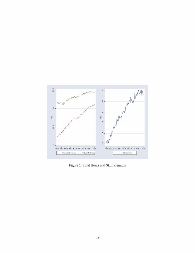
1919

.520

20.5

log

79:1 82:1 85:1 88:1 91:1 94:1 97:1 0:1 3:4

Total unskilled hours Total skilled hours

−.1

5−

.1−

.05

0.0

5.1

log

79:1 82:1 85:1 88:1 91:1 94:1 97:1 0:1 3:4

Skill premium

Figure 1: Total Hours and Skill Premium

47

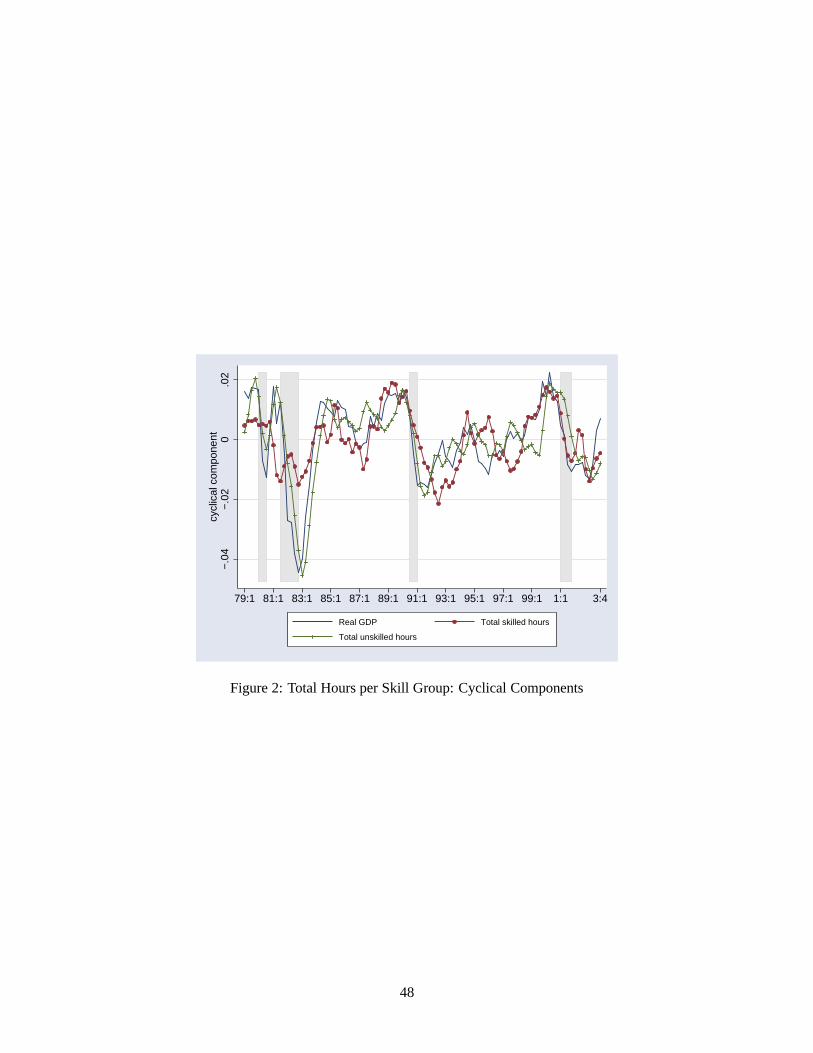
−.0

4−

.02

0.0

2cy

clic

al c

ompo

nent

79:1 81:1 83:1 85:1 87:1 89:1 91:1 93:1 95:1 97:1 99:1 1:1 3:4

Real GDP Total skilled hours

Total unskilled hours

Figure 2: Total Hours per Skill Group: Cyclical Components

48

.006

.008

.01

.012

.014

.016

79:1 82:3 86:1 89:3 93:1year:quarter

unskilled real GDPskilled

Figure 3: Rolling Standard Deviations (40 quarters ahead) of GDP, Unskilled and Skilled Hours

49

ωct

sct /uc

t

RS

RD

RDexpansion(↓ kcet/sc

t )

RDrecession(↑ kcet/sc

t )

Figure 4: Capital-Skill Complementarity and the Business Cycle

50

0.0

5.1

.15

.2.2

5

79:1 82:1 85:1 88:1 91:1 94:1 97:1 0:1 2:4year:quarter

Skill Premium 1.36% (before 1989:4)0.74% (after 1989:4)

Figure 5: Skill premium

51

0.5

11.

25

79:1 82:1 85:1 88:1 91:1 94:1 97:1 0:1 2:4year:quarter

Equipment/Skill Ratio Skilled/Unskilled Total Hours2.69% (before 1989:3) 2.89% (before 1989:3)6.19% (after 1989:4) 1.89% (after 1989:4)

Figure 6: Equipment-Skill and Skilled-Unskilled Input Ratios

52

.2.4

.6.8

1

79:1 82:1 85:1 88:1 91:1 94:1 97:1 0:1 2:4year:quarter

data model

Figure 7: Model Fit for the Total Skilled Hours under Constant Parameters

53

−.0

4−

.02

0.0

2cy

clic

al c

ompo

nent

79:1 81:1 83:1 85:1 87:1 89:1 91:1 93:1 95:1 97:1 99:1 1:1 2:4

Total skilled hours (data) Real GDP

Total skilled hours (model)

Figure 8: Model Performance under Constant Parameters: Cyclical Components

54

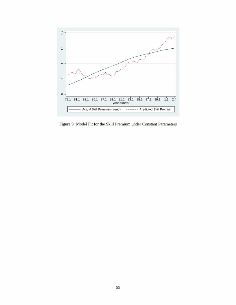
.8.9

11.

11.

2

79:1 81:1 83:1 85:1 87:1 89:1 91:1 93:1 95:1 97:1 99:1 1:1 2:4year:quarter

Actual Skill Premium (trend) Predicted Skill Premium

Figure 9: Model Fit for the Skill Premium under Constant Parameters

55

.8.9

11.

1

79:1 81:1 83:1 85:1 87:1 89:1 91:1 93:1 95:1 97:1 99:1 1:1 2:4year:quarter

Actual Skill Premium (trend) Predicted Skill Premium

Figure 10: Model Fit for the Skill Premium under Changing Parameters

56

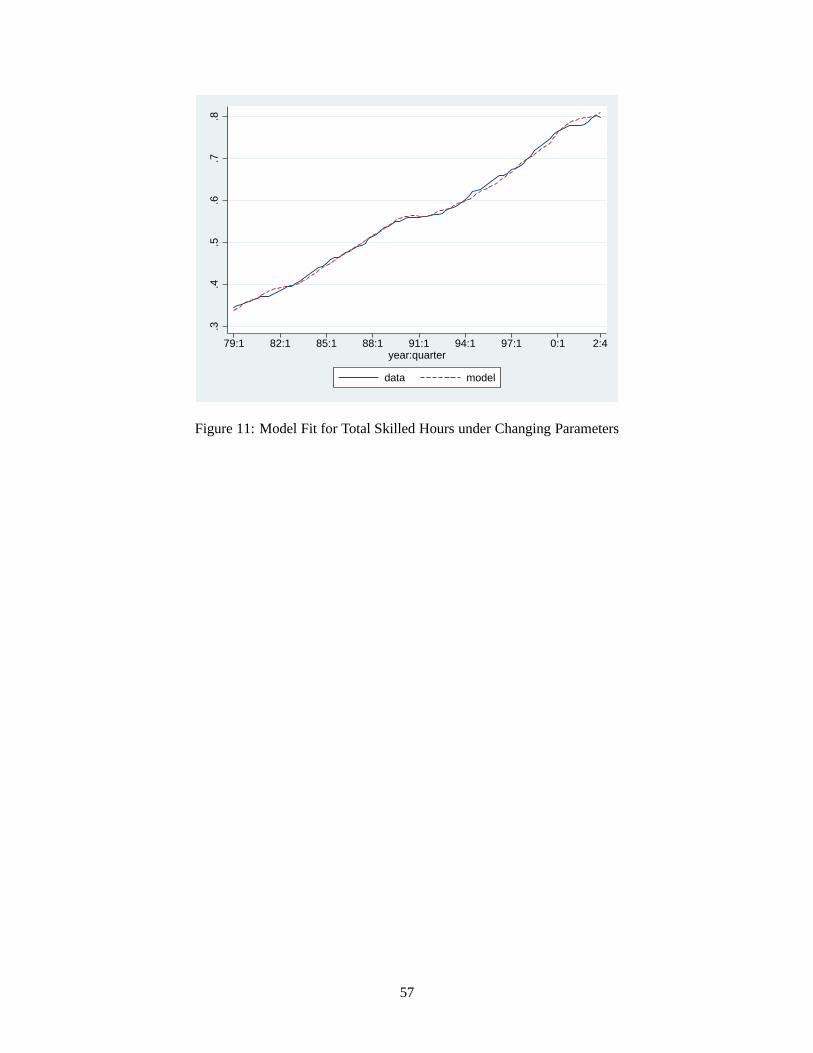
.3.4

.5.6

.7.8

79:1 82:1 85:1 88:1 91:1 94:1 97:1 0:1 2:4year:quarter

data model

Figure 11: Model Fit for Total Skilled Hours under Changing Parameters

57

−.0

4−

.02

0.0

2cy

clic

al c

ompo

nent

79:1 81:1 83:1 85:1 87:1 89:1 91:1 93:1 95:1 97:1 99:1 1:1 2:4

Total skilled hours (data) Real GDP

Total skilled hours (model)

Figure 12: Model Performance under Changing Parameters: Cyclical Components

58

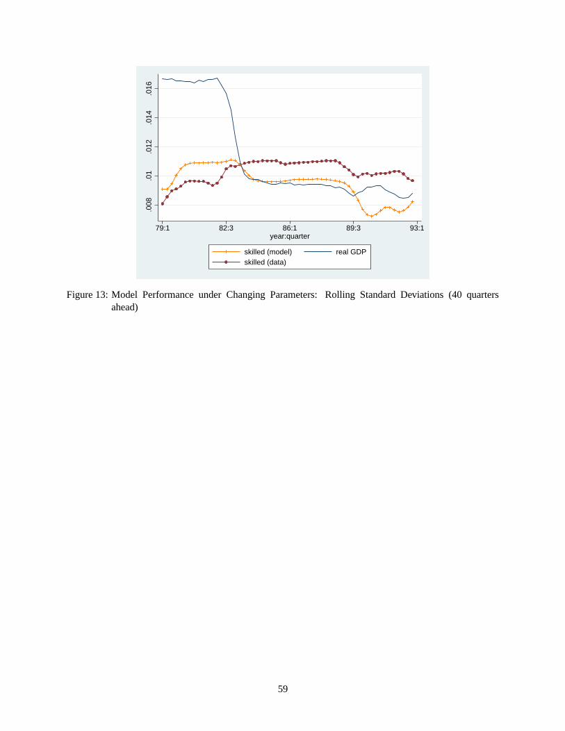
.008

.01

.012

.014

.016

79:1 82:3 86:1 89:3 93:1year:quarter

skilled (model) real GDPskilled (data)

Figure 13: Model Performance under Changing Parameters: Rolling Standard Deviations (40 quartersahead)

59

−.0

6−

.04

−.0

20

.02

.04

cycl

ical

com

pone

nt

1963 1967 1971 1975 1979 1983 1987 1991 1995 1999 2003

Total unskilled hours Real GDP

Total skilled hours

Figure 14: Cyclical Behavior of GDP, Skilled and Unskilled Employment - March CPS

60

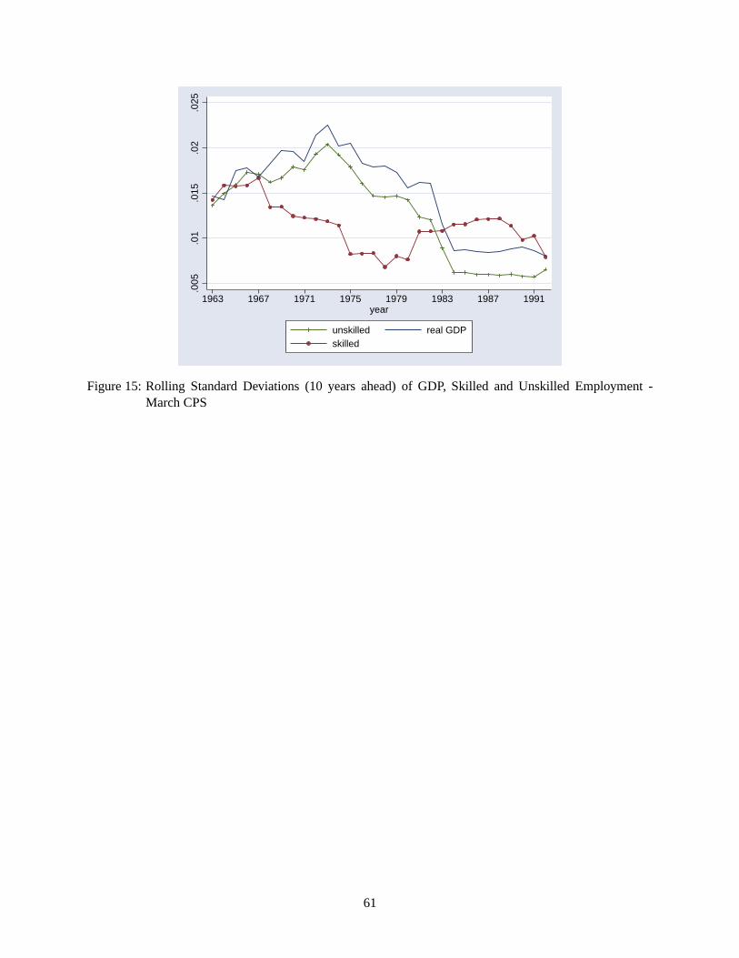
.005

.01

.015

.02

.025

1963 1967 1971 1975 1979 1983 1987 1991year

unskilled real GDPskilled

Figure 15: Rolling Standard Deviations (10 years ahead) of GDP, Skilled and Unskilled Employment -March CPS

61

020

0040

0060

0080

00th

ousa

nds

67:2 70:1 73:1 76:1 79:1 82:1 85:1 88:1 91:1 94:1 97:1 0:1 3:1 5:2

Job losers on temporary layoff Total job losers

Figure 16: Unemployed Persons by Reason, 1967-2005

62

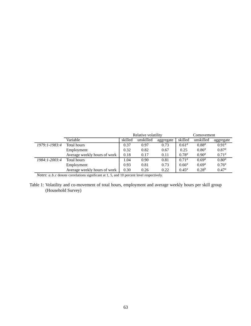
Relative volatility ComovementVariable skilled unskilled aggregate skilled unskilled aggregate

1979:1-1983:4 Total hours 0.37 0.97 0.73 0.61a 0.88a 0.91a

Employment 0.32 0.82 0.67 0.25 0.86a 0.87a

Average weekly hours of work 0.18 0.17 0.11 0.78a 0.90a 0.71a

1984:1-2003:4 Total hours 1.04 0.90 0.81 0.71a 0.69a 0.80a

Employment 0.93 0.81 0.73 0.66a 0.69a 0.76a

Average weekly hours of work 0.30 0.26 0.22 0.45a 0.28b 0.47a

Notes: a,b,c denote correlations significant at 1, 5, and 10 percent levelrespectively.

Table 1: Volatility and co-movement of total hours, employment and average weekly hours per skill group(Household Survey)

63

Relative volatility ComovementVariable skilled unskilled aggregate skilled unskilled aggregate

1979:1-1983:4 Hourly wage 0.75 0.57 0.63 0.29 0.41c 0.41c

Skill premium 0.26 -0.111984:1-2003:4 Hourly wage 0.96 0.66 0.74 0.35a 0.27b 0.29a

Skill premium 0.60 0.15Notes: a,b,c denote correlations significant at 1, 5, and 10 percent levelrespectively.

Table 2: Volatility and co-movement of the skill premium andwages per skill group and in the aggregate(Household Survey)

64

Period Parameters Values Target Moments Values1979:1-2003:4 λ 0.73 Average labor share in GDP 0.70

µ 0.54 Average wage bill ratio 0.56ρ -0.88 Average yearly growth rate of skill premium 1.06%

Table 3: Calibration under Constant Parameters

65

Relative volatility ComovementTotal Hours skilled unskilled skilled unskilled

1979:1-1983:4 Data 0.37 0.97 0.61 0.88Benchmark 0.61 0.63

1984:1-2002:4 Data 1.05 0.91 0.73 0.74Benchmark 0.79 0.69Constantket/st after 1984 0.76 0.69

Table 4: Quantitative Results under Constant Parameters

66

Period Parameters Values Target Moments Values1979:1-1989:3 λ 1 0.92 Average labor share in GDP 0.70

µ1 0.57 Average wage bill ratio 0.45ρ1 -2.21 Average yearly growth rate of skill premium 1.36%

1989:4-2002:4 λ 2 0.56 Average labor share in GDP 0.70µ2 0.52 Average wage bill ratio 0.65ρ2 -0.40 Average yearly growth rate of skill premium 0.74%

Table 5: Calibration under Changing Parameters

67

Relative volatility ComovementTotal Hours skilled unskilled skilled unskilled

1979:1-1983:4 Data 0.37 0.97 0.61 0.88Constant Parameters 0.61 0.63Changing Parameters 0.55 0.46

1984:1-2002:4 Data 1.05 0.91 0.73 0.74Constant Parameters 0.79 0.69Changing Parameters 0.95 0.67

Table 6: Quantitative Results: effect of changing capital-skill complementarity

68

Hours’ share (%) Relative Volatility ComovementTotal hours in skilled unskilled skilled unskilled skilled unskilled

1979:1-1983:4 Aggregate 100 100 0.37 0.97 0.61a 0.88a

Agriculture, Forestry and Fisheries 0.67 1.77 2.54 1.18 0.03 -0.14Mining 1.06 1.28 2.88 3.98 0.26 0.17Construction 2.13 6.83 3.10 2.22 0.59a 0.93a

Manufacturing - durables 11.21 17.36 1.12 1.93 0.67a 0.84a

Manufacturing - nondurables 6.66 10.57 1.22 0.94 0.14 0.84a

Transportation, Communications 4.94 9.26 1.29 1.14 0.37c 0.89a

Wholesale and Retail Trade 10.13 19.74 1.11 0.77 -0.22 0.82a

Finance, Insurance and Real Estate7.64 5.61 1.13 0.76 0.07 0.74a

Various Service Industries 47.30 21.27 0.27 0.58 0.39b 0.79a

Public Administration 8.30 6.41 1.22 2.55 0.38b -0.141984:1-2002:4 Aggregate 100 100 1.04 (2.81) 0.90 (0.93) 0.71a 0.69a

Agriculture, Forestry and Fisheries 0.59 1.75 9.20 (3.62) 3.73 (3.14) 0.17 0.07Mining 0.66 0.80 12.30 (4.26) 5.22 (1.31) 0.03 0.03Construction 2.12 7.63 5.52 (1.78) 3.20 (1.44) 0.42a 0.66a

Manufacturing - durables 9.73 13.65 3.42 (3.06) 2.09 (1.09) 0.42a 0.66a

Manufacturing - nondurables 5.77 8.56 2.84 (2.32) 1.72 (1.83) -0.04 0.42a

Transportation, Communications 6.14 9.68 2.87 (2.23) 1.66 (1.46) 0.38a 0.52a

Wholesale and Retail Trade 10.51 21.19 1.73 (1.56) 1.26 (1.63) 0.13 0.33b

Finance, Insurance and Real Estate8.76 5.65 2.84 (2.51) 2.24 (2.93) 0.33a 0.32a

Various Service Industries 47.88 25.79 1.15 (4.22) 0.78 (1.33) 0.58a 0.34a

Public Administration 7.89 5.31 3.37 (2.73) 2.57 (1.01) 0.30a -0.03Notes: Hours’ share is the average ratio of of total hours in a particular occupation relative to the aggregate. The numbers in parenthesisare the ratio of post to pre 1984 relative standard deviations. a,b,c denote correlations significant at 1, 5, and 10 percent levelrespectively.

Table 7: Volatility and co-movement of total hours per skillgroup, 1-digit industry (Household Survey).

69

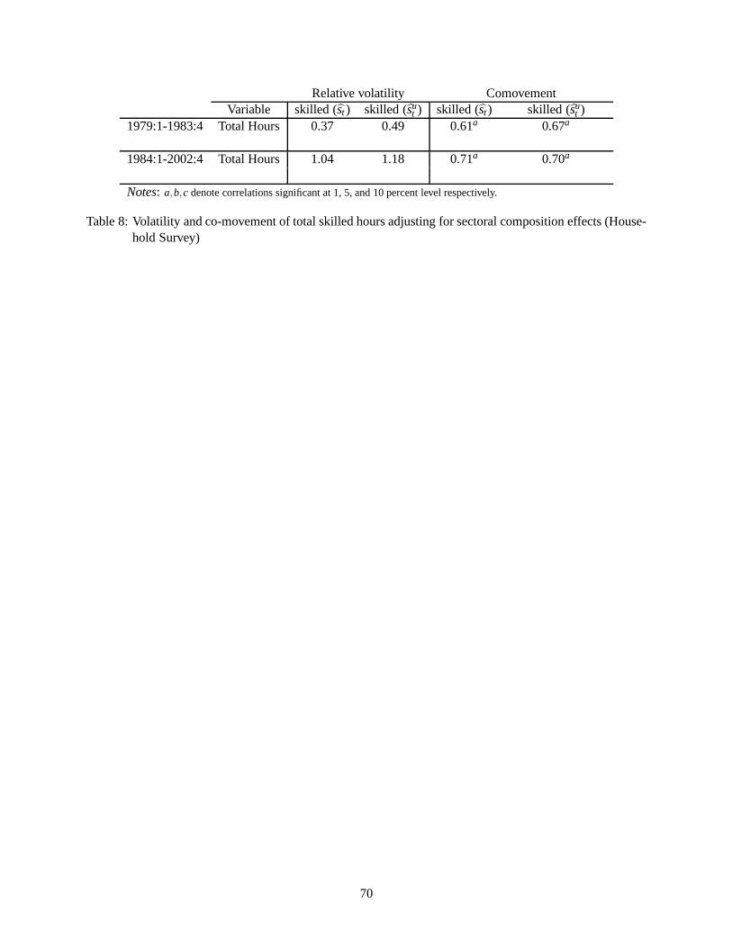
Relative volatility ComovementVariable skilled (st ) skilled (su

t ) skilled (st ) skilled (sut )

1979:1-1983:4 Total Hours 0.37 0.49 0.61a 0.67a

1984:1-2002:4 Total Hours 1.04 1.18 0.71a 0.70a

Notes: a,b,c denote correlations significant at 1, 5, and 10 percent levelrespectively.

Table 8: Volatility and co-movement of total skilled hours adjusting for sectoral composition effects (House-hold Survey)

70

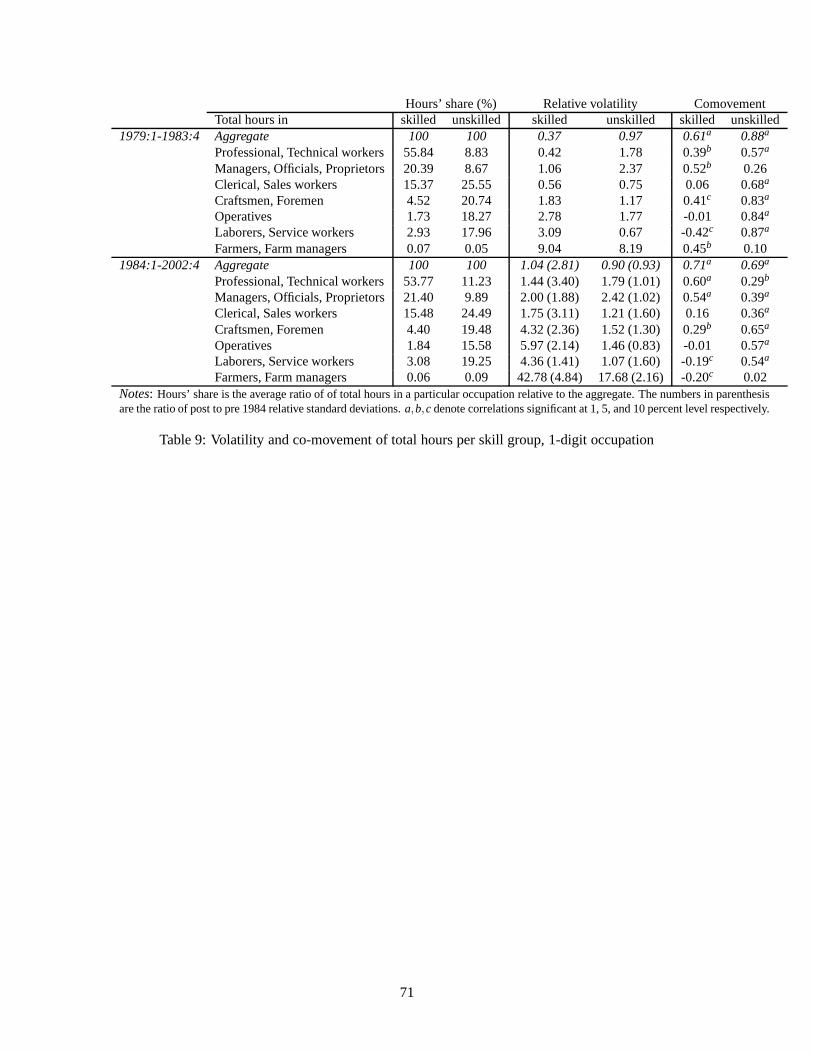
Hours’ share (%) Relative volatility ComovementTotal hours in skilled unskilled skilled unskilled skilled unskilled

1979:1-1983:4 Aggregate 100 100 0.37 0.97 0.61a 0.88a

Professional, Technical workers 55.84 8.83 0.42 1.78 0.39b 0.57a

Managers, Officials, Proprietors 20.39 8.67 1.06 2.37 0.52b 0.26Clerical, Sales workers 15.37 25.55 0.56 0.75 0.06 0.68a

Craftsmen, Foremen 4.52 20.74 1.83 1.17 0.41c 0.83a

Operatives 1.73 18.27 2.78 1.77 -0.01 0.84a

Laborers, Service workers 2.93 17.96 3.09 0.67 -0.42c 0.87a

Farmers, Farm managers 0.07 0.05 9.04 8.19 0.45b 0.101984:1-2002:4 Aggregate 100 100 1.04 (2.81) 0.90 (0.93) 0.71a 0.69a

Professional, Technical workers 53.77 11.23 1.44 (3.40) 1.79 (1.01) 0.60a 0.29b

Managers, Officials, Proprietors 21.40 9.89 2.00 (1.88) 2.42 (1.02) 0.54a 0.39a

Clerical, Sales workers 15.48 24.49 1.75 (3.11) 1.21 (1.60) 0.16 0.36a

Craftsmen, Foremen 4.40 19.48 4.32 (2.36) 1.52 (1.30) 0.29b 0.65a

Operatives 1.84 15.58 5.97 (2.14) 1.46 (0.83) -0.01 0.57a

Laborers, Service workers 3.08 19.25 4.36 (1.41) 1.07 (1.60) -0.19c 0.54a

Farmers, Farm managers 0.06 0.09 42.78 (4.84) 17.68 (2.16) -0.20c 0.02Notes: Hours’ share is the average ratio of of total hours in a particular occupation relative to the aggregate. The numbers in parenthesisare the ratio of post to pre 1984 relative standard deviations. a,b,c denote correlations significant at 1, 5, and 10 percent levelrespectively.

Table 9: Volatility and co-movement of total hours per skillgroup, 1-digit occupation

71

Relative volatility ComovementVariable skilled unskilled skilled unskilled

1979:1-1983:4 Total hours 0.45 1.00 0.38c 0.89a

Employment 0.49 0.81 0.01 0.87a

Average weekly hours of work 0.23 0.20 0.62a 0.83a

1984:1-2003:4 Total hours 1.56 0.89 0.56a 0.61a

Employment 1.34 0.77 0.48a 0.51a

Average weekly hours of work 0.37 0.37 0.47a 0.50a

Notes: a,b,c denote correlations significant at 1, 5, and 10 percent levelrespectively.

Table 10: Volatility and co-movement of total hours, employment and average weekly hours per skill group- Restricted sample: white, males, aged 31-55

72

Relative volatility ComovementVariable skilled unskilled aggregate skilled unskilled aggregate

1979:1-1983:4 Total hours 0.51 0.80 0.73 0.25 0.90a 0.91a

Employment 0.45 0.71 0.67 0.01 0.88a 0.87a

Average weekly hours of work 0.19 0.13 0.11 0.62a 0.82a 0.71a

1984:1-2003:4 Total hours 1.99 0.80 0.81 0.53a 0.75a 0.80a

Employment 1.85 0.74 0.73 0.50a 0.71a 0.76a

Average weekly hours of work 0.33 0.21 0.22 0.27b 0.44a 0.47a

Notes: a,b,c denote correlations significant at 1, 5, and 10 percent levelrespectively.

Table 11: Volatility and co-movement of total hours, employment and average weekly hours per skill group:alternative skill definition (skilled workers must have a master degree)

73

Relative volatility ComovementVariable skilled unskilled aggregate skilled unskilled aggregate

1976:1-1983:4 Employment 0.82 1.11 1.02 0.26 0.86a 0.87a

1984:1-2002:4 Employment 1.40 0.95 0.91 0.55a 0.77a 0.82a

Notes: a,b,c denote correlations significant at 1, 5, and 10 percent levelrespectively.

Table 12: Volatility and co-movement of total hours, employment and average weekly hours per skill group:Canadian Labour Force Survey

74