Why is the Snowflake Schema a Good Data Warehouse Design?

Mark Levene and George LoizouSchool of Computer Science and Information Systems

Birkbeck College, University of LondonMalet Street, London WC1E 7HX, U.K.

Email: {mark,george}@dcs.bbk.ac.uk

Abstract

Database design for data warehouses is based on the notion of the snowflake schemaand its important special case, the star schema. The snowflake schema represents adimensional model which is composed of a central fact table and a set of constituentdimension tables which can be further broken up into subdimension tables. We formalisethe concept of a snowflake schema in terms of an acyclic database schema whose join treesatisfies certain structural properties. We then define a normal form for snowflake schemaswhich captures its intuitive meaning with respect to a set of functional and inclusiondependencies. We show that snowflake schemas in this normal form are independentas well as separable when the relation schemas are pairwise incomparable. This impliesthat relations in the data warehouse can be updated independently of each other as longas referential integrity is maintained. In addition, we show that a data warehouse insnowflake normal form can be queried by joining the relation over the fact table with therelations over its dimension and subdimension tables. We also examine an information-theoretic interpretation of the snowflake schema and show that the redundancy of theprimary key of the fact table is zero.

Key words. Data warehouse design, star and snowflake schema, independent and separabledatabase schema, acyclic database schema.

1 Introduction

A data warehouse is an integrated and time-varying database primarily used for the supportof management decision making [Inm96, CD97, KRRT98]. A data warehouse often integratesheterogeneous data from multiple and distributed information sources and contains historicaland aggregated data. As an example, a sales data warehouse may contain information on theproducts sold, the time of sale, the place of sale and the sales person. Typically such a datawarehouse will be of orders of magnitude larger than an operational database which does notcontain specific sales data, but rather contains the company details, including details aboutproduct range, outlet locations and personnel.

In terms of data modelling it is beneficial to view a data warehouse in terms of a dimen-sional model which is composed of a central fact table and a set of surrounding dimensiontables each corresponding to one of the components or dimensions of the fact table. In theabove example the fact table models the actual sales data and each dimension, such as: the

1

product detail, the time of sale, the outlet in which the product was sold and the sales per-sonnel, is modelled by a separate dimension table. In relational database terms the facttable contains all the necessary foreign key attributes referencing the primary keys of theconstituent dimension tables. Conceptually this leads to a star-like data structure, which iscalled a star schema. According to [KRRT98] dimensional modelling actually predates theentity-relationship modelling approach, which is the conventional way in which to design arelational database coupled with normalisation theory [MR92, LL99]. Star schemas can berefined into snowflake schemas providing support for attribute hierarchies by allowing thedimension tables to have subdimension tables. For example, the dimension table storing theoutlet in which the product was sold may have a subdimension table containing demographicinformation of the area of sale. There is debate on the benefits of having such subdimensiontables, since it will, in general, slow down query processing, but in some cases it providesa necessary logical separation of data such as in the case of the demographic informationsubdimension [KRRT98].

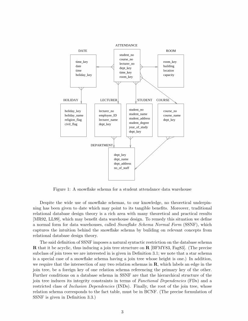
As a running example, we exhibit in Figure 1 a snowflake schema for a data warehouse forkeeping track of students’ attendance in a college. The fact table of this schema is ATTEN-DANCE, its dimension tables are DATE, ROOM, LECTURER, STUDENT and COURSEand finally HOLIDAY is a subdimension of DATE and DEPARTMENT is a subdimension ofLECTURER, STUDENT and COURSE. For clarity of the figure we have omitted the labelson edges, which for each edge between two tables is the intersection of their attributes. Thesnowflake schema is structured in such a way that the labels of edges represent a foreign toprimary key relationship between the parent table and its child. The meaning of the tables isself-evident from their attributes, observing that DEPARTMENT represents the departmentin which the course is given and not the department to which the student belongs. Thuslecturer no, student no and course no are only unique in the context of a particular depart-ment. (We note that we could derive a more complex schema by having additional foreignkeys in LECTURER and STUDENT pertaining to the respective departments to which theybelong.)

Although snowflake schemas enjoy a relatively simple structure they are widely used inpractice [KRRT98] and recommended in all the data warehouse design methodologies weare aware of to date. The reason for their success is that they are: intuitive and easy tounderstand, amenable to query optimisation since arbitrary n-way joins with the fact tablecan be evaluated by a single pass through the fact table, can accommodate for aggregate data,and are easily extensible by adding new attributes to the fact table or to one or more of thedimension tables and new dimension tables to the schema without interfering with existingdatabase programs.

There has been some recent research on formalising data warehouses using a graph-theoretic approach to model snowflake schemas. In [GMR98] it is shown how a snowflakeschema can be derived from an entity-relationship diagram and then modified accordinglyto remove uninteresting attributes. In [LAW98] several normal forms were defined for datawarehouses within a general multidimensional model where functional dependencies induceattribute hierarchies. More recently, a methodology for deriving a snowflake schema from anoperational database schema has been presented in [HLV00]. Finally, it is worth mentioning[KM00] where the concept of a data webhouse is introduced. A data webhouse is essentiallya data warehouse intended to capture clickstream log data for ecommerce decision making.

2

holiday_key holiday_namereligion_flagcivil_flag

time_keydatetimeholiday_key

room_key buildinglocationcapacity

dept_keydept_namedept_addressno_of_staff

student_no student_namestudent_addressstudent_degreeyear_of_study dept_key

course_no course_namedept_key

lecturer_no employee_IDlecturer_namedept_key

student_no course_no lecturer_no dept_key time_key room_key

DATE

ATTENDANCE

ROOM

HOLIDAY LECTURER STUDENT COURSE

DEPARTMENT

Figure 1: A snowflake schema for a student attendance data warehouse

Despite the wide use of snowflake schemas, to our knowledge, no theoretical underpin-ning has been given to date which may point to its tangible benefits. Moreover, traditionalrelational database design theory is a rich area with many theoretical and practical results[MR92, LL99], which may benefit data warehouse design. To remedy this situation we definea normal form for data warehouses, called Snowflake Schema Normal Form (SSNF), whichcaptures the intuition behind the snowflake schema by building on relevant concepts fromrelational database design theory.

The said definition of SSNF imposes a natural syntactic restriction on the database schemaR that it be acyclic, thus inducing a join tree structure on R [BFMY83, Fag83]. (The precisesubclass of join trees we are interested in is given in Definition 3.1; we note that a star schemais a special case of a snowflake schema having a join tree whose height is one.) In addition,we require that the intersection of any two relation schemas in R, which labels an edge in thejoin tree, be a foreign key of one relation schema referencing the primary key of the other.Further conditions on a database schema in SSNF are that the hierarchical structure of thejoin tree induces its integrity constraints in terms of Functional Dependencies (FDs) and arestricted class of Inclusion Dependencies (INDs). Finally, the root of the join tree, whoserelation schema corresponds to the fact table, must be in BCNF. (The precise formulation ofSSNF is given in Definition 3.3.)

3

Our definition of SSNF captures the intuition behind data warehouse design and ourresults provide semantic justification for the definition of SSNF. To motivate these resultswe briefly describe the concepts of independent [Sag83, AC91, Sag91] and separable [CM87]database schemas R with respect to a set of integrity constraints Σ consisting of FDs and INDsover R. Given a database d over R, independence implies that maintaining local consistencyof the relations in d, i.e. ensuring that d satisfies the INDs in Σ and that the relationsin d satisfy the FDs in Σ, is sufficient to ensure global consistency, i.e. the existence of arepresentative instance over the set of all attributes U in R that satisfies the set F of FDs(see Definition 2.14). The reason the representative instance is an important concept is thatit provides us with a means of testing the satisfaction of interrelational constraints, whichmay hold in the join of several relations in d. Separability is an extension of independence,which, in addition, implies that updates to relations in d are independent in the sense thatwe cannot deduce additional tuples in any relation in d via a join of several relations in thedatabase d. We show that when R is in SSNF with respect to Σ then it is independent, andif, in addition, the relation schemas in R are incomparable then it is also separable. Thus fordatabase schemas in SSNF integrity maintenance in the presence of updates is easily enforced.We also show that tuples in the representative instance over U , i.e. tuples over the fact tableextended with the relevant information in the constituent dimension tables, can be computedvia the snowflake join (cf. star join [OG95]). This implies that the results of queries over adata warehouse which is in SSNF maintain their consistency, i.e. satisfy the induced set ofFDs over their schema.

We also examine an information-theoretic interpretation of the snowflake schema followingthe work of [Mal86, CP87, Lee87, Mal88], which allows us to accommodate probabilisticinformation in the data warehouse. This is especially important, since decision making ofteninvolves probabilistic reasoning [Lin85]. We show that the redundancy in the snowflake join ofthe primary key of the fact table is zero, i.e. it is minimal. Against this measure of redundancy,which is the standard evaluation criterion for assessing relational database schemas, SSNF isoptimal.

In summary the paper establishes a theoretical underpinning for data warehouse design bybuilding upon an acyclic structure and utilising the notions of independence and separability.Since, to our knowledge, there is no formal definition of the concept of a snowflake schemato be found in the data warehousing literature it is not possible to give a formal proof of theequivalence of SSNF and the intuitive concept of a snowflake schema. The best we can offer isa “concept of proof” in the sense that all examples of snowflake schemas we have encounteredin the literature satisfy SSNF.

The layout of the rest of the paper is as follows. In Section 2 we present the backgroundin relational database theory necessary for the rest of the paper. In Section 3 we formalise thenotion of a snowflake schema, define SSNF and present our results concerning the beneficialproperties of snowflake schemas. In Section 4 we analyse the snowflake schema from aninformation-theoretic point of view and show that its entropy has a particularly simple form.Finally, in Section 5 we give our concluding remarks.

4

2 Relations and Data Dependencies

We now present the background material necessary for the development of the ideas in thepaper; see [LL99] for additional details on relational database theory.

We use the notation |S| to denote the cardinality of a set S. If S is a subset of T we write S⊆ T and if S is a proper subset of T we write S ⊂ T. Furthermore, S and T are incomparableif S 6⊆ T and T 6⊆ S. We often denote the singleton {A} simply by A, and the union of twosets S, T, i.e. S ∪ T, simply by ST.

Definition 2.1 (Database schema and database) Let U be a finite set of attributes. Arelation schema R is a finite sequence of distinct attributes from U .

A database schema over U is a finite set R = {R0, R1, . . . , Rn}, such that each Ri ∈ R isa relation schema and

⋃i Ri = U .

We assume a countably infinite domain of values, D, partially ordered; without loss ofgenerality we assume that D is an antichain, i.e. ∀c1, c2 ∈ D, c1 ≤ c2 if and only if c1 = c2.The domain of R, denoted as DOM(R), is defined as the Cartesian product D × . . .×D (|R|times). An R-tuple (or simply a tuple whenever R is understood from context) is a memberof DOM(R).

A relation r over R is a finite (possibly empty) set of R-tuples. A database d over R is afamily of n + 1 relations {r0, r1, . . . , rn} such that each ri ∈ d is over Ri ∈ R.

From now on we let R = {R0, R1, . . . , Rn} be a database schema over U and d ={r0, r1, . . . , rn} be a database over R. Furthermore, we let r ∈ d be a relation over a re-lation schema R ∈ R. As usual uppercase letters (which may be subscripted) from the end ofthe alphabet such as X, Y, Z will be used to denote sets of attributes, while those from thebeginning of the alphabet such as A, B, C will be used to denote single attributes or singletonsets of attributes.

Definition 2.2 (Projection) The projection of an R-tuple t onto a set of attributes Y ⊆R, denoted by t[Y], is the restriction of t to Y. The projection of a relation r over R onto Y⊆ R, denoted as πY(r), is defined by πY(r) = {t[Y] | t ∈ r}. The projection of a relation sover U onto R, denoted as πR(s), is the database {πR0(s), πR1(s), . . . , πRn(s)}.

Definition 2.3 (Natural join) The natural join (or simply the join), 1, of two relations r1

over R1 and r2 over R2 is a relation r over R = R1 ∪R2 defined by

r1 1 r2 = {t | ∃t1 ∈ r1 and ∃t2 ∈ r2 such that t[R1] = t1 and t[R2] = t2}.

Definition 2.4 (Join dependency) A Join Dependency (or simply a JD) for a databaseschema R is a statement of the form 1[R]. A JD 1[R] is said to be trivial if one of itscomponents is U .

A JD 1[R] is satisfied in a relation r over U , (alternatively, R is a lossless join decompo-sition of U), denoted by r |= 1[R], if

r = πR0(r) 1 πR1(r) 1 . . . 1 πRn(r).

5

Definition 2.5 (Functional dependency) A Functional Dependency over U (or simply anFD) is a statement of the form X → Y, where X, Y ⊆ U are sets of attributes. An FD of theform X → Y is said to be trivial if Y ⊆ X.

An FD X → Y is satisfied in a relation r ∈ d over R, denoted by r |= X → Y, wheneverXY ⊆ R and ∀t1, t2 ∈ r, if t1[X] = t2[X] then t1[Y] = t2[Y]. A relation r ∈ d satisfies a set Fof FDs over U , if for all α ∈ F, r |= α.

From now on we let F be a set of FDs over U .

Definition 2.6 (Closure) The set of FDs that are logically implied by F is denoted by F+.A set of FDs G over U is a cover of F if G+ = F+.

The closure of a set of attributes X ⊆ U with respect to F, denoted by CF(X), is the setof attributes {A | X → A ∈ F+}.

Definition 2.7 (Embedded FDs and dependency preservation) The projection of Fonto a relation schema R, denoted by F+|R, is the set of FDs X → Y ∈ F+ such that XY ⊆R. An FD X → Y is embedded in R if XY ⊆ R.

A database schema R is dependency preserving with respect to F (alternatively R preservesF) if there is a cover G of F such that each FD X → Y ∈ G is embedded in some Ri ∈ R.

From now on we assume that R is a dependency preserving database schema with respectto F and let Fi be a cover of F+|Ri which is embedded in Ri; we assume without loss ofgenerality that Fi is a canonical cover, i.e. for all X → Y ∈ Fi, Y = {A} is a singleton andA 6∈ X. (See [LL99] for more details on the formal properties of FDs.)

Definition 2.8 (Inclusion dependency) An Inclusion Dependency (or simply an IND)over R is a statement of the form Ri[X] ⊆ Rj [Y], where Ri, Rj ∈ R and X ⊆ Ri, Y ⊆ Rj aresequences of distinct attributes such that |X| = |Y|. An IND is said to be trivial if it is of theform R[X] ⊆ R[X]. An IND is said to be typed if it is of the form R[X] ⊆ S[X].

An IND Ri[X] ⊆ Rj [Y] over R is satisfied in d, denoted by d |= Ri[X] ⊆ Rj [Y], wheneverπX(ri) ⊆ πY(rj), where ri, rj ∈ d are the relations over Ri and Rj , respectively. A databased over R satisfies a set I of INDs over R, if for all α ∈ I, d |= α.

From now on we let I be a set of INDs over R and let Σ = F ∪ I. A database d over Rsatisfies Σ, denoted by d |= Σ, whenever each ri ∈ d satisfies all the FDs in Fi and d satisfiesall the INDs in I. Also, we denote by Σ+ the set of FDs and INDs that are logically impliedby Σ.

Definition 2.9 (Graph representation of INDs) The graph representation of a set ofINDs I over R is a directed graph GI = (N, E), which is constructed as follows. Each relationschema R in R has a separate node in N labelled by R, i.e. we do not distinguish betweennodes and their labels. There is an edge (R, S) ∈ E if and only if there is a nontrivial INDR[X] ⊆ S[Y] ∈ I.

Definition 2.10 (Dag-like INDs) A set I of INDs over R is dag-like if

6

1) I is a set of typed INDs, and

2) GI is a rooted directed acyclic graph.

Definition 2.11 (Keys and key-based INDs) A set of attributes X ⊆ Ri is a superkeyfor Ri with respect to Fi (or simply X is a superkey for Ri if Fi is understood from context) ifCFi(X) = Ri holds; X is a key for Ri with respect to Fi if it is a superkey for Ri with respectto Fi and for no proper subset Y ⊂ X is Y a superkey for Ri with respect to Fi. The primarykey of Ri is one of the keys for Ri with respect to Fi, which is designated by the databasedesigner.

A database schema R is in Boyce-Codd Normal Form (or simply BCNF) with respect toF if for all Ri ∈ R, for all nontrivial FDs X → Y ∈ Fi, X is a superkey for Ri with respect toFi.

An IND Ri[X] ⊆ Rj [Y] is superkey-based (key-based) if Y is a superkey (key) for Rj withrespect to Fj . When Y is the primary key of Rj then X is called a foreign key of Ri.

Definition 2.12 (No interaction between FDs and INDs) A set Σ = F ∪ I of FDs andINDs do not interact when X → Y ∈ Σ+ if and only if X → Y ∈ F+ and R[X] ⊆ S[Y] ∈ Σ+

if and only if R[X] ⊆ S[Y] ∈ I+.

In Section 3 we will show that for the subclass of dag-like INDs we are interested in, Fand I do not interact.

The chase procedure provides us with a very useful algorithm which forces a database tosatisfy a set of integrity constraints.

Definition 2.13 (Chase procedure for FDs) We assume a countably infinite domain ofmarked nulls, V, which is disjoint from D; without loss of generality we assume that V islinearly ordered and that ∀c ∈ D, ∀v ∈ V, c < v.

Given a tuple t ∈ ri, where ri ∈ d is over Ri ∈ R, pad(t) is a tuple over U such thatpad(t)[Ri] = t, and for all A ∈ U −Ri, pad(t)[A] ∈ V, i.e. it is a marked null. Given a relationri ∈ d over Ri ∈ R we define pad(ri) =

⋃t∈ri

pad(t), and pad(d) =⋃

ri∈d pad(ri), such thatfor all t1, t2 ∈ pad(d), for all A, B ∈ U , if t1[A], t2[B] ∈ V, and either t1 6= t2 or A 6= B, thent1[A] 6= t2[B], i.e. all marked nulls in distinct positions of pad(d) are distinct.

The chase of d with respect to a set F of FDs over U , denoted by CHASE(d, F), is theresult of applying the FD rule, as defined below, to the current state, say r, of CHASE(d,F) until it cannot be further applied to r or until a contradiction is detected. The state ofCHASE(d, F) prior to the first application of the FD rule is pad(d).

FD rule: If X → Y ∈ F and ∃t1, t2 ∈ r such that t1[X] = t2[X] but t1[Y] 6= t2[Y], then

1) if for some A ∈ Y such that t1[A] 6= t2[A] and t1[A], t2[A] ∈ D, then a contradictionis detected, otherwise

2) for all A ∈ Y, change all the occurrences in r of the larger of the values of t1[A]and t2[A] to the smaller of the values of t1[A] and t2[A].

7

Often we refer to an application of the FD rule during the computation of the chase as achase step. When the FD rule cannot be further applied to the current state, r, of CHASE(d,F) or a contradiction is detected, then we remove subsumed tuples from the result to obtainCHASE(d, F). A tuple t2 is subsumed by a tuple t1, if t1 6= t2 and for all A ∈ U , t1[A] ≤t2[A].

We note that all operations that we have defined on relations, including dependencysatisfaction, equally apply to relations which have marked nulls in them. We further notethat, on treating the marked nulls in CHASE(d, F) as distinct domain values, CHASE(d, F)|= F if and only if no contradictions are detected during the computation of the chase [Hon82].

Definition 2.14 (Representative instance and consistency) The representative instance[Sag83] of d with respect to F, denoted as RIF(d) (or simply RI(d) whenever F is understoodfrom context), is constructed as follows. First we invoke the chase procedure on pad(d) withrespect to F. If CHASE(d, F) |= F, then we set RI(d) to CHASE(d, F), otherwise we setRI(d) to pad(d). In either case we replace all the marked nulls in the resulting relation withthe minimum value of all these marked nulls.

If there are no contradictions in CHASE(d, F) then we say that RI(d) satisfies F, denotedby RI(d) |= F. A database d is said to be consistent with respect to F if RI(d) |= F, otherwiseit is said to be inconsistent with respect to F.

Definition 2.15 (Independent and separable database schemas) A database schemaR is said to be independent [Sag83, AC91, Sag91] with respect to Σ if for all databases d overR, d |= Σ implies that RI(d) |= F, i.e. d satisfies Σ implies that d is consistent with respectto F.

For a relation s over U , which may contain marked nulls, we define π↓R(s) to be thedatabase obtained from πR(s) after removing from each resulting relation over Ri all tuplesthat have at least one marked null over any attribute in Ri.

A database schema R is said to be separable [CM87] with respect to Σ if R is independentwith respect to Σ and for all d over R such that d |= Σ, d = π↓RRI(d).

We next define the notion of an acyclic database schema [Fag83] by using the concept ofa join tree [BFMY83].

Definition 2.16 (Join tree and acyclic database schema) A join tree for R is a treewhose node set is R such that

1) each of its edges (R, S) is labelled by the nonempty set of attributes R ∩ S; and

2) for every distinct pair R, S ∈ R and for every attribute A ∈ R ∩ S, each edge along theunique path between R and S includes A in its label.

A database schema R is acyclic if it has a join tree, which we denote by JT(R).

8

Definition 2.17 (Rooted tree) When we distinguish a node in a tree, T, as its root, wecan view T as a directed graph with unique directed paths from the root of T to all its leaves[BH90].

From now on we will assume that trees are rooted and consider them as special cases ofdirected acyclic graphs.

We define the height of a node n in a tree T recursively as follows: if n is the root node ofT then its height is zero, otherwise the height of n is one plus the height of its parent node.The height of T is defined to be the maximal height among all the leaf nodes of T.

A topological sort of a directed acyclic graph G is a process of assigning a linear orderingto the nodes of G so that if there is an edge in G from node ni to node nj , then ni precedesnj in the linear ordering.

We say that a node nj is a descendant of a node ni in G if there is a directed path fromni to nj ; we take ni to be a descendant of itself. (We take parent to be irreflexive.)

3 The Snowflake and Star Schemas

We formalise the notion of a snowflake schema and its important special case the star schemaas an acyclic database schema having a join tree which satisfies two structural properties. Wethen define a normal form for snowflake schemas with respect to a set of FDs and INDs andshow that it has several fundamental desirable properties. In particular, our results implythat the relations over the fact and dimension tables can be updated independently of eachother as long as referential integrity is maintained. Moreover, we show that when in SSNFthe data warehouse can be queried via the snowflake join which is the join of the relation overthe fact table with the relations over its dimension and subdimension tables.

We next present the notion of a snowflake schema as a special kind of an acyclic databaseschema.

Definition 3.1 (Snowflake and star schema) A database schema R is a snowflake schemaif it is acyclic and its join tree has a designated root, which we take to be R0, satisfying thefollowing structural conditions:

1) no two distinct edges have identical labels; and

2) if there is a label Xj in JT(R) such that {Xi1, Xi2, . . . , Xim} is the set of all labels inJT(R), satisfying Xj ⊂ Xik, for k = 1, 2, . . . , m, and for no Xik in this set does thereexist a label X ′ in JT(R) satisfying Xj ⊂ X ′ ⊂ Xik, then for some k ∈ {1, 2, . . . , m},Rik is the parent node of Rj in JT(R), where Xj = Rik ∩Rj and Xik = Ri ∩Rik is thelabel of the edge (Ri, Rik), Ri being the parent of Rik in JT(R).

If R is a snowflake schema and the height of JT(R) is one, then R is called a star schema.When R is a snowflake schema, R0 is called the fact table while the Ri’s of height one are

called the dimension tables and the remaining relation schemas of height greater than one arecalled the subdimension tables.

9

We observe that condition (1) above is a restriction on the class of acyclic databaseschemas while condition (2), which does not restrict the class of acyclic database schemas,restricts the class of join trees. The motivation for condition (1) stems from the fact thatlabels of the form Xi represent primary keys and thus there is no justification for having twoseparate relation schemas having identical primary keys, since they can be coalesced into asingle relation schema. Regarding condition (2) it enforces a hierarchical dependence of theprimary keys of relation schemas in terms of their set inclusion relationship, thereby modellingmany-to-one relationships.

Referring back to the running example of Figure 1, suppose we remove any two of theincoming edges to DEPARTMENT; for concreteness assume we remove the edges from LEC-TURER to DEPARTMENT and from STUDENT to DEPARTMENT. Then it can be seenthat conditions (1) and (2) are satisfied for this schema and thus it is a snowflake schema.Regarding condition (1) the labels on the two edges from ATTENDANCE to LECTURERand STUDENT represent the primary keys of the two latter dimension tables, and regardingcondition (2) {dept key} is the largest proper subset of {course no, dept key} that is also thelabel of the edge from COURSE to DEPARTMENT.

The next definition of the join graph of a snowflake schema ensures that such hierarchicaldependence is maintained between all its dimensions and subdimensions.

Definition 3.2 (The join graph of a snowflake schema) We convert the join tree, JT(R),of a snowflake schema R, into a directed acyclic graph, called the join graph of R and de-noted by JG(R), as follows. For every relation schema Ri, whose parent is R′

i and such thatXi = R′

i ∩Ri, add an edge from Ri to Rj whose parent is R′j with Xj = R′

j ∩Rj , if Xj ⊂ Xi

and there is no other label X ′ in JT(R) satisfying Xj ⊂ X ′ ⊂ Xi. The label of the new edge(Ri, Rj) is Xj .

We note that in JG(R) if a node has more than one parent, then the labels of its incomingedges are identical; this is a byproduct of R being acyclic. We further note that JG(R) isacyclic, since the new edges are oriented away from the root node.

Referring back to Figure 1, consider the join tree resulting from removing the edges fromLECTURER and STUDENT to DEPARTMENT. The resulting join tree satisfies Defini-tion 3.1. On using Definition 3.2 we convert the said join tree to the corresponding join graphby adding the edges from LECTURER and STUDENT to DEPARTMENT.

Let R be a snowflake schema. From now on we assume that whenever Ri and Rj aredistinct relation schemas in R, then i < j if and only if Ri precedes Rj in a topological sortof JG(R). Moreover, we let

1) Xi = Rj ∩Ri, for i = 1, . . . , n, where Rj is the parent node of Ri in JT(R), be the labelof the edge from Rj to Ri;

2) X0 =⋃k

i=1 Xi, where {R1, R2, . . . , Rk} is the set of children of R0 in JT(R); and

3) Yi = Ri −Xi, for i = 0, 1, . . . , n.

We observe that for all i, j ∈ {0, 1, . . . , n}, with i 6= j, Yi ∩ Yj = ∅.We next define a normal form for snowflake schemas which imposes further restrictions

on the labels of edges in the join tree of R taking into account the functional and inclusion

10

dependencies. The main motivation behind the definition is that it encapsulates the intu-itions behind the snowflake schema, which have been advocated by database practitioners,by capturing the hierarchical dependence between dimensions and subdimensions via the jointree and data dependency information via primary key to foreign key relationships.

Definition 3.3 (Snowflake schema normal form) A database schema R is in SnowflakeSchema Normal Form (SSNF) with respect to a set Σ = F ∪ I of FDs and INDs over R (orsimply in SSNF if Σ is understood from context), if

1) R is a snowflake schema;

2) R0 is in BCNF with respect to F0;

3) for i = 0, 1, . . . , n, Xi is the primary key of Ri with respect to Fi;

4) for i = 0, 1, . . . , n, CF(Ri) =⋃

j≥i Rj such that Rj is a descendant of Ri in JG(R); and

5) I = {Ri[Xj ] ⊆ Rj [Xj ] | i, j ∈ {0, 1, . . . , n} and Ri is a parent of Rj in JG(R)} is a setof INDs over R.

Condition (1) is a structural restriction that was motivated after Definition 3.1. Condi-tion (2) minimises the redundancy of the relation over the fact table. Condition (3) is thestandard requirement of a snowflake schema [KRRT98]. It implies that R is a lossless joindecomposition of U [LL99]. Condition (4) maximises the efficiency of queries involving rela-tions over dimension/subdimension tables, since it specifies that the sequence of joins thatis needed to query information emanating from any such table involves only itself and itssubdimension tables. Condition (5) guarantees referential integrity, noting that I is dag-likeby (1) and key-based by (3). We observe that due to (1) and (3) it is always true that

⋃j≥i

Rj ⊆ CF(Ri).

The following lemma is a corollary of the main result in [LL01] due to the special structureof snowflake schemas.

Lemma 3.1 If Σ is in SSNF then F and I do not interact. 2

We note that as a result of Lemma 3.1 we obtain the desirable property that the implicationproblem for FDs or INDs in Σ is polynomial-time decidable [BB79, CV83]. (In general, whenthere is interaction between the FDs and INDs, the implication problem for FDs and typedINDs, with acyclic GI , is NP-hard [CK86].)

The next lemma shows that in the special case when only primary and foreign keys arespecified then R is in SSNF. This special case of SSNF is important, since it is directly inducedby the structure of a snowflake schema and reflects practitioners’ intuition.

Lemma 3.2 Let R be a snowflake schema and F = {X0 → Y0, X1 → Y1, . . . , Xn → Yn} bea set of FDs over U , where for i = 1, 2, . . . , n, F+|Xi contains only trivial FDs. Also, let I ={Ri[Xj ] ⊆ Rj [Xj ] | i, j ∈ {0, 1, . . . , n} and Ri is a parent of Rj in JG(R)} be a set of INDsover R. Then R is in SSNF with respect to Σ, where Σ = F ∪ I.

11

Proof. Conditions (1) and (5) of SSNF are evident from the statement of the lemma, so itremains to show that conditions (2), (3) and (4) hold.

To prove (2) it is sufficient to show that {X0 → Y0} is a cover of F0. By Definition 3.1and the notation introduced after Definition 3.2 we have that for all Ri distinct from R0 wehave Yi∩R0 = ∅. Moreover, Y0∩Xi = ∅, so the result follows. (In fact, with the assumptionsof the lemma it is not hard to show the tighter result that R is in BCNF with respect to F.)

Condition (3) follows from the assumption that, for i = 1, 2, . . . , n, F+|Xi contains onlytrivial FDs and the fact that R0 is in BCNF with respect to F0.

It remains to establish (4). By the observation after Definition 3.3 we have⋃

j≥i Rj ⊆CF(Ri), so we need to show that CF(Ri) ⊆

⋃j≥i Rj . Suppose that this is not the case. Then,

for some relation schema Rj which is not a descendant of Ri we have a nontrivial FD Xj

→ A ∈ F+, where Xj ⊆ CF(Ri) and A 6∈ Ri. By the structure of F and Definition 2.16 itfollows that Xj ⊆ Xi. By part (1) of Definition 3.1 Xj 6= Xi implying that Xj ⊂ Xi, and byof Definitions 3.1 and 3.2 Rj must be a descendant of Ri. This concludes the result. 2

Referring back to Figure 1 let R be the snowflake schema comprising the tables inthe figure and let F and I be the set of FDs and INDs over R, which are induced bythe structure of its join tree. That is, F = {time key → {date, time, holiday key}, holi-day key →{holiday name, religion flag, civil flag}, {lecturer no, dept key} → {employee ID,lecturer name}, {student no, dept key} → {student name, student address, student degree,year of study}, {course no, dept key} → course name, room key → {building, location, ca-pacity}, dept key→{dept name, dept address, no of staff}} and I = {ATTENDANCE[time key]⊆DATE[time key], DATE[holiday key]⊆HOLIDAY[holiday key], ATTENDANCE[lecturer no,dept key]⊆ LECTURER[lecturer no, dept key], LECTURER[dept key]⊆DEPARTMENT[dept key],ATTENDANCE[student no, dept key]⊆ STUDENT[student no, dept key], STUDENT[dept key]⊆ DEPARTMENT[dept key], ATTENDANCE[course no, dept key] ⊆ COURSE[course no,dept key], COURSE[dept key] ⊆ DEPARTMENT[dept key], ATTENDANCE[room key] ⊆ROOM[room key]}. It follows by Lemma 3.2 that R is in SSNF with respect to Σ = F ∪ I.

The next result shows that SSNF implies independence, and if, in addition, the relationschemas in R are pairwise incomparable then SSNF implies separability.

Theorem 3.3 The following statements are true:

1) If R is in SSNF with respect to Σ then it is independent with respect to Σ.

2) If R is in SSNF with respect to Σ and for all i, j ∈ {0, 1, . . . , n}, with i 6= j, Ri and Rj

are incomparable, then it is separable with respect to Σ.

Proof. Let t ∈ pad(d) originate from Ri and let t′ ∈ r′, where r′ is the current state ofCHASE(d, F) and t′ is the current state of t. Moreover let ρ(t′) be the set of all attributesA ∈ U such that either t′[A] is nonnull or is a marked null which was equated to someother marked null in obtaining r′ from pad(d). Thus ρ(t) = Ri and ρ(t) ⊆ ρ(t′). Moreover,ρ(t′) ⊆ CF(Ri) by a straightforward induction on the number of chase steps which wereapplied to pad(d) in order to obtain r′.

For part (1) we assume that R is in SSNF with respect to Σ but is not independent withrespect to Σ. Thus there is a database d over R such that d |= Σ but RI(d) is inconsistentwith respect to F. Consider the first chase step, during the computation of CHASE(d, F),

12

which detects a contradiction when applying an FD, say X → A, to the two tuples, say t′i andt′j , in the current state of the chase. Moreover assume that t′i and t′j , are the current states ofti, tj ∈ pad(d) originating from Ri and Rj , respectively. It follows that XA ⊆ CF(Ri), CF(Rj).

We claim that i and j are such that either Ri is a descendant of Rj in JG(R) or viceversa. To prove the claim assume that neither Ri nor Rj is a descendant of the other inJG(R). Now, by condition (4) of SSNF XA is a subset of the union of the descendant relationschemas of both Ri and Rj . Therefore, by condition (1) of SSNF, it must be the case thatXA ⊆ Ri, Rj , since R being acyclic implies that each edge along the unique path in JT(R)between Ri and Rj includes XA in its label. However, XA cannot be a subset of any key forany relation schema with respect to its set of FDs; this contradicts condition (3) of SSNF.Hence the said claim follows.

There are two further steps to consider. Firstly, consider the case when i = j. Let Ybe the maximal set of attributes Y ⊆ Ri such that Y ⊆ X and XA ⊆ CF(Y). Now, if A∈ Ri then, since both t′i and t′m are the current states of two distinct tuples, say ti andtm, which originate from Ri, it must be that t′i[YA] = ti[YA] and t′m[YA] = tm[YA]. Thusri 6|= X → A, which contradicts our assumption that d |= F implying that RI(d) must beconsistent. On the other hand, if A 6∈ Ri, then due to condition (4) of SSNF A ∈ Rik

for some descendant Rik of Ri. Thus by condition (5) of SSNF we have a chain of INDs,Ri[Xi1] ⊆ Ri1[Xi1], Ri1[Xi2] ⊆ Ri2[Xi2], . . . , Ri(k−1)[Xik] ⊆ Rik[Xik] such that by condition(3) of SSNF Xij is the primary key of Rij , for j = 1, 2, . . . , k, and Xi1 ⊆ Y. It follows thatrik 6|= Xik → A, which contradicts our assumption that d |= F implying that RI(d) must beconsistent. We note that A cannot be a member of two relation schemas on distinct pathsleading out of Ri, since by the acyclicity of R this would imply that A ∈ Ri.

Secondly, consider the case when i 6= j; assume without loss of generality that Rj is adescendant of Ri. We consider the various possibilities for A to be included in Ri or Rj . If A∈ Ri, then it is also the case that A ∈ Rj , since XA ⊆ CF(Ri), CF(Rj), and thus XA ∈ Ri∩Rj

contradicting the fact that Xj is a key for Rj . If A ∈ Rj but A 6∈ Ri, then we can deducethat rj 6|= X ′ → A, for some subset X ′ ⊆ Xj , which contradicts our assumption that d |= Fimplying that RI(d) must be consistent. Finally, if A 6∈ Ri, Rj , then by an argument similarto the case when i = j we can arrive at a contradiction of our assumption that d |= F, whichimplies that RI(d) must be consistent.

For part (2) we need to show that for all d over R such that d |= Σ, d = π↓RRI(d). Let dbe a database over R and assume that d |= Σ. By part (1) d is consistent, i.e. RI(d) |= F.Let d′ = π↓RRI(d).

Let r′i be the relation in d′ over Ri ∈ R. We need to show that r′i = ri, where ri is therelation in d over Ri. Let tj ∈ pad(d) originate from Rj , with j 6= i, and let t′j ∈ RI(d) be thefinal state of tj . Assume that t′j [Ri] is nonnull and thus CF(Ri) ⊆ CF(Rj). We claim thatt′j [Ri] ∈ ri proving the result.

There are three cases to consider. In the first case neither Ri nor Rj is a descendant of theother in JG(R). It follows that Ri ⊆ Rj by conditions (1) and (4) of SSNF, since R is acyclic,which contradicts our assumption that Ri and Rj are incomparable. In the second case Ri

is a descendant of Rj in JG(R). By condition (5) of SSNF tj [Xi] = ti[Xi] for some ti ∈ ri,and by condition (3) of SSNF and the fact that d is consistent it follows that t′j [Ri] = ti asrequired. In the third case Rj is a descendant of Ri in JG(R). By condition (4) of SSNF wehave CF(Ri) = CF(Rj). Moreover, by the incomparability of Ri and Rj there is an attribute,

13

say A, in Ri−Rj that does not appear in the label of any edge in JG(R) on the unique pathbetween Ri and Rj . Thus by condition (4) of SSNF A 6∈ CF(Rj) leading to a contradiction.This proves the result. 2

In part (2) of Theorem 3.3 we cannot relax the restriction that the Ri in R be incompa-rable. As a counterexample consider a database schema R = {R0, R1}, with R0 ⊂ R1. Inthis case R is not separable with respect to Σ = {R0[R0] ⊆ R1[R0], R0 → (R1 −R0)}, since,in general, r0 ⊂ πR0(r1), where d = {r0, r1} is a database over R satisfying Σ.

We next define the snowflake join of a database d over a snowflake schema R.

Definition 3.4 (Snowflake join and star join) Let R be a snowflake schema and let Rα0 ,Rα1 , . . ., Rαn be a topological sort of JG(R). The snowflake join of a database d over R,denoted as SNOW(d), is given by

SNOW(d) = (· · · (rα0 1 rα1) 1 · · · 1 rαn).

When R is a star schema then SNOW(d) is called the star join of d.

The next theorem shows that the snowflake join contains the tuples over the fact tableextended with the relevant information in the constituent dimension and subdimension tables.This implies that the results of queries over a data warehouse, which is in SSNF, maintaintheir consistency, i.e. satisfy the projected set of FDs over their schema.

Theorem 3.4 Let R be in SSNF with respect to Σ. Then RI↓(d) = SNOW(d), if d |= Σ,where RI↓(d) is the set of all tuples in RI(d) having no null values in them.

Proof. Suppose that d |= Σ and thus by Theorem 3.3 d is consistent, i.e. RI(d) = CHASE(d,F) and RI(d) |= F. We prove the result by induction on the height, say k, of JT(R).

(Basis): If k = 0, then the result is trivial, since d = {r0} and thus RI(d) = RI↓(d) = r0,since by hypothesis d |= Σ.

(Induction): Assume the result holds when the height of JT(R) is k, with k ≥ 0; we thenneed to prove that the result holds when the height of JT(R) is k + 1.

Let Rα0 , Rα1 , . . . , Rαm be the set of all relation schemas in JT(R) whose height is lessthan or equal to k, and let dk = {rα0 , rα1 , . . . , rαm}. Then by inductive hypothesis, notingcondition (2) of Definition 3.1, we have

RI↓(dk) = SNOW(dk) = (· · · (rα0 1 rα1) 1 · · · 1 rαm).

Now, let Rαm+1 , . . . , Rαn be the remaining relation schemas in R whose height in JT(R)is k + 1. It remains to show that

RI↓(d) = (· · · (RI↓(dk) 1 rαm+1) 1 · · · 1 rαn) = SNOW(d).

Now, RI↓(d) ⊆ SNOW(d) by conditions (3) and (5) of SSNF, since RI(d) = CHASE(dk, F).So we need to establish that SNOW(d) ⊆ RI↓(d). Now, since d |= F, we have πRj (SNOW(d))|= Fj , where j ∈ {m + 1, . . . , n}. Therefore, on using the inductive hypothesis, SNOW(d)|= F, since by condition (4) of SSNF and the fact that Rj is a leaf node in JT(R) we haveCF (Rj) = Rj . The result that SNOW(d) ⊆ RI↓(d) follows, on account of the fact thatSNOW(dk) joins with a relation rj over Rj only through a foreign to primary key relationship,where referential integrity is maintained through the INDs in I. 2

14

4 Information-Theoretic Interpretation

We now utilise the information-theoretic treatment of relational databases developed in[Mal86, CP87, Lee87, Mal88]. This approach is important since it allows us to accommo-date for probabilistic information in the data warehouse, which is fundamental in decisionmaking [Lin85]. Herein we show that the redundancy in the snowflake join of the primarykey of the fact table is zero, i.e. it is minimal.

We interpret Ri as a sequence of distinct random variables, and assume that tuples inrelations ri over Ri are distributed according to a probability function pi, where pi(t) is theprobability of a tuple t over Ri for t ∈ DOM(Ri); in particular, t ∈ ri if and only if pi(t) > 0.(In the absence of any further information we can assume a uniform distribution of the tuplesin a relation.) The distribution of the projection πX(ri), with X ⊆ Ri, is interpreted asthe marginal distribution of X based on pi. (See [Hil91] for a tutorial which links relationaldatabase concepts with probability concepts.)

Definition 4.1 (Entropy) The entropy of a set X of attributes of a relation schema R withrespect to a relation r over R, denoted by Hr(X) (or simply H(X) whenever r over R isunderstood from context), is given by

Hr(X) =∑

x∈DOM(X)

p(x) log p(x),

where p is the probability function for R, i.e. p(t) > 0 if and only if t ∈ r. We take the baseof the logarithm to be 2 and use the standard convention that 0 log 0 = 0.

The next theorem was proved in [Mal86, Lee87].

Theorem 4.1 The following statements are true:

1) H(X) ≤ H(XY).

2) A relation r over R satisfies the FD X → Y if and only if H(X) = H(XY).

3) H(Y | X) = H(XY) − H(X), where H(Y | X) is the entropy of Y conditional on X, i.e.

H(Y | X) =∑

xy∈DOM(XY)

p(xy) log p(y | x). 2

Definition 4.2 (Redundancy) The redundancy in a relation r over R of a set of attributesX ⊆ R is the conditional entropy H(R−X | X).

We observe that by Theorem 4.1 H(R−X | X) ≥ 0, with equality if and only if H(X) =H(R), i.e. when X is a superkey for R. If X is not a superkey for R then redundancy will arisewhen some subset of r satisfies a nontrivial FD X → Y, with XY ⊂ R. The most importantcase of redundancy is when Y ⊆ CF(X) implying that r satisfies the nontrivial FD X → Y butX is not a superkey for R. This provides a justification for BCNF, since R is in BCNF withrespect F if and only if all the relations in d have no redundancy due to F. (For an in-depth

15

treatment of redundancy in relational databases when the constraints are FDs and INDs, see[LV00].)

We now discuss a general justification of SSNF in terms of entropy, when R is a starschema, i.e. the height of JT(R) is one. Let us assume that the cardinality of the relationri over the ith dimension table is Ni, for i = 1, 2, . . . , n. Then the cardinality N0 of therelation r0 over the fact table R0 is of the order of

∏ni=1 Ni. N0 is a rough upper bound

on the cardinality of r0 and a better estimate of the cardinality of r0 can be obtained if weknow the fraction of each ri which is recorded in r0. It follows that the entropy of r0 canbe approximated as the sum of the entropies of the ri’s, for i = 1, 2, . . . , n. On the basis ofthe observations made after Definition 4.2 this rough analysis justifies R0 being in BCNF interms of minimising redundancy in d. It is less important that Ri, for i = 1, 2, . . . , n, be inBCNF since the redundancy H(Ri−X | X) in ri ∈ d over Ri is expected to be insignificantrelative to the potential redundancy in r0 were it not to be in BCNF. On the other hand, bynot decomposing the dimension tables Ri query processing can be optimised via the star join[OG95].

The following result is a special case of Theorem 7 in [Mal88] and Theorem 4 in [Lee87].

Lemma 4.2 Let R be a snowflake schema and r be a relation over U . Then r |= 1[R] if andonly if

Hr(U) =n∑

i=0

H(Ri)−n∑

i=1

H(Xi),

where Ri and Xi are as introduced after Definition 3.2. 2

The next result follows from Theorem 4.2 in [LL99], which implies that R is a lossless joindecomposition of U , Lemma 4.2 and Theorem 4.1.

Theorem 4.3 Let R be a snowflake schema, F+ contain the set of FDs G = {X0 → Y0, X1 →Y1, . . . , Xn → Yn} over U , and let r be a relation over U . Then r |= G if and only if

Hr(U) =n∑

i=0

H(Ri)−n∑

i=1

H(Xi) = H(R0) = H(X0). 2

Thus the conditional entropy Hr(U−X0 | X0) is minimal, i.e. zero, when r is the snowflakejoin SNOW(d). The next corollary states that when R is in SSNF this is indeed the case.

Corollary 4.4 Let d be a database over a database schema R which is in SSNF with respectto a set Σ of FDs and INDs. Then d |= Σ implies that HSNOW(d)(U −X0 | X0) = 0. 2

5 Concluding Remarks

We have formalised the intuition behind the snowflake schema via the notion of an acyclicdatabase schema and its join graph. We have defined SSNF which is a normal form for datawarehouses and shown that it possesses several desirable properties. In particular, databaseschemas R which are in SSNF are independent as well as separable when the relation schemas

16

in R are incomparable. That is, integrity maintenance and updates can be carried outindependently on a single relation basis. We have also shown that the snowflake join of therelations in a database over a database schema, which is in SSNF, comprises the nonnulltuples in the representative instance. Finally, by using an information-theoretic approach, wehave shown that the redundancy in the snowflake join of the primary key of the fact table iszero.

In practice it may be the case that the simplicity of a star schema will suffice [KRRT98]. Itis not clear that the overheads in further normalising the dimension tables of a star schema, inorder to obtain a snowflake schema, outweigh the simplicity of the star schema, since as arguedin Section 4 the size of the relation over the fact table dominates the size of the database. Onthe other hand, the generality of a snowflake schema allows us to model attribute hierarchieswhich may save significant space in some cases and provide logical separation between adimension and its subdimensions.

An important aspect of data warehouses, which we have not considered in this work, isthe incorporation of a cost model for queries over a snowflake schema which can be used tooptimise the height of its join tree.

References

[AC91] P. Atzeni and E.P.F. Chan. Independent database schemes under functional andinclusion dependencies. Acta Informatica, 28:777–799, 1991.

[BB79] C. Beeri and P.A. Bernstein. Computational problems related to the design ofnormal form relational schemas. ACM Transactions on Database Systems, 4:30–59, 1979.

[BFMY83] C. Beeri, R. Fagin, D. Maier, and M. Yannakakis. On the desirability of acyclicdatabase schemes. Journal of the ACM, 30:479–513, 1983.

[BH90] F. Buckley and F. Harary. Distance in Graphs. Addison-Wesley, Redwood City,Ca., 1990.

[CD97] S. Chaudhuri and U. Dayal. An overview of data warehousing and OLAP tech-nology. ACM SIGMOD Record, 26:65–74, 1997.

[CK86] S.S. Cosmadakis and P.C. Kanellakis. Functional and inclusion dependencies: Agraph theoretic approach. In P.C. Kanellakis and F. Preparata, editors, Advancesin Computing Research, volume 3, pages 163–184. JAI Press, Greenwich, 1986.

[CM87] E.P.F. Chan and A.O. Mendelzon. Independent and separable database schemes.SIAM Journal on Computing, 16:841–851, 1987.

[CP87] R. Cavallo and M. Pittarelli. The theory of probabilistic databases. In Proceedingsof International Conference on Very Large Data Bases, pages 71–81, Brighton,1987.

[CV83] M.A. Casanova and V.M.P. Vidal. Towards a sound view integration methodology.In Proceedings of ACM Symposium on Principles of Database Systems, pages 36–47, Atlanta, 1983.

17

[Fag83] R. Fagin. Degrees of acyclicity for hypergraphs and relational database schemes.Journal of the ACM, 30:514–550, 1983.

[GMR98] M. Golfarelli, D. Maio, and S. Rizzi. Conceptual design of data warehouses fromE/R schemes. In Proceedings of the Hawaii International Conference on SystemSciences, pages 334–343, Hawaii, 1998.

[Hil91] J.R. Hill. Relational databases: A tutorial for statisticians. In Proceedings ofSymposium on the Interface between Computer Science and Statistics, pages 86–93, Seattle, Wa., 1991.

[HLV00] B. Husemann, J. Lechtenborger, and G. Vossen. Conceptual data warehousedesign. In Proceedings of International Workshop on Design and Management ofData Warehouses, Stockholm, 2000.

[Hon82] P. Honeyman. Testing satisfaction of functional dependencies. Journal of theACM, 29:668–677, 1982.

[Inm96] W.H. Inmon. Building the Data Warehouse. John Wiley & Sons, Chichester,second edition, 1996.

[KM00] R. Kimball and R. Mertz. The Data Webhouse Toolkit: Building the Web-EnabledData Warehouse. John Wiley & Sons, Chichester, 2000.

[KRRT98] R. Kimball, L. Reeves, M. Ross, and W. Thornthwaite. The Data WarehouseLifecycle Toolkit: Expert Methods for Designing, Developing and Deploying DataWarehouses. John Wiley & Sons, Chichester, 1998.

[LAW98] W. Lehner, J. Albrecht, and H. Wedekind. Normal forms for multidimensionaldatabases. In Proceedings of International Conference on Scientific and StatisticalData Management, pages 63–72, Capri, 1998.

[Lee87] T.T. Lee. An information-theoretic analysis of relational databases - Part I: Datadependencies and information metric. IEEE Transactions on Software Engineer-ing, 13:1049–1061, 1987.

[Lin85] D.V. Lindley. Making Decisions. John Wiley & Sons, London, 1985.

[LL99] M. Levene and G. Loizou. A Guided Tour of Relational Databases and Beyond.Springer-Verlag, London, 1999.

[LL01] M. Levene and G. Loizou. Guaranteeing no interaction between functional de-pendencies and tree-like inclusion dependencies. Theoretical Computer Science,2001. To appear.

[LV00] M. Levene and M.W. Vincent. Justification for inclusion dependency normal form.IEEE Transactions on Knowledge and Data Engineering, 12:281–291, 2000.

[Mal86] F.M. Malvestuto. Statistical treatment of the information content of a database.Information Systems, 11:211–223, 1986.

[Mal88] F.M. Malvestuto. Existence of extensions and product extensions for discreteprobability distributions. Discrete Mathematics, 69:61–77, 1988.

18

[MR92] H. Mannila and K.-J. Raiha. The Design of Relational Databases. Addison-Wesley,Reading, Ma., 1992.

[OG95] P.E. O’Neil and G. Graefe. Multi-table joins through bitmapped join indices.ACM SIGMOD Record, 24:8–11, 1995.

[Sag83] Y. Sagiv. A characterization of globally consistent databases and their accesspaths. ACM Transactions on Database Systems, 8:266–286, 1983.

[Sag91] Y. Sagiv. Evaluation of queries in independent database schemes. Journal of theACM, 38:120–161, 1991.

19