why the weather is unpredictable, an experimental …cdanfort/research/danforth-bates-thesis.pdfwhy...

Why the Weather is Unpredictable,An Experimental and TheoreticalStudy of the Lorenz Equations

AN HONORS THESISPRESENTED TO

THE FACULTY OF THE DEPARTMENT OF MATHEMATICSAND THE DEPARTMENT OF PHYSICS

BATES COLLEGE

IN PARTIAL FULFILLMENT OF THE REQUIREMENTS FOR THEDEGREE OF BACHELOR OF SCIENCE

byChristopher A. Danforth

Lewiston, MaineMarch 16, 2001

1

2

AcknowledgmentsI would like to thank several people who have made this thesis possible. Thanks to

Chip Ross for your guidance, patience, and mastery of all things chaotic. I’d be a cluelessweatherman if it weren’t for you! Thanks to Mark Semon for your technical support andmagical proofreading skills. Thanks to George Ruff for your enthusiasm towards physics andlife. I wouldn’t have majored in physics if it weren’t for your influence. Thanks to Mollyand Lank for making life fun even when thesis wasn’t. Thanks to Fowler, Josh, Kelley,Lindsay, Bouchard, and all of the other physics majors who gave me a crash course in theworld of circuits and soldering. Thanks to Laura for making me laugh. Thanks to Mom formaking me appreciate the importance of being positive. Finally, thanks to Dad for being sosupportive and showing me how rewarding science can be.

Contents

Chapter 1. The Nature of Deterministic Systems 4

Chapter 2. The Lorenz Equations 7

Chapter 3. A Simple Model of the Weather 18

Chapter 4. The Lorenz Attractor 27

Bibliography 35

3

CHAPTER 1

The Nature of Deterministic Systems

In the early 1960’s, a meteorologist and mathematician named Edward Lorenz was work-ing on a problem in fluid dynamics. He was trying to create a theoretical model of theatmosphere in order to better understand atmospheric dynamics. As part of his model,Lorenz simplified the usual complicated numerical weather forecasting equations into a setof ordinary differential equations. In this seemingly simple step in the process of mathemati-cal modeling, he stumbled upon a new phenomenon, one which subsequently became knownas Chaos.

Lorenz was attempting to find a model in which the usual fluid equations describing theatmosphere were especially simple. He chose as his simplified model a particular set of ODEswhich are now referred to as the Lorenz equations, for two reasons. First, the equations foratmospheric dynamics involve thousands of variables and parameters (BUR). Such systemsare so complicated that even modern computers can’t always use them to make accuratepredictions. In Lorenz’s time, any attempts to model the atmosphere were painfully slowand revealed little insight into the behavior of the actual weather. Secondly, as Lorenzbecame more convinced that unpredictability was an inherent part of these deterministicequations, he wanted to show that even a simple set of equations derived from them willhave solutions whose behavior is unpredictable (LOR1, 134).

In 1961, when Lorenz was looking for a system to describe the behavior he was interestedin, he consulted Barry Saltzman. Saltzman was modeling convective fluid motion and hadfound a number of periodic solutions to the set of 7 ODEs he was using as his model (LOR3,137). He complained to Lorenz that while four of the variables inevitably reached a steadystate for all initial conditions, there were particular conditions for which the other threevariables would not settle down. This nonperiodic behavior inherent in Saltzman’s modelturned out to be exactly what Lorenz had been searching for: an apparently simple modelof atmospheric behavior consisting of coupled differential equations that exhibit nonlinearbehavior.

The Lorenz equations were developed from the system of equations used by Saltzman(SLZ) to study the thermodynamic process known as convection. Convection creates theforces that are responsible for the motion of the Earth’s atmosphere. Given any fluid,convection will occur when the fluid is heated from below and cooled from above. If a fluid-specific temperature difference between the top and bottom of an “atmosphere” is achieved,the fluid will exhibit cylindrical rolls. Convection occurs everywhere: in the ocean, in theEarth’s atmosphere, even in a coffee cup. In the Earth’s atmosphere, we consider the air to bea fluid. This fluid is heated by the sun, primarily at the Earth’s surface, while being cooledby space and the ocean (LOR2, 403). The complex interactions between these enormoussources and sinks of energy result in the circulation of the atmosphere, as well as in thecreation of clouds, storms, and an endless supply of wind, rain, and snow. Modeling thebehavior of this system is a difficult task for many reasons.

For centuries, scientists considered the atmosphere as a deterministic system, like a ca-reening billiard ball whose behavior is - at least in principle - predictable. That is to say,people believed that if we knew the equations that govern the atmosphere, and if we knew

4

1. THE NATURE OF DETERMINISTIC SYSTEMS 5

Figure 1. Plinko

the exact conditions of the atmosphere at any given time, then we could accurately predictthe weather everywhere on Earth, from now until the end of time. Scientists were correctin assuming that the system of equations is deterministic, but they were not prepared forthe dramatic impact the initial conditions would have on the predictions made using thesedifferential equations.

Although the equations describing the Earth’s atmosphere are equally as deterministicas those of the billiards ball in that the current state of the system determines the nextstate, they are far more complicated. There are so many variables to consider beyondpressure, humidity, and temperature, that any attempt to produce equations describing themotion of the atmosphere will necessarily involve gross simplifications and therefore cannotcompletely describe the actual behavior. And while powerful computers are currently capableof forecasting the weather a few days in advance, we still will never make exact predictionsabout the atmosphere. The reason for this is that we can never know any variable describinga property of the atmosphere to within an arbitrarily small uncertainty. However accuratelywe measure a variable, our instruments of measurement always will have some inherentuncertainty or margin of error.

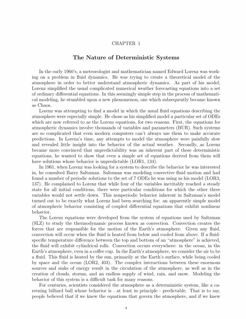
Unlike the billiard ball, the Earth’s atmosphere exhibits what is called a “sensitive de-pendence on initial conditions,” or SDIC. Systems that are deterministic, but which oftenappear to be random, are difficult to predict because the uncertainty in measurement willeventually result in a divergence between the system’s actual behavior and the model’s pre-diction thereof. “In some dynamical systems it is normal for two almost identical states tobe followed, after a sufficient time lapse, by two states bearing no more resemblance thantwo states chosen at random from a long sequence (LOR3, 8).” A simple example of SDICis given by the game Plinko, shown in figure 1, which is played on the television game show“The Price is Right.” In this game, contestants are given three plinko chips, which are

1. THE NATURE OF DETERMINISTIC SYSTEMS 6

shaped like hockey pucks. The chips are released adjacent to a vertical wall filled with pegswhich are offset from row to row. The pegs are designed to ensure that the plinko chiptravels a “random” path before landing at the bottom of the board, where a monetary valueis awarded.

Let’s assume a contestant on the game show drops her first plinko chip and it travels apath P1 down the board, landing in the $10,000 bin. With her second attempt, the contestantmight try to drop the plinko chip from the exact same location as the first chip. If she doesa good job of recreating the initial conditions of the first drop, the chip will probably bouncein the same direction after the first, second, and maybe even the third peg on the board.But no matter how vigilantly the contestant tries to recreate the chip’s motion, the pathP2 of the second chip will almost certainly be different from P1. For example, if the secondchip weighs a fraction of an ounce more than the first, or if the contestant’s thumb sticksto the chip for an extra fraction of a second, or if the spin on the chip is slightly different,the two paths can and will diverge from each other. The plinko game is a good exampleof a system that is deterministic, but whose behavior in practice is unpredictable becauseof its SDIC. The system is so sensitively dependent upon initial conditions that the tiniestdifference between drops will result in totally different trajectories.

Fortunately, there are a number of aspects of chaotic systems which are predictable andorderly. Despite the unpredictability of weather on a daily time scale, seasonal weatherpatterns are very orderly. Even when extreme weather conditions do arise, the Earth’satmosphere usually returns to more familiar weather patterns. Furthermore, while there areinfinitely many possible conditions of the Earth’s atmosphere, only a finite number of thesestates are physically meaningful. For example, the temperature of the water off of the coastof Maine will probably never top 100◦ F, despite the fact that such a condition is possible.The state of the atmosphere is bounded in a sense by those extreme weather conditionswhich rarely occur. The conditions towards which the Earth’s atmosphere is “attracted”form what is called an attractor. We will discuss the attractor associated with Lorenz’sconvection model later in this thesis.

Even simple systems like plinko can exhibit chaotic behavior, making predictions difficult.But by reducing complicated systems into simple ones through modeling, we can learn moreabout the different consequences resulting from the SDIC in each case. We now examine arelatively simple mathematical model of the atmosphere, and then describe an experimentbased upon it that can be used to illustrate some surprising effects that result from thesystem’s SDIC.

CHAPTER 2

The Lorenz Equations

Much of the emphasis on the Lorenz equations, in both differential equations textbooksand in the popular literature, is on the dynamics of the Lorenz system. Indeed, the Lorenzattractor and other properties of chaos predicted by the Lorenz equations are enough to fillan entire textbook. On the other hand, the derivation of the Lorenz equations is almost al-ways left as an exercise for the intrigued and mathematically experienced reader. Therefore,the mathematical development of the Lorenz equations from the equations of momentumand fluid flow is the subject of this chapter.

Temperature Deviation

As mentioned in Chapter 1, the Lorenz model is used to describe convective motion in afluid. The fluid is contained in a long, thin cell, bounded above and below by parallel plates.The top plate maintains a temperature Tc, while the bottom plate is held at a temperatureTw, where Tw > Tc. The temperature difference ∆T = Tw - Tc is fixed, but can be adjustedto create different types of behavior. The system is given by the fluid contained in the cell,heated from below by the hot plate and cooled from above by the cold plate. It was firststudied experimentally by Benard in 1900, and then theoretically by Lord Rayleigh in 1916(HLB, 29). As a result, this configuration is called a Rayleigh-Benard cell.

The convection cell is used to simulate the qualitative behavior of the atmosphere. Thesun heats the Earth’s atmosphere and surface, providing an enormous source of thermalenergy. The ocean and space siphon that energy out of the atmosphere. As this “tug ofwar” takes place, the air above the warm ground rises due to convection until it reaches thedew point where it condenses to form clouds. On the other hand, as the outermost layer ofthe atmosphere is cooled by space, it becomes more dense and falls. In this way convectioncurrents are created in the atmosphere, and we have weather (BUR, 12).

In a convection cell, if ∆T remains small, the fluid remains still, and the heat energyreleased by the bottom plate is absorbed by the pockets of fluid in the bottom of the cell.This heat is then transfered to the top of the fluid through thermal conduction. The densityof a small pocket of fluid decreases as the fluid is heated, so a pocket near the bottom plateexperiences a buoyancy force pushing upward. However, when the cell is in a conductivestate, the pocket of fluid loses heat to neighboring cool pockets before it has time to rise inthe cell. In such a situation, the temperature in the cell falls linearly with vertical positionfrom Tw at the bottom of the cell to Tc at the top (HLB, 29), see figure 2.

The temperature Td at any location (x, z, t) in the cell while the fluid is in a conductivestate, where no motion is present, can thus be described

(1) Td(x, z, t) = Tw −z

h∆T ,

where z is the vertical height in the cell measured from the bottom, x is the horizontalposition, and h, the height of the cell, is fixed. Because the cell is thin, the motion isessentially two dimensional, so there is no depth component in any of the functions concerning

7

2. THE LORENZ EQUATIONS 8

Figure 2. Conduction in a Rayleigh-Benard cell

the fluid flow. The temperature is assumed constant for all y values, or depths, of the cell. Aswe would expect, the boundary conditions ensure that at height z = 0 in the cell, Td(x, 0, t)= Tw for all values of x and t. At a height z = h, Td(x, h, t) = Tc. Finally, in the center of thecell at z = h/2, the linear function Td(x, h/2, t) gives us the average temperature betweenthe top and bottom plates.

When the temperature difference ∆T grows past a threshold value, the buoyancy forceon the pocket of fluid overcomes the viscous force and gravity, and the fluid pocket begins torise before it loses an appreciable amount of heat energy through conduction. Once the fluidhas risen into a region of lower temperature and higher density, the buoyancy force increases,because the pocket is less dense than its neighbors (HLB, 605). If the upward force is strongenough, the pocket of warm fluid will continue to move up faster than it can cool off. Risingpockets of warm fluid push their way to the top of the cell, displacing the cooler pockets offluid. These cooler pockets are more dense, and are pushed down towards the bottom of thecell. The process repeats itself causing convection rolls to appear in the cell, and the cell isthus in a convective state, see figure 3.

Let Tv(x, z, t) be the temperature of the fluid at a point (x, z) at time t, when it’s in aconvective state. We next define a function that measures the deviation of the convectivestate temperature Tv from the conductive state temperature Td. This deviation function isdefined as

(2) ϕ(x,z,t) = Tv(x, z, t)− Td(x, z, t),

and can be written as

(3) ϕ(x,z,t) = Tv(x, z, t)− Tw +z

h∆T .

Since the temperatures of the top and bottom plates are fixed, we expect that whenz = 0 and z = h, the convective state temperature Tv(x, z, t) will agree with the conductivetemperature function Td(x, z, t), and the deviation will be 0, ie. ϕ(x, 0, t) = 0 and ϕ(x, h, t)= 0 for all x and t. Notice that this means the temperature of the fluid at the very top andbottom of the cell is the same for both convection and conduction.

Navier-Stokes and Thermal Energy Equations

We now describe the relationship between the motion of a heated fluid and the forcesassociated with heating. The Navier-Stokes equations for fluid flow are often used to obtain


Figure 3. Convection cells

a quantitative description of fluid dynamics. Once again, convective motion is taken to beindependent of depth y in the cell, so only the horizontal and vertical components of thefluid velocity ~v are of interest. The two equations for conservation of momentum in a fluidare

ρ∂vz

∂t+ ρ~v · ∇vz = −ρg − ∂p

∂z+ µ∇2vz(4)

ρ∂vx

∂t+ ρ~v · ∇vx = −∂p

∂x+ µ∇2vx

In these fluid transport equations, ρ is the mass density of the fluid and is a function oftemperature, g is the acceleration due to gravity, p is the fluid pressure and is a functiononly of the height z, and µ is the fluid viscosity (HLB, 608). The vector representing thefluid flow velocity, ~v, is composed of velocity components vx and vz which are each functionsof x, z, and t. The first term on the left side of equation (4) accounts for the fact that themomentum of a pocket of fluid will change as the pocket accelerates. The second term showshow momentum changes as the pocket of fluid moves to an region where the momentumis different. This advection term is nonlinear in the velocity, and accounts for the chaoticbehavior of the system. The right side of equation (4) represents the sum of the forces actingon a small pocket of fluid. The three forces involved are gravity, fluid pressure, and viscosity.As one would expect, gravity has no effect on the x component of the fluid velocity.

The temperature of the fluid can be described by the thermal energy diffusion equation,satisfied by our convective temperature function Tv as follows

(5)∂Tv

∂t+ ~v · ∇ Tv = DT∇2Tv,

where DT represents the thermal diffusion coefficient. This coefficient depends on the typeof fluid and the viscosity of the fluid. If DT is large, then the fluid molecules will spreadout quickly as a result of heating (HLB, 509). The thermal diffusion equation gives usinformation about how heat energy is dispersed by a pocket of fluid, and in which direction.In order to find the thermal energy diffusion equation in terms of our temperature deviationfunction ϕ, we substitute Tv from equation (3) into (5), resulting in

(6)∂(ϕ + Td)

∂t+ ~v · ∇ (ϕ + Td) = DT∇2(ϕ + Td).


Since Td is independent of x and t, (6) reduces to

(7)∂ϕ

∂t+ ~v · ∇ ϕ− ~vz

∆T

h= DT∇2ϕ.

The mass density of the fluid, ρ, decreases as the fluid is heated and increases when thefluid is cooled. As a result, ρ is a function of the temperature Tv, which we will write interms of a power series expansion

(8) ρ(Tv) = ρo +dρ

dT

∣∣∣Tw

(Tv − Tw) + ...

where ρo = ρ(Tw). If we then define the thermal expansion coefficient α by

(9) α = − 1

ρo

dρ

dT

∣∣∣Tw

,

and substitute our temperature deviation function into the power series for ρ, the first twoterms become

(10) ρ(Tv) = ρo − αρo[ϕ(x, z, t)− z

h∆T ].

Only the first two terms in the power series for ρ(Tv) are shown in (10) because ofthe small variation in density throughout the fluid cell. This simplification, known as theBoussinesq Approximation, is valid for systems in which the variation in density is dueonly to small variations in temperature (CHN, 16). In other words, when the temperaturevariations throughout the cell are small, there is a negligible difference in volume expansion,on the order of 10−4. As a result, we can ignore all but the linear terms in the power seriesfor ρ(Tv).

In the Navier-Stokes equations (4), the Boussinesq Approximation further reduces thedensity variation by allowing us to substitute ρ(Tv) = ρo into all of the terms except the oneinvolving gravity (CHN, 16). For the term involving gravity, we insert the linear approxima-tion of ρ(Tv). The fluid pressure function p is then replaced by an effective pressure gradientfunction β which has the condition that β is a constant when the fluid is in a conductingstate (HLB, 609). In a convecting state, the pressure gradient is

(11) β = p + ρogz + αρogz2

2

∆T

h.

When we substitute the pressure gradient β into the Navier-Stokes equations, use theBoussinesq Approximation twice, and divide by ρo, we arrive at

∂vz

∂t+ ~v · ∇vz = − 1

ρo

∂β

∂z+ αϕg + ν∇2vz(12)

∂vx

∂t+ ~v · ∇vx = − 1

ρo

∂β

∂x+ ν∇2vx

where ν = µ/ρo is the kinematic viscosity, around 1.1 ∗ 10−5 m2/s for water (PAT, 133).Now that we have a form of the Navier-Stokes equations more specific to our two dimen-

sional cell, we need make only a few more transformations before we can attempt to find asolution. It will be more convenient when trying to understand the effect each parameterhas on the system if all of the variables are in a unitless form. To do this, we first define anew time parameter t′ as

(13) t′ =DT

h2t,

where h2/DT is a typical time for thermal energy to diffuse over a distance h (HLB, 610). Theunitless distance variables are defined as x′ = x/h and z′ = z/h. The unitless temperature


variable is defined as ϕ′ = ϕ/∆T . Based on these variables, the unitless velocity can thenbe defined as

vx′ =

DT

hvx(14)

vz′ =

DT

hvz

and the time independent, dimensionless Laplacian operator is then defined as ∇′2 = h2∇2.Using these new unitless variables and multiplying by a constant, we can rewrite the

Navier-Stokes equations (12) without the primes as follows

DT

ν[∂vz

∂t+ ~v · ∇vz] = − h2

νDTρo

∂p

∂z+α∆Tg

νDT

h3ϕ+∇2vz(15)

DT

ν[∂vx

∂t+ ~v · ∇vx] = − h2

νDTρo

∂p

∂x+∇2vx

Many significant ratios of parameters appear in the unitless form of the Navier-Stokesequations. As a result, some of them have been given names. The Rayleigh number R is animportant parameter describing the balance between the buoyancy force on a pocket of fluidas a result of thermal expansion with the loss of energy to thermal diffusion and viscosity(HLB, 611). It is a unitless parameter that can be adjusted by changing the temperaturedifference ∆T , and is important in determining the value of ∆T at which convection willbegin. It is defined as

(16) R = ∆Tαgh3

νDT

.

The Rayleigh number is the most important parameter of a fluid flow system and willbe discussed in more detail later. The second ratio is the Prandtl number σ which gives theratio of kinematic viscosity to the thermal diffusion coefficient (HLB, 611),

(17) σ =ν

DT

.

The Prandtl number compares the amount of energy lost to shearing of the fluid in motionwith the energy lost to conductive heat flow in the fluid (HLB, 611). If the Prandtl numberis greater than 1, the fluid loses more mechanical energy in motion than it does to heat flow.For example, water at room temperature has σ ≈ 7. Both the Rayleigh number, R, andthe Prandtl number, σ, are important parameters in the Lorenz system. Small adjustmentsin these parameters can turn a stable or periodic fluid flow into one which is turbulent orchaotic (GSN). The exact requirements of unstable flow will be discussed later.

The final dimensionless ratio Π is related to the pressure of the fluid and is defined to be

(18) Π =βh2

νρoDT

.

Using the unitless variables and the three ratios defined above, we can rewrite the Navier-Stokes equations (15) as

1

σ[∂vz

∂t+ ~v · ∇vz] = −∂Π

∂z+Rϕ+∇2vz(19)

1

σ[∂vx

∂t+ ~v · ∇vx] = −∂Π

∂x+∇2vx

Making the same substitutions, the thermal energy diffusion equation (7) becomes

(20)∂ϕ

∂t+ ~v · ∇ϕ− vz = ∇2ϕ.


It should be noted that by grouping together constants and functions into the parametersR, σ, and Π, we have not introduced any further simplifications to our model of convection.We are merely gathering together variables to create parameters with physical meaning.Equations (19) and (20) will be used to find a fluid streamfunction that describes the mo-tion of the fluid.

Fluid Streamfunction

The vector representing the fluid flow velocity, ~v = ~v(x, z, t), which appears in equations(19) and (20), can always be deduced from a fluid streamfunction Ψ(x, z, t). The stream-function supplies all of the important information about the fluid flow. At any time t, thefunction Ψ(x, z, t) provides the streamlines of the fluid motion (HLB, 493). The fluid velocityvector ~v is tangent to a streamline, with Ψ defined such that its gradient is perpendicular to~v according to the relations

vx = −∂Ψ(x, z, t)

∂z(21)

vz =∂Ψ(x, z, t)

∂x

The negative sign could be placed in front of either velocity component, but this choiceresults in the conventional Lorenz equations (HLB, 612). When we expand the gradient anddot product in equation (20), we get

(22) ~v · ∇ϕ = −∂Ψ

∂z

∂ϕ

∂x+∂Ψ

∂x

∂ϕ

∂z.

Inserting this term into (20), we find

(23)∂ϕ

∂t− ∂Ψ

∂z

∂ϕ

∂x+∂Ψ

∂x

∂ϕ

∂z− ∂Ψ

∂x= ∇2ϕ.

This equation is the first differential equation relating the streamfunction Ψ to the tem-perature difference function ϕ. The second differential equation is obtained by substitutingthe velocity components vx and vz into equation (19). The vx equation becomes

(24)1

σ[− ∂2Ψ

∂t∂z+∂Ψ

∂z

∂2Ψ

∂x∂z− ∂Ψ

∂x

∂2Ψ

∂z∂x] = −∂Π

∂x−∇2∂Ψ

∂z,

and the vz equation becomes

(25)1

σ[∂2Ψ

∂t∂x− ∂Ψ

∂z

∂2Ψ

∂x2+∂Ψ

∂x

∂2Ψ

∂z∂x] = −∂Π

∂z+Rϕ+∇2∂Ψ

∂x.

To eliminate the pressure related parameter Π, we take the partial derivative of (25) withrespect to x and subtract the partial derivative of (24) with respect to z. The result is

(26)1

σ

[∂

∂t(∇2Ψ)− ∂

∂z

(∂Ψ

∂z

∂2Ψ

∂x∂z− ∂Ψ

∂x

∂2Ψ

∂z2

)− ∂

∂x

(∂Ψ

∂z

∂2Ψ

∂x2− ∂Ψ

∂x

∂2Ψ

∂x∂z

)]= R

∂ϕ

∂x+∇4Ψ.

Equations (23) and (26) describe the motion and temperature of a fluid being heated.They couple the behavior of our functions Ψ(x, z, t) and ϕ(x, z, t).

Truncation and Numerical Analysis


We will now find functions Ψ and ϕ that satisfy our set of differential equations, alongwith the appropriate boundary conditions. The boundary conditions for ϕ were discussedpreviously, after we defined ϕ in equation (3). The boundary conditions for Ψ will be satisfiedif the partial derivatives in equation (21) satisfy the requirements of convection. We wouldexpect the vertical component of the velocity vz to be zero at the top, z = 1, and bottom,z = 0, of the cell. Similarly, the horizontal component of the velocity vx should be zero atthe sides of the cell.

One common technique for finding solutions to a differential equation is to first find asolution that is separable. A separable solution in this case is a function that is the productof three component functions, one for each variable x, z, and t. Consider a solution of theform

(27) Ψ(x, z, t) =∑m,n

eωm,nt[Amcos(λmz) +Bmsin(λmz)] · [Cncos(λnx) + Dnsin(λnx)]

where each λ is the wavelength of a Fourier spatial mode. The spatial modes depend onthe dimensions of the convection cell and are chosen to ensure that the solution satisfiesthe boundary conditions. Each λ has a corresponding frequency ωm,n which determines howoften the magnitude of the function oscillates (HLB, 614).

Equation (27) is an infinite sum of sine and cosine terms. To make the general solutionsimpler, the sum is truncated using a process called the Galerkin procedure (HLB, 614). Wemight be concerned that in approximating the equations for Ψ and ϕ we will lose much ofthe important nonlinear nature of the system. Fortunately, Saltzman has shown numericallythat this truncation still captures most of the important nonlinear behavior (SLZ). Usingthe Galerkin procedure, we choose a finite number of sine and cosine terms from the Fourierexpansion of Ψ. A similar Fourier expansion and Galerkin truncation also results in a generalsolution for ϕ. The resulting sum of the truncated equations for the fluid streamfunctionand temperature deviation function are

(28) Ψ(x, z, t) = ψ(t)sin(πz)sin(ax)

(29) ϕ(x, z, t) = T1(t)sin(πz)cos(ax) − T2(t)sin(2πz),

where the height of the cell is taken to be 1 so that z ∈[0,1]. The parameter a is chosen sothat the Rayleigh number is at its minimum when convection begins, and will be discussedin more detail later.

The time dependency of Ψ(x, z, t) and ϕ(x, z, t) is represented by ψ(t), T1(t), and T2(t)which are unknown functions whose roles in the streamfunction and temperature deviationfunction we will now discuss. The T1 term in the temperature deviation function gives thetemperature difference between the upward and downward currents in the convection cell.The T2 term gives the deviation from the linear temperature variation in the center of thecell as a function of z (HLB, 615). Without the T2 term, the temperature deviation functionwould not capture the effect of circulation on the diffusion of heat energy.

To see how well the solutions given by (28) and (29) describe convection in a Rayleigh-Benard cell, we will check the boundary conditions. For the streamfunction, we must seethat the vertical component of the velocity, vz, is zero at the top and bottom of the cell.Similarly, the horizontal component of the velocity, vx, should be zero at the sides of the


cell. These boundary conditions are easily checked

vz(x, 1, t) =∂Ψ(x, 1, t)

∂x= aψ(t)sin(π)cos(ax) = 0(30)

vx(π

a, z, t) = −

∂Ψ(πa , z, t)

∂z= −πψ(t)cos(πz)sin(π) = 0

For the temperature deviation function, we would expect from equation (3) that thedeviation at the top and bottom of the cell is zero. This is easily checked in a mannersimilar to that above. Along the z = 1/2 horizontal axis, where 0 < x < π/a, the T2(t) termvanishes and we are left with ϕ = T1(t)cos(ax). The temperature deviation is maximized at(0, 1/2, t) where ϕ is reduced to ϕ(t) = T1(t). This position will be known as 9 o’clock in asingle convection cell. Likewise, the temperature deviation is most negative at (π/a, 1/2, t)or 3 o’clock, where ϕ(t) = -T1(t). In the very center of a convection cell, at (π/2a, 1/2, t),the temperature deviation from linear is 0.

Along the x = π/2a axis, the T1(t) term disappears and we are left with ϕ(t) = -T2(t)sin(2πz). Then for 0 < z < 1/2, ϕ(t) = -T2(t)N where both N and T2 are positive.This implies that any pocket of fluid below z = 1/2 on the x = π/2a axis is cooler thanpredicted by a linear temperature variation. Likewise, for 1/2 < z < 1, ϕ(t) = T2(t)N . Thisimplies that a pocket of fluid above z = 1/2 on the same axis is warmer than it should be.Both these implications are consistent with our understanding of how a pocket of fluid willmove when it exhibits convection rolls. A warm pocket of fluid below z = 1/2 will rise inthe cell, displacing a cold pocket somewhere above z = 1/2. Once the warm pocket reachesthe upper half of the cell, it is warmer than predicted by the linear temperature functionassociated with conduction (1). Consequently, ϕ will return a positive number, indicatingthat the convecting pocket of fluid is warmer than a conducting pocket would be.

Lorenz Equations

To obtain the final form of the Lorenz equations, we substitute our expressions for Ψ,(28), and ϕ, (29) into the differential equations (23) and (26). The result is simplified bythe following relations for the time independent Laplacian operator

∇2Ψ = −(π2 + a2)Ψ(31)

∇4Ψ = (π2 + a2)2Ψ

Inserting the solution functions (28) and (29) into equation (26) gives

(32)−dψ(t)

dt(π2 + a2)sin(πz)sin(ax) = −σRT1(t)sin(πz)sin(ax)

+ σ(π2 + a2)2ψ(t)sin(πz)sin(ax).

When we equate the coefficients of the sin(πz)sin(ax) terms, the result is

(33)dψ(t)

dt=

σR

π2 + a2T1(t)− σ(π2 + a2)ψ(t).


When we substitute the proposed solution functions Ψ and ϕ into equation (23), we find

(34)dT1

dtsin(πz)cos(ax)− dT2

dtsin(2πz) + (π2 + a2)2T1sin(πz)cos(ax)

− 4π2T2sin(2πz)− ψasin(πz)cos(ax)

= −[ψπcos(πz)sin(ax)][T1asin(πz)sin(ax)]

− [ψasin(πz)cos(ax)][T1πcos(πz)cos(ax)]

+ [ψsin(πz)cos(ax)][2πT2cos(πz)cos(ax)].

Many of the terms in equation (34) have sin(πz)cos(ax) in them. If we equate theseterms, dropping one term whose spatial dependence is beyond the scope of our model (HLB,616), we are left with

(35)dT1(t)

dt= aψ(t)− (π2 + a2)T1(t)− πaψ(t)T2(t).

The other terms in the temperature deviation equation (34) are multiplied by sin(2πz).Equating these terms we have

(36)dT2(t)

dt=πa

2ψ(t)T1(t)− 4π2T2(t).

These three equations, (33),(35), and (36), relate the time dependent part of the stream-function, ψ(t), to the temperature gradient functions T1(t) and T2(t). They are the threedifferential equations describing all motion in the Lorenz system. To obtain the final formof the Lorenz equations, we make a few more substitutions. We introduce the new timevariable

(37) t′ = (π2 + a2)t,

and the reduced Rayleigh number r

(38) r =a2

(π2 + a2)3R.

The reduced Rayleigh number is defined so that when r ≤ 1, the fluid is in a conductiveor stable state. So for our discussion, r > 1 implies that the fluid will start rolling. Thismeans

(39) R ≥ (π2 + a2)3

a2

is the condition necessary for convection.The parameter a is related to the width of the convection cell in the x-direction. We

choose a = π/√

2, so that R is as small as possible while still satisfying Equation (39).Physically, this means that for a cell with height 1, convection rolls will begin to appearwhen the horizontal width of the cell is chosen to be greater than or equal to

√2. Any

smaller value for a would restrict the fluid in the cell from exhibiting convection rolls. Anylarger value for a would merely complicate our model. This choice for a gives the Rayleighnumber at which convection begins, R = 27π4/4 (HLB, 618).

Finally, the parameter b is defined as

(40) b =4π2

π2 + a2,

where the condition for convection, a = π/√

2, gives us a value of b = 8/3.


Figure 4. Lorenz Attractor

We will also rename ψ, T1, and T2 with the new time variable as follows

X(t) =aπ

(π2 + a2)√

2ψ(t)(41)

Y (t) =rπ√

2T1(t)

Z(t) = rπT2(t)

Taking these definitions for X, Y, and Z, and substituting them into equations (33), (35),and (36), we arrive at the final form of the Lorenz equations

dX

dt= σY (t) − σX(t)(42)

dY

dt= rX(t) − X(t)Z(t) − Y (t)

dZ

dt= X(t)Y (t) − bZ(t)

These equations are used to study one of the most mathematically complicated objectsever discovered, the Lorenz attractor. The Lorenz attractor, often called the “butterfly”attractor because of its wings, is the shape associated with every initial condition of theLorenz equations. The trajectory never intersects itself, despite coming arbitrarily close.An example of the Lorenz attractor is shown in figure 4. The solution curve for the initialcondition (0, 9, 3) is traced out by the Lorenz equations in three dimensional phase space.The behavior of the trajectory is far more interesting when viewed in real time while theattractor is being drawn. The solution loops around two foci, located at (6

√2, 6

√2, 27)

and (-6√

2, -6√

2, 27), like a planet orbiting two suns. The “gravitational” pull of one focuswill only dominate the trajectory for a short time before it is tugged away by the pull of theother.

As we shall see, the behavior of the solutions to this set of coupled differential equationsis extremely complicated and beautiful. However, their development is very rarely men-tioned in any of the mathematics texts which discuss the Lorenz system. This could be aresult of the difficulty mathematicians have in justifying the approximations and truncationsrequired by the derivation. Fortunately, Lorenz wasn’t looking for an exact description ofthe fluid flow in Rayleigh-Benard convection. He was merely trying to find a simple systemof equations to illustrate numerical weather forecasting. In developing the equations, he“proceeded in the manner of a professional meteorologist and an amateur mathematician”


(LOR3, 132). If he hadn’t made so many approximations in his paper Deterministic Nonpe-riodic Flow (LOR1), Lorenz may never have discovered this system. Unfortunately for thegeneral scientific community, he published in the Journal of the Atmospheric Sciences. As aresult, it took almost a decade for the physics and mathematics communities to realize whathe had discovered.

CHAPTER 3

A Simple Model of the Weather

Very few attempts have been made to design an experimental apparatus demonstratingthe type of behavior predicted by the Lorenz equations. This is surprising considering howimportant the effects of Lorenz type chaos might be in weather prediction. By studying thedynamics of the Lorenz equations in an actual convection experiment, we expect to acquiremore insight into the type of phenomena they predict, and some insight into how they mightbe used to improve our ability to forecast the weather.

Thermosyphon

One simple model of convection in the Earth’s atmosphere is the thermal convectionloop, or thermosyphon. The thermal convection loop is a torus shaped tube, filled withfluid, standing in the vertical plane. The bottom half of the tube is heated at a constant ratewhile the top half is cooled at a constant rate. The circular geometry of the thermosyphonis chosen in order to force the fluid to exhibit mathematically convenient circular convectionrolls. Thermocouples are inserted into the tube at 3, 6, and 9 o’clock on the face of the loopto measure the temperature of the fluid at each position (labeled B, C, and A respectivelyin Figure 5).

The thermocouples are inserted as close to the center of the tube as possible to avoidmisleading readings, since the behavior of the fluid is not uniform across the entire diameterof the tube. Furthermore, by taking measurements of the temperature near the center, weavoid complications which arise near the boundary.The temperature sensor at point C is used to find the average temperature of the fluid inthe bottom half of the tube at any given time. The sensors at points A and B are used toestablish the temperature difference during convection between the warm, rising fluid andthe cool, falling fluid. The temperatures at points A and B will be labeled TA and TB. Thedifference between the temperatures at these two points is an important quantity, and isdefined to be

(43) δT = TA - TB.

The temperature at point C will be called Tw, corresponding to the temperature of the lowerplate in the Rayleigh-Benard convection cell model.

The fluid in the thermosyphon is initially at rest, with the heat energy from the bottomhalf of the tube being transfered to the top half by conduction. The fluid in the tube willbegin to rotate when the temperature difference between the top and bottom halves of theloop is great enough to create the density variation required for buoyancy to overcome gravityand viscosity (HLB, 605). Fluid in the top half of the loop is cooled, making it heavier andmore likely to sink. Fluid in the bottom half of the loop is heated, making it less denseand more likely to rise. Consequently, the fluid will eventually begin to circulate around thetube.

18

3. A SIMPLE MODEL OF THE WEATHER 19

Figure 5. Thermal Convection Loop

When the heating and cooling rates are held constant, an initially stationary fluid willaccelerate until the effects of buoyancy and friction balance each other out (CRV, 65). Oncean equilibrium is achieved, the fluid flow rate should be constant in both magnitude anddirection, a steady state. However, under certain conditions, a steady state is never reachedby the fluid in a thermal convection loop. When the temperature difference between thetop and bottom halves of the loop is within a particular range, the fluid oscillates in anunstable and chaotic manner. The stable and unstable states of fluid oscillation in a thermalconvection loop are the topic of this chapter.

Theory

The theoretical predictions that have been made concerning thermosyphons are all de-pendent upon the heating and cooling rates used to force convection in the fluid. Ourexperimental apparatus uses the air at room temperature to cool the fluid rather than acoolant filled sleeve. The resulting behavior is the same as long as a large enough δT iscreated. Consequently, we will only discuss the theoretical predictions regarding the heatingrate, since the cooling rate is relatively constant.

At the beginning of each trial, a heating rate V is chosen to heat the bottom half ofthe tube. This rate remains unchanged throughout each experimental trial. When the heatsource is switched on to supply V , the heat energy initially conducts up through the fluidfrom the bottom of the tube to the top. Small pockets of fluid lose heat to neighboringpockets before they have time to rise. During this initial conduction stage, the temperaturethroughout the entire tube rises slowly. This conduction stage continues until the threshold


temperature for convection is reached. For any heating rate V < Vi, the threshold tempera-ture is never reached. The heating rate V is not strong enough to force the fluid to convect,so the fluid remains motionless. Conduction slowly warms up the fluid throughout the tube,but no rotational motion occurs.

For heating rates of V > Vi, the initial conducting state of the fluid changes to a con-vecting state within minutes. The direction in which the fluid begins rotating is determined,but in reality it is impossible to predict, much like the flip of a coin. In a stable state ofthe convection cell, once the fluid has chosen a direction in which to rotate, be it clockwiseor counterclockwise, that direction will remain unchanged as long as the conditions underwhich it was produced are unchanged.

The onset of convection can be observed by watching the temperature difference δTdescribed in equation (43). If |δT | > 0, the temperature is greater on one side of the tubethan the other, and the fluid has begun to rotate. For example, if δT = TA - TB is less thanzero, then we know the temperature of the water is greater at point B than at point A andthe fluid must be rotating in a counterclockwise direction. The logic behind this assertion isas follows.

Assume the water in the tube has begun to rotate in a counterclockwise direction, asin figure 5. A pocket of fluid beginning near point A on the loop at time t1 is constantlyheated as it travels around the bottom half of the loop, past point C. By the time the pocketof fluid reaches point B, it has experienced the maximum amount of heating that the heatsource has to offer. At that moment, time t2, it is the hottest pocket in the entire tube.Now imagine the pocket of fluid which begins just above point B at time t1, antipodal tothe pocket just discussed. This pocket is constantly cooled by the air in the lab as it rotatesalong the top half of the loop from point B to point A. When it reaches point A at time t2,it has experienced the maximum amount of cooling that the air in the lab has to offer. As aresult, it is the coolest pocket of fluid in the entire tube. Since these two antipodal pocketsof water reach points A and B at the same time t2, their difference in temperature is a directindication of the direction of rotation of the fluid.

Conversely, if the fluid initially begins to rotate in a clockwise direction, the temperatureat point A will always be greater than the temperature at point B by the same argument,and the fluid will continue to rotate in a clockwise direction. Clockwise rotation results in ameasurement of δT = TA - TB greater than zero.

The work done by Creveling et.al. indicates that there is a distinct range of values forthe heating rate V under which the thermosyphon remains in a stable state (CRV). In otherwords, for heating rates V within the range Vi < V < Vcrit, the fluid in the tube rotates inonly one direction from the moment conduction gives way to convection until the heat sourceis turned off. With the heat source set to supply any V in this range, the future behaviorof the system is thus very predictable. If the transient behavior dies out at time ti, and thesystem reaches a balance or equilibrium between the heating and cooling of the tube, we canaccurately predict the direction of rotation with no uncertainty, as well as the temperaturedifference δT , from ti to any later time t. The velocity of rotation and the temperaturedifference δT are virtually constant for any heating rate V within the stable range.

For heating rates within the stable range, weather forecasting in our thermosyphon is easy.Given the current state of the system, defined by V and δT , any future state of the systemis unchanged once transient behavior dies out. However, this ability to predict the weatheris lost once the heating rate is increased outside the stable range. For V > Vcrit, the fluidnever reaches a stable state. After the transient behavior dies out, the fluid will oscillate in achaotic manner, changing from clockwise to counterclockwise rotation at irregular intervals.Any attempt to predict the future state of the system, δT , based on the current δT will result


in an exponential growth in uncertainty. This growth in uncertainty is common to all chaoticsystems which exhibit the sensitive dependence on initial conditions that was discussed inChapter 1. The chaotic behavior of the fluid in the thermosyphon illustrates complicationsthat could very well occur when trying to forecast weather in the Earth’s atmosphere. Thesame effects are thought to be responsible for the periodic inversions of the Earth’s magneticfield, as well as the periodicity in the motion and size of sunspots, which are related to thesun’s magnetic field.

Experimental Apparatus

The thermal convection loop for this experiment was constructed out of transparentplastic tubing with a melting point of 180 degrees Fahrenheit. The inner diameter, of thetube is 1 inch, with a wall thickness of 3

16of an inch. The loop is supported vertically in

a circular shape of radius 13 inches. The fluid used to fill the tube, and model the air inthe Earth’s atmosphere, is water taken from the tap. Two holes were drilled in the jointconnecting both ends of the tube, to allow for colored dye to be added to the water for visualanalysis.

The top half of the tube is cooled by the room temperature air in the lab, ≈ 70◦ F.The bottom half of the loop is heated by heating tape connected to a Variac which can pro-duce temperatures between 70◦ and 450◦ F. Two lengths of heating tape are wound tightlyaround the tube in an attempt to create a constant and uniform heat source along its wall.The Variac allows for small adjustments in the amount of heat energy being transmittedto the water in the bottom half of the tube. The ability to accurately adjust the heatingrate parameter is crucial to modeling chaotic behavior in the atmosphere. The temperaturedifference δT = TA - TB is measured a few times each second by a digital dual channelthermometer, and recorded manually every 15 seconds.

Observations

As mentioned before, past research on thermal convection loops predicts that there arethere are two important values of the heating rate V : the rate at which conduction gives wayto convection, Vi, and the rate at which stable convection gives way to unstable convection,Vcrit. For our apparatus, the heating rate V corresponds directly to the power V the Variacsupplies to the heating tape. The direct proportion relating V and V has been not beenestablished, so to avoid confusion we will use V when referring to both the heating rate andthe Variac power. In what follows, we characterize the power supplied by the Variac in termsof the settings on its adjustment dial, which are given in Volts.

Experimental trials show that Vi ≈ 5 Volts for our thermosyphon. This means the waterin the tube remains motionless for any trial with V < 5 Volts. Conductive behavior isobserved numerically by the digital thermometer which reads δT = 0 even as the water inthe tube heats up.

For heating rates above 5 Volts, the decrease in density of the warm pockets of fluidresults in a buoyant force greater than the sum of the forces from gravity and viscosity,causing convection. Because of the geometry of the thermal convection loop, the fluid isforced to rotate rather than to simply rise and mix. Even though it can, in principle, bedetermined, we do not attempt to predict the direction in which the fluid will begin to rotate.


Figure 6. 20 Volts, 90◦ F at 6 o’clock

However, once the fluid has begun to rotate for some V in the range Vi < V < Vcrit, it willmaintain that direction of rotation “forever.”

We now look at experimental results in the form of a graph of δT versus time. It isimportant to note that the initial time on the graph, t = 0 minutes, is not the time at whichthe Variac is turned on. For all of the experimental trials, the tube is given time to come toan overall average equilibrium temperature. If we took data immediately after the heatingbegan, it would be difficult to reproduce. For small values of V , below 10 Volts, the timeallotted for transient behavior to die out is around 2 hours. For values of V > 10 Volts, thetube needed up to 24 hours to achieve an equilibrium temperature.

A plot of δT verses time is shown in figure 6 for the heating rate corresponding to V= 20 Volts. The temperature difference is measured in degrees Fahrenheit, while time isplotted in minutes. The title of the plot states that the temperature at point C on thethermosyphon, or 6 o’clock on the face of the loop, was 90◦ F. This value is taken to be theaverage temperature of the bottom half of the loop, and corresponds to Tw in Chapter 2.

There are a few interesting facts that can be observed in this graph. First, δT > 0 for theduration of the experiment, which means that the fluid was always rotating in a clockwisedirection. While data was only taken for 30 minutes, the stable nature of the system ensuresthat clockwise rotation would continue for as long as desired. Secondly, δT is relativelyconstant, oscillating slightly near 2◦ F. This means that the temperature TA at point Ais always about 2◦ warmer than TB at point B. Since the fluid is incompressible, we canconclude that the velocity with which the fluid is rotating is very nearly constant as well.We can confirm this by injecting a spot of food coloring dye into the rotating water andtiming its trip around the tube. Finally, and most importantly, we can predict the futurestate of the thermosyphon with very little uncertainty. That is to say, we know δT ≈ 2◦ ∀t.The system is in a stable state and “weather forecasting” in our thermal convection loop iseasy.

Figure 7 shows the results of an experimental trial with a heating rate of V = 49 Volts.At this rate, the temperature at point C is near 169◦ F. The graph looks very similar tothe one shown previously for V = 20 Volts. The water in the tube is flowing in a clockwisedirection with δT ≈ 2 degrees. Once again, the future state of the thermosyphon, and thus




the future state of the “weather” in the tube, is very predictable. It should be noted herethat for heating rates above V = 49 Volts, the heating tape is in danger of melting the plastictube, since the melting point of the tube is 180◦ F. In hopes of finding the heating rate atwhich the system behaves chaotically, Vcrit, one final trial was attempted with a heating rateof V = 50 Volts. Fortunately, the God that doesn’t play dice has a sense of humor. Theplot of δT verses time for this heating rate is shown in figure 8.

There are many interesting and important things to notice in the plot of δT for V =50 Volts. First, increasing the heating rate V by one volt has increased the temperatureat point C by only 3◦ F, from 169◦ to 172◦. But this very small change in the heatingrate, and consequently the overall average temperature, has turned a stable and predictablesystem into a chaotic and unpredictable one. We have found that Vcrit = 50 Volts for our



thermosyphon. Secondly, at the onset of the collection of data, the water in the tube isrotating in a counterclockwise direction, since δT < 0. Then 22.5 minutes later, the waterspontaneously switches its direction of rotation, and begins to rotate in a clockwise manner.This result is surprising, considering how stable the system was when the heating rate wasone volt less. It is also surprising considering the fact that the thermosyphon was allowed 24hours to come to equilibrium before this data was taken. This result is very counterintuitive,but the reversal of flow was also observed visually when colored dye was dropped into thefluid at the joint in the open part of the tube.

Another intriguing aspect of the experiment illustrated by the plot is the oscillation inamplitude of δT . During the first 10 minutes of the trial, δT is oscillating around δT = −2◦

F, between −1◦ and −3◦. This amplitude increases as time passes, to the point where δT isoscillating between 0◦ and −4◦. Once this minimum value of δT is reached, the fluid switchesits direction of rotation and begins to increase its amplitude of oscillation in a similar fashionas before. After t = 22.5 minutes, δT oscillates around +2◦ F.

It is clear that the values of δT around which the temperature differences oscillate are +2◦

and −2◦. However, +2◦ and −2◦ are also the values of δT measured for experimental trialswith V < 50 volts. This is unlikely to simply be a coincidence, but there is no theoreticalprediction in any literature that predicts this will occur. The increase in oscillation amplitudeis the one predictable behavior of the thermosyphon in a chaotic state. Further trials revealthat once the amplitude of δT reaches an absolute value above ≈ 4◦ F, the water in the tubeswitches its direction of rotation. Recent studies by Dr. Eugenia Kalnay at the Universityof Maryland indicate that the Lorenz state variables give a similar indication of the onset ofa flow reversal.

The trial shown in figure 9 is a good illustration of the predictability of a switch in flowdirection once a |δT | > 4◦ F is reached. This trial was also done with a heating rate Vcorresponding to 50 Volts. In the first 15 minutes that data was taken, the water in thetube changed its direction of rotation 6 times! Then for the second half of the experiment,the water rotated in a clockwise direction, with δT constantly increasing its amplitude ofoscillation. The spontaneous reversals of flow in the first half of the trial are not the result ofperturbations or forces outside of those mentioned already. The behavior is simply chaotic.


Figure 10. Anomoly generating flow reversal

It must be noted that the experimental results of Creveling indicate the existence ofanother important range in the heating rate V (CRV). For heating rates above some Vs, thefluid in the thermosyphon becomes stable again. That is to say, for V > Vs, the fluid inthe tube behaves like it did for heating rates V < Vcrit, rotating in one direction forever.Also, the direction of rotation remains stable until the heating tape nears the boiling pointof the fluid. When the boiling point is near, the fluid becomes increasing turbulent and failsto model convection in the atmosphere. Unfortunately, due to the limitations of the plastictubing we used to build our thermosyphon, Vs was never found since V > Vcrit = 50 Voltsmelted the plastic and destroyed the apparatus!

Before we begin our discussion of how the Lorenz equations relate to the thermosyphonexperiment, we present a physical explanation of the flow reversals. Assume the flow iscounterclockwise and that an anomolous ’hot’ pocket of fluid arrives at point B in the tube,figure 10. Due to some instability in the heating flux across the bottom half of the tube,this pocket is hotter than it should be. The hot pocket exerts a buoyancy force on thefluid, causing a positive acceleration in the counterclockwise direction and speeding up therotation, arrow a. This pocket cools less on its journey across the top half of the tube,arriving at point A hotter than it should be. Consequently, there is a buoyancy force in theclockwise direction acting to slow down the speed of rotation, arrow b. The fluid decelerates,allowing the anomolous pocket more time to heat up as it passes point C. Upon arriving atpoint B, the pocket is once again hotter than it should be, by a greater amount now thanbefore. The buoyancy force acting to accelerate the flowrate is greater this time since theinstability has been magnified, arrow c. With even less time to cool off, the pocket crosses thetop half of the tube to point A. The instability continues to grow, decelerating the clockwiseflow again, arrow d, accelerating the flow, arrow e. This amplification will continue until thebuoyancy force generated by the pocket at point A grows large enough, causing the flow to


stop. With no rotation in the tube, the temperature gradient between the top and bottomportions of the fluid grows unchecked. The fluid then reverses the direction of rotation, andthe behavior observed in figures 8 and 9 continues indefinitely.

The magnification of thermal instabilities is only observed at values of the heating pa-rameter above Vcrit. We conclude that this is a bifurcation value of the system. For V <Vcrit, we observe periodic rotation. For V > Vcrit, we observe chaos. The periodic behaviorfound for V < Vcrit may be due to some natural dampening of low energy systems.

CHAPTER 4

The Lorenz Attractor

The state of the “weather” in our thermosyphon, for any pocket of fluid, is describedby the pocket’s position, temperature, and velocity. In other words, knowing these threevariables at any particular time is all that is needed to know them at any future time, andhence to forecast the state of the system at any future time. Unfortunately, we were unableto measure the velocity of the fluid in our thermosyphon. We were only able to measure thetemperature difference between the warm rising fluid and the cool falling fluid on oppositesides of the tube. However, a technique known as state reconstruction can be used to un-cover more information about the shape of the Lorenz-like attractor which corresponds tothe behavior of the fluid in our thermosyphon.

State Reconstruction

Given a time series (a plot of a system measurement versus time), state reconstructionallows us to recover information about the system which we were unable to measure directly(ALL, 538). To see how, first recall that the temperature difference between the warm risingfluid and the cool falling fluid in a convection cell can be modeled using the function Y (t)defined in Equation (41), Chapter 2. No explicit solutions for the function Y (t) have beenfound, but numerical solutions to the Lorenz equations reveal the qualitative similaritiesbetween the behavior of Y (t) and that of the fluid in the thermosyphon.

For a certain initial condition, figure 11 shows the time series of the function Y (t) whosederivative is determined by the Lorenz equations. Compare this plot to that of the tem-perature difference measured experimentally with the thermosyphon for a heating rate of50 Volts in figures 8 and 9. Much of the qualitative behavior of the function Y (t) agreeswith the experimental results, most notably the increase in oscillation amplitude prior toa reversal of flow. As a way to see how well the Lorenz equations describe the behaviorof the fluid in our thermosyphon, we reconstruct the Lorenz attractor from the time seriesdescribed in Chapter 3. To do this, we plot each measurement of the time series of tempera-ture difference, δT (defined in Chapter 3), versus a time-delayed version. That is, given themeasured value of δT at a time t, we find δT at a time (t - τ) where τ is called the delay.This allows us to determine whether δT is increasing or decreasing at time t.

We then plot δT (t) versus δT (t - τ) and create a delay portrait for the temperaturedifference in the rotating fluid. If the behavior of the fluid were periodic, then the delay plotwould appear as a closed loop in phase space. Since we know the behavior of the rotatingfluid is not periodic for the thermosyphon, we don’t expect the delay plot to be a closedloop. The choice of τ is crucial to being able to construct an accurate delay plot. If τ is toosmall, the behavior of δT won’t have had time to change significantly from time (t - τ) totime t. As a result, the delay plot would appear almost like a plot of y = x, because δT (t- τ) ≈ δT (t). If τ is chosen too large, then much of the important behavior of the functionδT (t) might be missed. For example, if the data we are attempting to create a delay plotfor has many local maxima and minima, as our data does, a large τ might result in δT (t -

27

4. THE LORENZ ATTRACTOR 28

Figure 11. State variable Y, time series plot

τ) ≈ δT (t) even when a peak or valley has occured at some time between (t - τ) and t. Thepeak or valley would be ignored in the delay plot because τ was too large.

The delay portrait we create by plotting δT (t) versus δT (t - τ) can also be ambiguouswhen the two functions map to the same point in phase space at two or more different times.If we follow a trajectory through the phase space created by the delay plot by allowing timeto pass, and we reach an intersection in the trajectory, we will be unable to determine thedirection in which to travel. To attempt to resolve the difficulty, we add a third dimensionto our delay plot. If there are no self-intersections in three space, the implication is thatknowing the three values at any time t would be enough to say what happens next. In sucha case, there would only be one direction to travel along the trajectory at any point in time.For the Lorenz equations, the third dimension in our phase space is recovered by creatinga third function, δT (t - 2τ). If we then plot the three functions together, [δT (t), δT (t - τ),δT (t - 2τ)], we create an approximation of the Lorenz attractor (ALL, 547).

We now reconstruct the two dimensional Lorenz attractor from our thermosyphon mea-surements of δT , taking τ = 15 seconds to be the time delay. This τ is necessarily largebecause data was only taken every 15 seconds. Figure 12 plots the measurements of δT takenover the course of an hour. The two-dimensional delay reconstructed attractor for our datais shown in figure 13. In this reconstructed phase plot, points are plotted every 15 secondsand joined by straight line segments to make their progression easier to follow.

Consider now, plotting δT versus δT (t - 15s) versus δT (t - 30s) in three space. This willgive us a three dimensional phase portrait of the behavior of the fluid in our thermosyphon,figure 14. Note how the three dimensional plot appears to have a shape similar to that of theLorenz attractor. While the nature of the attractor is far more apparent when viewed as thepicture is created, the state reconstruction is successful in recovering the Lorenz attractorfor our thermosyphon data. In particular, there don’t appear to be any self intersections. In


Figure 12. Raw Delta T data

Figure 13. Two-dimensional delay reconstruction


Figure 14. Three-dimensional delay reconstruction

other words, no single data point seems to have four line segments meeting at it, indicatingthat knowing δT , δT (t - 15s), and δT (t - 30s) exactly at any time t allows for prediction offuture states.

Cubic Splines and a Smooth Attractor

The temperature difference data δT was only taken every 15 seconds. As a result, thereconstructed attractor for our thermosyphon has a number of jagged edges. To remedythis, we smooth the data in our time series plot of δT , and examine the consequences of thissmoothing on the state reconstruction plots.

While our data was only taken every 15 seconds, the actual behavior of δT was changingcontinuously. Plots of data collected more frequently would produce smoother curves. Forthe collection of 15-second time intervals between data points, we use a technique known ascubic spline interpolation to find cubic polynomials that have the same values as our data overeach time interval, and use them to smoothly connect each consecutive pair of data pointswith the proper inflection (KIN, 317). In a sense, the cubic spline fills in or interpolates thevalues of δT which we would have otherwise measured directly. For our 242 data points,we find 241 separate cubic splines to draw a smooth graph. Fortunately, computers can beprogrammed to find the necessary cubic polynomials so we don’t need to find all 241 byhand! The resulting time series of δT , smoothed using cubic spline interpolation, is shownin figure 15. Only a segment of the data is shown, with the raw data shifted 2 units up.

With this smoother time series, we again reconstruct the Lorenz attractor for our ther-mosyphon. Since the cubic spline allows us to pretend we have continuous data, we canchoose a more appropriate value for the time delay τ . For the shape of the time series, we


Figure 15. Segment of smoothed data

choose a value of τ = 1.5 seconds, one-tenth of our original value. We tried smaller valuesof τ and as expected they resulted in delay plots very close to the line x = y = z.

Now that our time series looks more like numerical approximations of Y (t), we plot thethree functions δT (t), δT (t - τ), and δT (t - 2τ). The resulting “smoothed” and reconstructedattractor for our thermosyphon data is shown in figure 16. Here we are using a delay of 3seconds, compare with figure 14 which used raw data and a delay of 15 seconds.Notice how the attractor in figure 16 appears to be “thinner” than that in figure 14, createdwithout the help of cubic spline interpolation. This is a drawback to state reconstruction,due to the sensitivity in the choice of τ . As mentioned before, if τ is small, the values ofδT (t), δT (t - τ), and δT (t - 2τ) will be very close, resulting in a curve lying very close to theline x = y = z. This makes the absence of self-intersections less clear, which is unfortunate,since a lack of self-intersections is what we need in order to know that values for δT (t), δT (t- τ), and δT (t - 2τ) are enough to determine any future state.

Ross Reconstruction

In an attempt to resolve the problems created by the time delay τ in delay plot recon-struction, we develop a new way to reconstruct the Lorenz attractor. Rather than plottingdata points as a function of previous data points, we plot data points versus the rates ofchange of the function in question at the same time. In other words, to reconstruct theLorenz attractor for our function Y (t) from Chapter 2, we plot Y (t) vs. Y ′(t). In thismethod, the dT we choose for our numerical approximation of Y (t) is analogous to τ , butwe are free to choose an arbitrarily small dT without collapsing our reconstructed attractordown onto the line x = y = z. Greater flexibility in the time step dT is the main advantage


Figure 16. Three dimensional smooth delay reconstruction

of Ross reconstruction. An example of Ross reconstruction is shown in figure 17 for the func-tion Y (t) from Chapter 2. The reconstruction was made with a time delay of 0.01. The Rosstechnique is then applied to the smoothed thermosyphon data by plotting approximationsof δT (t) vs. δT ′(t), shown in figure 18 for τ = 0.001 seconds.

This figure appears to be very similar to the actual Lorenz attractor, and most impor-tantly, it is easier to see that there are no self-intersections in the phase trajectory. It isvery easy to believe in the lack of intersections when the plot is viewed as it is drawn by thecomputer in real time. Trajectories spiral outward from one focus until a critical distance isreached, at which point they dive in towards the other focus. Any trajectory for this systemwill follow this pattern forever, without ever intersecting itself.

The approximations for the three functions δT (t), δT ′(t), and δT ′′(t) are made using thecubic spline interpolated data for δT (t). The formulas used for δT ′(t) and δT ′′(t) allow foran arbitrarily small time step, and are shown in equation (44).

(44) δT ′(t) =δT (t)− δT (t - τ)

τand δT ′′(t) =

δT (t)− 2δT (t - τ) + δT (t - 2τ)

τ 2 .

Success! The reconstructed attractor looks more like the Lorenz attractor than that gen-erated using delay plot reconstruction. In a manner similar to the Ross reconstruction ofY (t) shown in figure 17, this trajectory spirals out around the right hand side of the attractorbefore looping around to the left hand side. As the computer draws this picture, it is easyto see that there are no self-intersections. The Ross method of data reconstruction has beenused to uncover the Lorenz attractor associated with our thermosyphon data!

Conclusions


Figure 17. Reconstructed Lorenz attractor for figure 11

Figure 18. Ross reconstruction of attractor for smoothed experimental data


In order to demonstrate some of the difficulties associated with weather prediction, wederived a set of differential equations which model convection in the atmosphere. We thenbuilt a convection experiment known to illustrate the chaotic behavior of a rotating fluid. Tocompare data taken from our thermosyphon with predictions made by the Lorenz equations,we successfully used data reconstruction techniques to reproduce the Lorenz attractor. Inthe future, measurements of the velocity of the fluid in the thermosyphon could be comparedto the function X(t), and then used to reconstruct a more accurate attractor.

Bibliography

[ALL] K. Alligood, T. Sauer, and J. Yorke, Chaos: An Introduction to Dynamical Systems,Springer, New York, 1996.[BUR] William Burroughs, The Climate Revealed, Cambridge University Press, New York,1999.[CHN] S. Chandrasekhar, Hydrodynamic and Hydromagnetic Stability, Dover PublicationsInc., New York, 1961.[CRV] H. F. Creveling, J. F. De Paz, J. Y. Baladi, and R. J. Schoenhals, Stability Char-acteristics of a Single-phase Free Convection Loop, Journal of Fluid Mechanics, 67 (1975),65-84.[GLK] James Gleick, Chaos, Viking, Canada, 1987.[GSN] J. P. Gollub and Harry Swinney, Onset of Turbulence in a Rotating Fluid, PhysicalReview Letters, 35 (1975), 927-930.[HLB] Robert Hilborn, Chaos and Nonlinear Dynamics, Oxford University Press, Oxford,1994.[KIN] David Kincaid and Ward Cheney, Numerical Analysis, Brooks/Cole Publishing Com-pany, California, 1991.[LOR1] Edward Lorenz, Deterministic Nonperiodic Flow, Journal of the Atmospheric Sci-ences, 20 (1963), 130–141.[LOR2] Edward Lorenz, The Circulation of the Atmosphere, American Scientist, 54 (1966),402–420.[LOR3] Edward Lorenz, The Essence of Chaos, University of Washington Press, Seattle,1993.[OTT] Edward Ott, Tim Sauer, James A. Yorke, Coping With Chaos, John Wiley + SonsInc., New York, 1994.[PAT] A. R. Paterson, A First Course in Fluid Dynamics, University of Cambridge Press,Cambridge, 1983.[SLZ] Barry Saltzman, Finite Amplitude Free Convection as an Initial Value Problem, Jour-nal of the Atmospheric Sciences, 19 (1962), 329–341.

35

why the weather is unpredictable, an experimental …cdanfort/research/danforth-bates-thesis.pdfwhy...

Documents