wim-based vehicle load models for urban highway bridge

ORIGINAL ARTICLE

Received: December 08, 2019. In Revised Form: June 22, 2020. Accepted: July 01, 2020. Available online: July 03, 2020 https://doi.org/10.1590/1679-78255893

Latin American Journal of Solids and Structures. ISSN 1679-7825. Copyright © 2020. This is an Open Access article distributed under the terms of the Creative Commons Attribution License, which permits unrestricted use, distribution, and reproduction in any medium, provided the original work is properly cited.

Latin American Journal of Solids and Structures, 2020, 17(5), e290 1/20

WIM-based vehicle load models for urban highway bridge

Miao Lia, b ,Tian li Huangb* ,Jin jin Liaob, Jian Zhongb, Ji wei Zhongc

aSchool of Civil Engineering, Hunan City University, Yiyang 413000, China. E-mail:[email protected] bSchool of Civil Engineering, Central South University, Changsha 410075, China. E-mail: [email protected], [email protected], [email protected] cWuhan Bridge Science Research Institute Ltd., Wuhan 430034, China. E-mail:[email protected]

* Corresponding author

http://dx.doi.org/10.1590/1679-78255893

Abstract With the rapid development of China's economy, many long-span bridges have been built and put into service. Vehicle load has been changing year by year in terms of the gross vehicle weight (GVW), the wheelbase and the traffic volume, especially the overload of heavy vehicles, which is a major challenge to the safety and durability of bridges. It is necessary to establish the vehicle load model through the measured traffic data for actual traffic conditions of the given bridge. In this study, the weigh-in-motion (WIM) data collected from an operational long-span urban highway bridge located in Wuhan, China, were used to analyze the statistical characteristics of vehicle loads. On the basis of the types of vehicles, (1) Considering the double or multimodal Gauss distribution characteristics of the GVW, the expectation maximization (EM) algorithm was used to estimate the statistical parameters of the Gauss distribution; (2) The generalized extreme value distribution (GEV) was used to develop the statistical model of the vehicle load extreme value; (3) The vehicle load extreme values in the design reference period of the urban highway bridge were estimated by the extreme value type I distribution; (4) According to the axle weight and the axle spacing, a statistical fatigue vehicle load model for the small and medium span urban highway bridges located in Wuhan, China was presented based on the Miner linear accumulated damage hypothesis and the effective fatigue damage principle.

Keywords Weigh in motion, Urban highway bridge, Vehicle load model, Gauss distribution, Fatigue vehicle load model

Graphical Abstract

https://creativecommons.org/licenses/by/4.0/

https://creativecommons.org/licenses/by/4.0/

https://orcid.org/0000-0002-8112-7331

https://orcid.org/0000-0001-6167-623X

WIM-based vehicle load models for urban highway bridge Miao Li et al.


1 INTRODUCTION

Vehicle load is one of the main factors affecting the safety and durability of a bridge. With the explosive growth of China's traffic volume in recent years, heavy vehicles and overweight vehicles are now more common. As the main variable load of a bridge, vehicle load is determined according to the actual situation and future development of the traffic in a certain period. To ensure the safety of a bridge, the vehicle load models in the codes of the highway bridge need constant revision. The selection of vehicle load for the bridge design should be adapted to the traffic condition and the traffic volume and should flow the traffic characteristics of the highway. It is of great practical significance to establish the precise vehicle load models based on the real traffic condition of the bridge. In the past decades, the structural health monitoring (SHM) techniques have been developed and applied in civil infrastructures such as bridges (Worden and Cross, 2018). As the important part of the bridge SHM systems, the weigh-in-motion (WIM) systems are normally adopted as the tool for surveying the condition of the traffic and formulating the vehicle load models (Jacob and OBrien, 2005; Jacob and Feypell-de La Beaumelle, 2010). The dynamic forces of tires and the passing times of vehicles are measured by using the WIM systems at specific bridges for calculation of the wheel weight, the axle weight, the gross vehicle weight (GVW) and the actual traffic volumes (Sivakumar and Ghosn, 2009; Cardini and Dewolf, 2009; Zhao et al., 2015).

The bridge vehicle load models can be normally divided into two types, i.e., the vehicle load model for calculating the traffic load effect of bridges and the fatigue vehicle load model for fatigue analysis of bridges (Getachew and Obrien, 2007; O’Connor and Eichinger, 2007). Furthermore, the vehicle load model can be divided into two categories. The first type of model belongs to the static models, which bases on the statistical analysis of the traffic load data. Based on the measured traffic load data, the key parameters of the traffic load model such as gross vehicle weight (GVW), the axle weight, the axle spacing and the vehicle speed are theoretically analyzed. The distribution functions of these parameters can be obtained, and then the vehicle load models for specific regions are established. The second type of model belongs to the random models. By simulating the construction of the corresponding random traffic flow and analyzing the vehicle load effect, some random characteristics parameters such as the impact of the vehicle lateral position are considered and established in the random models.

Research on the vehicle loads involves the analysis of the vehicle load data and the establishment of the vehicle load models. Researchers analyzed the vehicle load effect of more than 9000 trucks, and obtained the maximum value of the vehicle load in the design reference period through extrapolation (Nowak and Hong, 1991; Nowak, 1993; Nowak et al., 1993). According to the local traffic characteristics in the UK and considering the impact of future traffic volume development and the environmental changes, Mckinnon(2005) compared the measured data with those from one year earlier and extrapolated the vehicle weight. Obrien et al. (2010) conducted fitting analysis on massive WIM data, and proposed a semi-parametric fitting method for the tail data. It was found that the accuracy of load effect prediction was closely related to the tail data analysis of vehicle load. Zhao and Tabatabai (2012) used millions of truck records collected from WIM systems in the United States for evaluating truck models. The analysis indicated that the five-axle truck had great impact on the internal force of the bridge, and a 5-axle truck model was proposed to supplement the standard permit vehicle for possible use in bridge design. Zhao and Ren (2017) established the piecewise truncation probability distribution model of vehicle loads by using the multiple Gaussian distribution and derived the solution method of multiple Gaussian distribution model by using the EM algorithm.

The research on fatigue design load spectrum suitable for their own national conditions has been carried out in many countries. Laman and Nowak (1996) developed a fatigue-live-load model based on the WIM database for steel girder bridges. The developed fatigue-live-load model was verified by using the fatigue-damage analysis to compare the model with measured results. Cohen et al. (2003) presented a new fatigue truck model for predicting the truck weight spectra resulting from a change in truck weight limits. Based on the WIM data collected from three different sites in Indiana, Chotickai and Bowman (2006) modified the triaxial and four-axis vehicle fatigue models establiseded by Laman and Nawak, and given the proportion of axle weight. Through analyzing the traffic flow, the vehicle types and the gross vehicle weight features, Chen et al. (2014) established the equivalent vehicle models based on the equivalent damage theory, and developed a simplified fatigue vehicle model for the urban expressway bridges. Lu et al. (2019) utilized the Gaussian mixture model to capture the probabilistic characteristics of truck overloading and the corresponding stress spectrum for the orthotropic steel bridge decks.

In order to simulate the real traffic flow of the highway, many scholars have made plenty of research on the effect of vehicle load and established the corresponding vehicle load models. Croce and Salvatore (2001) presented a general theoretical stochastic traffic model, based on an equilibrium renewal process of vehicle arrivals on a bridge, and formulated the problem of traffic actions in terms of the general theory of stochastic processes. O’Connor and Obrien (2005) analyzed the influence of the measured WIM data on the accuracy of extreme extrapolation. Obrien and Enright (2013) used the Monte Carlo simulation to calculate the load effect based on the measured WIM data in Europe and



established the relationship between the critical load of the bridge and the measured WIM data. Obrien et al. (2015) used the Monte Carlo simulation and the stationary Gaussian process to simulate the vehicle flow, respectively. Then the vehicle load effect has been calculated by using this two methods.

In this study, the features of the specific vehicle loads are systematically investigated by using the WIM data collected from the Wuhan Junshan Yangtze River Bridge, where a WIM system has been equipped in 2010 by the Wuhan Bridge Science Research Institute Ltd. Firstly, the composition of vehicles, the statistical models of the GVW and the vehicle load extreme value are obtained by using the WIM data collected from the Wuhan Junshan Yangtze River Bridge located in Wuhan, China. Subsequently, the maximum values of the vehicle load for the design reference period are deduced. Finally, a statistical fatigue vehicle load model for the urban highway bridges is proposed based on the Miner linear accumulated damage hypothesis and the effective fatigue damage principle (Fisher and Roy, 2011), which are suitable for the fatigue analysis of the bridges.

2 VEHICLE LOAD DATA

The Wuhan Junshan Yangtze River Bridge is located in the southwest suburb of Wuhan city, China, which connects the Beijing-Zhuhai expressway and the Shanghai-Chengdu expressway, as shown in Figure 1. The bridge is 4881.178 m in total length, of which the main bridge is designed as a cable-stayed steel box girder structure with two pylons and double cable planes. The main bridge is 964 m (48 m + 204 m + 460 m + 204 m + 48 m). AHI-TRAC-100 WIM system with six-lane piezoelectric sensors was equipped in 2010 for collecting the traffic data.

Figure 1:Wuhan Junshan Yangtze River Bridge.

2.1 Data pre-processing

In the process of collecting and transmitting data, the WIM system is inevitably affected by the interference of environment and other factors, which might result in some data anomalies. It is necessary to preprocess the raw data before data analysis. According to the “Highway Law” and the relevant laws or regulations of China, the axle weight of vehicles travelling on the road should meet the requirements of the road engineering technical standard, i.e., “Limits of dimensions, axle load and masses for road vehicles (GB1589-2016)”, and the rules of the Ministry of Communications of China, i.e., “Guidelines for toll collection on toll roads”. In addition, considering the overload phenomenon of different vehicles in the actual road operational condition, a few rules have been applied for removing the abnormal WIM data, which are listed as follows,

(1) To exclude the vehicles with the gross vehicle weight (GVW) less than 5 kN or greater than 2000 kN. In the provisions of the “Guidelines for toll collection on toll roads”, the GVW of six-axle trucks is limited below 490

kN. However, the GVW of the operational vehicles are normally overloaded 100%, i.e., about 1000 kN. On this basis, extra 50% overload is considered, i.e., about 1500 kN, which may be reasonable for the limit of the vehicle GVW. In fact, according to the measured WIM data, the vehicles with GVW greater than 1500 kN are always existed in the operational bridges. Therefore, the limit for the vehicle GVW is set as 2000 kN in this study. The measured vehicle GVW data which are greater than 2000 kN are considered as the abnormal data.

(2) To exclude the vehicles in which the number of axles are not two, three, four, five and six. This is because that the other axle number of vehicles is rare in China.

(3) To exclude the vehicles with the axle weight less than 3 kN or greater than 720 kN. In the provisions of the “Guidelines for toll collection on toll roads”, the axle weight of six-axle trucks is limited below

240 kN. However, the axle weight of the actual operational vehicles are normally overloaded 100%, i.e., about 480 kN. On this basis, extra 50% overload is considered. So the limit for the vehicles with axle weight greater than 720 kN is made.



(4) To exclude the vehicles in which the number of axle is not identical with the type of the vehicle. (5) To exclude the vehicles in which the sum of the axle weight is not identical with the GVW.

2.1 Traffic condition

A month’s vehicle WIM data collected from the WIM system of the Wuhan Junshan Yangtze River Bridge in August, 2013 were analyzed in this study. Table 1 shows the composition of the vehicles. The total proportion of five-axle vehicles and six-axle vehicles is 20.70%. It indicates that the bridge bears a higher proportion of heavy vehicles, which poses a great challenge to the fatigue and durability of steel bridge decks and other components.

Table 1: The composition of the vehicles.

Vehicle type Number Proportion

2-axle vehicle (minibus) 305481 51.70% 2-axle vehicle (truck) 89942 15.20% 2-axle vehicle (bus) 9758 1.70%

3-axle vehicle (truck) 35331 6.00% 4-axle vehicle (truck) 27826 4.70% 5-axle vehicle (truck) 7023 1.20% 6-axle vehicle (truck) 115120 19.50%

The GVW histogram of the vehicles is shown in Figure 2. It can be obviously seen that the distribution of the GVW of the vehicles exhibits multi-peak characteristics. The peak values of the gross vehicle weight are distributed in the ranges at 20 kN – 80 kN, 100 kN – 240 kN, 240 kN – 660 kN, and three obvious peaks are concentrated in 30 kN, 160 kN and 540 kN.The vehicles with GVW less than 60 kN account for over 60% of the total vehicles.

Figure 2: The GVW histogram of vehicles.

Figure 3: The axle load histogram of the vehicles.

The maximum axle weight of the vehicles is 655 kN, and the mean axle weight is 47 kN. Figure 3 shows the axle weight histogram of the vehicles. The single axle weight of the vehicle is mainly distributed within 150 kN. The proportion above 150 kN account for only 2.38% and the proportion of the uniaxial weight over 500 kN is only 0.01%.



With the rapid development of China's economy, the number of heavy trucks has been increasing year by year. For the freight vehicles, regulations on highway management for over-limit transport vehicles in China specifies that the weight limits of two-axle, three-axle, four-axle, five-axle and six-axle vehicles are 180 kN, 270 kN, 360 kN, 430 kN, and above 490 kN, respectively. In case the GVW of the vehicle exceeds the weight limit, it will be considered as overloaded. The vehicle overloading conditions are shown in Table 2. Here, the overload rate is used to illustrate the overload condition of different types of vehicles operated on this bridge.

v lol

l

W WR

W

(1)

where olR is the overload rate, vW is the gross vehicle weight, lW is the weight limit for certain type of vehicle.

Table 2: The overloading condition of vehicles.

Vehicle Type

Load Limit (kN)

Vehicle Number

Overloaded Vehicle Number

Overloaded Vehicle

Proportion

Maximum Vehicle Weight

(kN)

Maximum Overload

Rate

2-axle vehicle (minibus) 180 305481 69 0.02% 433 1.41 2-axle vehicle (truck) 180 89942 157 0.17% 547 2.04 2-axle vehicle (bus) 180 9758 64 0.66% 518 1.88

3-axle vehicle (truck) 270 35331 1709 4.84% 1772 5.56 4-axle vehicle (truck) 360 27826 3011 10.82% 1732 3.81 5-axle vehicle (truck) 430 7023 726 10.34% 1767 3.11 6-axle vehicle (truck) 490 115120 31756 27.59% 1811 2.70

The maximum overload rate of six-axle vehicles is 27.59%, followed by the five-axle vehicles and the four-axle vehicles. Figure 4 shows the quantity change of the overloaded vehicles on the bridge in one day. From 0 to 6 o'clock and from 21 to 24 o'clock, the quantity of the overloaded vehicles was obviously high. This indicates that overloaded vehicles mainly passed the bridge at night. The number of the overloaded vehicles from 8 to 10 o'clock, 14 to 16 o'clock, and 18 to 19 o'clock are small. Small peaks in these periods indicate that the overloaded vehicles staggered the rush hours to avoid traffic jams.

Figure 4: The quantity change of the overloaded vehicle in one day.

3 STATISTICAL MODELS OF THE GVW

The vehicle load is one of the most important variable loads of highway bridges and plays an important role in the design of bridge and the evaluation of safety and reliability. To understand the vehicle load condition of Wuhan Junshan Yangtze River Bridge, the measured vehicle load data collected from WIM system are analyzed and the statistical models based on the multimodal Gaussian distribution are established.



3.1 Multimodal Gaussian distribution

For any n time moments 1 2, , , nt t t , assumed that the random variables 1 2( ), ( ), , ( )nX t X t X t obey the joint

normal distribution, then the random process ( )X t is the Gaussian process with a joint probability density function (PDF) (Robert, 1999),

( )1exp ( )

22

TX

X XXX

xf x

CC

(2)

where X is the mean matrix, XC is the covariance matrix. The joint PDF of this Gaussian random process is determined

by its mean , 1,2, ,X it i n and covariance , , , 1,2, ,X i jC t t i j n .

In cases where each of the underlying random variables 1 2( ), ( ), , ( )nX t X t X t is continuous, the outcome variable

( )X t will also be continuous. The cumulative distribution function (CDF) and the PDF if it exists can be expressed as a convex combination (i.e. a weighted sum, with non-negative weights that sum to 1) of all individual CDFs and PDFs. These individual distributions that are combined to form the mixture distribution are called the mixture components, and the weights associated with each component are called the mixture weights. The number of components in mixture distribution is often restricted to being finite.

For a mixture distribution which is composed of n components, the weights of the components are 1 2, , , n

1

1n

ii

(3)

The PDFs of the components are 1( ), , ( )nf x f x and the joint PDF of the mixture distribution is

1 1 2 2( ) ( ) ( ) ( )n nf x f x f x f x (4)

When each of the individual distributions 1( ), , ( )nf x f x is the Gaussian distribution,

2( )1( ) exp ,( 1,2, , )

22i

iii

xf x i n

(5)

Therefore, the mixture distribution ( )f x is also a Gaussian distribution. It should be noted that the better choice for the individual distribution types may be the truncated normal

distribution, because the cut-off in the data pre-processing was implemented. However, it may be difficult to fit the parameter by using the expectation maximization algorithm. Therefore, the normal distributions for individual distribution types are still adopted in this study.

3.2 EM algorithm

Expectation Maximization (EM) algorithm is a relatively effective approach to solving optimization problems with implicit variables. When some data is missing or cannot be observed, EM algorithm can be used to obtain the maximum likelihood estimation of these data in an iterative way. Each iteration can be divided into two steps, namely the expectation step and the maximization step.

Suppose that all data Z is composed of observable samples 1 2 3, , , , nX X X X X and unobservable samples

1 2 3, , , , nY Y Y Y Y . The random variable X obeys the distribution of a parameter θ. θ is the parameter to be

estimated, is the value range of θ, i.e., . EM algorithm seeks maximum likelihood estimation ̂ by maximizing



the expected value of the likelihood function log ;L Z of all data. The expected value is calculated according to the

probability distribution of Z. Since the distribution of Z is unknown, hypothetically, 1t is used instead of the actual parameter θ to estimate the distribution of Z. The calculation steps are as follows,

(1) To estimate the distribution of Z using the assumed parameter 1t and the observed data X, and then calculate

1, tQ , namely the expectation step.

1 1, ln | | ,t tQ E L Z X (6)

(2) To seek θ that maximizes the function 1, tQ , and let that be the assumed parameter 1t for the next loop.

1argmax ,t tQ

(7)

(3) To repeat the first two steps (1) and (2) until the value of the likelihood function converges.

3.3 The GVW distribution based on the multimodal Gaussian distribution

Figure 2 presents an obvious multi-peak distribution feature for the GVW of the Junshan Yangtze River Bridge in August 2013. Normally, the mixture Gaussian or Weibull distribution model are used to fit the PDF of the GVW of the vehicles. There are several ways to solve the mixture distribution model parameters, such as the nonlinear least squares fitting method, which solves the model parameters of the multi-peak distribution of vehicle loads modeled by the weighted sum of one extreme distribution and two normal distributions (Mei et al., 2004; Guo et al., 2008; Lan et al., 2011). In this study, double and triple Gaussian distributions are adopted to fit the GVW histogram of all vehicles and different type of vehicles based on EM algorithm, and probability density functions are obtained respectively.

The components of the double and triple Gaussian distribution are shown in Figure 5 and the corresponding weight, mean and standard deviations are listed in Table 3. It is clearly seen that the shape of the components of the double and triple Gaussian distribution are different.

Figure 5: The components of the double and triple Gaussian distribution.

Table 3: The fitted GVW PDF parameters for all vehicles using the multimodal Gaussian distribution.

Distribution parameter Weight factor α

Mean μ (kN)

Standard deviation σ (kN)

Double Gaussian

0.5030 110.93 56.39 0.4970 440.26 202.45

Triple Gaussian

0.3911 98.52 47.67 0.3084 316.22 165.90



0.3005 461.10 234.99

The fitted GVW PDF for all vehicles by using the double and triple Gaussian distribution are shown in Figure 6. It is obviously seen that the triple Gaussian distribution is better in fitting the GVW PDF than the double Gaussian distribution. Therefore, the GVW PDF parameters for different types of vehicle including from the 2-axle vehicle to 6-axle vehicle are fitted by using the triple Gaussian distribution and listed in Table 4. The fitted GVW PDFs for different types of vehicle are shown in Figure 7. It is clearly seen that the fitted GVW PDFs are representative for the measured data by using the triple Gaussian distribution.

Figure 6: The fitted GVW PDF for all vehicles using the multimodal Gaussian distribution.

Figure 7: The fitted GVW PDFs for different types of vehicle using the triple Gaussian distribution.



Table 4: The fitted GVW PDF parameters for different types of vehicle using the triple Gaussian distribution.

Vehicle type

Weight factor α

α1 α2 α3

All vehicles 0.3911 0.3084 0.3005 2-axle vehicle 0.3518 0.3066 0.3417 3-axle vehicle 0.3478 0.3478 0.3043 4-axle vehicle 0.3494 0.3322 0.3184 5-axle vehicle 0.3540 0.3522 0.2938 6-axle vehicle 0.2990 0.3436 0.3573

The fitted GVW CDF for all vehicles by using the triple Gaussian distribution are shown in Figure 8, the fitted curve is almost the same as the curve obtained from the measured WIM data. It demonstrates that the triple Gaussian distribution can be used to fit the GVW CDF of vehicles passing on the bridge.

Figure 8: The fitted GVW CDF for all vehicles.

4 STATISTICAL MODEL OF VEHICLE LOAD EXTREME VALUE

The increasing overloaded vehicles pose a serious challenge to the reliability of existing bridges. The establishment of an accurate and reasonable probability model of the vehicle load extreme value in the reference period is of great significance to ensure the reliability of the in-service bridge.

4.1 Generalized extreme value distribution

Extreme value distribution refers to the probability distribution of maximum or minimum value in the observed value. When the asymptotic distribution of extreme value exists and is non-degenerate, it can be in the following three forms: extreme value type I (Gumble), II (Frechet) and III (Weibull) distribution. If positional parameter and calibration parameter are considered, the generalized extreme value distribution (GEV) can unify the above three types of extreme value distributions without taking into account the distribution type for the measured data (Kotz and Nadarajah, 2000; Coles, 2001).

The cumulative distribution function of GEV is as follows,

1/

; , , 1 ,1 0xx

H x exp

(8)

Its probability density function is

1 1/

1; , , ; , , 1 ,1 0

xxh x H x

(9)

where shape parameter , （）, scale parameter , （） and location parameter 0, （）.

0 50,000 50,000 75,000 100,000 125,000 150,0000

0.2

0.4

0.6

0.8

1

GVW (kg)

Pro

babi

lity

Fit valueMeasured value



The extreme value fitting of GVW based on GEV can be determined as follow,

(1) The vehicle load data are divided into n groups, and each group has the same amount of data.

(2) To extract the extreme value from each group, then a set of extreme data is obtained.

(3) The shape parameters, scale parameters and position parameters of GEV are obtained by the maximum likelihood estimation method based on the extreme data.

(4) To plot the probability density curve and cumulative distribution function curve through GEV fitting, based on the shape parameters, scale parameters and position parameters.

4.2 Extreme value distribution based on GEV

Based on the measured WIM vehicle data operated on the bridge, these WIM data are divided into 10,000 groups. The maximum values from each group of data are adopted for fitting by using the GEV.The distribution of the vehicle load extreme value are unimodal form and the fitted result is shown in Figure 9. The vehicle load extreme values in this region are mainly distributed in the range from 400 kN to 1800 kN and the most concentrated distribution is around 700 kN, with a long high tail distribution. For the probability density function and the cumulative probability function, the curves show a good fitting. The fitted GVW extreme values by using the GEV are reliable results.

Figure 9: The fitted GVW extreme values by using the GEV.

5 ESTIMATION OF VEHICLE LOAD EXTREME VALUE

According to the provision of the “General Specification for Design of Highway Bridges and Culverts (JTG D60-2015)”, the bridge design reference period is 100 years in China. In this study, a month’s WIM data are used for estimating the vehicle load extreme of bridges in the design reference period (Feng et al., 2015). The composition of the vehicles has obviously regional characteristics. It is more reasonable to estimate the vehicle load extreme based on the measured WIM data for assessing the conditions of bridges. If the parent distribution of a sample follows an exponential distribution, the asymptotic distribution of the maximum will follow the extreme value type I distribution, namely Gumbel distribution. The extreme value estimation method adopted for the vehicle load is proposed by Gumbel. For its practicability, this method has been used widely in extreme value estimations for wind speed and flood water (Chen et al., 2014).

5.1 Extreme value type I distribution

If the amount of data is enough and defining XM as the maximum of a set of random variables X, then XM can be taken as a new random variable. Whenn , it can be proved that the distribution of the random variableXM is the exponential distribution in the condition that the random variable X obeys the exponential distribution, the normal distribution or the Weibull distribution.



x lim exp expn

M nF F x x

(10)

Where α and β are the distribution parameters of the extreme value type I distribution (Gumbel distribution). The mean and the standard deviation of XM are

x

x

0.57722 /

1.28255 /

(11)

The corresponding PDF f(x) and the CDF F(x) of XM are

( )

xeex ef x e e

(12)

( ) exp( exp( ))

( )e

e

F x y

y x

(13)

Where α and μ are parameters which can be represented as the mean value μX and the standard deviation σX

0.5772 /X (14)

/ ( 6 )X (15)

Equations (13) can be changed as the following form,

ln( ln( ( )))

(1 / )e

e

y F x

x y

(16)

5.2 Extreme value estimation based on extreme value type I distribution Based on the Gumbel extreme value theory and the assumption that the observed extreme values are independent

of each other, it is possible to obtain,

0( ) ( )ndF T t F T t (17)

Where 0F T t is the extreme distribution for a year; dF T t is the extreme distribution for a design reference

period,for example 100dt years. Based on the Equation (13) to Equation (17), one can obtain,

0exp exp exp expm

dy T t y T t (18)

Using the Equation (13) and Equation (18), one can obtain the following equations,

0

1 1

( ) ( )dT t T t

(19)

00 0

1( ) ( ) ln

( )d

d

tt t t t

T t t

(20)



Where 0 1t , 100dt , if ( )d dt t and ( )d dT t , 0 0( )T t are obtained, the extreme value distribution can be determined as follow,

( ) exp( exp( ))eF x y (21)

The determination of μd and αd can be obtained by using the following steps,

(1) To remove some abnormal WIM data by using the rules predefined on Section 2.1.

(2) To extract the daily extreme value of the processed data and arrange them from small values to large values, then an arrangement of extreme data , 1,2, ,ix i n is obtained,

(3) To calculate the non-exceeding probability of each extreme load , 1,2, ,iP i n and to define a new variable

, 1,2, ,iy i n

/ ( 1) , 1,2, ,iP i n i n (22)

ln( ln ), 1,2, ,i iy P i n (23)

(4) Setting , 1,2, ,iy i n as the horizontal axis and , 1,2, ,ix i n as the vertical axis, a fitted straight line

is obtained by using the linear least squares method. The slope of the straight line is 1/α0 and the intercept is μ0, when 0y .

(5) Then the parameters μd and αd can be determined by substituting the values of μ0 and α0 into Equations (19) - (20).

(6) At last, the extreme distribution of vehicle load in the design reference period can be obtained by substituting the values of μd and αd into Equation (13).

Following the above steps, the parameters are calculated by using the WIM data. Figure 10 shows the vehicle load extreme values fitted by using the least square method. The extreme values Figure 10 presents a linear distribution roughly. As there are many heavy vehicles in this area, the vehicle load extreme values are heavy, which is basically distributed between 1720 kN and 1830 kN.According to the above step (4) and step (5), the parameters are obtained, i.e., 2

0 4.7834 10d , 30 1.7638 10 and 31.8601 10d .

The estimated vehicle load cumulative distribution function is shown in Figure 11. Taking the value at the 0.95 locus of the CDF curve ,max( )XF X , the estimated maximum value of vehicle loads in the design reference period is

0.95 1922.2x kN.



Figure 10: The vehicle load extreme values fitted by using the least square method.

Figure 11: The estimated vehicle load cumulative distribution function.

6 FATIGUE VEHICLE LOAD MODEL BASED ON WIM DATA

6.1 Finite element analysis of the number of stress cycles

Based on the measured WIM vehicle data passing the bridge, the fatigue vehicle load model is deduced. Since the vehicle with gross weight less than 30 kN contributes little to the fatigue of the bridge, only the vehicles weight greater than 30 kN are considered, as shown in Table 5.

Table 5:Axle weight of vehicles.

Vehicle type Axle weight (kN)

Axle 1 Axle 2 Axle 3 Axle 4 Axle 5 Axle 6

2-axle vehicle (minibus) 31.18 51.39

2-axle vehicle (truck) 30.95 53.32

2-axle vehicle (bus) 33.66 54.78

3-axle vehicle (truck) 40.29 39.87 75.31

4-axle vehicle (truck) 44.67 46.75 75.26 75.26

5-axle vehicle (truck) 48.77 73.17 60.97 56.71 56.23

6-axle vehicle (truck) 47.64 59.89 85.58 82.99 75.08 75.50

According to the principle of equivalent stress amplitude in the fatigue design of steel structures, the equivalent axle weight calculation formula is:



1/mmej i ijW fW

(24)

where Wej is the equivalent axle weight of the jth axle of the vehicle model, Wij is the j thaxle weight of the ith vehicle of the same vehicle type, fi is the relative frequency of the ith vehicle in the same type of vehicle, m is the material constant determined by the slope of the fatigue strength curve and usually set as 3 for the steel structure.The equivalent axial weights of vehicles are shown in Table 6.

Table 6:Equivalent axle weights of vehicles.

Vehicle type Axle weight (kN)

Axle 1 Axle 2 Axle 3 Axle 4 Axle 5 Axle 6

2-axle vehicle 30 50

3-axle vehicle 40 40 75

4-axle vehicle 45 45 75 75

5-axle vehicle 50 75 60 55 55

6-axle vehicle 50 60 85 85 75 75

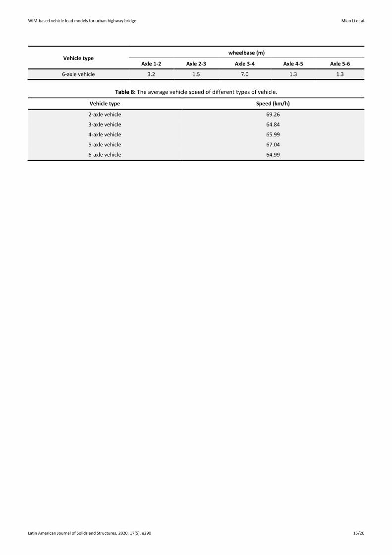
A finite element (FE) model for a 32 m simply supported box girder bridge is established by using the ANSYS software. The cross-section in the mid-span of the bridge is shown in Figure 12. According to the equivalent axle weight and the wheelbase, which are listed in Table 6 and Table 7, the vehicle load sare simplified as a set of concentrated forces and applied to the simply supported beam bridges. The representative wheelbase provided in “research on highway bridge vehicle load standard” is adopted as the equivalent wheelbase (Zhang, 2014). By using the moving load method, the bending moment responses at the mid-span of the 32m simply supported box girder bridge under different types are obtained and shown in Figure 13. In the calculation, the vehicle speeds are adopted using the in-site measurement data. The average vehicle speeds of different types of vehicle are shown in Table 8 and the calculation time interval is 0.01 s.

Figure 12: The mid-span cross-section of a 32m simply supported box girder bridge. (Units: cm)

Table 7: Wheelbase of vehicles.

Vehicle type wheelbase (m)

Axle 1-2 Axle 2-3 Axle 3-4 Axle 4-5 Axle 5-6

2-axle vehicle 5.0

3-axle vehicle 5.0 1.3

4-axle vehicle 2.5 6.0 1.3

5-axle vehicle 3.4 7.4 1.3 1.3



Vehicle type wheelbase (m)

Axle 1-2 Axle 2-3 Axle 3-4 Axle 4-5 Axle 5-6

6-axle vehicle 3.2 1.5 7.0 1.3 1.3

Table 8: The average vehicle speed of different types of vehicle.

Vehicle type Speed (km/h)

2-axle vehicle 69.26







Figure 13: The mid-span bending moment responses of a 32m simply supported box girder bridge under different types of vehicle.

Results indicate that the mid-span bending moment responses during the passing of vehicles have only a big cycle and some very small cycles, no matter how many axles the vehicle have. The maximum value of the moment is not generated when the vehicle reaches the mid-span, but is slightly delayed. In addition, for these simply supported beam bridges, when the axles pass, the shapes of bending moment curves are almost the same, but the values are different, which shows that the shape of the bending moment curve is not affected by the wheelbase and the axle weight distribution. Therefore, for this 32m simply supported box girder bridge, the number of fatigue stress cycles caused by each axle can be simplified to 1, and the maximum bending moment or stress amplitude can be calculated according to a set of concentrated forces acted on the most unfavorable position of the influence line.



6.2 Fatigue damage analysis of vehicles with different axles

Only considering the largest bending moment induced by the six-axle vehicles, the formula of the equivalent stress amplitude is,

1

eq1

k mm

i ii

S n S N

(25)

where Si is the magnitude of the stress amplitude decomposed by the rain flow counting method, ni is the number of the actual magnitude of the stress amplitude of Si, N is the total number of stress amplitude decomposed by rain flow counting method, m is a parameter determined by the S-N curve. For steel structures, m is normally taken as 3. The equivalent moment is calculated as follows,

1/33

D i riM f M (26)

where MD is the equivalent moment, and fi is the frequency where the moment Mri appears. In order to compare the contribution of each axle to structural fatigue damage, the damage ratio Dr is used. It indicates the cumulative damage caused by fatigue. The calculation formula is listed as follows,

i =m m

i i i ir m m

all all all all all

D n S n MD

D n S n M (27)

where Di is the cumulative damage caused by the vehicles with i axles, Dall is the cumulative damage caused by all vehicles, ni is the number of cycles caused by the vehicles with i axles, nall is the number of cycles caused by all vehicles, Si is the stress amplitude caused by the vehicles with i axles, Sall is the stress amplitude caused by all vehicles. Based on the rules of the AASSTO specification about the fatigue details, m = 3 is adopted.

The equivalent bending moment of the 32m simply supported box girder bridge and the damage ratio of vehicles with different axles are shown in Table 9. It should be noted that the composition of the vehicles listed in Table 9 is different with the ones in Table 1. The reason is that all vehicles below 30 kN are not considered for fatigue analysis. The proportion of vehicles with two axles in Table 9 is 29.78%, and the damage ratio to the bridge is not more than 10.91%. For vehicles with six axles, the proportion is 44.53% and the damage ratio is greater than 68.89%. It is seen that the six-axle vehicles are the main factor for the fatigue damage to the bridge. Therefore, the six-axle vehicle is adopted as the prototype of standard fatigue vehicle.

Table 9: The equivalent bending moment of the 32m simply supported box girder bridge and the damage ratio of vehicles with different axles.

Vehicle type Proportion

(%) Cycles

Amplitude of moment (kN·m)

Damage ratio (%)

2-axle vehicle 29.78 76155 61.06 10.91 3-axle vehicle 12.82 32798 109.53 8.43 4-axle vehicle 10.37 26523 148.49 9.24 5-axle vehicle 2.50 6383 169.12 2.53 6-axle vehicle 44.53 113893 257.81 68.89

6.3 The standard fatigue vehicle model

The prototype of standard fatigue vehicle is shown in Figure 14. If the GVW of this vehicle is W, then the axle weights are 0.12 W, 0.14 W, 0.2 W, 0.2 W, 0.17 W and 0.17 W, respectively. The wheelbases are 3.2 m, 1.5 m, 7.0 m, 1.3 m and 1.3 m, respectively.



Figure 14: The prototype of standard fatigue vehicle.

The equivalent weight of the standard fatigue vehicle can be calculated through the superposition of each axle weight by Equation (24).Based on the WIM data, the equivalent weight of the standard fatigue vehicle is 362.16 kN. Therefore, the axle weight has been allocated by using the ratio of the prototype of standard fatigue vehicle. For convenience, the equivalent weight and the axle weight has been slightly adjusted. Then the standard fatigue vehicle model for the small and medium span urban highway bridges located in Wuhan, China is proposed and shown in Figure 15.

Figure 15: The standard fatigue vehicle model for small and medium span urban highway bridges located in Wuhan.

7. Conclusions

In this study, the WIM data collected from the Wuhan Junshan Yangtze Bridge was used to analyze the traffic condition, gross vehicle weight, vehicle axle weight. The statistical models of GVW and vehicle load extreme value were developed. After that, the vehicle load extreme value in the design reference period was extrapolated and the fatigue vehicle load model was established. Results are listed as follows,

(1) The vehicle types of Junshan Yangtze River Bridge are mainly composed of two-axle vehicles and six-axle vehicles, among which two-axle vehicles account for 68.6% and six-axle vehicles account for 19.5%. GVW which is less than 100 kN accounts for 76.37%, fewer vehicles exceed 200 kN. Overloaded vehicles are mainly heavy vehicles among which 27.59% of six-axle vehicles are overloaded, both overloaded four-axle and five-axle vehicles are more than 10%. The maximum vehicle weight exceeds 1800 kN.

(2) The GVW of all vehicles presents multi-peak distribution. The triple Gaussian distribution is effective to fit the PDF of the GVW.

(3) GEV was used to fit the vehicle extreme value distribution for one month of measured WIM data. The extreme value of GVW of the bridge mainly distributed in the range of 400 kN to 1800 kN and the most concentrated distribution is at around 700 kN. Through extreme value estimation based on extreme value type I distribution, the maximum GVW in the design reference period (100 years) may be increased to 1922.2 kN.

(4) Based on the fatigue analysis of a 32 m simply supported box girder bridge, the six-axle vehicles are the main factor for the fatigue damage to the bridge. The six-axle vehicle is adopted as the prototype of standard fatigue vehicle and the fatigue vehicle model for the small and medium span urban highway bridges located in Wuhan, China is proposed.

Acknowledgements

The authors are grateful for the financial support from the Natural Science Foundation of China (Grant No. 51478472) and the Scientific Research Fund of Hunan Provincial Education Department (Project no. 19B106).

Author’s Contribuitions: Conceptualization, M Li and T Huang; Methodology, T Huang, J Liao and J Zhong; Investigation, M Li, T Huang, J Liao and J Zhong; Writing - original draft, M Li and J Liao; Writing - review & editing, T Huang; Funding acquisition, T Huang; Resources, T Huang and J Zhong; Supervision, T Huang and J Zhong.

Editor: Rogério José Marczak.



References

Cardini, A.J., Dewolf, J.T. (2009). Implementation of a Long-Term Bridge Weigh-In-Motion System for a Steel Girder Bridge in the Interstate Highway System. Journal of Bridge Engineering 14(6): 418-423.

Chen, B., Zhong, Z., Xie, X., Lu, P.Z. (2014). Measurement-based vehicle load model for urban expressway bridges. Mathematical Problems in Engineering 2014: 1-10.

Chotickai, P., Bowman, M.D. (2006). Truck Models for Improved Fatigue Life Predictions of Steel Bridges. Journal of Bridge Engineering 11(1): 71-80.

Cohen, H., Fu, G., Dekelbab, W., Moses, F. (2003). Predicting truck load spectra under weight limit changes and its application to steel bridge fatigue assessment. Journal of Bridge Engineering 8(5): 312-322.

Coles, S. (2001). An introduction to statistical modeling of extreme values, Springer Verlag (New York).

Croce, P., Salvatore, W. (2001). Stochastic Model for Multilane Traffic Effects on Bridges. Journal of Bridge Engineering 6(2): 136-143.

Feng, H.Y., Yin, T.H., Chen, B. (2015). Extreme estimation for vehicle load effect based on generalized Pareto distribution. Journal of Vibration and Shock 34(15): 7-11.

Fisher, J.W., Roy, S. (2011). Fatigue of steel bridge infrastructure. Structure and Infrastructure Engineering 7(7-8): 457-475.

Getachew, A., Obrien, E.J. (2007). Simplified site-specific traffic load models for bridge assessment. Structure and Infrastructure Engineering 3(4): 303-311.

Guo, T., Li, A., Zhao, D. (2008). Multiple-peaked probabilistic vehicle load model for highway bridge reliability assessment. Journal of Southeast University(Natural Science Edition) 38(5): 763-766.

Jacob, B.,Feypell-de La Beaumelle, V. (2010). Improving truck safety: Potential of weigh- in-motion technology. IATSS Research 34(1): 9-15.

Jacob, B., OBrien, E.J. (2005). Weigh-in-Motion: Recent developments in Europe. Proceedings of the 4th International Conference on WIM, ICWIM4, Taipei.

Kotz, S., Nadarajah, S. (2000). Extreme value distributions-theory and applications, Imperial College Press (London).

Laman, J.A., Nowak, A.S. (1996). Fatigue-Load Models for Girder Bridges. Journal of Structural Engineering 122(7): 726-733.

Lan, C.M., Li, H., Ou, J.P. (2011). Traffic load modelling based on structural health monitoring data. Structure and Infrastructure Engineering 7(5): 379-386.

Lu, N.W., Liu, Y., L., Deng, Y. (2019). Fatigue reliability evaluation of orthotropic steel bridge decks based on site-specific weigh-in-motion measurements. International Journal of Steel Structures 19 (1): 181-192.

Mckinnon, A.C. (2005). The economic and environmental benefits of increasing maximum truck weight: the british experience. Transportation Research Part D Transport & Environment 10(1): 77-95.

Mei, G., Qin, Q., Lin, D.-J. (2004). Bimodal renewal processes models of highway vehicle loads. Reliability Engineering and System Safety 83(3): 333-339.

Nowak, A.S. (1993). Live load model for highway bridges. Structural safety 13(1): 53-66.

Nowak, A.S., Hong, Y. (1991). Bridge live-load models. Journal of Structural Engineering 117(9): 2757-2767.

Nowak, A.S., Nassif, H., Defrain, L. (1993). Effect of truck loads on bridges. Journal of Transportation Engineering 119(6): 853-867.

Obrien, E.J., Enright, B. (2013). Using weigh-in-motion data to determine aggressiveness of traffic for bridge loading. Journal of Bridge Engineering 18(3): 232-239.

Obrien, E.J., Enright, B., Getachew, A. (2010). Importance of the tail in truck weight modeling for bridge assessment. Journal of Bridge Engineering 15(2): 210-213.

Obrien, E.J., Schmidt, F., Hajializadeh, D., Zhou, X.Y., Enright, B., Caprani, C.C., et al.(2015). A review of probabilistic methods of assessment of load effects in bridges. Structural Safety 53:44-56.



O’Connor, A., Eichinger, E.M. (2007). Site-specific traffic load modelling for bridge assessment. Proceedings of the Institution of Civil Engineers-Bridge Engineering 160(4): 185-194.

O’Connor, A., Obrien, E.J. (2005). Traffic load modelling and factors influencing the accuracy of predicted extremes. Canadian Journal of Civil Engineering 32(1): 270-278.

Robert, E. Melchers. (1999).Structural reliability analysis and prediction (2nd edition). New York: John Wiley & Sons.

Sivakumar, B., Ghosn, M. (2009). Collecting and using Weigh-in-Motion data in LRFD bridge design. Bridge Structures 5(4):151-158.

Worden, K., Cross, E.J. (2018). On switching response surface models, with applications to the structural health monitoring of bridges. Mechanical Systems & Signal Processing 98:139-156.

Zhao, H., Uddin, N., Shao, X.D., Zhu, P., Tan, C.J. (2015). Field-calibrated influence lines for improved axle weight identification with a bridge weigh-in-motion system. Structure and Infrastructure Engineering 11(6):721-743.

Zhao, J., Tabatabai, H. (2012). Evaluation of a permit vehicle model using weigh-in-motion truck records. Journal of Bridge Engineering 17(2): 389-392.

Zhao, S.J., Ren, W.X. (2017). Piecewise Truncation Probability Distribution Model of Vehicle Loads for Highway Bridges and Its Application. China Journal of Highway and Transport 30(06): 260-267.

Zhang, X.G. (2014). Research on highway bridge vehicle load standard, China Communications Press (Beijing).

wim-based vehicle load models for urban highway bridge

Documents