Wind Disturbance Rejection for an Insect-Scale Flapping-Wing Robot

Pakpong Chirarattananon1, Kevin Y. Ma2, Richard Cheng3, and Robert J. Wood2

Abstract— Despite having achieved unconstrained stableflight, the insect-scale flapping-wing robot is still tethered forpower and control. Towards the goal of operating a biologically-inspired robot autonomously outside of laboratory conditions.In this paper, we simulate outdoor disturbances in the lab-oratory setting and investigate the effects of wind gusts onthe flight dynamics of a millimeter-scale flapping wing robot.Simplified models describing the disturbance effects on therobot’s dynamics are proposed, together with two disturbancerejection schemes capable of estimating and compensating forthe disturbances. The proposed methods are experimentallyverified. The results show that they reduced the root meansquare position errors by approximately 50% when the robotwas subject to 60 cm·s−1 horizontal wind.

I. INTRODUCTION

Foreseeable applications of small flying robots in our ev-

eryday lives, ranging from city courier services to automated

aerial construction [1], have driven advances in research

in the area of Micro Aerial Vehicles (MAVs) as seen in

innumerable examples [1], [2], [3]. Among these, multi-

rotor vehicles have gained considerable popularity thanks

to simple mechanical designs and well-understood dynamic

properties.

Biologically-inspired MAVs are another platform for ac-

tive research [4], [5]. Flapping-wing devices are particularly

of interest owing to their expected maneuverability exem-

plified by their natural counterparts. Inspired by tiny flying

insects, researchers have developed and demonstrated stable

unconstrained flight of an insect-scale robot (shown in figure

1) in [6], [7]. The results reflect the culmination of research

in meso-scale actuation and manufacturing technology [6],

[8], as well as understanding in control, stability, and aero-

dynamics of flapping flight [9], [10], [11].

Despite having achieved stable flight, the flapping-wing

robot prototype in figure 1 is still tethered for power and

control. Limited by the payload capacity (the robot can

This work was partially supported by the National Science Foundation(award number CCF-0926148), and the Wyss Institute for BiologicallyInspired Engineering. Any opinions, findings, and conclusions or recom-mendations expressed in this material are those of the authors and do notnecessarily reflect the views of the National Science Foundation.

1Pakpong Chirarattananon is with the Department of Mechanical andBiomedical Engineering, City University of Hong Kong, Hong Kong (email:pakpong.c@cityu.edu.hk).

2Kevin Y. Ma and Robert J. Wood are with the School of Engineeringand Applied Sciences, Harvard University, Cambridge, MA 02138, USA,and the Wyss institute for Biologically Inspired Engineering, HarvardUniversity, Boston, MA, 02115, USA (email: kevinma@seas.harvard.edu;rjwood@eecs.harvard.edu).

3Richard Cheng is with the Department of Mechanical and AerospaceEngineering, Princeton University, Princeton, NJ 08544, USA (email: rc-three@princeton.edu).

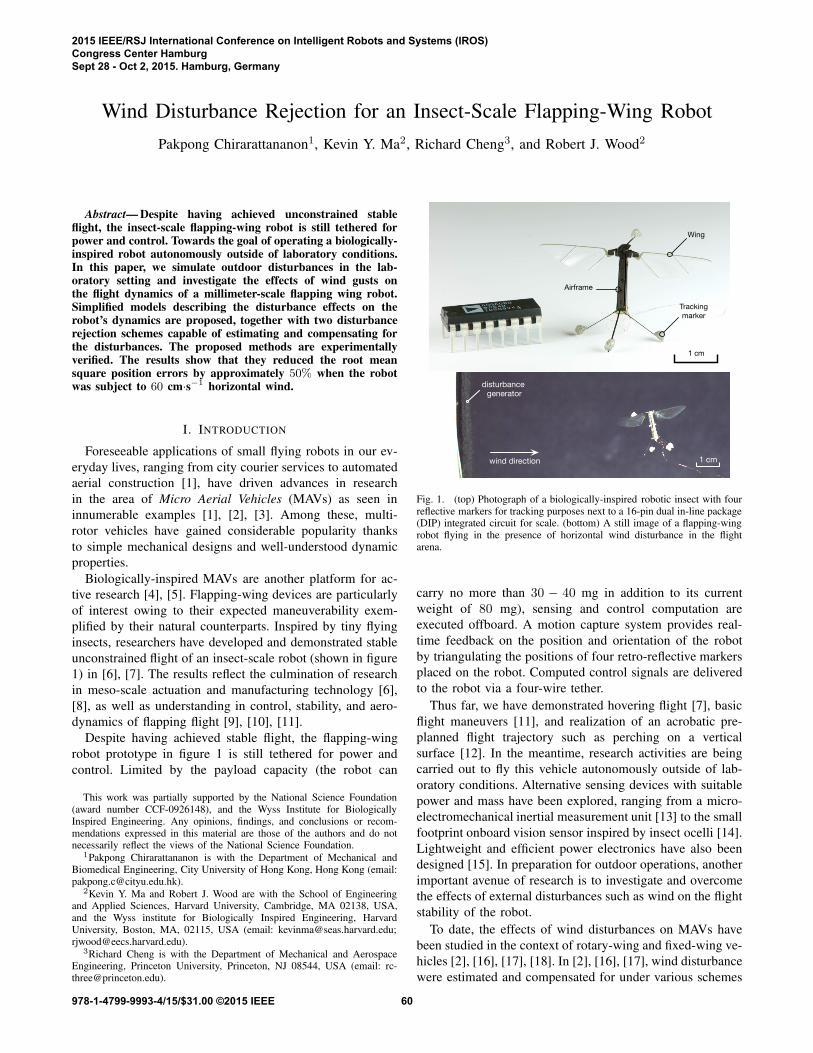
1 cm

Wing

Airframe

Tracking

marker

wind direction

disturbance generator

1 cm

Fig. 1. (top) Photograph of a biologically-inspired robotic insect with fourreflective markers for tracking purposes next to a 16-pin dual in-line package(DIP) integrated circuit for scale. (bottom) A still image of a flapping-wingrobot flying in the presence of horizontal wind disturbance in the flightarena.

carry no more than 30 − 40 mg in addition to its current

weight of 80 mg), sensing and control computation are

executed offboard. A motion capture system provides real-

time feedback on the position and orientation of the robot

by triangulating the positions of four retro-reflective markers

placed on the robot. Computed control signals are delivered

to the robot via a four-wire tether.

Thus far, we have demonstrated hovering flight [7], basic

flight maneuvers [11], and realization of an acrobatic pre-

planned flight trajectory such as perching on a vertical

surface [12]. In the meantime, research activities are being

carried out to fly this vehicle autonomously outside of lab-

oratory conditions. Alternative sensing devices with suitable

power and mass have been explored, ranging from a micro-

electromechanical inertial measurement unit [13] to the small

footprint onboard vision sensor inspired by insect ocelli [14].

Lightweight and efficient power electronics have also been

designed [15]. In preparation for outdoor operations, another

important avenue of research is to investigate and overcome

the effects of external disturbances such as wind on the flight

stability of the robot.

To date, the effects of wind disturbances on MAVs have

been studied in the context of rotary-wing and fixed-wing ve-

hicles [2], [16], [17], [18]. In [2], [16], [17], wind disturbance

were estimated and compensated for under various schemes

2015 IEEE/RSJ International Conference on Intelligent Robots and Systems (IROS)Congress Center HamburgSept 28 - Oct 2, 2015. Hamburg, Germany

978-1-4799-9993-4/15/$31.00 ©2015 IEEE 60

in the problem of position control of quadrotors. The pro-

posed methods were verified in simulations. Nevertheless, the

lack of experimental validation casts doubt on the accuracy

of the aerodynamic models and the effects of turbulence flow

on the vehicles. In another example [18], researchers tackle

the wind disturbance problem for a fixed-wing MAV in an at-

tempt to perch on a wire by experimentally characterizing the

wind profile and elegantly designing an adaptive controller

with verified regions of attraction. The strategies were then

successfully tested in an outdoor environment. The effects

of wind disturbances on flapping flight are different owing

to unsteady aerodynamics. The topic of disturbances and

forward flight has been mostly rudimentarily studied in real

insects [9], [10], [19]. In this work, we seek to stabilize and

control the position of an insect-scale flapping-wing robot

in the presence of wind gusts by rejecting the disturbances

based on simplified aerodynamic models.

First, we briefly cover the dynamic model of the robot.

Based on previous work and preliminary results, we propose

a simple model describing the effects of the wind distur-

bances on flight dynamics for flight control purposes. Two

disturbance rejection strategies compatible with the existing

flight controller and the proposed disturbance model are de-

scribed. The two schemes are employed in the flight control

experiments to stabilize the flapping-wing robot under the

presence of 60 cm·s−1 horizontal wind. Finally, experimental

results are presented and discussed.

II. MODELING OF ROBOT’S DYNAMICS AND THE

EFFECTS OF WIND DISTURBANCES

A. Robot Description and Dynamics

The flight-capable 80-mg flapping-wing robot in figure

1 was designed after its underactuated predecessor in [20].

The current prototype, with a wingspan of 3.5 cm, is fab-

ricated using laser micro-machining and the Smart Com-

posite Microstructures (SCM) process as detailed in [6].

Two piezoelectric bending actuators serve as flight muscles.

When a voltage is applied across the piezoelectric plates,

it induces approximately linear motion at the tip of the

actuator, which is transformed into an angular wing motion

by a spherical four-bar transmission. Each actuator is capable

of independently driving a single wing. It turns out that

mechanical properties of the coupled actuator-transmission-

wing subsystems approximate that of a second-order linear

system [21], roughly equivalent to an ideal forced mass-

spring-damper system. The elastic potential energy of the

bending actuator resembles the potential energy stored in a

spring, while energy dissipated through aerodynamic drag

on the wing parallels the loss in a damper. In operation,

the robot is nominally driven with signals near the system’s

resonant frequency of 120 Hz to maximize the flapping

stroke amplitude and minimize the reactive power expended

by wing inertia. Lift is modulated by altering the amplitudes

of the driving signals. Pitch, roll, and yaw torques are

generated by appropriately modifying the nominal sinusoidal

signals as described in [7]. The inherent instability of the

Driving

signals

Position and

orientation

feedback

Flight

controller

Inertial

frame

Body

frame

y

x

z

Y

X

Z

Center

of mass

Disturbance

generator

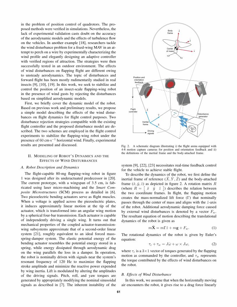
Fig. 2. A schematic diagram illustrating i) the flight arena equipped with4-8 motion capture cameras for position and orientation feedback and ii)the definitions of the inertial frame and the body-attached frame.

system [9], [22], [23] necessitates real-time feedback control

for the vehicle to achieve stable flight.

To describe the dynamics of the robot, we first define the

inertial frame of reference (X, Y , Z) and the body-attached

frame (x, y, z) as depicted in figure 2. A rotation matrix R(where R =

[

x y z]

) describes the relation between

the two coordinate frames. In flight, the flapping motion

creates the mass-normalized lift force (Γ) that nominally

passes through the center of mass and aligns with the z-axis

of the robot. Additional aerodynamic damping force caused

by external wind disturbances is denoted by a vector Fw.

The resultant equation of motion describing the translational

dynamics of the robot is given as

mX = mΓz +mg + Fw. (1)

The rotational dynamics of the robot is given by Euler’s

equation:

τc + τw = Jω + ω × Jω, (2)

where τc is a 3×1 vector of torques generated by the flapping

motion as commanded by the controller, and τw represents

the torque contributed by the effects of wind disturbances on

the robot.

B. Effects of Wind Disturbance

In this work, we assume that when the horizontally moving

air encounters the robot, it gives rise to a drag force linearly

61

proportional to relative velocity. The linear assumption, as

presented in [23], [10], is due to the dominant contribution

from the interaction between the flapping wings and mov-

ing air. Empirical evidence suggests that this assumption

is approximately valid for a flapping-wing robot at this

scale for both head-on wind and lateral wind at low wind

speed (less than 1.5 m·s−1) [23]. By a similar argument,

laterally moving air would also cause additional lift in the

direction perpendicular to the drag (or along the z-axis). As

a result, we propose that the effects of wind disturbance on

the translational dynamics of a flapping-wing robot can be

described as

Fw = mbx (v · x) x+mby (v · y) y +mbz ‖v × z‖ z, (3)

where v = [vx, vy, 0]T

is a vector of relative air velocity.

For a hovering or near-hovering robot, v may be taken as

the disturbance wind velocity. Equation (3) assumes different

normalized damping coefficients (bx,by, bz) for drag (and lift)

along different body axes. Wind-tunnel experiments in [23]

suggest that the values of bx and by are comparable. The

distinct structure of Fw along the z-direction is owing to

the mentioned lift, which is assumed to be a linear function

of wind velocity on the x − y plane. Since Fw does not

necessarily pass through the center of mass of the robot, it

is anticipated to perturb the rotational dynamics of the robot

as well. We model the torque contribution from the wind

disturbance on the robot as the following

τw = J[

−βx (v · y) βy (v · x) 0]T

, (4)

where βx and βy are corresponding rotational damping

coefficients (normalized by the inertia J). Equation (4) can

be interpreted as the the product of Fw with appropriate ef-

fective moment arms and normalizing factors. The absence of

torque along the z-axis is based on an assumption regarding

the symmetry of the robot and its nominal flapping motions.

It is important to mention that equations (3) and (4) are

modeled based on limited experimental evidence. While their

validity is debatable, the primary goal is that they capture

the dominant effects observed in the experiments and are

sufficiently accurate for controller design purposes.

III. CONTROL STRATEGIES

A. Adaptive Tracking Flight Controller

In this paper, we propose two wind disturbance rejection

schemes and demonstrate how they can be implemented

on the existing adaptive tracking flight controller, which

is presented in [24]. For completeness, in this section we

briefly describe the fundamental elements of the existing

flight controller. The explanation on how the disturbance

rejection components are integrated into the flight controller

is given in section III-B.

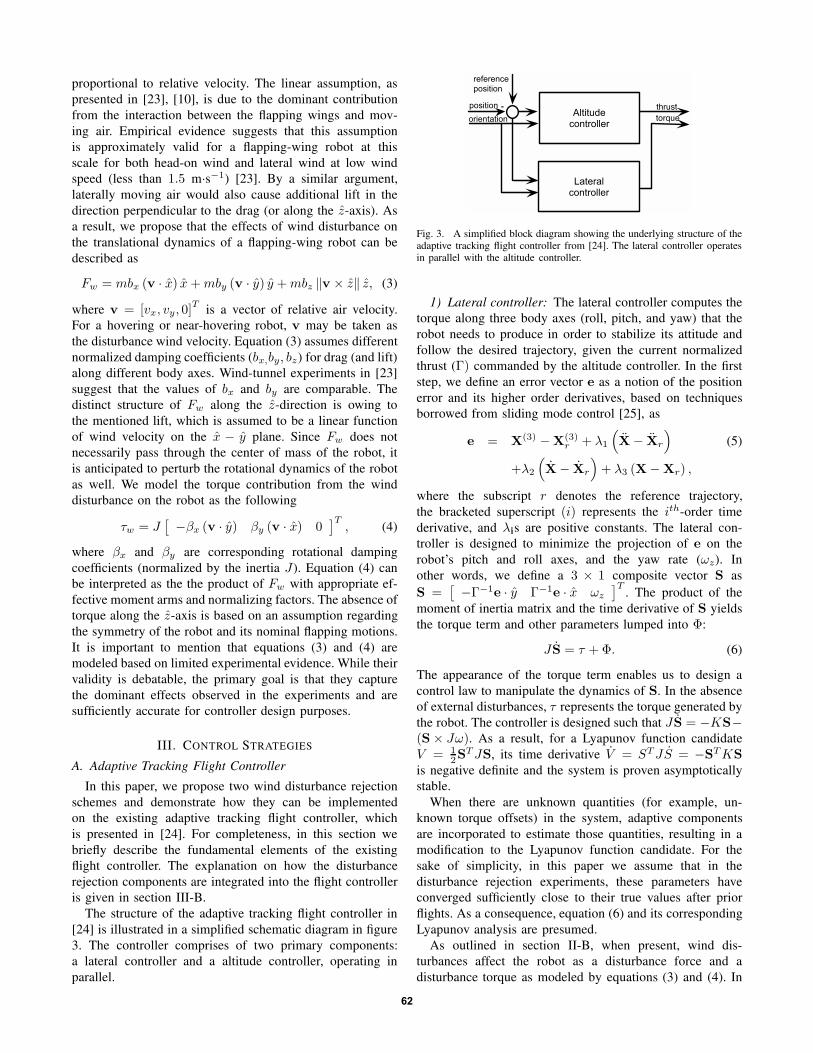
The structure of the adaptive tracking flight controller in

[24] is illustrated in a simplified schematic diagram in figure

3. The controller comprises of two primary components:

a lateral controller and a altitude controller, operating in

parallel.

Lateralcontroller

thrust

torqueAltitudecontroller

orientation

position -

reference

position

Fig. 3. A simplified block diagram showing the underlying structure of theadaptive tracking flight controller from [24]. The lateral controller operatesin parallel with the altitude controller.

1) Lateral controller: The lateral controller computes the

torque along three body axes (roll, pitch, and yaw) that the

robot needs to produce in order to stabilize its attitude and

follow the desired trajectory, given the current normalized

thrust (Γ) commanded by the altitude controller. In the first

step, we define an error vector e as a notion of the position

error and its higher order derivatives, based on techniques

borrowed from sliding mode control [25], as

e = X(3) −X(3)r + λ1

(

X− Xr

)

(5)

+λ2

(

X− Xr

)

+ λ3 (X−Xr) ,

where the subscript r denotes the reference trajectory,

the bracketed superscript (i) represents the ith-order time

derivative, and λis are positive constants. The lateral con-

troller is designed to minimize the projection of e on the

robot’s pitch and roll axes, and the yaw rate (ωz). In

other words, we define a 3 × 1 composite vector S as

S =[

−Γ−1e · y Γ−1e · x ωz

]T. The product of the

moment of inertia matrix and the time derivative of S yields

the torque term and other parameters lumped into Φ:

J S = τ +Φ. (6)

The appearance of the torque term enables us to design a

control law to manipulate the dynamics of S. In the absence

of external disturbances, τ represents the torque generated by

the robot. The controller is designed such that J S = −KS−(S× Jω). As a result, for a Lyapunov function candidate

V = 12S

TJS, its time derivative V = STJS = −STKS

is negative definite and the system is proven asymptotically

stable.

When there are unknown quantities (for example, un-

known torque offsets) in the system, adaptive components

are incorporated to estimate those quantities, resulting in a

modification to the Lyapunov function candidate. For the

sake of simplicity, in this paper we assume that in the

disturbance rejection experiments, these parameters have

converged sufficiently close to their true values after prior

flights. As a consequence, equation (6) and its corresponding

Lyapunov analysis are presumed.

As outlined in section II-B, when present, wind dis-

turbances affect the robot as a disturbance force and a

disturbance torque as modeled by equations (3) and (4). In

62

order to stabilize the robot and ensure that the trajectory

tracking ability is not compromised, we need to modify the

flight controller accordingly.

Fortunately, the derivation of the lateral flight controller

above (for the complete version, refer to [24]) does not

explicitly rely on the translational dynamics (equation (1)).1

The error vector e is minimized when the robot perfectly

follows the reference trajectory, independent of the existence

of the disturbance force. On the other hand, the torque

disturbance alters equation (6) by introducing the τw term.

This leaves the time derivative of the Lyapunov function as

V = −STKS + ST τw, which is no longer guaranteed to

be negative definite. This demands a disturbance rejection

component to stabilize the lateral dynamics as shown later

in section (III-B).

2) Altitude controller: While the altitude controller is

presented and executed separately from the lateral controller,

they operate in parallel and could be regarded as a single

block in the diagram in figure 3. Here the altitude controller

regulates altitude by controlling the thrust generated by

the robot. To inspect the altitude dynamics, we project the

translational dynamics from equation (1) along the Z-axis,

Z = X ·[

0 0 1]T

= ΓR33 − g + (Fw/m) ·[

0 0 1]T

. (7)

It follows that the projection of Fw on the Z-axis concerns

the following terms:

bx (v · x) x ·[

0 0 1]T

= −bxR13R33vx

by (v · y) y ·[

0 0 1]T

= −bxR23R33by

bz ‖v × z‖ z ·[

0 0 1]T

= bzR33 ‖v × z‖ . (8)

The first two terms involving bx and by can be positive

or negative, depending on the robot’s orientation and the

wind direction, whereas the last term is always positive

when the robot is in flight. Preliminary experimental results

indicate that lateral wind brings about a dramatic increase

in lift, suggesting that the last term dominates, allowing us

to neglect bx and by terms. The problem can be simplified

further by assuming the condition R13, R23 ≪ 1—that is,

the robot remains near the upright orientation,

(Fw/m) ·[

0 0 1]T

≈ bzR33

[

‖v‖2

− (vxR13 + vyR23)2]

1

2

≈ bzR33 ‖v‖+O(

ǫ2)

≈ bzR33 ‖v‖ , (9)

where ǫ ≈ R13, R23. When substituted back to equation (7),

this yields

z = (Γ + bz ‖v‖)R33 − g. (10)

For a constant or slowly time-varying wind disturbance, the

bz ‖v‖ term behaves identically to a constant offset to the

1This is true when the disturbance force is constant or slowly time-varyingin the inertial frame.

generated thrust. This property makes the disturbance effects

on the altitude dynamics easy to deal with by the current

adaptive controller.

B. Wind Disturbance Rejection Schemes

1) Adaptive estimation: One strategy to counteract wind

disturbances is to fully embrace the constant or slowly time-

varying wind assumption, and adaptively estimate this effect

based on feedback. We first consider the effect of the torque

disturbance on the lateral controller by expressing equation

(4), which involves four unknown parameters: namely βx,

βy , vx, and vy . While it is possible to adaptively estimate four

parameters, we opt to reduce the number to two by assuming

βx = βy = β. In this case, the damping coefficient β can be

lumped with the wind parameters vx and vy , allowing them

to be estimated together as

τw = J

−R12 −R22

R11 R21

0 0

[

βvxβvy

]

= JY a, (11)

where we have defined a 3×2 matrix Y and a 2×1 vector of

unknowns a accordingly. Let the notations (·) and (·) denote

an estimated quantity and the estimation error (i.e., a = a−a). In flight, we command the controller to compensate for

the torque disturbance by countering it with its estimate in

addition to the existing control law. The time derivative of

the composite variable S from section III-A.1 becomes

J S = −KS− (S× Jω) + JY a− JY a

= −KS− (S× Jω)− JY a. (12)

By re-defining the Lyapunov function candidate as V =12S

TJS+ 12 a

TΛ−1a for some positive diagonal gain matrix

Λ and employing the adaptive law ˙a = ΛY T JTS, it can be

shown that we recover the condition V = −STKS. That is,

stability is guaranteed in a Lyapunov sense.

A similar strategy could be implemented to cope with the

disturbance term in the altitude dynamics in equation (10).

Since the altitude controller, taken from [24], employed in

this work already possesses the ability to adaptively estimate

and compensate for constant thrust offsets, it benefits from

the fact that the effect of the constant wind disturbance

is identical to an unknown thrust offset. Essentially, we

do not need to explicitly amend the altitude controller to

tackle lateral wind, except for changing the adaptive gain to

be sufficiently large in order for the estimates to converge

quickly.

2) Least-squares estimation: While the adaptive estima-

tion method is simple and easy to implement, it relies heavily

on the assumption that the wind disturbance is constant

or slowly time-varying. Hence, we propose an alternative

approach that relaxes the constant assumption slightly, al-

lowing the adaptive algorithm to capture, to some extent,

the temporal structure of the wind disturbance. The proposed

strategy resembles the adaptive estimation method in that it

63

first estimates the disturbance and applies a counteracting

input to eliminate the effects from the disturbance.

To derive the LS estimator component for the lateral

controller, we begin with the partial result from equation

(12), but representing the JY a term by τw, such that J S =−KS − (S× Jω) + τw − τw. Here the controller applies

the compensating torque τw based on the current estimate

of τw. This equation can be re-arranged and applied a first-

order low pass filter fp = p/ (s+ p), where s is a Laplace

variable and p−1 is an associated time constant,

fp

{

J S−KS+ (S× Jω) + τw

}

= fp {τw} . (13)

Denote the quantity on the left hand side of equation (13),

which is readily computable, as Ψ(t). The right hand side

of equation (13) can also be represented in the discrete-time

domain,

fp {τw} =1− e−pT

1− z−1e−pTz−1τw, (14)

where T is a discrete sampling time and z−1 denotes the

delay operator. Combining equations (13) and (14), we obtain

τ [ti−1] =1

1− e−pT

(

Ψ [ti]− e−pTΨ [ti−1])

, (15)

where [ti] is an index for the discrete time domain (i.e.,

ti − ti−1 = T ). The lumped estimates of wind parameters

can be found by representing τ as JY a, similar to equation

(11) as

a [ti−1] =Y −1 [ti−1] J

−1

1− e−pT

(

Ψ [ti]− e−pTΨ [ti−1])

. (16)

To obtain the estimate of a, we assumes that a may pos-

sess some temporal structure. This inspires us to estimate

a via a finite impulse response (FIR) filter as a[ti] =∑N

k=1 σkz−kna [ti]. Here, N is the filter length, k can

be regarded as an arbitrary step size, and σks are cor-

responding coefficients to be found. Then the algorithm

for a standard least-squares estimator with an exponential

forgetting factor (γ) is used to determine σs that minimize´ t

δe−γ(t−δ) ‖a (s)− a (s)‖

2dδ [25]. The current estimate

a(t) depends entirely on these σ’s and a’s in the past. Since,

this is an iterative algorithm, σ′s are updated every time step.

The controller then compensates for the torque disturbances

by projecting a back to the appropriate space as τw = JY a.

The same strategy applies to the altitude controller in an

attempt to correct for the disturbance force on the altitude

dynamics. To elaborate, the unknown offset bz ‖v‖ is treated

as a single parameter using the FIR filter. That is, it may be

written as a combination of its past values in the same way

that a is estimated. In this case the least-square method is

implemented without the need for projection. The complete

derivation is omitted for brevity.

IV. EXPERIMENTAL RESULTS

A. Experimental Setup

Unconstrained flight experiments were performed in a

flight arena equipped with 4-8 motion capture VICON cam-

eras. They provide position and orientation feedback of the

robot at the rate of 500 Hz, covering a tracking volume of

0.3 × 0.3 × 0.3 m. Control algorithms were implemented

on an xPC Target (MathWorks) environment and executed at

the rate of 10 kHz for both input sampling and output signal

generation. Signals are generated through a digital-to-analog

converter, amplified, and then delivered to the robot through

four 51-gauge copper wires.

Prior to the disturbance rejection experiments, the robots

underwent an extensive characterization and trimming pro-

cess. This started by a visual inspection of the wings’

kinematics at various operating frequencies to identity the

system’s resonance frequency, symmetry, and flapping ampli-

tudes. Open-loop trimming flights were performed to deter-

mine suitable driving signals or the trimmed conditions that

allowed the robot to liftoff, ideally vertically, in short (<0.3

seconds) flights. With closed-loop feedback, a well-trimmed

robot could stabilize in short hovering flights (5-10 seconds)

which served as closed-loop trimming flights. In these flights,

the adaptive algorithms continuously updated the estimates

of the unknown parameters. Once they converged, the insect-

scale robot was able to hover at a designated setpoint

within a body length. In case of mechanical fatigue or any

damages on the robot, which occurs regularly (the lifetime

of flexure-based wing hinges, for example, are <10 minutes

[26]), manual part replacements or repairs are sometimes

possible. In such circumstances, the complete characterizing

and trimming process has to be repeated.

B. Wind Disturbance Generator

We constructed a low-speed wind disturbance generator

from an array of nine 12V DC fans fitted in a 15× 15× 20cm box, capable of creating wind disturbances in a horizontal

plane. An Arduino combined with an amplification circuit

were used to execute commands received from the xPC

Target system. In steady state, the wind generator is able

to consistently generate wind with the speed ranging from

(20−100)±2 cm·s−1 as verified by a hot-wire anemometer.

The variation of the wind speed over the area of 15× 15 cm

around the setpoint (at the setpoint height) is generally less

than ±3 cm·s−1.

C. Flight Experiments with Constant Wind Disturbances

To investigate the effects of lateral wind disturbances on

the flapping-wing robotic insect, we carried out a series

of experiments with the disturbance generator programmed

to produce constant 60 cm·s−1 wind in steady state. The

wind blew in the positive X direction. In the first set of

experiments (four flights), no disturbance rejection scheme

was implemented. Then seven flights (three and four) were

performed with the adaptive estimation scheme and the least-

squares estimator. Lastly both schemes were tested together

in three flights. In summary, four sets of experiments were

performed.

The time-trajectory plots of all 14 flights are shown in

figure 4(a), together with the averaged wind profile at the

setpoints measured by a hot-wire anemometer from six trials.

64

060

win

d s

peed (

cm

/s)

0 7time (s)

no compensation 5.36

adaptive 3.40

least−squares 2.25

adaptive+LS 2.40

0 6RMS position error (cm)

(a)

(b)

no compensation (4 flights)

18

X p

ositio

n (

cm

)0

018

Z p

ositio

n (

cm

)

adaptive (3 flights)

18

X p

ositio

n (

cm

)0

018

Z p

ositio

n (

cm

)

least−squares (4 flights)

18

X p

ositio

n (

cm

)0

018

Z p

ositio

n (

cm

)

18

adaptive+LS (3 flights)

X p

ositio

n (

cm

)0

0 7time (s)

018

Z p

ositio

n (

cm

)

0 7time (s)

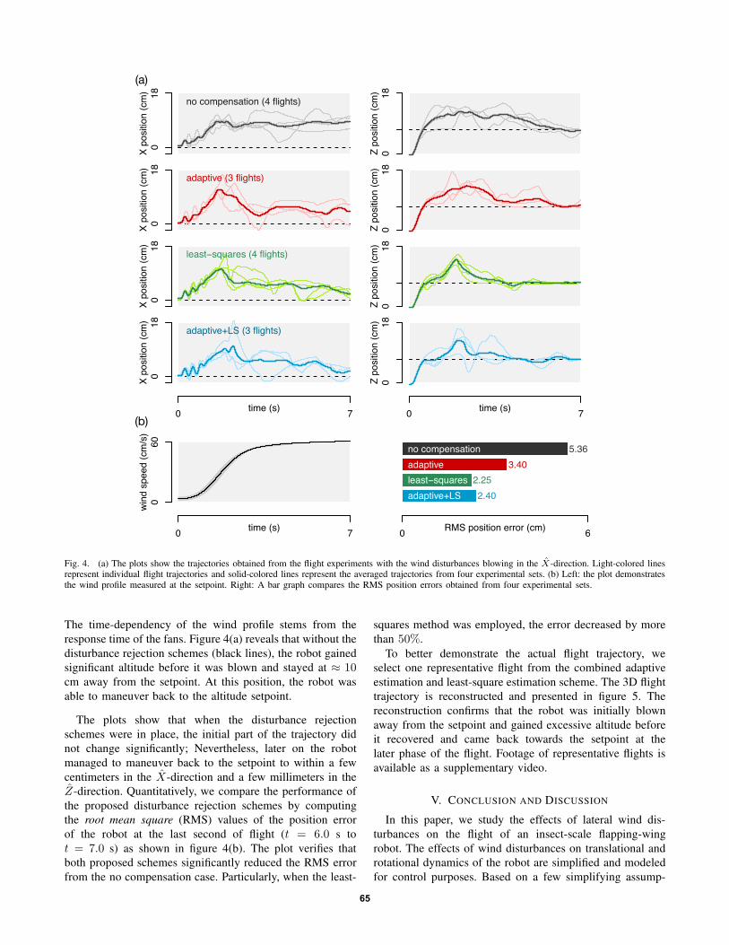
Fig. 4. (a) The plots show the trajectories obtained from the flight experiments with the wind disturbances blowing in the X-direction. Light-colored linesrepresent individual flight trajectories and solid-colored lines represent the averaged trajectories from four experimental sets. (b) Left: the plot demonstratesthe wind profile measured at the setpoint. Right: A bar graph compares the RMS position errors obtained from four experimental sets.

The time-dependency of the wind profile stems from the

response time of the fans. Figure 4(a) reveals that without the

disturbance rejection schemes (black lines), the robot gained

significant altitude before it was blown and stayed at ≈ 10cm away from the setpoint. At this position, the robot was

able to maneuver back to the altitude setpoint.

The plots show that when the disturbance rejection

schemes were in place, the initial part of the trajectory did

not change significantly; Nevertheless, later on the robot

managed to maneuver back to the setpoint to within a few

centimeters in the X-direction and a few millimeters in the

Z-direction. Quantitatively, we compare the performance of

the proposed disturbance rejection schemes by computing

the root mean square (RMS) values of the position error

of the robot at the last second of flight (t = 6.0 s to

t = 7.0 s) as shown in figure 4(b). The plot verifies that

both proposed schemes significantly reduced the RMS error

from the no compensation case. Particularly, when the least-

squares method was employed, the error decreased by more

than 50%.

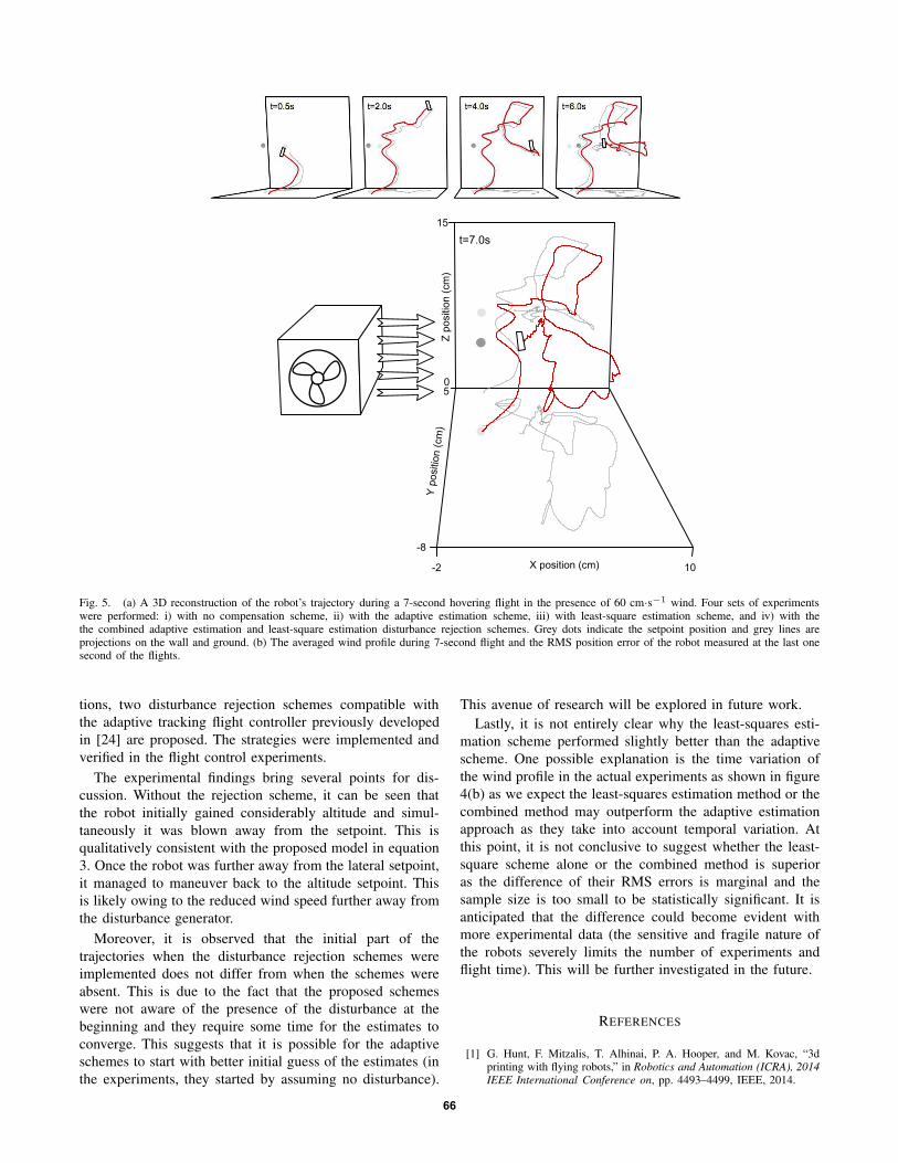
To better demonstrate the actual flight trajectory, we

select one representative flight from the combined adaptive

estimation and least-square estimation scheme. The 3D flight

trajectory is reconstructed and presented in figure 5. The

reconstruction confirms that the robot was initially blown

away from the setpoint and gained excessive altitude before

it recovered and came back towards the setpoint at the

later phase of the flight. Footage of representative flights is

available as a supplementary video.

V. CONCLUSION AND DISCUSSION

In this paper, we study the effects of lateral wind dis-

turbances on the flight of an insect-scale flapping-wing

robot. The effects of wind disturbances on translational and

rotational dynamics of the robot are simplified and modeled

for control purposes. Based on a few simplifying assump-

65

t=0.5s t=2.0s t=4.0s t=6.0s

t=7.0s

-2 10

-8

50

15

X position (cm)

Y p

ositio

n (

cm

)Z

po

sitio

n (

cm

)

Fig. 5. (a) A 3D reconstruction of the robot’s trajectory during a 7-second hovering flight in the presence of 60 cm·s−1 wind. Four sets of experimentswere performed: i) with no compensation scheme, ii) with the adaptive estimation scheme, iii) with least-square estimation scheme, and iv) with thethe combined adaptive estimation and least-square estimation disturbance rejection schemes. Grey dots indicate the setpoint position and grey lines areprojections on the wall and ground. (b) The averaged wind profile during 7-second flight and the RMS position error of the robot measured at the last onesecond of the flights.

tions, two disturbance rejection schemes compatible with

the adaptive tracking flight controller previously developed

in [24] are proposed. The strategies were implemented and

verified in the flight control experiments.

The experimental findings bring several points for dis-

cussion. Without the rejection scheme, it can be seen that

the robot initially gained considerably altitude and simul-

taneously it was blown away from the setpoint. This is

qualitatively consistent with the proposed model in equation

3. Once the robot was further away from the lateral setpoint,

it managed to maneuver back to the altitude setpoint. This

is likely owing to the reduced wind speed further away from

the disturbance generator.

Moreover, it is observed that the initial part of the

trajectories when the disturbance rejection schemes were

implemented does not differ from when the schemes were

absent. This is due to the fact that the proposed schemes

were not aware of the presence of the disturbance at the

beginning and they require some time for the estimates to

converge. This suggests that it is possible for the adaptive

schemes to start with better initial guess of the estimates (in

the experiments, they started by assuming no disturbance).

This avenue of research will be explored in future work.

Lastly, it is not entirely clear why the least-squares esti-

mation scheme performed slightly better than the adaptive

scheme. One possible explanation is the time variation of

the wind profile in the actual experiments as shown in figure

4(b) as we expect the least-squares estimation method or the

combined method may outperform the adaptive estimation

approach as they take into account temporal variation. At

this point, it is not conclusive to suggest whether the least-

square scheme alone or the combined method is superior

as the difference of their RMS errors is marginal and the

sample size is too small to be statistically significant. It is

anticipated that the difference could become evident with

more experimental data (the sensitive and fragile nature of

the robots severely limits the number of experiments and

flight time). This will be further investigated in the future.

REFERENCES

[1] G. Hunt, F. Mitzalis, T. Alhinai, P. A. Hooper, and M. Kovac, “3dprinting with flying robots,” in Robotics and Automation (ICRA), 2014

IEEE International Conference on, pp. 4493–4499, IEEE, 2014.

66

[2] A. Mokhtari and A. Benallegue, “Dynamic feedback controller of eulerangles and wind parameters estimation for a quadrotor unmannedaerial vehicle,” in Robotics and Automation, 2004. Proceedings.

ICRA’04. 2004 IEEE International Conference on, vol. 3, pp. 2359–2366, IEEE, 2004.

[3] F. Bourgeois, L. Kneip, S. Weiss, and R. Siegwart, “Delay and dropouttolerant state estimation for mavs,” in Experimental Robotics, pp. 571–584, Springer, 2014.

[4] L. Daler, S. Mintchev, C. Stefanini, and D. Floreano, “A bioinspiredmulti-modal flying and walking robot,” Bioinspiration & biomimetics,vol. 10, no. 1, p. 016005, 2015.

[5] J. Gerdes, A. Holness, A. Perez-Rosado, L. Roberts, A. Greisinger,E. Barnett, J. Kempny, D. Lingam, C.-H. Yeh, H. A. Bruck, et al.,“Robo raven: A flapping-wing air vehicle with highly compliant andindependently controlled wings,” Soft Robotics, vol. 1, no. 4, pp. 275–288, 2014.

[6] K. Y. Ma, S. M. Felton, and R. J. Wood, “Design, fabrication, andmodeling of the split actuator microrobotic bee,” in Intelligent Robots

and Systems (IROS), 2012 IEEE/RSJ International Conference on,pp. 1133–1140, IEEE, 2012.

[7] K. Y. Ma, P. Chirarattananon, S. B. Fuller, and R. J. Wood, “Controlledflight of a biologically inspired, insect-scale robot,” Science, vol. 340,no. 6132, pp. 603–607, 2013.

[8] J. Gafford, S. Kesner, R. Wood, and C. Walsh, “Microsurgical devicesby pop-up book mems,” ASME Paper No. DETC2013-13086, 2013.

[9] I. Faruque and J. S. Humbert, “Dipteran insect flight dynamics. part1 longitudinal motion about hover,” Journal of Theoretical Biology,vol. 264, no. 2, pp. 538–552, 2010.

[10] L. Ristroph, A. J. Bergou, J. Guckenheimer, Z. J. Wang, and I. Cohen,“Paddling mode of forward flight in insects,” Physical Review Letters,vol. 106, no. 17, p. 178103, 2011.

[11] P. Chirarattananon, K. Y. Ma, and R. J. Wood, “Adaptive control of amillimeter-scale flapping-wing robot,” Bioinspiration & Biomimetics,vol. 9, no. 2, p. 025004, 2014.

[12] P. Chirarattananon, K. Y. Ma, and R. J. Wood, “Fly on the wall,”in Biomedical Robotics and Biomechatronics (2014 5th IEEE RAS &

EMBS International Conference on, pp. 1001–1008, IEEE, 2014.

[13] S. B. Fuller, E. F. Helbling, P. Chirarattananon, and R. J. Wood, “Usinga MEMS gyroscope to stabilize the attitude of a fly-sized hoveringrobot,” in IMAV 2014: International Micro Air Vehicle Conference

and Competition 2014, Delft, The Netherlands, August 12-15, 2014,Delft University of Technology, 2014.

[14] S. B. Fuller, M. Karpelson, A. Censi, K. Y. Ma, and R. J. Wood,“Controlling free flight of a robotic fly using an onboard vision sensorinspired by insect ocelli,” Journal of The Royal Society Interface,vol. 11, no. 97, p. 20140281, 2014.

[15] M. Lok, D. Brooks, R. Wood, and G.-Y. Wei, “Design and analysis ofan integrated driver for piezoelectric actuators,” in Energy ConversionCongress and Exposition (ECCE), 2013 IEEE, pp. 2684–2691, IEEE,2013.

[16] S. L. Waslander and C. Wang, “Wind disturbance estimation andrejection for quadrotor position control,” in AIAA Infotech@ Aerospace

Conference and AIAA Unmanned... Unlimited Conference, Seattle, WA,2009.

[17] J. Escareño, S. Salazar, H. Romero, and R. Lozano, “Trajectory controlof a quadrotor subject to 2D wind disturbances,” Journal of Intelligent& Robotic Systems, vol. 70, no. 1-4, pp. 51–63, 2013.

[18] J. L. Moore, Robust post-stall perching with a fixed-wing UAV. PhDthesis, Massachusetts Institute of Technology, 2014.

[19] S. B. Fuller, A. D. Straw, M. Y. Peek, R. M. Murray, and M. H.Dickinson, “Flying drosophila stabilize their vision-based velocitycontroller by sensing wind with their antennae,” Proceedings of the

National Academy of Sciences, vol. 111, no. 13, pp. E1182–E1191,2014.

[20] N. O. Pérez-Arancibia, K. Y. Ma, K. C. Galloway, J. D. Greenberg, andR. J. Wood, “First controlled vertical flight of a biologically inspiredmicrorobot,” Bioinspiration & Biomimetics, vol. 6, no. 3, p. 036009,2011.

[21] B. M. Finio, N. O. Pérez-Arancibia, and R. J. Wood, “Systemidentification and linear time-invariant modeling of an insect-sizedflapping-wing micro air vehicle,” in Intelligent Robots and Systems(IROS), 2011 IEEE/RSJ International Conference on, pp. 1107–1114,IEEE, 2011.

[22] N. Gao, H. Aono, and H. Liu, “Perturbation analysis of 6DoF flightdynamics and passive dynamic stability of hovering fruit fly drosophila

melanogaster,” Journal of theoretical biology, vol. 270, no. 1, pp. 98–111, 2011.

[23] S. B. Fuller, Z. E. Tech, P. Chirarattananon, N. O. Pérez-Arancibia,J. Greenberg, and R. J. Wood, “Stabilizing air dampers for insect-scalehovering aerial robots: An analysis of nonlinear dynamics based onflight tests gives design guidelines,” 2015. under review.

[24] P. Chirarattananon, K. Y. Ma, and R. J. Wood, “Single-loop control andtrajectory following of a flapping-wing microrobot,” in Robotics andAutomation (ICRA), 2014 IEEE International Conference on, pp. 37–44, IEEE, 2014.

[25] J.-J. E. Slotine, W. Li, et al., Applied nonlinear control, vol. 60.Prentice-Hall Englewood Cliffs, NJ, 1991.

[26] R. Malka, A. L. Desbiens, Y. Chen, and R. J. Wood, “Principles ofmicroscale flexure hinge design for enhanced endurance,” in Intelli-

gent Robots and Systems (IROS 2014), 2014 IEEE/RSJ InternationalConference on, pp. 2879–2885, IEEE, 2014.

67