wind energy facilities and residential properties: the

J R E R � V o l . 3 3 � N o . 3 – 2 0 1 1

W i n d E n e r g y F a c i l i t i e s a n d R e s i d e n t i a lP r o p e r t i e s : T h e E f f e c t o f P r o x i m i t y a n dV i e w o n S a l e s P r i c e s

A u t h o r s Ben Hoen, Ryan Wiser, Peter Cappers ,

Mark Thayer, and Gautam Sethi

A b s t r a c t This paper received a manuscript prize award for the bestresearch paper on Sustainable Real Estate (sponsored by theNAIOP Research Foundation) presented at the 2010 ARESAnnual Meeting.

Increasing numbers of communities are considering wind powerdevelopments. One concern within these communities is thatproximate property values may be adversely affected, yet therehas been little research on the subject. The present researchinvestigates roughly 7,500 sales of single-family homessurrounding 24 existing wind facilities in the United States.Across four different hedonic models, and a variety of robustnesstests, the results are consistent: neither the view of the windfacilities nor the distance of the home to those facilities is foundto have a statistically significant effect on sales prices, yet furtherresearch is warranted.

Wind power development has expanded dramatically in recent years (WEC, 2010)and that expansion is expected to continue (Global Wind Energy Council, 2008;Wiser and Hand, 2010). The U.S. Department of Energy, for example, publisheda report that analyzed the feasibility of meeting 20% of electricity demand in theUnited States with wind energy by 2030 (U.S. DOE, 2008).

Approximately 3,000 wind facilities would need to be sited, permitted, andconstructed to achieve a 20% wind electricity target in the U.S.1 Although surveysshow that public acceptance is high in general for wind energy (e.g., Firestoneand Kempton, 2006), a variety of local concerns exist that can impact the lengthand outcome of the siting and permitting process. One such concern is related tothe views of and proximity to wind facilities and how these might impactsurrounding property values. Surveys of local communities considering windfacilities have frequently found that adverse impacts on aesthetics and propertyvalues are in the top tier of concerns relative to other matters such as impacts onwildlife habitat and mortality, radar and communications systems, ground

2 8 0 � H o e n , W i s e r , C a p p e r s , T h a y e r , a n d S e t h i

transportation, and historic and cultural resources (e.g., BBC Research &Consulting, 2005; Firestone and Kempton, 2006).

Concerns about the possible impacts of wind facilities on residential propertyvalues can be categorized into three potential effects:

� Scenic Vista Stigma: A perception that a home may be devalued becauseof the view of a wind energy facility, and the potential impact of thatview on an otherwise scenic vista.

� Area Stigma: A perception that the general area surrounding a windenergy facility will appear more developed, which may adversely affecthome values in the local community regardless of whether any individualhome has a view of the wind turbines.

� Nuisance Stigma: A perception that factors that may occur in closeproximity to wind turbines, such as sound and shadow flicker, will havean adverse influence on home values.

Any combination of these three potential stigmas might affect a particular home.Consequently, each of the three potential impacts must be considered whenanalyzing the effects of wind facilities on residential sales prices.

This paper uses several hedonic pricing models to analyze a sample of 7,459 arms-length residential real estate transactions occurring between 1996 and 2007 forhomes located near 24 existing wind facilities spread across nine U.S. states. Inso doing, the paper investigates the degree to which views of and proximity towind facilities affect sales prices.

The remainder of the paper is organized as follows. The next section contains asummary of the existing literature that has investigated the effects of wind energyon residential property values. Then the data used in the analysis are described.Following that, a set of four hedonic models are described and estimated to testfor the existence of property value impacts associated with the wind energyfacilities. The findings regarding the existence and magnitude of the three stigmasmentioned above are described, as are a series of robustness tests intended toassess the reliability of the model results. The paper ends with a brief discussionof future research possibilities.

� P r e v i o u s R e s e a r c h

A variety of methods, including surveys of homeowners and real estate experts,simple analysis of sales transactions (e.g., t-test), and sophisticated empiricalanalysis of sales transactions (e.g., multiple regression), have been used to explorethe relationship between residential property values and views of and proximityto wind facilities. One of the overall conclusions that can be drawn from thisliterature is that wind facilities are often predicted to negatively impact residentialproperty values in pre-construction surveys (Haughton, Giuffre, Barrett, and

W i n d E n e r g y F a c i l i t i e s & R e s i d e n t i a l P r o p e r t i e s � 2 8 1

J R E R � V o l . 3 3 � N o . 3 – 2 0 1 1

Tuerck, 2004; Khatri, 2004; Firestone, Kempton, and Krueger, 2007; Kielisch,2009), but negative impacts have largely failed to materialize post-constructionwhen actual transaction data become available for analysis (Jerabek, 2001;Sterzinger, Beck, and Kostiuk, 2003; Hoen, 2006; Poletti, 2007; Sims, Dent, andOskrochi, 2008). In the only study using transaction data that did find astatistically significant adverse effect, the authors contend that the result was likelydriven by variables omitted from their analysis, and not by the presence of windfacilities (Sims and Dent, 2007). Other studies that have relied on market datahave sometimes found the possibility of negative effects, but the statisticalsignificance of those results has not been reported (e.g., Kielisch, 2009).

Potentially more important, the existing literature leaves much to be desired. First,many of the studies have relied only on surveys of homeowners or real estateprofessionals, rather than trying to quantify impacts based on market data (e.g.,Haughton, Giuffre, Barrett, and Tuerck, 2004; Goldman, 2006). Second, a numberof the studies that used market data conducted rather simplified analyses of thosedata, potentially not controlling for the many drivers (e.g., size and/or conditionof the home and lot size) of residential sales prices (e.g., Sterzinger, Beck, andKostiuk, 2003; McCann, 2008; Kielisch, 2009). Third, many of the studies haverelied upon a very limited number of residential sales transactions, and thereforemay not have had an adequate sample to statistically discern any property valueeffects, even if effects did exist (e.g., Jerabek, 2001). Fourth, and perhaps as aresult, many of the studies did not conduct, or at least have not published, thestatistical significance of their results. Fifth, when analyzed, there has been someemphasis on area stigma, and none of the studies has simultaneously investigatedall three possible stigmas listed above. Sixth, only a few of the studies (Hoen,2006; Sims and Dent, 2007; Sims, Dent, and Oskrochi, 2008; Kielisch, 2009)conducted field visits to the homes to assess the quality of the scenic vista fromthe home, and the degree to which the wind facility might impact that scenic vista.Finally, with two exceptions (Sims and Dent, 2007; Sims, Dent, and Oskrochi,2008), none of the studies were peer-reviewed in the academic literature.

� D a t a O v e r v i e w

The methods applied in the present work are intended to overcome many of thelimitations of the existing literature. First, a large amount of residential real estatetransaction data was collected from within ten miles of 24 different existing windfacilities in the U.S., allowing for a robust statistical analysis across a pooleddataset that includes a diverse group of wind facility sites. Second, all threepotential stigmas were investigated by exploring the potential impact of windfacilities on home values based both on the distance to and view of the facilitiesfrom the homes. Third, field visits were made to every home in the sample,allowing for a reliable assessment of the scenic vista enjoyed by each home andthe degree to which the wind facility was visible from the home, and to collectother value-influencing data from the field (e.g., if the home is situated on a cul-


Exhibi t 1 � Summary of Study Areas

StudyAreaCode Study Area Counties, States Facility Names

# ofTurbines

# ofMW

Max HubHeight(meters)

WAOR Benton and Walla WallaCounties, WA and UmatillaCounty, OR

Vansycle Ridge,Stateline, NineCanyon I & II,Combine Hills

582 429 60

TXHC Howard County, TX Big Spring I & II 46 34 80

OKCC Custer County, OK Weatherford I & II 98 147 80

IABV Buena Vista County, IA Storm Lake I & II,Waverly, Intrepid I& II

381 370 65

ILLC Lee County, IL Mendota Hills,GSG Wind

103 130 78

WIKCDC Kewaunee and DoorCounties, WI

Red River, Lincoln 31 20 65

PASC Somerset County, PA Green Mountain,Somerset,Meyersdale

34 49 80

PAWC Wayne County, PA Waymart 43 65 65

NYMCOC Madison and OneidaCounties, NY

Madison 7 12 67

NYMC Madison County, NY Fenner 20 30 66

Total 1,345 1,286

Notes: The ten study areas are located in nine separate states, and total 1,286 MW, or roughly13% of total U.S. wind power capacity installed as of the end of 2005. The 24 wind facilities arecomprised of 1,345 turbines, which have hub heights that range from a minimum of 50 meters toa maximum of 80 meters.

de-sac). Finally, a set of robustness tests, including the estimation of a number ofdifferent hedonic regression models, were conducted.

The 24 wind facilities included in the sample (Exhibits 1 and 2) were chosen froma set of 241 wind facilities in the U.S. with a nameplate capacity greater than 0.6megawatts (MW) and that were constructed prior to 2006.2 These facilities,encompassing 10 different study areas, were selected based on: (1) the number ofavailable residential real estate transactions both before and, more importantly,after wind facility construction, and especially in close proximity (e.g., within twomiles) to the facility; (2) the availability of comprehensive data on homecharacteristics, sales prices, and locations in electronic form from local assessors;


J R E R � V o l . 3 3 � N o . 3 – 2 0 1 1

Exhibi t 2 � Map of Study Areas and Potential Study Areas

The 24 wind facilities, selected from 241 potential facilities, were included in the sample, and encompassed 10different study areas.

and (3) the representativeness of the types of wind energy facilities being installedin the U.S.

As indicated in Exhibit 1, the ten study areas are located in nine separate states,include facilities in the Pacific Northwest, upper Midwest, the Northeast, and theSouth Central region, and total 1,286 MW, or roughly 13% of total U.S. windpower capacity installed at the time (the end of 2005). Turbine hub heights in thesample range from a minimum of 50 meters in the Washington/Oregon (WAOR)study area, to a maximum of 80 meters (TXHC, OKCC, and PASC), with nineof the ten study areas having maximum hub heights of at least 65 meters. Thesites include a diverse variety of land types, including combinations of ridgeline(WAOR, PASC, and PAWC), rolling hills (ILLC, WIKCDC, NYMCOC, andNYMC), mesa (TXHC), and windswept plains (OKCC and IABV).

Three primary sets of data are used in the analysis: tabular data, geographicinformation system (GIS) data, and field data, each of which is discussed below.Special attention is given to the field data collection process for the two qualitativevariables, both of which are essential to the analysis that follows: scenic vista andviews of turbines.

Tabular sales transaction data were obtained from assessors in the participatingcounties, and total 7,459 ‘‘valid’’3 transactions of single-family residential homes,


on less than 25 acres, which were sold for a price of more than $10,000, whichoccurred after January 1, 1996, and which had fully populated data on ‘‘core’’home characteristics (number of square feet of living area excluding finishedbasement, acres of land, number of bathrooms and fireplaces, year built, type ofexterior walls, presence of central air-conditioning and a finished basement, andthe exterior condition of the home).4 The 7,459 residential transactions in thesample consist of 6,194 unique homes (a number of the homes sold more thanonce in the selected study period) all of which are located within ten miles of thenearest wind turbine. In addition to the home characteristic data, each countyprovided, at a minimum, the home’s physical address and sales price. Finally,market-specific quarterly housing inflation indexes were obtained from FreddieMac, which allowed nominal sales prices in each study area to be appropriatelyadjusted to 1996 dollars.5

GIS data on parcel location and shape were obtained from the individual countiesand, as necessary, from the U.S. Department of Agriculture (USDA),6 in additionto GIS layers for roads, water courses, water bodies, and in some cases windturbines and house locations. Combined, these data allowed: (1) each home to beidentified in the field; (2) the construction of a GIS layer of wind turbine locationsfor each facility; and (3) the calculation of the distance from each home to thenearest wind turbine. As a result, each transaction was assigned a unique distance(DISTANCE)7 that was determined as the distance between the home and nearestwind turbine at the time of sale. The empirical modeling used both actual distanceand distances grouped into five categories: (1) inside of 3,000 feet (0.57 miles);(2) between 3,000 feet and one mile; (3) between one and three miles; (4) betweenthree and five miles; and (5) outside of five miles. The GIS data were also usedto discern if the home was situated on a cul-de-sac and had water frontage, bothof which were corroborated in the field.

Two qualitative measures—scenic vista and view of the wind turbines—werecollected through field visits to each home in the sample. The impact or severityof the view of wind turbines (VIEW)8 may be related to some combination of thenumber of turbines that are visible, the amount of each turbine that is visible (e.g.,just the tips of the blades or all of the blades and the tower), the distance to thenearest turbines, the direction that the turbines are arrayed in relation to the viewer(e.g., parallel or perpendicular), the contrast of the turbines to their background,and the degree to which the turbine arrays are harmoniously placed into thelandscape. Recent efforts have made some progress in developing quantitativemeasures of the aesthetic impacts of wind turbines (Torres-Sibillea, Cloquell-Ballester, and Darton, 2009), but, at the time this project began, few measureshad been developed, and those that had been developed were difficult to apply inthe field (e.g., Bishop, 2002). As a result, an ordered qualitative ranking systemthat consists of placing the view of turbines into one of five possible categorieswas used: (1) NO VIEW; (2) MINOR; (3) MODERATE; (4) SUBSTANTIAL; and(5) EXTREME. These rankings were developed to encompass considerations ofdistance, number of turbines visible, and viewing angle into one orderedcategorical scale (Exhibit 3).9


J R E R � V o l . 3 3 � N o . 3 – 2 0 1 1

Exhibi t 3 � Definition of View Categories

Variable Definition

NO VIEW The turbines are not visible at all from this home.

MINOR VIEW The turbines are visible, but the scope (viewing angle) is narrow, thereare many obstructions, or the distance between the home and thefacility is large.

MODERATE VIEW The turbines are visible, but the scope is either narrow or medium,there might be some obstructions, and the distance between the homeand the facility is most likely a few miles.

SUBSTANTIAL VIEW The turbines are dramatically visible from the home. The turbines arelikely visible in a wide scope and most likely the distance between thehome and the facility is short.

EXTREME VIEW This rating is reserved for sites that are unmistakably dominated bythe presence of the wind facility. The turbines are dramatically visiblefrom the home and there is a looming quality to their placement. Theturbines are often visible in a wide scope or the distance to the facilityis very small.

Notes: An ordered qualitative VIEW (of turbines) ranking system was developed to encompassconsiderations of multiple characteristics (e.g., distance to turbines visible, number of turbinesvisible, and viewing angle of the turbines visible) into one ordered categorical scale to be used inconjunction with the VISTA rankings at each home.

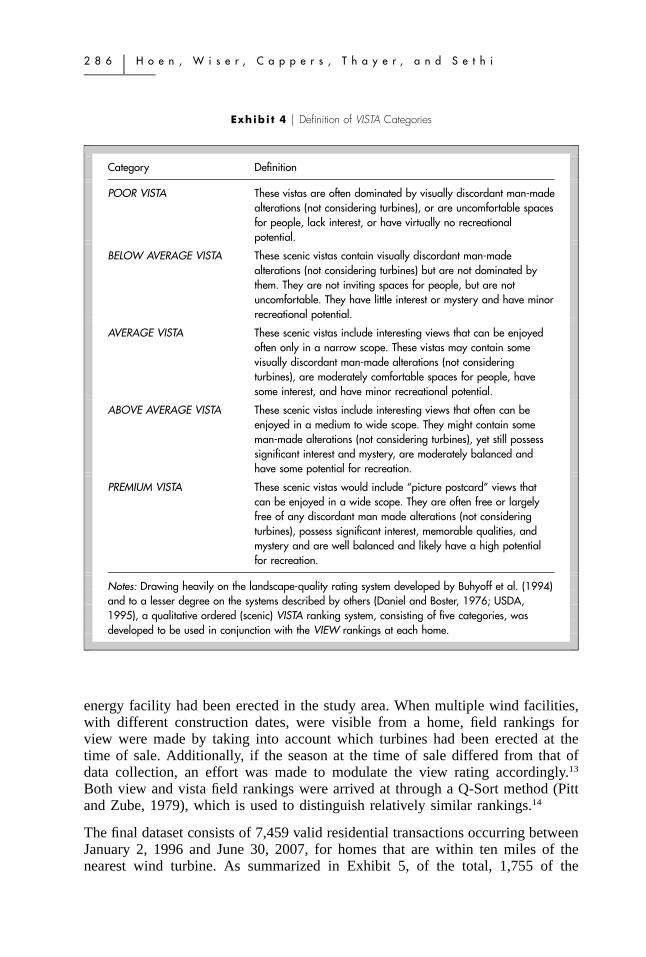
A rating for the quality of the scenic vista (VISTA)10 from each home, absent theexistence of the wind facilities, was also collected in the field. An assessment ofthe quality of the VISTA from each home was required because VIEW and VISTAare expected to be correlated; for example, homes with a PREMIUM VISTA aremore likely to have a wide viewing angle in which wind turbines might also bevisible. Therefore, to accurately measure the impacts of the view of wind turbineson property values a concurrent control for vista (independent of any views ofturbines) was required. Drawing heavily on the landscape-quality rating systemdeveloped by Buhyoff et al. (1994) and to a lesser degree on the systems describedby others (Daniel and Boster, 1976; USDA, 1995), an ordered VISTA rankingsystem consisting of five categories was developed: (1) POOR; (2) BELOWAVERAGE; (3) AVERAGE; (4) ABOVE AVERAGE; and (5) PREMIUM (Exhibit4).11

Field data collection was conducted on a house-by-house basis. Each of the 6,194homes was visited by the same individual to avoid adding bias among fieldrankings. Data collection was conducted in the fall of 2006, and the spring,summer, and fall of 2007 and 2008. Each house was photographed and, whenappropriate, so too were views of turbines and the prominent scenic vista.12 Dataon view were collected only for those homes that sold after at least one wind


Exhibi t 4 � Definition of VISTA Categories

Category Definition

POOR VISTA These vistas are often dominated by visually discordant man-madealterations (not considering turbines), or are uncomfortable spacesfor people, lack interest, or have virtually no recreationalpotential.

BELOW AVERAGE VISTA These scenic vistas contain visually discordant man-madealterations (not considering turbines) but are not dominated bythem. They are not inviting spaces for people, but are notuncomfortable. They have little interest or mystery and have minorrecreational potential.

AVERAGE VISTA These scenic vistas include interesting views that can be enjoyedoften only in a narrow scope. These vistas may contain somevisually discordant man-made alterations (not consideringturbines), are moderately comfortable spaces for people, havesome interest, and have minor recreational potential.

ABOVE AVERAGE VISTA These scenic vistas include interesting views that often can beenjoyed in a medium to wide scope. They might contain someman-made alterations (not considering turbines), yet still possesssignificant interest and mystery, are moderately balanced andhave some potential for recreation.

PREMIUM VISTA These scenic vistas would include ‘‘picture postcard’’ views thatcan be enjoyed in a wide scope. They are often free or largelyfree of any discordant man made alterations (not consideringturbines), possess significant interest, memorable qualities, andmystery and are well balanced and likely have a high potentialfor recreation.

Notes: Drawing heavily on the landscape-quality rating system developed by Buhyoff et al. (1994)and to a lesser degree on the systems described by others (Daniel and Boster, 1976; USDA,1995), a qualitative ordered (scenic) VISTA ranking system, consisting of five categories, wasdeveloped to be used in conjunction with the VIEW rankings at each home.

energy facility had been erected in the study area. When multiple wind facilities,with different construction dates, were visible from a home, field rankings forview were made by taking into account which turbines had been erected at thetime of sale. Additionally, if the season at the time of sale differed from that ofdata collection, an effort was made to modulate the view rating accordingly.13

Both view and vista field rankings were arrived at through a Q-Sort method (Pittand Zube, 1979), which is used to distinguish relatively similar rankings.14

The final dataset consists of 7,459 valid residential transactions occurring betweenJanuary 2, 1996 and June 30, 2007, for homes that are within ten miles of thenearest wind turbine. As summarized in Exhibit 5, of the total, 1,755 of the

Wi

nd

En

er

gy

Fa

ci

li

ti

es

&R

es

id

en

ti

al

Pr

op

er

ti

es

�2

87

JR

ER

�V

ol

.3

3�

No

.3

–2

01

1

Exhibi t 5 � Summary of Transactions across Study Areas and Development Periods

PreAnnouncement

PostAnnouncementPre Construction

1st Year AfterConstruction

2nd Year AfterConstruction

2� Years AfterConstruction Total

Benton/Walla Walla, WA &Umatilla, OR (WAOR)

226 45 76 59 384 790

Howard, TX (TXHC) 169 71 113 131 827 1,311

Custer, OK (OKCC) 484 153 193 187 96 1,113

Buena Vista, IA (IABV) 152 65 80 70 455 822

Lee, IL (ILLC) 115 84 62 71 80 412

Kewaunee/Door, WI (WIKCDC) 44 41 68 62 595 810

Somerset, PA (PASC) 175 28 46 60 185 494

Wayne, PA (PAWC) 223 106 64 71 87 551

Madison/Oneida, NY (MYMCOC) 108 9 48 30 268 463

Madison, NY (NYMC) 59 165 74 70 325 693

TOTAL 1,755 767 824 811 3,302 7,459

Notes: The final dataset consists of 7,459 valid residential transactions occurring between January 2, 1996 and June 30, 2007, for homes that are within 10miles of the nearest wind turbine. Transactions spanned the period prior to the announcement of the decision to build the wind facility to well after thefacility’s construction and are spread across all ten study areas.


transactions occurred prior to wind facility announcement, 764 occurred afterannouncement but before construction, and 4,937 occurred after facilityconstruction. The transactions are arrayed across time and the ten wind facilitystudy areas. A basic summary of the resulting dataset, including the manyindependent variables used in the hedonic models, is contained in Exhibit 6:summary information for the full dataset, as well as the post-construction (homesthat sold after wind facility construction began) subset of the dataset is provided.15

As indicated in Exhibit 6, the mean nominal residential transaction price in thefull sample is $102,968, or $79,114 in 1996 dollars. The average (mean) housein the sample was 46 years old, situated on 1.13 acres, with 1,620 square feet offinished living area above ground, 1.74 bathrooms, and a slightly better thanaverage condition. Of the 4,937 transactions in the sample that occurred after windfacility construction, 730 transactions involved homes that sold with a view of theturbines, with 169 of those transactions involving homes that had a view rankinghigher than MINOR (e.g., MODERATE, SUBSTANTIAL, OR EXTREME). Inaddition, 125 transactions involved homes that sold after construction and that arelocated within a mile of the nearest turbine, with an additional 20 transactionsinvolving homes located within a mile that sold after the facility was announcedbut before construction commenced.

� M o d e l E s t i m a t i o n

A series of hedonic models was estimated to assess whether residential sales priceswere affected by views of and proximity to wind energy facilities in a statisticallymeasurable way. In so doing, the presence of the three potential property valuestigmas associated with wind energy facilities was simultaneously tested for: area,scenic vista, and nuisance. All of the estimated models have four sets ofparameters. One of these sets is associated with the variables of interest(DISTANCE and VIEW), which test for the presence of the three stigmas asdiscussed later, while the other three sets are associated with controls that includehome and site characteristics, study area fixed effects, and spatial adjustments.16

The models differ in their specification and testing of the variables of interest, butuse the same three sets of controls.

The first of these sets of control variables account for home and site-specificcharacteristics such as age of the home (linear and squared), square feet, acres,number of bathrooms and fireplaces, the condition of the home,17 the quality ofthe scenic vista from the home, the presence of central air-conditioning, a stoneexterior, and/or a finished basement, and whether the home is located in a cul-de-sac and/or on a waterfront (Exhibit 6). In the case of the condition (of thehome) and scenic vista variables, the reference cases are average condition andaverage scenic vista, respectively.

The second set, the study area fixed effects variables, include dummy variablesthat control for aggregated study area influences. The estimated coefficients for

Wi

nd

En

er

gy

Fa

ci

li

ti

es

&R

es

id

en

ti

al

Pr

op

er

ti

es

�2

89

JR

ER

�V

ol

.3

3�

No

.3

–2

01

1

Exhibi t 6 � Summary Statistics

Variable Description

All Sales

Mean Std. Dev.

Post-Construction Sales

Mean Std. Dev.

SalePrice Unadjusted sale price of the home (in U.S. dollars). 102,968 64,293 110,166 69,422

SalePrice96 Sale price of the home in 1996 U.S. dollars. 79,114 47,257 80,156 48,906

LN SalePrice96 Natural log of sale price of the home in 1996 U.S. dollars. 11.117 0.58 11.12 0.60

AgeatSale Age of the home at the time of sale. 46 37 47 36

AgeatSale Sqrd Age of the home at the time of sale squared. 3,491 5,410 3,506 5,412

Sqft 1000 Number of finished square feet of above grade (in 1000s). 1.623 0.59 1.628 0.589

Acres Number of acres sold with the residence. 1.128 2.42 1.10 2.40

Baths Number of bathrooms (full bath � 1, half bath � 0.5). 1.738 0.69 1.75 0.70

ExtWalls Stone Home has exterior walls of stone, brick or stucco (Yes � 1,No � 0).

0.307 0.301

CentralAC Home has a central AC unit (Yes � 1, No � 0). 0.507 0.522

Fireplace Number of fireplace openings. 0.390 0.55 0.40 0.55

Cul De SacHome is situated on a cul-de-sac (Yes � 1, No � 0). 0.133 0.136

FinBsmt Finished basement square feet � 50% first floor square feet(Yes � 1, No � 0).

0.197 0.201

Water Front Home shares property line with body of water or river(Yes � 1, No � 0).

0.014 0.018

Cnd Low Condition of the home is Poor (Yes � 1, No � 0). 0.014 0.014

Cnd BAvg Condition of the home is Below Average (Yes � 1, No � 0). 0.070 0.073

Cnd Avg Condition of the home is Average (Yes � 1, No � 0). 0.584 0.552

29

0�

Ho

en

,W

is

er

,C

ap

pe

rs

,T

ha

ye

r,

an

dS

et

hi

Exhibi t 6 � (continued)

Summary Statistics


All Sales

Mean Std. Dev.


Mean Std. Dev.

Cnd AAvg Condition of the home is Above Average (Yes � 1, No � 0.) 0.274 0.293

Cnd High Condition of the home is High (Yes � 1, No � 0). 0.059 0.068

Vista Poor Scenic Vista from the home is Poor (Yes � 1, No � 0). 0.063 0.063

Vista BAvg Scenic Vista from the home is Below Average (Yes � 1,No � 0).

0.577 0.579

Vista Avg Scenic Vista from the home is Average (Yes � 1, No � 0). 0.256 0.253

Vista AAvg Scenic Vista from the home is Above Average (Yes � 1,No � 0).

0.088 0.091

Vista Prem Scenic Vista from the home is Premium (Yes � 1, No � 0). 0.016 0.015

SaleYear Year the home was sold. 2002 2.9 2004 2.3

View None Home sold post-construction with no view of turbines (Yes � 1,No � 0).

0.564 0.852

View Minor Home sold post-construction with Minor View (Yes � 1,No � 0).

0.075 0.114

View Mod Home sold post-construction with Moderate View (Yes � 1,No � 0).

0.014 0.021

View Sub Home sold post-construction with Substantial View (Yes � 1,No � 0).

0.005 0.007

View Extrm Home sold post-construction with Extreme View (Yes � 1,No � 0).

0.004 0.006

Wi

nd

En

er

gy

Fa

ci

li

ti

es

&R

es

id

en

ti

al

Pr

op

er

ti

es

�2

91

JR

ER

�V

ol

.3

3�

No

.3

–2

01

1


Summary Statistics


All Sales

Mean Std. Dev.


Mean Std. Dev.

DISTANCE a Distance to nearest turbine for post-announcement homes,otherwise 0.

2.53 2.59 3.57 1.68

Mile Less 0.57 a Home sold post-announcement and was located within 0.57miles (3000 feet) from nearest turbine (Yes � 1, No � 0).

0.011 0.014

Mile 0.57to1a Home sold post-announcement and was located between 0.57miles (3000 feet) and 1 mile from nearest turbine (Yes � 1,No � 0).

0.009 0.012

Mile 1to3 a Home sold post-announcement and was located between 1and 3 miles from nearest turbine (Yes � 1, No � 0).

0.316 0.409

Mile 3to5 a Home sold post-announcement and was located between 3and 5 miles from nearest turbine (Yes � 1, No � 0).

0.295 0.390

Mile Gtr5 a Home sold post-announcement and was located at least 5miles from nearest turbine (Yes � 1, No � 0).

0.134 0.176

Notes: The mean residential transaction price in the full sample is $102,968 (nominal) and $79,114 ($1996), which represents a house over 46 years old,situated on 1.13 acres, with 1,620 square feet of finished living area above ground, 1.74 bathrooms, and a slightly better than average condition.a ‘‘All Sales’’ mean and standard deviation DISTANCE and DISTANCE fixed effects variables (e.g., Mile 1to3) include transactions that occurred after facility‘‘announcement’’ and before ‘‘construction’’ as well as those that occurred post-construction.


this group of variables capture the combined effects of school districts, tax rates,crime, and other location influences across a study area. Although this approachgreatly simplifies the estimation of the model, interpreting the coefficients can bedifficult because of the myriad influences captured by these study area fixed effectsvariables. The reference category is the Washington/Oregon (WAOR) study area.Because there is no intent to focus on the coefficients of the study area fixed effectvariables, the reference case is arbitrary; further, the results for the other variablesin the model are completely independent of this choice. Although models usingstudy area fixed effects are presented here, the hedonic results are robust to thealternative of including school district and census tract variables in addition to thestudy area fixed effects variables, as is discussed below in the robustness testssection.

The third set controls for spatial dependence. Since the sales price of a home isoften influenced by the sales prices of homes in the same neighborhood, ignoringthe underlying spatial dependence in the data could bias the OLS estimates (Espey,Fakhruddin, Gering, and Lin (2007). Spatial dependence among the prices ofhomes can take two forms: spatial autocorrelation and spatial heterogeneity. Theformer captures the direct effect of neighboring properties on the value of a givenproperty, whereas the latter accounts for the correlation among unobservablefactors that affect property values in a given neighborhood. The inclusion of studyarea fixed effects likely reduces spatial heterogeneity, though further study of thisissue is warranted.18 Spatial autocorrelation, meanwhile, is addressed by includingas a control variable a spatially weighted neighbor’s sales price (N) for eachtransaction, which was calculated using the estimated (i.e., predicted) sales pricesof the five nearest neighbors within the six preceding months. The predicted salesprice is used to offset any potential endogeneity associated with the neighbor’sprice variable. The two-stage estimation process is similar to that proposed inKelejian and Prucha (1998). The definition of ‘‘nearest neighbors’’ was chosen tomimic the selection process of a set of comparables by appraisers and/or realtors.19

M o d e l 1

As noted earlier, the dataset consists of 7,459 residential transactions, of which2,522 transactions occurred before the wind facility was constructed. The analysisbegins with the simplest of the hedonic models in which only the 4,937 post-construction transactions are used. As is common in the literature (Malpezzi, 2002;Simons and Saginor, 2006; Sirmans, Macdonald, and Macpherson, 2006), a semi-log functional form is used where the dependent variable, the (natural log of )sales price (P), is measured in market-specific inflation-adjusted (1996) dollars.

The literature on environmental disamenities often uses a continuous variable forthe distance from the home to the disamenity (e.g., Sims, Dent, and Oskrochi,2008). A number of different functional forms can be used for a continuousdistance variable, including linear, inverse, cubic, quadratic, logarithmic, andspline. Of the forms that were considered, the linear spline seemed most


J R E R � V o l . 3 3 � N o . 3 – 2 0 1 1

appropriate for this purpose. Spline functions are used when it is assumed that amarginal change in sale price per unit of distance is not constant across alldistances from a disamenity and that those effects should be estimated separately.This form dovetails well with area and nuisance stigma definitions, wherein aneffect based on distance can be estimated across the entire sample of homes (areastigma) and separately for those homes inside of one mile (nuisance stigma).20

Therefore, the following model is estimated:

ln(P) � � � � N � � S � � X � � VIEW� � �0 1 2 3 4s k v

� � DISTANCE � � ((DISTANCE � 1) � LT1MILE) � �,5 6

(1)

where N is the spatially weighted neighbors’ predicted sales price, S is the vectorof s study area fixed effects variables (e.g., TXHC, OKCC), X is a vector of khome and site characteristics, (e.g., acres, square feet), VIEW is a vector of vcategorical turbine view variables (e.g., MINOR, MODERATE), DISTANCE is themeasurement (in miles) from the home to the nearest turbine at the time of sale,and LT1MILE equals 1 when the distance is less than one mile, and 0 otherwise,�0 is the constant or intercept across the full sample, �1 is a parameter estimatefor the spatially weighted neighbor’s predicted sales price, �2 is a vector of sparameter estimates for the study area fixed effects as compared to homes sold inthe Washington/Oregon (WAOR) study area, �3 is a vector of k parameterestimates for the home and site characteristics, �4 is a vector of v parameterestimates for the VIEW variables as compared to homes sold with no view of theturbines, �5 is a parameter estimate for the effect distance has on sale price acrossall homes, �6 is a parameter estimate for the additive effect distance has on saleprice for those homes inside of one mile, and � is a random disturbance term.Also note that both VIEW and DISTANCE appear in the model together becausea home’s value may be affected in part by the magnitude of the view of the windturbines, and, in part by the distance from the home to those turbines; validationof this assumption is discussed later when summarizing various robustness teststhat were performed.

In this model, and all subsequent models, scenic vista stigma is tested for via thecoefficients of the view variable, which are expected to be negative, significant,and monotonically decreasing from EXTREME to MINOR. The effect of areastigma is expected to be captured through the variable DISTANCE and the effectof nuisance stigma through the variable (DISTANCE � 1)*LT1MILE as it hasbeen in the previous literature (e.g., Thayer, Albers, and Rahmatian (1992). Ifthese latter two stigmas exist, the coefficients of these variables are expected tobe positive and significant, indicating an increase in selling prices for each milethe homes are further from the wind turbines.21


M o d e l 2

Though the continuous form of DISTANCE, as used in Model 1, is consistent withthe previous literature, it imposes a rigid structure on the dataset that may lead tospecification errors. Model 2 relaxes this rigidity by measuring distance incategorical form. In this model, the reference category for distance is the set oftransactions for homes that are situated outside of five miles from the nearest windturbine. This reference category was because these homes are least likely to beaffected by the presence of the wind facilities.22 Other than this change, the datasetused for the estimation, the list of controls, and the specification of the viewvariable remain unchanged relative to Model 1. Therefore, the following model isestimated:

ln(P) � � � � N � � S � � X� �0 1 2 3s k

� � VIEW � � DISTANCE � �, (2)� �4 5v d

where DISTANCE is a vector of d categorical distance to turbine variables (e.g.,less than 3,000 feet, between 3,000 feet and one mile), the reference categorybeing homes situated outside of five miles. All other variables are as described inModel 1.

Since the view variable is unchanged, it is expected to capture the effect of scenicvista stigma in a manner identical to Model 1. It is assumed that nuisance effectsare largely concentrated within one mile of the nearest wind turbine, while areaeffects may occur to a varying degree all homes within a five-mile radius of thewind facility. Therefore, property value effects as identified by the coefficients ofthe distance variables inside of one mile (e.g., inside 0.57 mile, and between 0.57mile and 1 mile) can be interpreted as a combination of area and nuisance stigmas,while the coefficients of variables outside of one mile can be interpreted as onlyreflecting area sigma effects. All coefficients are expected to be negative andmonotonically decreasing as the distance band increases.

M o d e l 3

Though Model 2 relaxes some of the structural rigidity of Model 1, it implicitlyassumes that the area stigma effects die out completely after a distance of fivemiles from a wind facility. The validity of this assumption can be tested bycomparing the prices of homes sold before the construction of the wind facilityto those sold after. Further, by using only the post-construction data, both Models1 and 2 ignore the possible anticipated effect of wind facility construction by notusing data from the post-announcement pre-construction period. Previous research


J R E R � V o l . 3 3 � N o . 3 – 2 0 1 1

suggests that property value effects might be very strong during this period, duringwhich an assessment of actual impacts is not possible and buyers and sellers maytake a risk-adverse and conservative stance (Wolsink, 1989). Model 3 addressesboth of these issues by using the entire dataset (7,459 transactions), includinghomes that sold well before the facility was announced, through the period afterannouncement yet prior to construction, and continuing to well after construction.The following specification is used:

ln(P) � � � � N � � S � � X� �0 1 2 3s k

� � VIEW � POSTCON� 4v

� � DISTANCE � POSTANC � �, (3)� 5d

where POSTCON is one if the sale occurred after the wind facility was constructed(zero otherwise), POSTANC is one if the sale occurred after the wind facility wasannounced (zero otherwise), and all other variables are as defined in equation (2).In this model, all pre-construction sales serve as the reference category for view,and all pre-announcement sales serve as the reference category for distance. Thismodel, therefore, also serves as a robustness check on the reference categoriesused in Models 2 and 3: by comparing the coefficients for the DISTANCE andVIEW variables from all three models, a comparison can be made between thereference categories and therefore their appropriateness for use.

In this model, the scenic vista stigma is expected to be captured via the variableVIEW*POSTCON, and the area and nuisance stigmas through the interactionvariable DISTANCE*POSTANC. The coefficients of the VIEW and DISTANCEvariables, as with previous models, are expected to be negative and monotonicallyordered.

M o d e l 4

Model 3 allows all post-announcement sales to be potentially impacted by areaand nuisance stigma, and therefore might be considered an improvement overModel 2, but it makes the assumption that the marginal effect of distance isconstant across all time periods. As discussed previously, however, there is someevidence that property value impacts may be particularly strong after theannouncement of a disamenity, but then may fade with time as the communityadjusts to the presence of that disamenity (e.g., Wolsink, 1989). Model 4 allowsfor an investigation of how different periods of the wind power developmentprocess affect estimates for the impact of distance on sales prices. The followingspecification is used:


ln(P) � � � � N � � S � � X� �0 1 2 3s k

� � VIEW � POSTCON� 4v

� � (DISTANCE � PERIOD) � �, (4)� 5y

where PERIOD is a vector of development periods. The PERIOD variable containssix categories: (1) more than two years before announcement; (2) less than twoyears before announcement; (3) after announcement but before construction; (4)less than two years after construction; (5) between two and four years afterconstruction; and (6) more than four years after construction. Further, in contrastto Models 2 and 3, Model 4 collapses the two distance categories inside of onemile into a single ‘‘less than one mile’’ group to ensure that reasonably largenumbers of transactions (e.g., ��30) were used to estimate effects in eachperiod.23 Therefore, in this model, the DISTANCE variable contains four differentlevels: (1) less than one mile; (2) between one and three miles; (3) between threeand five miles; and (4) outside of five miles. Consequently, the DISTANCE �PERIOD interaction created 24 distinct variables.

This model’s reference case consists of transactions that occurred more than twoyears before the facility was announced for homes that were situated more thanfive miles from where the turbines were ultimately constructed. It is assumed thatthe value of these homes would not be affected by the future presence of the windfacility. The VIEW parameters, although included in the model, are not interactedwith PERIOD.24

Although the comparisons of these categorical variables between different distanceand period categories might be interesting, it is the comparison of coefficientswithin each period and distance category that is the focus of this model. Suchcomparisons, for example, allow one to compare how the average value of homesinside of one mile that sold two years before announcement compare to theaverage value of homes inside of one mile that sold in later periods.

� R e s u l t s

The range of adjusted R2 values for the four models is between 0.75 and 0.77(Exhibit 7).25 The sign and magnitudes of the site and home control variables areconsistent with a priori expectations, are stable across all four hedonic models,and all are statistically significant at the 1% level (Exhibit 7). These results canbe benchmarked to other research. Specifically, Sirmans, Macpherson, and Zietz(2005) and Sirmans, Mcdonald, and Macpherson (2006) conducted a meta-analysis of 64 hedonic studies carried out in multiple locations in the U.S. duringmultiple time periods, and investigated the coefficients of ten commonly-used

Wi

nd

En

er

gy

Fa

ci

li

ti

es

&R

es

id

en

ti

al

Pr

op

er

ti

es

�2

97

JR

ER

�V

ol

.3

3�

No

.3

–2

01

1

Exhibi t 7 � Model Summary and Control Variable Results

Model 1 Model 2 Model 3 Model 4

Number of Cases 4,937 4,937 7,459 7,459

Number of Predictors 35 37 39 56

F-Statistic 468 443 580 404

Adj. R2 0.77 0.77 0.75 0.75

Intercept 7.63 (0.18)** 7.62 (0.18)** 9.08 (0.14)** 9.11 (0.14)**

Spatial Control—Post Con 0.29 (0.02)** 0.29 (0.02)**

Spatial Control—All Sales 0.16 (0.01)** 0.16 (0.01)**

AgeatSale �0.0059 (0.00)** �0.0059 (0.00)** �0.007 (0.00)** �0.007 (0.00)**

AgeatSale Sqrd 0.00002 (0.00)** 0.00002 (0.00)** 0.00003 (0.00)** 0.00003 (0.00)**

Sqft 1000 0.28 (0.01)** 0.28 (0.01)** 0.28 (0.01)** 0.28 (0.01)**

Acres 0.02 (0.00)** 0.02 (0.00)** 0.02 (0.00)** 0.02 (0.00)**

Baths 0.09 (0.01)** 0.09 (0.01)** 0.08 (0.01)** 0.08 (0.01)**

ExtWalls Stone 0.21 (0.02)** 0.21 (0.02)** 0.21 (0.01)** 0.21 (0.01)**

CentralAC 0.09 (0.01)** 0.09 (0.01)** 0.12 (0.01)** 0.12 (0.01)**

Fireplace 0.11 (0.01)** 0.11 (0.01)** 0.11 (0.01)** 0.12 (0.01)**

FinBsmt 0.08 (0.02)** 0.08 (0.02)** 0.09 (0.01)** 0.09 (0.01)**

Cul De Sac 0.1 (0.01)** 0.1 (0.01)** 0.09 (0.01)** 0.09 (0.01)**

Water Front 0.34 (0.04)** 0.33 (0.04)** 0.35 (0.03)** 0.35 (0.03)**

Cnd Low �0.44 (0.05)** �0.45 (0.05)** �0.43 (0.04)** �0.43 (0.04)**

Cnd BAvg �0.24 (0.02)** �0.24 (0.02)** �0.21 (0.02)** �0.21 (0.02)**

Cnd Avg Omitted (Omitted) Omitted (Omitted) Omitted (Omitted) Omitted (Omitted)

29

8�

Ho

en

,W

is

er

,C

ap

pe

rs

,T

ha

ye

r,

an

dS

et

hi


Model Summary and Control Variable Results


Cnd AAvg 0.13 (0.01)** 0.14 (0.01)** 0.13 (0.01)** 0.13 (0.01)**

Cnd High 0.23 (0.02)** 0.23 (0.02)** 0.22 (0.02)** 0.22 (0.02)**

Vista Poor �0.21 (0.02)** �0.21 (0.02)** �0.25 (0.02)** �0.25 (0.02)**

Vista BAvg �0.08 (0.01)** �0.08 (0.01)** �0.09 (0.01)** �0.09 (0.01)**

Vista Avg Omitted (Omitted) Omitted (Omitted) Omitted (Omitted) Omitted (Omitted)

Vista AAvg 0.10 (0.02)** 0.10 (0.02)** 0.10 (0.01)** 0.10 (0.01)**

Vista Prem 0.13 (0.04)** 0.13 (0.04)** 0.09 (0.03)** 0.09 (0.03)**

WAOR Omitted (Omitted) Omitted (Omitted) Omitted (Omitted) Omitted (Omitted)

TXHC �0.75 (0.03)** �0.75 (0.03)** �0.82 (0.02)** �0.82 (0.02)**

OKCC �0.44 (0.02)** �0.44 (0.02)** �0.53 (0.02)** �0.52 (0.02)**

IABV �0.24 (0.02)** �0.24 (0.02)** �0.31 (0.02)** �0.3 (0.02)**

ILLC �0.09 (0.03)** �0.09 (0.03)** �0.05 (0.02)* �0.04 (0.02)*

WIKCDC �0.14 (0.02)** �0.14 (0.02)** �0.17 (0.01)** �0.17 (0.02)**

PASC �0.3 (0.03)** �0.31 (0.03)** �0.37 (0.03)** �0.37 (0.03)**

PAWC �0.07 (0.03)** �0.07 (0.03)** �0.15 (0.02)** �0.14 (0.02)**

NYMCOC �0.2 (0.03)** �0.2 (0.03)** �0.25 (0.02)** �0.25 (0.02)**

NYMC �0.14 (0.02)** �0.15 (0.02)** �0.15 (0.02)** �0.15 (0.02)**

Notes: The sign and magnitudes of the home and site, study area, and spatial control variables are consistent with a priori expectations, are stable across allfour hedonic models, and all are statistically significant at the 1% level. Of note are the scenic vista and cul-de-sac coefficients, indicating strong relationshipsbetween visual and proximate characteristics (not considering turbines) and sale prices. Standard errors are in parentheses.*Significant at or above the 5% level.**Significant at or above the 1% level.


J R E R � V o l . 3 3 � N o . 3 – 2 0 1 1

characteristics, seven of which were included in our models. The similaritiesbetween the mean coefficients (i.e., the average across all 64 studies) reported bythese studies and those estimated in the present study are striking. For example,the effect of square feet (in 1000s) on log of sales price was estimated to be 0.28across all four of the hedonic models presented here and Sirmans et al. (2005,2006) provide an estimate of 0.34, while the effect of acres was similarly estimated[0.02 to 0.03, present study and Sirmans et al. (2005, 2006), respectively]. Further,age at the time of sale (�0.006 to �0.009), bathrooms (0.09 to 0.09), central air-conditioning (0.09 to 0.08), and fireplaces (0.11 to 0.09) all similarly compare.As a group, the estimates in the present study differ in all cases by no more thana third of the Sirmans et al. (2005, 2006) mean estimate’s standard deviation.

The coefficients for the spatial control (‘‘Spatial Control – Post Con’’ in Models1 and 2, ‘‘Spatial Control–All Sales’’ in Models 3 and 4) are also significant atthe 1% level, indicating a strong relationship between the predicted value of theneighbors’ selling prices and those of the subject home. In addition, all the studyarea fixed effects coefficients are significant at the 1% level. The omitted studyarea category (WAOR), which had the highest overall median house prices (theWAOR value is $169,177 whereas the remainder of the sample is $120,256), wasspecifically chosen so that all of the study area fixed effects coefficients wouldhave negative signs. As noted earlier, this choice was arbitrary and has no impacton the remainder of the results.

Of particular interest are the coefficient estimates for scenic vista (VISTA). Homeswith a scenic vista rated as poor are found to sell for 21% to 25% less on averagethan homes with an average rating, while homes with a premium vista sell for9% to 13% more than homes with an average rating. In all four of the models,differences between homes with an average scenic vista and homes with otherscenic vistas are significant at the 1% level. Based on these results, it is evidentthat the quality of the scenic vista is capitalized into sales prices, and that thequalitative VISTA variable is able to effectively capture these effects. Tobenchmark these results, they were compared to the few studies that haveinvestigated the contribution of inland scenic vistas to sales prices. Benson,Hansen, and Schwartz (2000) found that a mountain vista increases sales price by8%, while Bourassa, Hoesli, and Sun (2004) found that wide inland vistas increasesales price by 7.6%. These both compare favorably to the results for above averageand premium rated vista estimates presented in Exhibit 7.

S c e n i c V i s t a S t i g m a

Scenic vista stigma is defined as a concern that a home may be devalued becauseof the view of a wind energy facility, and the potential impact of that view on anotherwise scenic vista. This concern is premised on the notion that home valuesare, in part, derived from the quality of what can be viewed from the property.

As mentioned earlier, the results from all four models demonstrate persuasivelythat the quality of the scenic vista (the VISTA variable) does impact sales prices.


Along the same lines, homes in the sample with water frontage or situated on acul-de-sac sell for 33% to 35% more and 9% to 10% more, on average,respectively, than those homes that lack these characteristics, differences that aresignificant at or above the 1% level. Taken together, these results demonstrate thathome buyers and sellers consistently take into account what can be seen from thehome when sales prices are established, and that the models presented in thispaper are able to clearly identify those impacts when they exist.26

Despite this finding, the models are unable to identify any evidence of a scenicvista stigma associated with the wind facilities in the sample (Exhibit 8).Specifically, the 25 homes with extreme views in the sample, where the home siteis ‘‘unmistakably dominated by the [visual] presence of the turbines,’’ are notfound to have statistically different selling prices than either those that sold in thesame period but which did not have a view (Models 1 and 2) or that sold priorto the wind facility’s construction (Models 3 and 4). The same finding holds forthe 106 and 561 homes that were rated as having either moderate or minor viewsof the wind turbines, respectively.

A r e a S t i g m a

Area stigma is defined as a concern that the general area surrounding a windenergy facility will appear more developed, which may adversely affect homevalues in the local community regardless of whether any individual home has aview of the wind turbines. Though these impacts might be expected to beespecially severe at close range to the turbines, the impacts could conceivablyextend for a number of miles around a wind facility. Modern wind turbines arevisible from well outside of five miles in many cases, so if an area stigma exists,it is possible that all of the homes in the study areas inside of five miles couldbe affected. We focus on transactions of homes located outside of one mile todistinguish this generalized area stigma effect from nuisance effects.

The presence of area stigmas was tested in each of the four models (Exhibit 8).Model 1 uses a continuous linear distance function and finds a relatively small(0.004) and non-significant (p-value � 0.25) relationship between distance (inmiles) from the nearest turbine and the value of residential properties for the 4,937transactions occurring after construction commenced. Similarly, Model 2 finds nostatistical difference between the sales prices of homes located more than fivemiles from the turbines and those located in any nearer distance band. Likewise,in Model 3, the coefficients of DISTANCE for homes that sold outside of one mileafter an announcement are essentially no different to those that sold prior to anannouncement, with coefficients ranging between 0.00 and 0.01, none of whichare statistically significant. Further, homes that sold after facility construction butthat had no view of the turbine are found to appreciate in value, after adjustingfor inflation, when compared to homes that sold before wind facility construction(0.02, p-value � 0.06); any area stigma effect that impacts the general areasurrounding wind facilities should be reflected as a negative coefficient for this

Wi

nd

En

er

gy

Fa

ci

li

ti

es

&R

es

id

en

ti

al

Pr

op

er

ti

es

�3

01

JR

ER

�V

ol

.3

3�

No

.3

–2

01

1

Exhibi t 8 � Results for Variable of Interest


No View Omitted (Omitted) Omitted (Omitted) 0.02 (0.01) Omitted (Omitted)

Minor View �0.01 (0.01) �0.01 (0.01) 0.00 (0.02) �0.02 (0.01)

Moderate View 0.01 (0.03) 0.02 (0.03) 0.03 (0.03) 0.00 (0.03)

Substantial View �0.01 (0.07) �0.01 (0.07) 0.03 (0.07) 0.01 (0.07)

Extreme View 0.04 (0.1) 0.02 (0.09) 0.06 (0.08) 0.04 (0.07)

Pre-Construction Sales Omitted (Omitted)

Inside 3000 Feet �0.05 (0.06) �0.06 (0.05)

Between 3000 Feet and 1 Mile �0.05 (0.05) �0.08 (0.05)

Between 1 and 3 Miles 0.00 (0.02) 0.00 (0.01)

Between 3 and 5 Miles 0.02 (0.01) 0.01 (0.01)

Outside 5 Miles Omitted (Omitted) 0.00 (0.02)

Pre-Announcement Sales Omitted (Omitted)

DISTANCE 0.004 (0.00)

DISTANCE*LT1MILE 0.086 (0.11)Inside 1 Mile Gtr2Yr PreAnc �0.13 (0.06)*

Lt2Yr PreAnc �0.10 (0.05)PostAnc PreCon �0.14 (0.06)*Lt2Yr PostCon �0.09 (0.07)Btw2 4Yr PostCon �0.01 (0.06)Gtr4Yr PostCon �0.07 (0.08)

30

2�

Ho

en

,W

is

er

,C

ap

pe

rs

,T

ha

ye

r,

an

dS

et

hi


Results for Variable of Interest


Between 1–3 Miles Gtr2Yr PreAnc �0.13 (0.06)*Lt2Yr PreAnc 0.00 (0.03)PostAnc PreCon �0.02 (0.03)Lt2Yr PostCon 0.00 (0.03)Btw2 4Yr PostCon 0.01 (0.03)Gtr4Yr PostCon 0.00 (0.03)

Between 3–5 Miles Gtr2Yr PreAnc 0.00 (0.04)Lt2Yr PreAnc 0.00 (0.03)PostAnc PreCon 0.00 (0.03)Lt2Yr PostCon 0.02 (0.03)Btw2 4Yr PostCon 0.01 (0.03)Gtr4Yr PostCon 0.01 (0.03)

Outside 5 Miles Gtr2Yr PreAnc Omitted (Omitted)Lt2Yr PreAnc �0.03 (0.04)PostAnc PreCon �0.03 (0.03)Lt2Yr PostCon �0.03 (0.03)Btw2 4Yr PostCon 0.03 (0.03)Gtr4Yr PostCon 0.01 (0.03)

Notes: Across four different hedonic models, the results are consistent: neither the view of the wind facilities nor the distance of the home to those facilities isfound to have a statistically significant effect on home sales prices. These results are strengthened in light of the statistically significant relationships found fornon-turbine related visual and proximate characteristics. Standard errors are in parentheses.*Significant at or above the 5% level.**Significant at or above the 1% level.


J R E R � V o l . 3 3 � N o . 3 – 2 0 1 1

parameter. It should also be noted that the stability of the distance coefficientsacross Models 2 and 3, where different reference cases are used, reinforces boththe stability of the models and the appropriateness of the reference case selection.

Perhaps a more direct test of area stigma comes from Model 4. In this model,homes in all distance bands outside of one mile and that sold after wind facilityannouncement are found to sell, on average, for prices that are not statisticallydifferent from sales that occurred more than two years prior to a wind facilityannouncement.

To summarize, there is little evidence of the existence of an area stigma amongthe homes in this sample. On average, homes in these study areas are notdemonstrably and measurably stigmatized by the arrival of a wind facility basedon area stigma, regardless of when they sold in the wind power developmentprocess and regardless of whether those homes are located one mile or five milesaway from the nearest wind facility.

N u i s a n c e S t i g m a

Nuisance stigma is defined as any adverse impacts, such as sound and shadowflicker, which might uniquely affect residents of homes in close proximity to windturbines, thereby leading to a potential reduction of home sales prices.

The results of Model 1 (Exhibit 8), where a continuous linear function is estimatedfor only those homes within one mile, imply a 4.1% reduction in the values ofhomes located one half mile away from the wind facility, and a 6.4% reductionfor those within one quarter of a mile, though these results are not statisticallysignificant.27 Similarly, Model 2 finds that those homes within 3,000 feet and thosebetween 3,000 feet and one mile of the nearest wind turbine sold for roughly 5%less than similar homes located more than five miles away that sold in the samepost-construction period. Again, these differences are not statistically significant(p-values � 0.40 and 0.30, respectively). In Model 3, when all transactionsoccurring after wind facility announcement are assumed to potentially beimpacted, and a comparison is made to the average of all transactions occurringpre-announcement, the adverse impacts are estimated to be �6% (p-value � 0.23)and �8% (p-value � 0.08), respectively.

Though none of these results are statistically significant, they are possiblyconsistent with the presence of a nuisance stigma. Model 4, however, providesthe clearest picture of these findings, and demonstrates that these effects are notlikely to have been caused by the presence of the wind facilities. As is illustratedin Exhibit 9, homes that sold prior to a wind facility announcement, but situatedwithin one mile of the eventual location of the turbines, sold, on average, forbetween 10% and 13% less than homes that sold in the same time period butlocated more than five miles away. Therefore, the homes nearest the wind facility’seventual location were depressed in value, in comparison to homes further away,prior to the announcement of the facility. Moreover, comparing the sales prices


Exhibi t 9 � Results from Model 4

-25%

-20%

-15%

-10%

-5%

0%

5%

10%

15%

20%

25%

More Than2 YearsBefore

Announcement

Less Than2 YearsBefore

Announcement

AfterAnnouncement

BeforeConstruction

Less Than2 Years

AfterConstruction

Between2 and 4 Years

AfterConstruction

More Than4 Years

AfterConstruction

Ave

rage

Per

cent

age

Diff

eren

ces

The reference category consists of transactions of homes situated more than five miles from where the nearestturbine would eventually be located and that occurred more than two years before announcement of the facility

Price Changes Over TimeAverage percentage difference in sales prices as compared to reference category

Less Than 1 Mile Between 1 and 3 Miles

Between 3 and 5 Miles Outside 5 Miles

Reference CategoryOutside of 5 MilesMore Than 2 Years

Before Announcement

POST CONSTRUCTIONPRE ANNOUNCEMENT

Homes that sold prior to wind facility announcement, but situated within one mile of the eventual location of theturbines, sold, on average, for between 10% and 13% less than homes that sold in the same time period butlocated more than five miles away. Therefore, the homes nearest the wind facility’s eventual location were de-pressed in value prior to the announcement of the facility in comparison to homes further away.

of the homes located within a mile of the turbines between those that transactedmore than two years prior to the facilities’ announcement and those that sold inlater periods (e.g., after announcement or after construction), as is shown inExhibit 10, differences were statistically indistinguishable from pre-announcementlevels. In other words, relative prices did not fall after the announcement andeventual construction of the wind facility for this sample of homes.

The weak (i.e., not statistically significant) evidence of a nuisance stigma foundin Models 1–3 appear to be a reflection of depressed home prices that precededthe construction of the relevant wind facilities, rather than a reaction to theturbines. If construction of the wind facilities was downwardly influencing thesales prices of these homes, as might be deduced from Models 1, 2, or 3 alone,a diminution in the inflation-adjusted price would be seen as compared to pre-announcement levels in Model 4. Instead, an increase (albeit not-statisticallysignificant) is observed. As such, no persuasive evidence of a nuisance stigma isapparent in this sample.

Wi

nd

En

er

gy

Fa

ci

li

ti

es

&R

es

id

en

ti

al

Pr

op

er

ti

es

�3

05

JR

ER

�V

ol

.3

3�

No

.3

–2

01

1

Exhibi t 10 � Results from Equality Test of Model 4 Coefficients

�2 YearsBeforeAnnouncement

�2 YearsBeforeAnnouncement

AfterAnnouncementBeforeConstruction

�2 YearsAfterConstruction

2–4 YearsAfterConstruction

�4 YearsAfterConstruction

Less Than 1 Mile Reference 0.03 (0.45) �0.01 (�0.13) 0.04 (0.56) 0.12 (1.74) 0.06 (0.88)

Between 1 and 3 Miles Reference 0.04 (1.92) 0.02 (0.86) 0.05 (2.47)* 0.05 (2.27)* 0.04 (1.82)

Between 3 and 5 Miles Reference 0.01 (0.37) 0.01 (0.34) 0.02 (0.77) 0.02 (0.78) 0.02 (0.79)

Outside of 5 Milesa Reference �0.04 (�0.86) �0.03 (�0.91) �0.03 (�0.77) 0.03 (0.81) 0.01 (0.36)

Notes: A comparison of the sales prices for the homes located within a mile of the turbines which transacted more than two years prior to the facilities’announcement and those that sold in later periods (e.g., after announcement or after construction) produced differences that were statisticallyindistinguishable from pre-announcement levels. In other words, relative prices did not fall after the announcement and eventual construction of the windfacility for this sample of homes. Numbers in parentheses are t -statistics. Numbers represent the differences between coefficients in the target temporalcategory and those in the reference temporal category (more than two years before announcement) for the same distance band.*Significant at or above the 5% level.**Significant at or above the 1% level.a For homes outside of five miles, the coefficient differences are equal to the coefficients in Model 4, and therefore the t -values were produced via the OLS.


� R o b u s t n e s s Te s t s

The results reported in Exhibits 8–10 suggest that wind facilities in this sampledo not demonstrably cause scenic vista, area, or nuisance stigmas. Because thisresult is somewhat counter-intuitive and possibly controversial, several alternativemodel specifications to the four presented earlier were estimated to determinewhether or not the results were robust. These alternative specifications included:(1) interacting the study area fixed effects variables with the home and sitecharacteristics to mimic the estimation of separate regressions for each study area;(2) replacing the study area fixed effects variables with alternative locationmeasures [specifically, census tract and school district delineations, the importanceof which is discussed in Seo and Simons (2009)]; (3) including additional micro-spatial variables in the models (specifically, distance to nearest highway ramp andproximity to a major road); (4) omitting either VIEW or DISTANCE from themodel to explore potential collinearity between these variables; (5) removing thevariable for the spatially weighted sales price of the five nearest neighbors (SpatialControl – Post Con); (6) including five outlier and influential observations thathad previously been removed from the dataset (as discussed in Hoen et al., 2009);(7) including a quantitative measurement of view (pct vis) constructed from thetotal number of turbines visible and the distance of the home to the nearest windturbine28 rather than using the qualitative view categories; and (8) adding fixedeffects variables for the year in which the home sold.

Key results for these robustness checks are presented in Exhibit 11. In the interestof brevity, only Model 2 is used with these alternative specifications, and only theestimated coefficients on two view categories (SUBSTANTIAL and EXTREME)and two distance categories (within 3,000 feet and 3,000 feet to one mile) arereported (although all were investigated). The re-estimated models, unlessotherwise noted, include all of the same control variables and variables of interestas Model 2 specified above.

Exhibit 11 reveals that the estimated coefficients for the robustness models aresimilar in magnitude to the baseline Model 2 estimates (presented at the top ofExhibit 11 for comparison purposes) and none are statistically different from zero(this also holds for the other variables that are not presented). The results aretherefore robust to pooling the data across study areas; alternative locationmeasures; the inclusion/exclusion of additional micro-spatial, neighbor’s price,and/or year fixed effects variables; the omission of either set of variables ofinterest (DISTANCE or VIEW); the inclusion of previously omitted outliers andinfluential observations; and an alternative, quantitative measure of the VIEWvariable. In addition, although not shown here, the results of Model 1 are robustto various distance functions, and the full set of results are consistent with repeatsales and sales volume models [all of which are presented in Hoen et al. (2009),along with several other robustness tests not otherwise mentioned here].

Wi

nd

En

er

gy

Fa

ci

li

ti

es

&R

es

id

en

ti

al

Pr

op

er

ti

es

�3

07

JR

ER

�V

ol

.3

3�

No

.3

–2

01

1

Exhibi t 11 � Robustness Test Results

Substantial View Extreme ViewInside 3,000Feet

Between3,000 Feetand 1 Mile pct vis

Model 2 �0.01 (0.07) 0.02 (0.09) �0.05 (0.06) �0.05 (0.05)

Robustness Models

Interactions Between Study Area andHome and Site Characteristics Included

0.002 (0.07) 0.01 (0.09) �0.05 (0.06) �0.06 (0.05)

Census Tract and School DistrictDelineations Included

0.03 (0.06) 0.03 (0.08) �0.07 (0.06) �0.02 (0.05)

Micro Spatial Effects—Ramp Distanceand Major Roads Included

0.02 (0.06) 0.02 (0.08) �0.02 (0.06) 0.03 (0.05)

Spatial Control (Nearest Neighbor)Omitted

�0.03 (0.07) �0.006 (0.09) �0.07 (0.06) �0.06 (0.05)

View Variables Omitted �0.04 (0.04) �0.06 (0.05)

Distance Variables Omitted �0.04 (0.06) �0.03 (0.06)

Five Outlier and Influencer Cases Included �0.03 (0.06) 0.02 (0.09) �0.02 (0.06) �0.05 (0.05)

Percent Visible (Quantitative ViewVariable) Tested

�0.09 (0.06) �0.06 (0.04) 0.43 (0.23)

Year Dummies Included �0.01 (0.07) 0.02 (0.09) �0.05 (0.06) �0.05 (0.05)

Notes: The results are consistent across a variety of model and sample specifications. The estimated coefficients for the robustness models are similar inmagnitude to the baseline Model 2 estimates (presented at the top of this table for comparison purposes) and none are statistically different from zero (thisalso holds for the other variables that are not presented in this table). Standard errors are in parentheses.*Significant at or above the 5% level.**Significant at or above the 1% level.


� C o n c l u s i o n

This paper has investigated the potential impacts of wind energy facilities on thesales prices of residential properties that are in proximity to and/or that have aview of those wind facilities. In so doing, three different potential impacts of windfacilities on property values have been identified and analyzed: scenic vista stigma,area stigma, and nuisance stigma. The results are based on the most comprehensivedata on and analysis of the subject to date. Across various model specificationsand after a number of robustness tests were conducted, no statistical evidence ofthe presence of these stigmas was found for the 24 wind facilities and 7,459residential real estate transactions included in the sample. Consistent with thelocation of existing wind facilities in the U.S., the sample described herein isdominated by rural areas with relatively low median home prices. Therefore,although we would expect that these results would be relevant to new windfacilities located in similar areas, the relevance of these results to situations muchdifferent from those studied cannot be determined without additional research.

Though the results of this study may appear counterintuitive, it may simply bethat property value impacts fade rapidly with distance, and that few of the homesin the sample are close enough to the subject wind facilities to be substantiallyimpacted. Previous assessments have found that property value effects near achemical plant fade outside of two and a half miles (Carroll, Clauretie, Jensen,and Waddoups (1996), near a lead smelter (Dale, Murdoch, Thayer, and Waddell(1999) and fossil fuel plants (Davis, 2008) outside of two miles, and near landfillsand confined animal feeding operations outside of 2,400 feet and 1,600 feet,respectively (Ready and Abdalla, 2005; Ready, 2010). Further, homes outside of300 feet (Hamilton and Schwann, 1995) or even as little as 150 feet (Des Rosiers,2002) from high voltage transmission lines have been found to be unaffected (e.g.,Gallimore and Jayne, 1999; Watson, 2005). None of the homes in the dataset usedin the present study is closer than 800 feet to the nearest wind turbine, and allbut eight homes are located outside of 1,000 feet of the nearest turbine. It istherefore possible that, if any effects do exist, they exist at very close range tothe turbines, and that those effects are of small magnitude outside of 800 feet.Finally, effects that existed soon after the announcement or construction of thewind facilities might have faded over time. More than half of the homes in thesample sold more than three years after the commencement of construction, andstudies of transmission lines have found that effects fade with time (e.g., Krolland Priestley, 1992), while studies of attitudes towards wind turbines have foundthat such attitudes are the most negative after facility announcement, but oftenimprove after facility construction (e.g., Wolsink, 1989). Further, even during thepost-announcement pre-construction period, effects on property values are difficultto detect (Laposa and Mueller, 2010). Finally, some effects, such as periodiceffects of turbine noise, might be difficult to quantify for a buyer, and thereforemight not be accurately priced into the market. Regardless of the possibleexplanation, if impacts do exist, they are either too small or too infrequent toresult in any statistically observable impact among this sample.


J R E R � V o l . 3 3 � N o . 3 – 2 0 1 1

Subsequent research should concentrate on homes located closest to wind facilitiesthat sold shortly after wind facility announcement and/or construction since duringthis period effects are most likely, and the sample used for this analysis includedvery few such homes. Further, it is conceivable that cumulative impacts mightexist whereby communities in which multiple wind facilities are constructed areaffected uniquely, and these cumulative effects may be worth investigating.Although the present analysis finds no statistically significant effects on propertyvalues, it is unable to identify why this might be the case. A particularly usefulinvestigation could therefore be a comparative attitudinal analysis of buyers andsellers.

Future research might also analyze the possible impact of wind facilities on theamount of time it takes to sell a home, a factor that was not considered in thepresent work, but that can influence price (McGreal, Adair, Brown, and Webb,2009). Alternative measures of the physical impact of wind facilities could alsobe considered because the distance variable used in the research presented heremay not adequately reflect either the perceived or actual impact of wind facilitieson noise levels, or other potential effects. Further, because this study has focusedon the overall net effect of wind facilities on property values, it did not seek tounderstand the possible separate negative and positive impacts that might exist;for example, wind facilities might be expected to increase property values if theylead to improved job opportunities, an increased tax base, or improved communityimage. Future work might seek to unpack the possible positive and negativeproperty value impacts that may exist.

Finally, the results of Model 4 (see the shape of the line for homes within onemile of the nearest wind turbine in Exhibit 9) may suggest that sales prices relativeto ‘‘pre-announcement’’ levels were depressed in the period after awareness beganof the facility but before construction commenced, and then, followingconstruction, prices recovered to levels more similar to those prior toannouncement (and awareness). These results would be consistent with previousstudies (e.g., Wolsink, 1989; Devine-Wright, 2004) that find that communitymembers are likely to take a risk-averse stance during the post-announcement pre-construction period when the impact on property values is difficult to quantify.Future research could focus on the factors that might explain the initially lowerprices (topography, land productivity, access, etc.), why prices seem to respondpositively (appreciate) to wind development, and how relative prices are affectedin subsequent time periods.

� E n d n o t e s1 The average size of wind power facilities built in the U.S. from 2007 through 2009 was

approximately 100 MW (Wiser and Bolinger, 2010) and the total amount of capacityrequired to reach 20% wind electricity is roughly 300,000 MW (U.S. DOE, 2008).Therefore, to achieve 20% wind electricity by 2030, a total of about 3,000 wind facilitiesmay need to be sited and permitted; by the end of 2009, the installed wind powercapacity in the U.S. stood at 35,000 MW.


2 The wind facility data set was obtained from Energy Velocity, LLC, later purchased byVentyx. The dataset is available as the Velocity Suite from Ventyx.

3 ‘‘Validity’’ was determined, in all cases, by local assessors. Additionally, calls were madeto the wind facility developers to ensure that none of the homes in the sample hadreceived compensation related to the facility (e.g., payments that run with the deed),and that no property value guarantees associated with the wind facilities were in placeat the time of sale.

4 In some cases, county officials extracted data from their database directly, while in othercases a company engaged to manage a county’s data provided the necessary information.In either case, the provider is referred to as ‘‘county.’’ Also, January 1996 was used sothat all study areas had sales that preceded the announcement of the wind facility.Detailed descriptions of the providers, the data collection process, and how the data arearrayed across the variables of interest are described more fully in Hoen et al. (2009).

5 Freddie Mac Conventional Mortgage Home Price Index: municipal statistical area(MSA) series data are available from the following site: http: / /www.freddiemac.com/finance/cmhpi/ . Because most of the study areas do not fall within the MSAs, acollection of local experts was relied upon, including real estate agents, assessors, andappraisers, to decide which MSA most-closely matched that of the local market. In allcases, the experts had consensus as to the best MSA to use. In one case (NYMCOC),the sample was split between two MSAs.

6 These data were sourced from the USDA Geospatial Data Gateway: http: / /datagateway.nrcs.usda.gov.

7 Distance measures are collectively and individually referred to as DISTANCE from thispoint forward. The variable DISTANCE was constructed using the Euclidean distancebetween each property and the nearest turbine at the time of sale. A full description ofthe method for deriving distance to the nearest turbine for each home is detailed in Hoenet al. (2009).

8 View of turbines rankings are collectively and individually referred to as VIEW fromthis point forward.

9 In addition to the qualitative ratings, a variety of quantitative data were collected thatmight describe the nature of the view of wind turbines, including the total number ofturbines visible, the distance of the home to the nearest wind turbine, and the view scope(i.e., the degree to which the turbines are spread out in front of the home: narrow,medium, or wide). A post hoc Multinomial Logistic Regression model relating thequalitative rankings and the quantitative measures, and to test their similarity, producedhigh Pseudo R2 statistics (Cox and Snell � 0.88, Nagelkerke � 0.95, and McFadden �0.79) and values (qualitative vs. those predicted from the quantitative model) that werehighly correlated (Pearson’s � 0.88). Additionally, a test using off-site raters, who wereshown pictures of the views of the turbines that had been rated on-site, produced highcorrelations (Pearson’s � 0.81) between both on and off-site ratings, with 97% or therankings differing by no more than one category between the two groups. Both tests—the details of which are provided in Hoen et al. (2009)—substantiated the choice of thesimpler qualitative ranking system.

10 Scenic vista rankings are individually and collectively referred to as VISTA from thispoint forward.

11 See Hoen et al. (2009) for details regarding validity testing of the vista rankings.

http://www.freddiemac.com/finance/cmhpi/

http://www.freddiemac.com/finance/cmhpi/

http://datagateway.nrcs.usda.gov

http://datagateway.nrcs.usda.gov


J R E R � V o l . 3 3 � N o . 3 – 2 0 1 1

12 View and vista ratings were often ascertained from the road. When this provedproblematic (e.g., long driveways, obscured views from the road) other methods wereused such as accessing neighboring property, or by obtaining permission from thehomeowner to gain access to the views from their property. Photographic examples ofeach view and vista rating are provided in Hoen et al. (2009).

13 This ‘‘modulation’’ involved establishing a rating while assuming the leaves in the fore-ground and middle-ground trees matched those at the time of sale. For example, if largefore-ground and middle-ground trees would have obscured views of the turbines at thetime of sale, but did not do so when the field data were collected, the view rating wasadjusted appropriately to consider what the view would have been like at the time ofsale, with full foliage.

14 For a full discussion of the field ranking system for VIEW and VISTA, see Hoen et al.(2009).

15 Pre and post-construction and pre- and post-announcement are determined by the datesprovided by Energy Velocity, LLC. The announcement date corresponds to the first timethe facility appears in the public record, which was often the permit application date.The construction date corresponds to the date on which site construction began. For afull discussion of potential biases associated with these dates, see Hoen et al. (2009).

16 It should be emphasized that in the four primary hedonic models estimated in this paperall variables of interest, spatial adjustments, and home and site characteristics are pooled,and therefore their estimates represent the average across all study areas. Ideally, onewould have enough data to estimate a model at the study area level—a fully unrestrictedmodel—rather than pooled across all areas. This fully unrestricted model form, alongwith 15 other model forms, (with some variables restricted and others not) wereinvestigated in Hoen et al. (2009). These 16 different models were estimated to explorewhich model was the most parsimonious (had the fewest parameters), performed thebest (e.g., had the highest adjusted R2 and the lowest Schwarz information criterion),and had the most stable coefficients and standard errors. The pooled model (as bestdescribed by equation 2) was found to be the highest ranking model. By making thischoice, the present research concentrates on identifying the presence of potentialproperty value impacts across all of the study areas in the sample as opposed to anysingle study area. Because effects might vary between study areas, and the modelsestimate an average across all study areas, the full range of effects in individual studyareas are undetermined. That notwithstanding, there is no reason to suspect that effectswill be completely ‘‘washed out.’’ For that to occur, an effect in one study area wouldhave to be positive while in another area it would have to be negative, and there is noreason to suspect that this would occur.

17 Condition of the home was determined by the local assessor.18 Verifying the existence, or lack thereof, of spatial heterogeneity (via Moran’s I) was not

possible given the computing power available for this research and the large datasetinvolved.

19 A full discussion of how this variable was created is contained in Hoen at al. (2009).20 Other distance functions (e.g., linear, quadratic, cubic, logarithmic and inverse) were

also tested, as discussed in Hoen et al. (2009).21 The distance variables are a proxy for a variety of effects. As is discussed below, future

research should attempt to disentangle these individual effects (e.g., sound, flicker) andtest them directly.


22 It is worth noting that these reference homes are situated in both rural and urban localesand therefore are not uniquely affected by influences from either setting. This furtherreinforces their worthiness as a reference category. Nonetheless, the question as towhether these homes are appropriate as a reference category group is addressed furtherin Models 3 and 4.

23 Although the results are not presented here, a specification where the two categorieswere not collapsed was estimated. The results from this alternative version do not differfrom those presented here and are available upon request.

24 The VIEW variable was considered most relevant for the post-construction period whenturbines could actually be seen, so delineations based on development periods thatextended into the pre-construction phase were unnecessary. It is conceivable that vieweffects vary within the periods following construction. Although an interesting area offurther research, the numbers of cases of SUBSTANTIAL and EXTREME view rankingsin our sample—even if combined—when divided into temporal periods were too smallto conduct analysis on.

25 All models were estimated with White’s corrected standard error (White, 1980) usingthe PROC REG procedure of SAS Version 9.2 TS1M0. It should also be noted that allDurbin-Watson (Durbin and Watson, 1951) test statistics were within the acceptablerange of 1.89 and 2.53 (Gujarati, 2003), there was little multicollinearity associated withthe variables of interest, and all results were robust to the removal of any cases witha Mahalanobis Distance statistic greater than 150 (Mahalanobis, 1936) and/orstandardized residuals greater than four.

26 Of course, cul-de-sacs and water frontage bestow other benefits to the home ownerbeyond the quality of the scenic vista, such as safety and privacy in the case of a cul-de-sac, and recreational potential and ‘‘privacy’’ in the case of water frontage.

27 Effects for homes within a mile are calculated as follows from the estimated coefficientsas reported in Exhibit 8 for Model 1: DISTANCE*0.004 � 0.086 � (DISTANCE*0.086).

28 Pct vis (i.e., percent visible) was constructed by dividing the total area of turbinesvisible from each home (as determined by the distance to the nearest turbine and thenumbers of turbines visible), by the total viewing area possible.

� R e f e r e n c e s

BBC Research & Consulting (BBC R&C). Wind Power Facility Siting Case Studies:Community Response. BBC Research & Consulting. Prepared for National WindCoordinating Committee, c/o RESOLVE, Washington, DC, 2005.

Benson, E.D., J.L. Hansen, and A.L. Schwartz, Jr. Water Views and Residential PropertyValues. The Appraisal Journal, 2000, 68:3, 260–70.

Bishop, I. Determination of Thresholds of Visual Impact: The Case of Wind Turbines.Environment and Planning B, 2002, 29:5, 707–18.

Bourassa, S.C., M. Hoesli, and J. Sun. What’s in a View? Environment and Planning, 2004,36:8, 1427–50.

Buhyoff, G.J., P.A. Miller, J.W. Roach, D. Zhou, and L.G. Fuller. An AI Methodology forLandscape Visual Assessments. AI Applications, 1994, 8:1, 1–13.


J R E R � V o l . 3 3 � N o . 3 – 2 0 1 1

Carroll, T.M., T.M. Clauretie, J. Jensen, and M. Waddoups. The Economic Impact of aTransient Hazard on Property Values: The 1988 Pepcon Explosion in Henderson, Nevada.Journal of Real Estate Finance and Economics, 1996, 13:2, 143–67.

Dale, L., J.C. Murdoch, M.A. Thayer, and P.A. Waddell. Do Property Values Rebound fromEnvironmental Stigmas? Evidence from Dallas. Land Economics, 1999, 75:2, 311–26.

Daniel, T.C. and R.S. Boster. Measuring Landscape Aesthetics: The Scenic BeautyEstimation Method. Forest Service—Rocky Mountian Forest and Range Experiment Stationin Fort Collins Colorado. Prepared for U.S. Department of Agriculture, Washington, D.C.,1976.

Davis, L.W. The Effect of Power Plants on Local Housing Values and Rents: Evidencefrom Restricted Census Microdata. Prepared for Center for Energy and EnvironmentalPolicy Research (CEEPR), Cambridge, MA, 2008.

Des Rosiers, F. Power Lines, Visual Encumbrance and House Values: A MicrospatialApproach to Impact Measurement. Journal of Real Estate Research, 2002, 23:3, 275–301.

Devine-Wright, P. Beyond Nimbyism: Towards an Integrated Framework for UnderstandingPublic Perceptions of Wind Energy. Wind Energy, 2004, 8:2, 125–39.

Durbin, J. and G.S. Watson. Testing for Serial Correlation in Least-Squares Regression.Biometrika, 1951, 38:1–2, 159–78.

Espey, M., F. Fakhruddin, L.R. Gering, and H.Y. Lin. Living on the Edge: ResidentialProperty Values in the Urban-Rural Interface. Journal of Agricultural and AppliedEconomics, 2007, 39:3, 689–99.

Firestone, J. and W. Kempton. Public Opinion About Large Offshore Wind Power:Underlying Factors. Energy Policy, 2006, 35:3, 1584–98.

Firestone, J., W. Kempton, and A. Krueger. Delaware Opinion on Offshore Wind Power—Interim Report. Newark, DE: University of Delaware College of Marine and Earth Studies,2007.

Gallimore, P. and M.R. Jayne. Public and Professional Perceptions of HVOTL Risks: TheProblem of Circularity. Journal of Property Research, 1999, 16:3, 243–55.

Global Wind Energy Council (GWEC). Global Wind Energy Outlook. B. Greenpeace:Brussels, and Global Wind Energy Council, Amsterdam, The Netherlands, 2008.

——. Global Wind 2009 Report. B. Greenpeace: Brussels, and Global Wind EnergyCouncil, Amsterdam, The Netherlands, 2010.

Goldman, J.C. A Study in the Impact of Windmills on Property Values in Tucker County,West Virginia for the Proposed Beech Ridge Energy, L.L.C. Project in Greenbrier County,West Virginia. Goldman Associates Inc. Prepared for Spilman Thomas & Battle, P.L.L.C.,Charleston, WV, 2006.

Gujarati, D.N. Basic Econometrics. Fourth edition. New York: McGraw-Hill / Irwin, 2003.

Hamilton, S. and G. Schwann. Do High Voltage Electric Transmission Lines AffectProperty Value? Land Economics, 1995, 71:4, 436–44.

Haughton, J., D. Giuffre, J. Barrett, and D.G. Tuerck. An Economic Analysis of a WindFarm in Nantucket Sound. Beacon Hill Institute at Suffolk University, Boston, MA, 2004.

Hoen, B. Impacts of Windfarm Visibility on Property Values in Madison County, NewYork. Thesis Prepared for Masters Degree in Environmental Policy. Annandale-On-Hudson,NY: Bard College, 2006.


Hoen, B., R. Wiser, P. Cappers, M. Thayer, and G. Sethi. The Impact of Wind PowerProjects on Residential Property Values in the United States: A Multi-Site HedonicAnalysis. Lawrence Berkeley National Laboratory, Berkeley, CA, 2009.

Jerabek, J. Property Values and Their Relationship to the Town of Lincoln’s Wind TurbineProjects. Letter sent to R. Bingen. January 30, 2001.

Kelejian, H.H. and I.R. Prucha. A Generalized Spatial Two-Stage Least Squares Procedurefor Estimating a Spatial Autoregressive Model with Autoregressive Disturbances. Journalof Real Estate Finance and Economics, 1998, 17:1, 99–121.

Khatri, M. Rics Wind Farm Research: Impact of Wind Farms on the Value of ResidentialProperty and Agricultural Land. Prepared for Royal Institute of Chartered Surveyors,London, UK, 2004.

Kielisch, K. Wind Turbine Impact Study: Dodge and Fond Du Lac Counties, WI. AppraisalGroup One. Prepared for Calumet County Citizens for Responsible Energy (CCCRE),Calumet County, WI, 2009.

Kroll, C.A. and T. Priestley. The Effects of Overhead Transmission Lines on PropertyValues: A Review and Analysis of the Literature. Prepared for Edison Electric Institute,Washington, DC, 1992.

Laposa, S.P. and A. Mueller. Wind Farm Announcements and Rural Home Prices: MaxwellRanch and Rural Northern Colorado. Journal of Sustainable Real Estate, 2010, 2:1, 383–402.

Mahalanobis, P.C. On the Generalized Distance in Statistics. Proceedings of the NationalInstitute of Sciences of India, 1936, 2:1, 49–55.

Malpezzi, S. Hedonic Pricing Models: A Selective and Applied Review. Chapter 5 inHousing Economics and Public Policy: Essays in Honor of Duncan Maclennan. Hoboken,NJ: Wiley-Blackwell, 2002.

McCann, M.S. Real Estate Impact Evaluation of the Horizon Wind Energy Proposed RailSplitter Wind Farm. Prepared for Hinshaw & Culbertson, LLP, Rockford, IL, 2008.

McGreal, S., A. Adair, L. Brown, and J.R. Webb. Pricing and Time on the Market forResidential Properties in a Major U.K. City. Journal of Real Estate Research, 2009, 31:2,209–33.

Pitt, D.G. and E.H. Zube. The Q-Sort Method: Use in Landscape Assessment Researchand Landscape Planning. Paper presented at Applied Techniques for Analysis andManagement of the Visual Resource, Incline Village, NV, 1979.

Poletti, P. A Real Estate Study of the Proposed White Oak Wind Energy Center, Mclean& Woodford Counties, Illinois. Polleti and Associates. Prepared for Invenergy Wind LLC,Chicago, IL, 2007.

Ready, R.C. Do Landfills Always Depress Nearby Property Values? Journal of Real EstateResearch, 2010, 32:4, 321–39.

Ready, R.C. and C.W. Abdalla. The Amenity and Disamenity Impacts of Agriculture:Estimates from a Hedonic Pricing Model. American Journal of Agricultural Economics,2005, 87:2, 314–26.

Seo, Y. and R. Simons. The Effect of School Quality on Residential Sales Price. Journalof Real Estate Research, 2009, 31:3, 307–27.


J R E R � V o l . 3 3 � N o . 3 – 2 0 1 1

Simons, R.A. and J.D. Saginor. A Meta-Analysis of the Effect of EnvironmentalContamination and Positive Amenities on Residential Real Estate Values. Journal of RealEstate Research, 2006, 28:1, 71–104.

Sims, S. and P. Dent. Property Stigma: Wind Farms Are Just the Latest Fashion. Journalof Property Investment & Finance, 2007, 25:6, 626–51.

Sims, S., P. Dent, and G.R. Oskrochi. Modeling the Impact of Wind Farms on HousePrices in the U.K. International Journal of Strategic Property Management, 2008, 12:4,251–69.

Sirmans, G.S., L. MacDonald, and D.A. Macpherson. The Value of Housing Characteristics:A Meta Analysis. Journal of Real Estate Finance and Economics, 2006, 33:3, 215–40.

Sirmans, G.S., D.A. Macpherson, and E.N. Zietz. The Composition of Hedonic PricingModels. Journal of Real Estate Literature, 2005, 13:1, 3–42.

Sterzinger, G., F. Beck, and D. Kostiuk. The Effect of Wind Development on Local PropertyValues. Renewable Energy Policy Project, Washington, DC, 2003.

Thayer, M., H. Albers, and M. Rahmatian. The Benefits of Reducing Exposure to WasteDisposal Sites: A Hedonic Housing Value Approach. Journal of Real Estate Research,1992, 7:3, 265–82.

Torres-Sibillea, A., V. Cloquell-Ballester, and R. Darton. Development and Validation of aMulticriteria Indicator for the Assessment of Objective Aesthetic Impact of Wind Farms.Renewable and Sustainable Energy Reviews, 2009, 13:1, 40–66.

United States Department of Agriculture (USDA). Landscape Aesthetics: A Handbookfor Scenic Management. United States Department of Agriculture—Forest Service,Washington, DC, 1995.

United States Department of Energy (U.S. DOE). 20% Wind Energy by 2030: IncreasingWind Energy’s Contribution to U.S. Electricity Supply. U.S. Department of Energy,Washington, DC, 2008.

Watson, M. Estimation of Social and Environmental Externalities for ElectricityInfrastructure in the Northwest Sector. Prepared for Parsons Brinckerhoff by IntegralEnergy, Sydney, Australia, 2005.

White, H. A Heteroskedasticity-Consistent Covariance Matrix Estimator and a Direct Testfor Heteroskedasticity. Econometrica, 1980, 48:4, 817–38.

Wiser, R. and M. Bolinger. 2009 Wind Technologies Market Report. LawrenceBerkeley National Laboratory. Prepared for U.S. Department of Energy, Washington, DC,2010.

Wiser, R. and M. Hand. Wind Power: How Much, How Soon, and at What Cost? In:Generating Electricity in a Carbon-Constrained World. Oxford, UK: Elsevier, 2010.

Wolsink, M. Attitudes and Expectancies About Wind Turbines and Wind Farms. WindEngineering, 1989, 13:4, 196–206.

The research reported here was supported by a research grant from the Office ofEnergy Efficiency and Renewable Energy of the U.S. Department of Energy (Windand Hydropower Technologies Program) under Contract Number DE-AC02-


05CH1123 (see Hoen et al., 2009 for full report). The authors wish to thank threeanonymous reviewers for many helpful comments on this paper.

Ben Hoen, Ernest Orlando Lawrence Berkeley National Laboratory, Milan, NY 12571or [email protected].

Ryan Wiser, Ernest Orlando Lawrence Berkeley National Laboratory, Berkeley, CA94720 or [email protected].

Peter Cappers, Ernest Orlando Lawrence Berkeley National Laboratory, Fayetteville,NY 13066 or [email protected].

Mark Thayer, San Diego State University, San Diego, CA 92182 or [email protected].

Gautam Sethi, Bard Center for Environmental Policy at Bard College, Annandale-on-Hudson, NY 12504-5000 or [email protected].

wind energy facilities and residential properties: the

Documents