Wind Resource Maps of Offshore Louisiana

Prepared for:

State of Louisiana Department of Natural Resources 617 North Third Street, 12th Floor

Baton Rouge, LA 70802

Prepared by:

AWS Truewind, LLC 463 New Karner Road

Albany, New York 12205

March 22, 2007

1

Wind Resource Maps of Offshore Louisiana

Executive Summary Using its MesoMap system, AWS Truewind has produced maps of the predicted long-term mean annual wind speed at heights of 10, 30, 50, 90, 150 and 300 meters above ground, the predicted long-term mean annual wind power density at a height of 50 m, and the predicted long-term mean monthly wind speeds at a height of 50 m, all with a grid spacing of 200 m, for offshore Louisiana, extending 50 nautical miles offshore. AWS Truewind has also produced data files of the predicted wind speed frequency distribution and speed and energy by direction. The maps and data files were provided separately on a WindView CD with the ArcReader software, which enables users to view, print, copy, and query the maps and wind rose data.

WIND RESOURCE

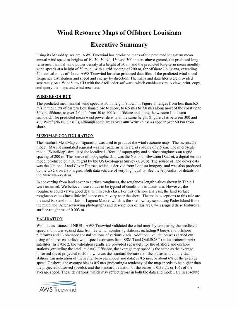
The predicted mean annual wind speed at 50 m height (shown in Figure 1) ranges from less than 6.5 m/s in the inlets of eastern Louisiana close to shore, to 6.5 m/s to 7.0 m/s along most of the coast up to 50 km offshore, to over 7.0 m/s from 50 to 100 km offshore and along the western Louisiana seaboard. The predicted mean wind power density at the same height (Figure 2) is between 300 and 400 W/m2 (NREL class 3), although some areas over 400 W/m2 (class 4) appear over 50 km from shore.

MESOMAP CONFIGURATION

The standard MesoMap configuration was used to produce the wind resource maps. The mesoscale model (MASS) simulated regional weather patterns with a grid spacing of 2.5 km. The microscale model (WindMap) simulated the localized effects of topography and surface roughness on a grid spacing of 200 m. The source of topographic data was the National Elevation Dataset, a digital terrain model produced on a 30 m grid by the US Geological Survey (USGS). The source of land cover data was the National Land Cover Dataset, which is derived from Landsat imagery, and was also produced by the USGS on a 30 m grid. Both data sets are of very high quality. See the Appendix for details on the MesoMap system.

In converting from land cover to surface roughness, the roughness length values shown in Table 1 were assumed. We believe these values to be typical of conditions in Louisiana. However, the roughness could vary a good deal within each class. For this offshore analysis, the land surface roughness values have little influence except very near the shore. The main exceptions to this rule are the sand bars and mud flats of Laguna Madre, which is the shallow bay separating Padre Island from the mainland. After reviewing photographs and descriptions of this area, we assigned these features a surface roughness of 0.003 m.

VALIDATION

With the assistance of NREL, AWS Truewind validated the wind maps by comparing the predicted speed and power against data from 22 wind monitoring stations, including 9 buoys and offshore platforms and 13 on-shore coastal stations of various kinds. Additional validation was carried out using offshore sea surface wind speed estimates from SSM/I and QuikSCAT (radio scatterometer) satellites. In Table 2, the validation results are provided separately for the offshore and onshore stations (excluding the satellite data). Offshore, the average map speed is the same as the average observed speed projected to 50 m, whereas the standard deviation of the biases at the individual stations (an indication of the scatter between model and data) is 0.5 m/s, or about 6% of the average speed. Onshore, the average bias is 0.5 m/s (indicating a tendency of the map speeds to be higher than the projected observed speeds), and the standard deviation of the biases is 0.5 m/s, or 10% of the average speed. These deviations, which may reflect errors in both the data and model, are in absolute

2

terms within the normal range for the MesoMap system. However, the relative deviations onshore are somewhat greater than usual. We believe this is mainly because the relatively low average wind speed makes the errors proportionately larger. It should be noted that there is considerable uncertainty in the projected 50 m speeds both onshore and offshore because most of the towers are much shorter than 50 m and there are few direct measurements of wind shear. We estimate the uncertainty in the projected 50 m speeds to be 5-10%.

As a result of the validation, we increased the predicted speed and power by 4% and 12%, respectively, off the eastern Louisiana coast. The map speeds in Table 2 include these adjustments.

It should be stressed that the mean wind speed at any particular location may depart significantly from the predicted values. While land cover and topography have no bearing offshore, other factors may cause errors. See the Appendix for guidelines on using the wind maps.

Table 1. Range of Surface Roughness Values

for Leading Land Cover Types

Description Roughness (m)

Coniferous Forest 1.125 Deciduous Forest 0.90 Shrubland / Transitional 0.07 & 0.15 Cropland / Grassland 0.05 & 0.03 Wetland 0.20 & 0.66 Bare rock / Soil 0.01 Mudflats and Sand Bars 0.003 Airports 0.02 Built-up Environment 0.55 Water Charnock relation*

*The Charnock relation relates the roughness of water bodies to the square of the friction velocity.

3

Table 2. Observed and Predicted Mean Wind Speeds

Name Type* Lat. Long. Elevation

(m)

Obs. Height

(m)

Projected 50 m

Speed (m/s)

Map 50 m

Speed (m/s)

Bias (m/s)

ONSHORE Boothville City 29.342 89.413 0 6.1 5.4 5.5 0.1 Cameron Heliport Airport 29.777 93.300 1 10.0 4.9 6.1 1.2 Fourchon Airport 29.112 90.208 2 10.0 5.7 5.6 -0.1 Golden Tri Airport 29.269 89.353 2 10.0 4.0 5.7 1.7 Grand Isle Airport 29.255 89.966 2 10.0 5.3 5.9 0.6 Grand Isle CG 29.266 89.957 2 8.0 6.0 6.1 0.1 Grand Isle CMAN 29.267 89.957 0 15.8 5.7 6.1 0.4 Intracoastal City Airport 29.825 92.134 5 10.0 4.3 5.6 1.3 Marine Center LUMCON 29.254 90.661 1 13.2 4.9 5.7 0.8 Southwest Pass CG 28.906 89.429 1 18.5 6.8 6.8 0.0 Southwest Pass CMAN 28.905 89.428 0 30.5 6.5 6.8 0.3 Tambour Bay LUMCON 29.188 90.665 0 10.0 6.0 6.4 0.4 Terrebonne Bay LUMCON 29.167 90.583 0 13.9 6.7 6.8 0.1 Average 5.6 6.1 0.5

Standard Deviation 0.5

(10%)OFFSHORE Buoy 42007 NDBC 30.090 88.769 0 5.0 7.3 6.7 -0.6 Buoy 42040 NDBC 29.184 88.213 0 5.0 7.2 7.1 -0.1 Buoy 42067 NDBC 30.044 88.658 0 5.0 7.1 6.7 -0.4 Buoy 42011 NDBC 29.600 93.500 0 15.0 7.0 7.1 0.1 Buoy 42010 NDBC 29.700 93.400 0 15.0 6.4 7.0 0.6 Isle Derniers LSU 29.053 90.533 0 19.2 6.8 6.7 -0.1 Marsh Island LSU 29.440 92.061 1 23.4 6.3 6.9 0.6 Ship Island Pass LSU 30.267 89.017 0 11.0 6.8 6.4 -0.4 South Timbalier LSU 28.867 90.483 0 40.4 6.7 6.8 0.1 Average 6.8 6.8 0.0

Standard Deviation 0.4

(6%) *Abbreviations: CG = Coast Guard; CMAN = Coastal Marine Automated Network; LUMCON = Louisiana Universities Marine Consortium; LSU = Louisiana State University; NDBC = National Data Buoy Center.

4

Figure 1. Mean Annual Wind Speed for Offshore Region of Louisiana at 50 m

5

Figure 2. Mean Annual Wind Power Density for Offshore Region of Louisiana at 50 m

6

Appendix

The MesoMap System The MesoMap system was developed by AWS Truewind to map the wind resources of large regions at a high level of detail and with good accuracy. It accomplishes this by combining a state-of-the-art numerical weather model for simulating regional (mesoscale) weather patterns with a wind flow model responsive to local (microscale) terrain and surface conditions. Using weather data collected from weather balloons, satellites, and meteorological stations as its main inputs, MesoMap does not require wind data to make reasonably accurate predictions. However such data are still required to confirm the wind resource at any particular location before major investments are made in a wind project. In the past five years, MesoMap has been applied in over 30 countries on four continents. In North America alone, MesoMap has been used to map over 30 US states and several provinces of Canada and states of Mexico. The typical error margin is 5-7%, depending on the complexity of the terrain and the size of the region.

DESCRIPTION

The MesoMap system has three main components: models, databases, and computer systems. These components are described below.

Models

At the core of the MesoMap system is MASS (Mesoscale Atmospheric Simulation System), a numerical weather model that has been developed over the past 20 years by AWS Truewind’s partner MESO, Inc., both as a research tool and to provide commercial weather forecasting services.1 MASS simulates the fundamental physics of the atmosphere including conservation of mass, momentum, and energy, as well as the moisture phases, and it contains a turbulent kinetic energy module that accounts for the effects of viscosity and thermal stability on wind shear. A dynamic model, MASS simulates the evolution of atmospheric conditions in time steps as short as a few seconds. This creates great computational demands, especially when running at high resolution. Hence MASS is usually coupled to a simpler but much faster program, WindMap, a mass-conserving wind flow model developed by AWS Truewind.2 Depending on the size and complexity of the region and requirements of the client, WindMap is used to improve the spatial resolution of the MASS simulations to account for the local effects of terrain and surface roughness variations.

Data Sources

MASS uses a variety of online, global, geophysical and meteorological databases. The main meteorological inputs are reanalysis data, rawinsonde data, and land surface measurements. The reanalysis database – the most important – is a gridded historical data set produced by the US National Centers for Environmental Prediction (NCEP) and National Center for Atmospheric Research (NCAR).3 The data provide a snapshot of atmospheric conditions around the word at all levels of the atmosphere in intervals of six hours. Along with rawinsonde and surface data, the

1 Manobianco, J., J. W. Zack and G.E. Taylor, 1996: Workstation-based real-time mesoscale modeling designed for weather support to operations at the Kennedy Space Center and Cape Canaveral Air Station. Bull. Amer. Meteor. Soc., 77, 653-672. Embedded equations are described in Zack, J., et al., 1995: MASS Version 5.6 Reference Manual. MESO, Inc., Troy, NY. 2 Brower, M.C., 1999: Validation of the WindMap Model and Development of MesoMap, Proc. of Windpower 1999, American Wind Energy Association, Washington, DC. 3 Robert Kistler et al., The NCEP/NCAR Reanalysis, Bulletin of the American Meteorological Society (2001).

7

reanalysis data establish the initial conditions as well as lateral boundary conditions for the MASS runs. The MASS model itself determines the evolution of atmospheric conditions within the region based on the interactions among different elements in the atmosphere and between the atmosphere and the surface. The reanalysis data are on a relatively coarse grid (about 210 km spacing). To avoid generating noise at the boundaries that can result from large jumps in grid cell size, MASS is run in several nested grids of successfully finer mesh size, each taking as input the output of the previous nest, until the desired grid scale is reached. The outermost grid typically extends several thousand kilometers.

The main geophysical inputs are elevation, land cover, vegetation greenness (normalized differential vegetation index, or NDVI), soil moisture, and sea-surface temperatures. The elevation data used by MASS are from the Shuttle Radar Topographical Mission 30 Arc-Second Data Set (SRTM30), which was produced in an international project spearheaded by the National Geospatial-Intelligence Agency (NGA) and the National Aeronautics and Space Administration (NASA).4 The land cover data are from the satellite-based Moderate Resolution Imaging Spectro-radiometer (MODIS) data set.5 The NDVI data were derived from a predecessor of MODIS, the satellite-based Advanced Very High Resolution Radiometer (AVHRR).6 The nominal spatial resolution of all of these data sets is 1 km.

Maps of much higher resolution than 1 km can be produced either by MASS or by WindMap if the necessary topographical and land cover data are available. In the past year, 3 arc-second SRTM data have been released for most of the world except the polar regions. These data provide highly accurate elevations on a 90 m horizontal grid (30 m in the United States). A data set called GeoCover, from EarthSat, offers high-quality land cover classifications on a 28 m grid for most of the world.7 The WindMap model automatically adjusts for differences in elevation and surface roughness between the mesoscale and microscale.

Computer and Storage Systems

The MesoMap system requires a very powerful set of computers and storage systems to produce detailed wind resource maps in a reasonable amount of time. To meet this need AWS Truewind has created a distributed processing network consisting of about 130 Pentium II processors and 10 terabytes of hard disk storage. Since each day simulated by a processor is entirely independent of other days, a project can be run on this system up to 130 times faster than would be possible with any single processor. To put it another way, a typical MesoMap project that would take two years to run on a single processor can be completed in about a week.

THE MAPPING PROCESS

The MesoMap system creates a wind resource map in several steps. First, the MASS model simulates weather conditions over 366 days selected from a 15-year period. The days are chosen through a stratified random sampling scheme so that each month and season is represented equally in the sample; only the year is randomized. Each simulation generates wind and other weather variables (including temperature, pressure, moisture, turbulent kinetic energy, and heat flux) in three dimensions throughout the model domain, and the information is stored at hourly intervals. When the runs are finished, the results are summarized in files, which are then input into the WindMap program for the final mapping stage. The two main products are usually (1) color-coded maps of mean wind speed and power density at various heights above ground and (2) data files containing wind speed and direction frequency distribution parameters.

4For more information, see http://www2.jpl.nasa.gov/srtm/. 5See http://edcdaac.usgs.gov/modis/mod12q1.asp. 6See http://edcwww.cr.usgs.gov/products/landcover/glcc.html. 7See http://www.mdafederal.com/geocover/geocoverlc.

8

Once completed, the maps and data can be compared with land and ocean surface wind measurements, and if significant discrepancies are observed, the wind maps can be adjusted. The most common sources of validation data are tall towers instrumented for wind energy assessment and standard meteorological stations. The validation is usually carried out in the following steps:

1. Station locations are verified and adjusted, if necessary, by comparing the quoted elevations and station descriptions against the elevation and land cover maps. Where there are obvious errors in position, the stations are moved to the nearest point with the correct elevation and surface characteristics.

2. The observed mean speed and power are adjusted to the long-term climate norm and then extrapolated to the map height using the power law. Often, for the tall towers, little or no extrapolation is needed. Where multi-level data are available, the observed mean wind shear exponent is used. Where measurements were taken at a single height, the wind shear is estimated from available information concerning the station location and surroundings.

3. The predicted and measured/extrapolated speeds are compared, and the map bias (map speed minus measured/extrapolated speed) is calculated for each point. If there are enough towers, the mean bias and standard deviation of the biases is calculated. (It is important to note that the bias and standard deviation may reflect errors in the data as well as the map.)

4. If we detect a pattern of bias, the maps are adjusted to reduce or eliminate the discrepancy.

The MesoMap system has been validated in this fashion using data from well over 1000 stations worldwide. We have found the typical standard error, after accounting for uncertainty in the data, to be 5-7% of the mean speed at a height of 50 m.

FACTORS AFFECTING ACCURACY

In our experience, the most important sources of error in the wind resource estimates produced by MesoMap are the following:

• Finite grid scale of the simulations

• Errors in assumed surface properties such as roughness

• Errors in the topographical and land cover data bases

The finite grid scale of the simulations results in a smoothing of terrain features such as mountains and valleys. For example, a mountain ridge that is 2000 m above sea level may appear to the model to be only 1600 m high. Where the flow is forced over the terrain, this smoothing can result in an underestimation of the mean wind speed or power at the ridge top. Where the mountains block the flow, on the other hand, the smoothing can result in an overestimation of the resource, as the model understates the blocking effect. The problem of finite grid scale can be solved by increasing the spatial resolution of the simulations, but at a cost in computer processing and storage.

While topographic data are usually reliable, errors in the size and location of terrain features nonetheless occur from time to time. Errors in the land cover data are more common, and usually result from the misclassification of aerial or satellite imagery. Wherever possible, AWS Truewind uses the most accurate and detailed land cover databases.

Assuming the land cover types are correctly identified, there remains uncertainty in the surface properties that should be assigned to each type, and especially the vegetation height and roughness. A forest, for example, may consist of a variety of trees of varying heights and density, leaf characteristics, and other features affecting surface roughness. An area designated as cropland may be devoid of trees, or it may be broken up into fields separated by windbreaks. Uncertainties such as these can be resolved only by visiting the region and verifying firsthand the land cover data. However this is not practical when (as in most MesoMap projects) the area being mapped is large.

9

GUIDELINES FOR INTERPRETING AND USING THE MAPS

The following are guidelines for interpreting and adjusting the wind speed estimates in the maps. They are most easily used in conjunction with the WindView ArcReader CD. The CD allows users to obtain the “exact” wind speed value at any point, and provides the elevation and surface roughness data used by the model, which are needed to apply the adjustment formulas given below.

1. The maps assume that all locations are free of obstacles that could disrupt or impede the wind flow. “Obstacle” does not apply to trees if they are common to the landscape, since their effects are already accounted for in the predicted speed. However, a large outcropping of rock or a building would pose an obstacle, as would a nearby shelterbelt of trees or a building in an otherwise open landscape. As a rule of thumb, the effect of such obstacles extends to a height of about twice the obstacle height and to a distance downwind of 10-20 times the obstacle height.

2. Generally speaking, points that lie above the average elevation within a grid cell will be somewhat windier than points that lie below it. A rule of thumb is that every 100 m increase in elevation will raise the mean speed by about 0.5-1 m/s. This formula is most applicable to small, isolated hills or ridges in flat terrain.

3. The mean wind speed can be affected by the surface roughness up to several kilometers away. If the roughness is much lower than that assumed by the model, the mean wind speed may be higher, and vice-versa. Typical values of roughness range from 0.01 m in open, flat ground without significant trees or shrubs, to 0.1 m in land with widely scattered trees and small buildings, to 1 m or more for built-up or forested areas. These values are only indirectly related to the size of the vegetation and buildings.

The following equation provides an approximate speed adjustment for differences in surface roughness in the direction of the wind:

−

−

×

−

−

≈

02

02

01

01

1

2

300log

log

log

300log

zd

zdh

zdh

zd

vv

v1 and v2 are the original and adjusted wind speeds at height h (in meters above ground level); z01 and z02 are the model and actual surface roughness values (in meters); and d1 and d2 are the corresponding displacement heights. (This equation assumes the wind is unaffected by roughness changes above a height of 300 m. It is, in other words, intended to deal only with differences in roughness on a local scale.)

As an example, suppose the surface roughness assumed by the model was 0.2 m, and the displacement 2 m, whereas the true roughness is 0.75 m and displacement 7.5 m. For h = 50 m, the above formula gives

90.0

75.05.7300log

75.05.750log

2.0250log

2.02300log

1

2 =

−

−

×

−

−

≈vv

This shows that the predicted wind speed should be reduced by about 10%.

This formula assumes that the wind is in equilibrium with the new surface roughness above the height of interest (in this case 50 m). When going from high roughness to low roughness (such as from forested to open land), the clearing should be at least 1000 m wide for the benefit of the lower roughness to be fully realized. However, when going from low to high roughness, the

10

reduction in wind speed may be felt over a much shorter distance. For this and other reasons, the formula should be applied with care.