Wind Speed Ensemble Forecasting Based on Deep LearningUsing Adaptive Dynamic Optimization Algorithm

Author

Ibrahim, A, Mirjalili, S, El-Said, M, Ghoneim, SSM, ALHARTHI, M, Ibrahim, TF, El-kenawy,ESM

Published

2021

Journal Title

IEEE Access

Version

Version of Record (VoR)

DOI

https://doi.org/10.1109/ACCESS.2021.3111408

Copyright Statement

© The Author(s) 2021. This is an Open Access article distributed under the terms of theCreative Commons Attribution 4.0 International License, which permits unrestricted use,distribution, and reproduction in any medium, provided the original work is properly cited.

Downloaded from

http://hdl.handle.net/10072/408377

Griffith Research Online

https://research-repository.griffith.edu.au

Received August 13, 2021, accepted September 4, 2021, date of publication September 9, 2021,date of current version September 17, 2021.

Digital Object Identifier 10.1109/ACCESS.2021.3111408

Wind Speed Ensemble Forecasting Based onDeep Learning Using Adaptive DynamicOptimization AlgorithmABDELHAMEED IBRAHIM 1, (Member, IEEE),SEYEDALI MIRJALILI 2,3, (Senior Member, IEEE), M. EL-SAID 4,5,SHERIF S. M. GHONEIM 6, (Senior Member, IEEE), MOSLEH M. AL-HARTHI 6,TAREK F. IBRAHIM7,8, AND EL-SAYED M. EL-KENAWY 9,10, (Member, IEEE)1Computer Engineering and Control Systems Department, Faculty of Engineering, Mansoura University, Mansoura 35516, Egypt2Centre for Artificial Intelligence Research and Optimization, Torrens University Australia, Fortitude Valley, QLD 4006, Australia3Yonsei Frontier Lab, Yonsei University, Seoul 03722, South Korea4Electrical Engineering Department, Faculty of Engineering, Mansoura University, Mansoura 35516, Egypt5Delta Higher Institute of Engineering and Technology (DHIET), Mansoura 35111, Egypt6Electrical Engineering Department, College of Engineering, Taif University, Taif 21944, Saudi Arabia7Department of Mathematics, Faculty of Sciences and Arts (Mahayel), King Khalid University, Abha 62529, Saudi Arabia8Department of Mathematics, Faculty of Science, Mansoura University, Mansoura 35516, Egypt9Department of Communications and Electronics, Delta Higher Institute of Engineering and Technology (DHIET), Mansoura 35111, Egypt10Faculty of Artificial Intelligence, Delta University for Science and Technology, Mansoura 35712, Egypt

Corresponding authors: El-Sayed M. El-Kenawy (skenawy@ieee.org) and Abdelhameed Ibrahim (afai79@mans.edu.eg)

This work was supported by Taif University Researchers Supporting Project through Taif University, Taif, Saudi Arabia, under GrantTURSP-2020/122.

ABSTRACT The development and deployment of an effective wind speed forecasting technology canimprove the safety and stability of power systems with significant wind penetration. Due to the wind’sunpredictable and unstable qualities, accurate forecasting of wind speed and power is extremely challenging.Several algorithms were proposed for this purpose to improve the level of forecasting reliability. TheLong Short-Term Memory (LSTM) network is a common method for making predictions based on timeseries data. This paper proposed a machine learning algorithm, called Adaptive Dynamic Particle SwarmAlgorithm (AD-PSO) combined with Guided Whale Optimization Algorithm (Guided WOA), for windspeed ensemble forecasting. The AD-PSO-Guided WOA algorithm selects the optimal hyperparametersvalue of the LSTM deep learning model for forecasting of wind speed. In experiments, a wind powerforecasting dataset is employed to predict hourly power generation up to forty-eight hours ahead at sevenwind farms. This case study is taken from the Kaggle Global Energy Forecasting Competition 2012 in windforecasting. The results demonstrated that the AD-PSO-Guided WOA algorithm provides high accuracyand outperforms several comparative optimization and deep learning algorithms. Different tests’ statisticalanalysis, includingWilcoxon’s rank-sum and one-way analysis of variance (ANOVA), confirms the accuracyof the presented algorithm.

INDEX TERMS Artificial intelligence, machine learning, optimization, forecasting, guided whaleoptimization algorithm.

I. INTRODUCTIONDue to the intermittence and unpredictability of wind power,the increasing penetration of wind power into power gridsmight significantly impact the safe functioning of power sys-tems and power quality because the amount of wind energy

The associate editor coordinating the review of this manuscript and

approving it for publication was Dipankar Deb .

generated is proportional to the wind speed. As a result,the development and deployment of an effective wind speedforecasting technology can be able to improve the safety andstability of power systems with significant wind penetration.Wind energy is one of the essential low-carbon energy tech-nologies. It can deliver a long-term energy supply and servesas a core component for micro-grids as part of intelligent gridarchitecture [1].

VOLUME 9, 2021 This work is licensed under a Creative Commons Attribution 4.0 License. For more information, see https://creativecommons.org/licenses/by/4.0/ 125787

A. Ibrahim et al.: Wind Speed Ensemble Forecasting Based on Deep Learning

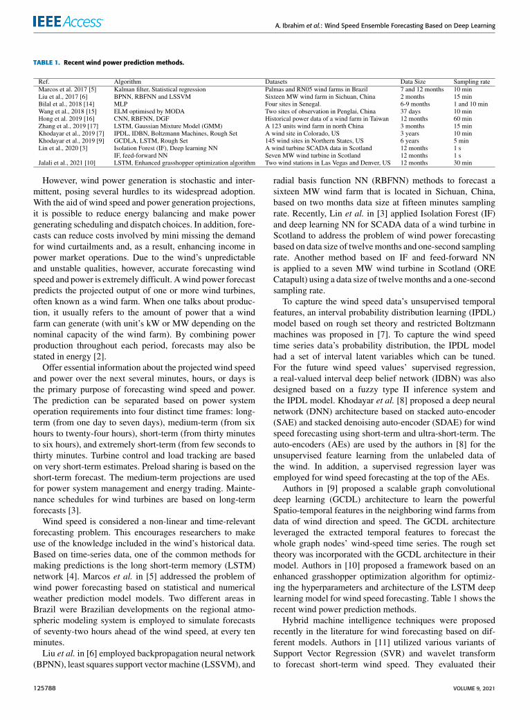
TABLE 1. Recent wind power prediction methods.

However, wind power generation is stochastic and inter-mittent, posing several hurdles to its widespread adoption.With the aid of wind speed and power generation projections,it is possible to reduce energy balancing and make powergenerating scheduling and dispatch choices. In addition, fore-casts can reduce costs involved by mini missing the demandfor wind curtailments and, as a result, enhancing income inpower market operations. Due to the wind’s unpredictableand unstable qualities, however, accurate forecasting windspeed and power is extremely difficult. Awind power forecastpredicts the projected output of one or more wind turbines,often known as a wind farm. When one talks about produc-tion, it usually refers to the amount of power that a windfarm can generate (with unit’s kW or MW depending on thenominal capacity of the wind farm). By combining powerproduction throughout each period, forecasts may also bestated in energy [2].

Offer essential information about the projected wind speedand power over the next several minutes, hours, or days isthe primary purpose of forecasting wind speed and power.The prediction can be separated based on power systemoperation requirements into four distinct time frames: long-term (from one day to seven days), medium-term (from sixhours to twenty-four hours), short-term (from thirty minutesto six hours), and extremely short-term (from few seconds tothirty minutes. Turbine control and load tracking are basedon very short-term estimates. Preload sharing is based on theshort-term forecast. The medium-term projections are usedfor power system management and energy trading. Mainte-nance schedules for wind turbines are based on long-termforecasts [3].

Wind speed is considered a non-linear and time-relevantforecasting problem. This encourages researchers to makeuse of the knowledge included in the wind’s historical data.Based on time-series data, one of the common methods formaking predictions is the long short-term memory (LSTM)network [4]. Marcos et al. in [5] addressed the problem ofwind power forecasting based on statistical and numericalweather prediction model models. Two different areas inBrazil were Brazilian developments on the regional atmo-spheric modeling system is employed to simulate forecastsof seventy-two hours ahead of the wind speed, at every tenminutes.

Liu et al. in [6] employed backpropagation neural network(BPNN), least squares support vector machine (LSSVM), and

radial basis function NN (RBFNN) methods to forecast asixteen MW wind farm that is located in Sichuan, China,based on two months data size at fifteen minutes samplingrate. Recently, Lin et al. in [3] applied Isolation Forest (IF)and deep learning NN for SCADA data of a wind turbine inScotland to address the problem of wind power forecastingbased on data size of twelvemonths and one-second samplingrate. Another method based on IF and feed-forward NNis applied to a seven MW wind turbine in Scotland (ORECatapult) using a data size of twelvemonths and a one-secondsampling rate.

To capture the wind speed data’s unsupervised temporalfeatures, an interval probability distribution learning (IPDL)model based on rough set theory and restricted Boltzmannmachines was proposed in [7]. To capture the wind speedtime series data’s probability distribution, the IPDL modelhad a set of interval latent variables which can be tuned.For the future wind speed values’ supervised regression,a real-valued interval deep belief network (IDBN) was alsodesigned based on a fuzzy type II inference system andthe IPDL model. Khodayar et al. [8] proposed a deep neuralnetwork (DNN) architecture based on stacked auto-encoder(SAE) and stacked denoising auto-encoder (SDAE) for windspeed forecasting using short-term and ultra-short-term. Theauto-encoders (AEs) are used by the authors in [8] for theunsupervised feature learning from the unlabeled data ofthe wind. In addition, a supervised regression layer wasemployed for wind speed forecasting at the top of the AEs.

Authors in [9] proposed a scalable graph convolutionaldeep learning (GCDL) architecture to learn the powerfulSpatio-temporal features in the neighboring wind farms fromdata of wind direction and speed. The GCDL architectureleveraged the extracted temporal features to forecast thewhole graph nodes’ wind-speed time series. The rough settheory was incorporated with the GCDL architecture in theirmodel. Authors in [10] proposed a framework based on anenhanced grasshopper optimization algorithm for optimiz-ing the hyperparameters and architecture of the LSTM deeplearning model for wind speed forecasting. Table 1 shows therecent wind power prediction methods.

Hybrid machine intelligence techniques were proposedrecently in the literature for wind forecasting based on dif-ferent models. Authors in [11] utilized various variants ofSupport Vector Regression (SVR) and wavelet transformto forecast short-term wind speed. They evaluated their

125788 VOLUME 9, 2021

A. Ibrahim et al.: Wind Speed Ensemble Forecasting Based on Deep Learning

proposed techniques using various performance indices to getthe best regressor for wind forecasting applications. A hybridtechnique was presented in [12] using learning algorithmssuch as Twin SVR (TSVR), Convolutional neural networks(CNN), and random forest, in addition to, discrete wavelettransform (DWT) for wind forecasting. The extracted featuresfrom wind speed in their work were enhanced based on thewavelet transform. Another hybrid technique was proposedfor the anomaly detection problem for wind turbine gearboxin [13] using adaptive threshold and twin SVM (TWSVM)methods.

In this work, a dataset of wind power forecasting istested as a case study from Kaggle Global Energy Fore-casting Competition 2012-Wind Forecasting for predictinghourly power generation up to forty-eight hours ahead atseven different wind farms. A proposed adaptive dynamicparticle swarm algorithm (AD-PSO) with a guided whaleoptimization algorithm (Guided WOA) improves the fore-casting performance by enhancing the parameters of theLSTM classificationmethod. The proposed AD-PSO-GuidedWOA algorithm selects the value of the optimal hyperpa-rameter of the LSTM deep learning model for forecastingpurposes of wind speed. A binary-based AD-PSO-GuidedWOA algorithm is used for the feature selection problemfrom the wind power forecasting dataset. The evaluation ofthe binary AD-PSO-Guided WOA algorithm is presentedcompared to Grey Wolf Optimizer (GWO) [18], ParticleSwarm Optimization (PSO) [19], Stochastic Fractal Search(SFS) [20], WOA [21], [22], Genetic Algorithm (GA) [23],and Firefly Algorithm (FA) [24]. The optimized ensemblemethod based on the proposed algorithm is tested on thedataset. The results of this scenario are compared with Neu-ral Networks (NN), Random Forest (RF), LSTM, Averageensemble, and k-Nearest Neighbors (k-NN) ensemble-basedmethods.

The AD-PSO-Guided WOA algorithm ensemble modelis compared with other optimization techniques includ-ing PSO [19], WOA [22], GA [23], GWO [18], HarrisHawks Optimization (HHO) [25], [26], Slime Mould Algo-rithm (SMA) [27], Marine Predators Algorithm (MPA) [28],and Chimp Optimization Algorithm (ChOA) [29]. TheAD-PSO-Guided WOA algorithm ensemble model is alsocompared with other deep learning techniques includingTime delay neural network (TDNN) [30], Deep NeuralNetworks (DNN) [31], Stacked Denoising Autoencoder(SAE) [32], and Bidirectional Recurrent Neural Networks(BRNN) [33]. The statistical analysis of different tests isperformed to confirm the accuracy of the algorithm, includinga one-way analysis of variance (ANOVA) and Wilcoxon’srank-sum. The contributions of this work are summarized asfollows.• An adaptive dynamic PSO with guided WOA algorithm(AD-PSO-Guided WOA) is suggested.

• A binary AD-PSO-Guided WOA algorithm is testedfor the feature selection problem using the wind powerforecasting dataset.

• Tests of one-sample t-test and ANOVA are used toevaluate the binary AD-PSO-Guided WOA algorithm’sstatistical difference.

• To improve the wind power forecasting accuracy,an optimized ensemble method using the AD-PSO-Guided WOA algorithm is proposed.

• Wilcoxon’s rank-sum and ANOVA tests are used forevaluating the proposed optimizing ensemble method’sstatistical difference.

• The current work’s importance is applying a newoptimization algorithm to enhance LSTM classifierparameters.

• The proposed algorithms can be generalized and testedfor other datasets.

II. PRELIMINARIESA. MACHINE LEARNING1) NEURAL NETWORKS (NNs)Artificial neural networks (ANNs) are a type of predictionmodel and classification approach. ANN is used to simulatecomplicated relationships of finding data patterns or cause-and-effect variable sets. Transient detection, approximation,time-series prediction, and pattern recognition are just afew of the disciplines they may use. ANN is considered aninformation processing pattern that functions similarly to thehuman brain. This information processing system compriseshighly linked processing pieces called neurons that worktogether to solve issues in tandem. When formulating analgorithmic solution, a neural network comes in handy andwhere it is necessary to extract the structure from existingdata [34].

A Multilayer perceptron (MLP) has input, output and onehidden layer. The weighted sum for the node output value iscomputed as follows [35].

Sj =n∑i=1

wijIi + βj (1)

where Ii represents an input variable i, the weight of connec-tion between neuron j and input Ii is represented as wij. Theβj parameter is a bias value. Based on using of the sigmoidactivation function, the node j output is calculated as

fj(Sj) =1

1+ e−Sj(2)

where the value of fj(Sj) is then used to get the network outputas follows.

yk =m∑j=1

wjk fj(Sj)+ βk (3)

where the weights between output node k and neuron j in thehidden layer is defined aswjk and βk indicates the output layerbias value.

2) RANDOM FOREST (RF)As a method based on statistical learning theory, ran-dom forests provide several advantages, including fewer

VOLUME 9, 2021 125789

A. Ibrahim et al.: Wind Speed Ensemble Forecasting Based on Deep Learning

configurable parameters, higher prediction precision, andimproved generalization ability. It extracts numerous sam-ples from the original sample using the bootstrap samplingapproach, builds decision tree modeling based on each boot-strap sample, combines the predictions of multiple decisiontrees, and uses a voting mechanism to determine the outcome.

For the RF training algorithm, the regression/classificationtree fb is trained based on Xb and Yb training examples forX = x1, . . . , xn and Y = y1, . . . , yn. For B times, let b =1, . . . ,B. After the process of training, the unseen samplespredictions x ′ is calculated by averaging all the predictionsof individual regression trees on x ′ as in equation 4.

f =1B

B∑b=1

fb(x ′) (4)

3) K-NEAREST NEIGHBORS (K-NN)The model’s interpretability. The findings of the predictionalgorithm using the k-nearest neighbor’s technique are basedon the previous events that are the most like the current statebased on a given distance metric. A simple average of theoutput values of the k nearest neighbors, or any weightedaveraging, is used to make predictions. Thus, experts cananalyze the findings of the k-nearest neighbor’s method. Theobject’s predictable variable in the k-NN numerical predic-tion this number is the average of its k closest neighbors’values. The k-NN method is one of the basic and the mostpowerful machine learning algorithms.

The k-NN model employs a similarity measure, Euclideandistance, to compare the data. Between xtrain as training dataand xtest as testing data, calculations of the Euclidean distanceare based on the following equation.

D(xtrain,i, xtest,i

)=

√√√√ k∑i=1

(xtrain,i − xtest,i)2 (5)

To predict the output variables, k-NN determines k trainingdata close to testing data. For unknown testing data to bepredicted, the k training data output value is determined tobe the nearest neighbours. The following formula is appliedfor predicting the testing data.

y =k∑j=1

wjyj (6)

where the jth neighbor weight is indicated as wj and it isadjusted by the observed data, for wj = j/n, for n indicatesnumber of training data. This model can be used as a k-NNtime series model.

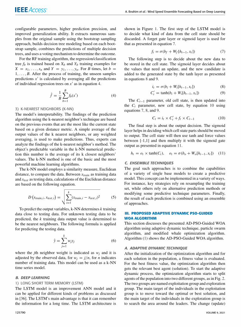
B. DEEP LEARNING1) LONG SHORT TERM MEMORY (LSTM)The LSTM model is an improvement ANN model and itcan be applied for different kinds of problems as discussedin [36]. The LSTM’s main advantage is that it can rememberthe information for a long time. The LSTM architecture is

shown in Figure 1. The first step of the LSTM model isto decide what kind of data from the cell state should bediscarded. A forget gate layer or sigmoid layer is used forthat as presented in equation 7.

ft = σ (bf +Wf [ht−1, xt ]) (7)

The following step is to decide about the new data tobe stored in the cell state. The sigmoid layer decides aboutthe values that need an update, and the new candidate isadded to the generated state by the tanh layer as presentedin equations 8 and 9.

it = σ (bi +Wi[ht−1, xt ]) (8)

C ′t = tanh(bi +Wi[ht−1, xt ]) (9)

The Ct−1 parameter, old cell state, is then updated intothe Ct parameter, new cell state, by equation 10 usingequations 7, 8, and 9.

Ct = it × C ′t + ft × Ct−1 (10)

The final step is about the output decision. The sigmoidlayer helps in deciding which cell state parts should be movedto output. The cell state will then use tanh and force valuesbetween [-1,1] and then multiply it with the sigmoid gateoutput as presented in equation 11.

ht = ot × tanh(Ct ), ot = σ (bo +Wo[ht−1, xt ]) (11)

C. ENSEMBLE TECHNIQUESThe goal such approaches is to combine the capabilitiesof a variety of single base models to create a predictivemodel. This concept can be implemented in a variety of ways.For instance, key strategies rely on resampling the trainingset, while others rely on alternative prediction methods ormodifying some predictive technique parameters. Finally,the result of each prediction is combined using an ensembleof approaches.

III. PROPOSED ADAPTIVE DYNAMIC PSO-GUIDEDWOA ALGORITHMThis section discusses the presented AD-PSO-Guided WOAalgorithm using adaptive dynamic technique, particle swarmalgorithm, and modified whale optimization algorithm.Algorithm (1) shows the AD-PSO-Guided WOA algorithm.

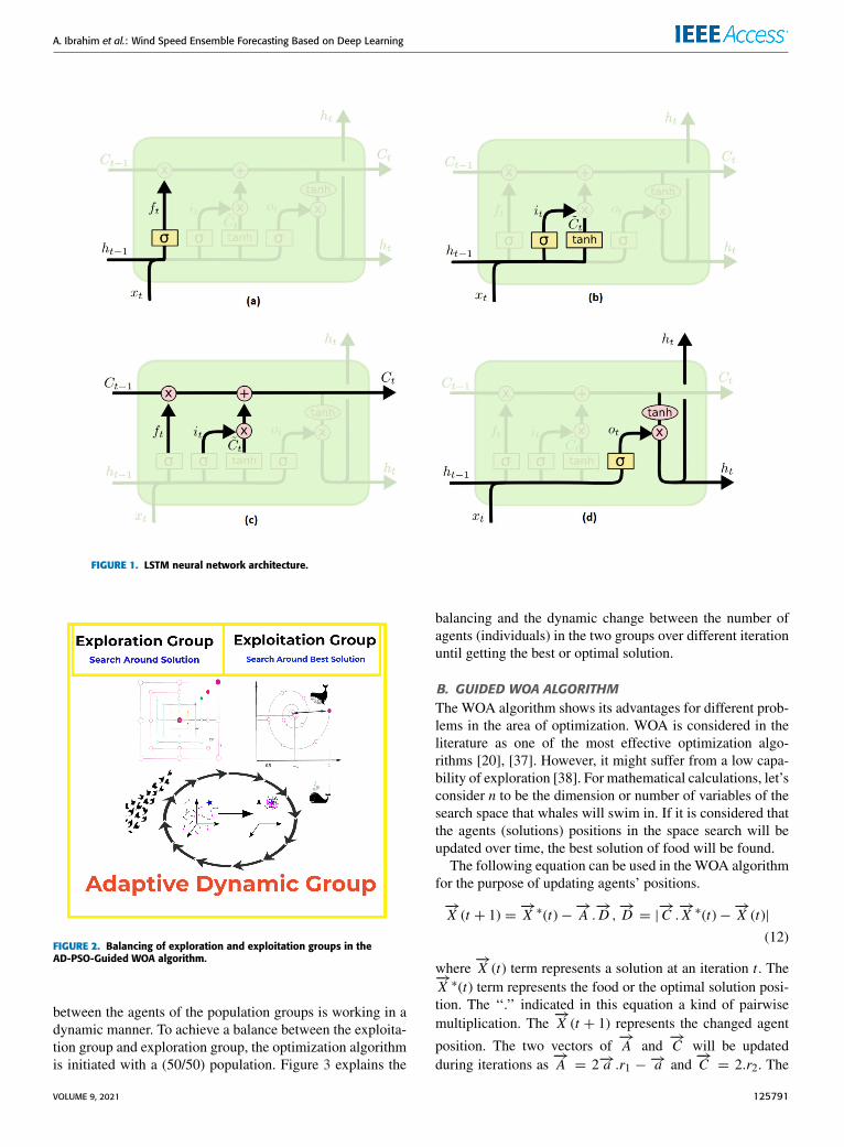
A. ADAPTIVE DYNAMIC TECHNIQUEAfter the initialization of the optimization algorithm and foreach solution in the population, a fitness value is evaluated.For the best fitness value, the optimization algorithm thengets the relevant best agent (solution). To start the adaptivedynamic process, the optimization algorithm starts to splitagents of the population into two different groups, as in Fig. 2.The two groups are named exploitation group and explorationgroup. The main target of the individuals in the exploitationgroup is to move toward the optimal or best solution, andthe main target of the individuals in the exploration group isto search the area around the leaders. The change (update)

125790 VOLUME 9, 2021

A. Ibrahim et al.: Wind Speed Ensemble Forecasting Based on Deep Learning

FIGURE 1. LSTM neural network architecture.

FIGURE 2. Balancing of exploration and exploitation groups in theAD-PSO-Guided WOA algorithm.

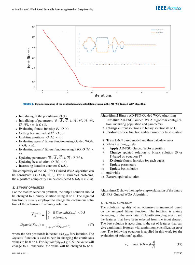
between the agents of the population groups is working in adynamic manner. To achieve a balance between the exploita-tion group and exploration group, the optimization algorithmis initiated with a (50/50) population. Figure 3 explains the

balancing and the dynamic change between the number ofagents (individuals) in the two groups over different iterationuntil getting the best or optimal solution.

B. GUIDED WOA ALGORITHMThe WOA algorithm shows its advantages for different prob-lems in the area of optimization. WOA is considered in theliterature as one of the most effective optimization algo-rithms [20], [37]. However, it might suffer from a low capa-bility of exploration [38]. For mathematical calculations, let’sconsider n to be the dimension or number of variables of thesearch space that whales will swim in. If it is considered thatthe agents (solutions) positions in the space search will beupdated over time, the best solution of food will be found.

The following equation can be used in the WOA algorithmfor the purpose of updating agents’ positions.

−→X (t + 1) =

−→X ∗(t)−

−→A .−→D ,−→D = |

−→C .−→X ∗(t)−

−→X (t)|

(12)

where−→X (t) term represents a solution at an iteration t . The

−→X ∗(t) term represents the food or the optimal solution posi-tion. The ‘‘.’’ indicated in this equation a kind of pairwisemultiplication. The

−→X (t + 1) represents the changed agent

position. The two vectors of−→A and

−→C will be updated

during iterations as−→A = 2−→a .r1 −

−→a and−→C = 2.r2. The

VOLUME 9, 2021 125791

A. Ibrahim et al.: Wind Speed Ensemble Forecasting Based on Deep Learning

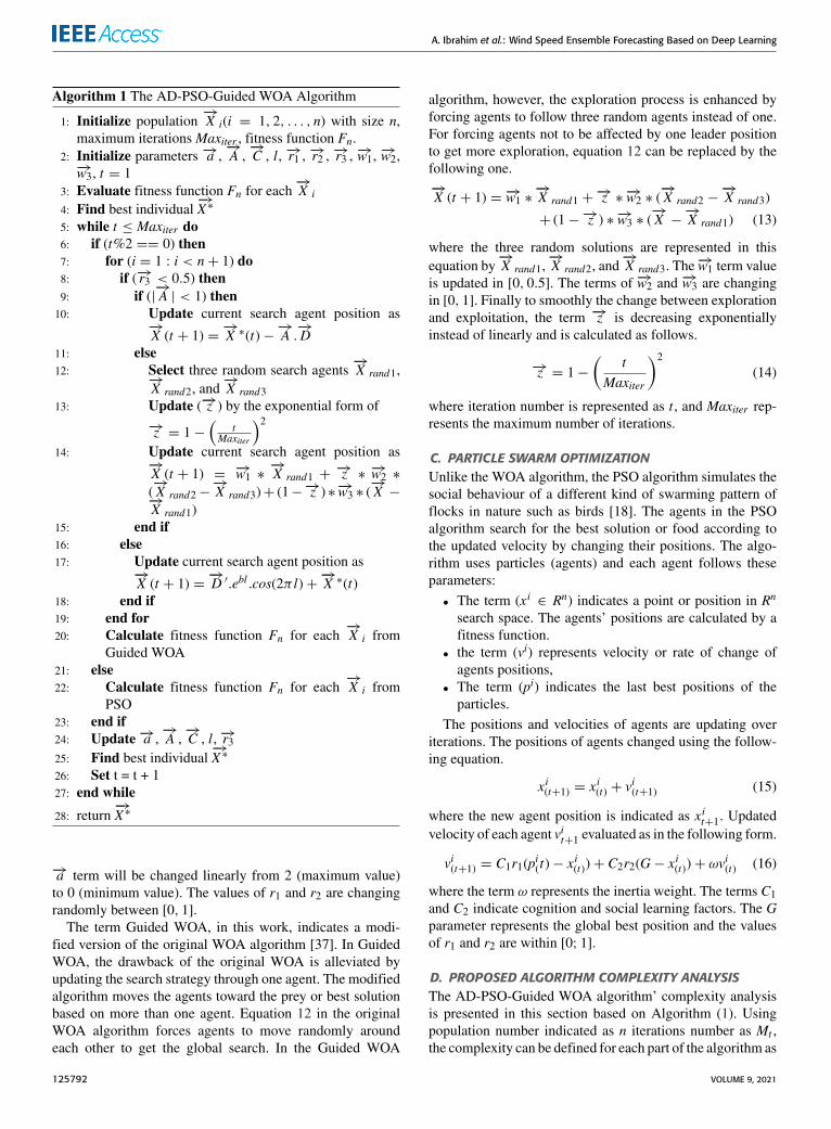
Algorithm 1 The AD-PSO-Guided WOA Algorithm

1: Initialize population−→X i(i = 1, 2, . . . , n) with size n,

maximum iterationsMaxiter , fitness function Fn.2: Initialize parameters −→a ,

−→A ,−→C , l, −→r1 ,

−→r2 ,−→r3 ,−→w1,−→w2,

−→w3, t = 13: Evaluate fitness function Fn for each

−→X i

4: Find best individual−→X∗

5: while t ≤ Maxiter do6: if (t%2 == 0) then7: for (i = 1 : i < n+ 1) do8: if (−→r3 < 0.5) then9: if (|

−→A | < 1) then

10: Update current search agent position as−→X (t + 1) =

−→X ∗(t)−

−→A .−→D

11: else12: Select three random search agents

−→X rand1,

−→X rand2, and

−→X rand3

13: Update (−→z ) by the exponential form of−→z = 1−

(t

Maxiter

)214: Update current search agent position as

−→X (t + 1) = −→w1 ∗

−→X rand1 +

−→z ∗ −→w2 ∗

(−→X rand2−

−→X rand3)+ (1−−→z ) ∗−→w3 ∗ (

−→X −

−→X rand1)

15: end if16: else17: Update current search agent position as

−→X (t + 1) =

−→D ′.ebl .cos(2π l)+

−→X ∗(t)

18: end if19: end for20: Calculate fitness function Fn for each

−→X i from

Guided WOA21: else22: Calculate fitness function Fn for each

−→X i from

PSO23: end if24: Update −→a ,

−→A ,−→C , l, −→r3

25: Find best individual−→X∗

26: Set t = t + 127: end while

28: return−→X∗

−→a term will be changed linearly from 2 (maximum value)to 0 (minimum value). The values of r1 and r2 are changingrandomly between [0, 1].

The term Guided WOA, in this work, indicates a modi-fied version of the original WOA algorithm [37]. In GuidedWOA, the drawback of the original WOA is alleviated byupdating the search strategy through one agent. The modifiedalgorithm moves the agents toward the prey or best solutionbased on more than one agent. Equation 12 in the originalWOA algorithm forces agents to move randomly aroundeach other to get the global search. In the Guided WOA

algorithm, however, the exploration process is enhanced byforcing agents to follow three random agents instead of one.For forcing agents not to be affected by one leader positionto get more exploration, equation 12 can be replaced by thefollowing one.−→X (t + 1) = −→w1 ∗

−→X rand1 +

−→z ∗ −→w2 ∗ (−→X rand2 −

−→X rand3)

+ (1−−→z ) ∗ −→w3 ∗ (−→X −−→X rand1) (13)

where the three random solutions are represented in thisequation by

−→X rand1,

−→X rand2, and

−→X rand3. The

−→w1 term valueis updated in [0, 0.5]. The terms of −→w2 and −→w3 are changingin [0, 1]. Finally to smoothly the change between explorationand exploitation, the term −→z is decreasing exponentiallyinstead of linearly and is calculated as follows.

−→z = 1−(

tMaxiter

)2

(14)

where iteration number is represented as t , and Maxiter rep-resents the maximum number of iterations.

C. PARTICLE SWARM OPTIMIZATIONUnlike the WOA algorithm, the PSO algorithm simulates thesocial behaviour of a different kind of swarming pattern offlocks in nature such as birds [18]. The agents in the PSOalgorithm search for the best solution or food according tothe updated velocity by changing their positions. The algo-rithm uses particles (agents) and each agent follows theseparameters:• The term (x i ∈ Rn) indicates a point or position in Rn

search space. The agents’ positions are calculated by afitness function.

• the term (vi) represents velocity or rate of change ofagents positions,

• The term (pi) indicates the last best positions of theparticles.

The positions and velocities of agents are updating overiterations. The positions of agents changed using the follow-ing equation.

x i(t+1) = x i(t) + vi(t+1) (15)

where the new agent position is indicated as x it+1. Updatedvelocity of each agent vit+1 evaluated as in the following form.

vi(t+1) = C1r1(pi(t)− xi(t))+ C2r2(G− x i(t))+ ωv

i(t) (16)

where the term ω represents the inertia weight. The terms C1and C2 indicate cognition and social learning factors. The Gparameter represents the global best position and the valuesof r1 and r2 are within [0; 1].

D. PROPOSED ALGORITHM COMPLEXITY ANALYSISThe AD-PSO-Guided WOA algorithm’ complexity analysisis presented in this section based on Algorithm (1). Usingpopulation number indicated as n iterations number as Mt ,the complexity can be defined for each part of the algorithm as

125792 VOLUME 9, 2021

A. Ibrahim et al.: Wind Speed Ensemble Forecasting Based on Deep Learning

FIGURE 3. Dynamic updating of the exploration and exploitation groups in the AD-PSO-Guided WOA algorithm.

• Initializing of the population: O (1).• Initializing of parameters −→a ,

−→A ,−→C , l, −→r1 ,

−→r2 ,−→r3 ,−→w1,

−→w2,−→w3, t = 1: O (1).

• Evaluating fitness function Fn: O (n).• Getting best individual

−→X∗: O (n).

• Updating positions: O (Mt × n).• Evaluating agents’ fitness function using Guided WOA:O (Mt × n).

• Evaluating agents’ fitness function using PSO: O (Mt ×

n).• Updating parameters −→a ,

−→A ,−→C , l, −→r3 : O (Mt ).

• Updating best solution: O (Mt × n).• Increasing iteration counter: O (Mt ).

The complexity of the AD-PSO-Guided WOA algorithm canbe considered as O (Mt × n). For m variables problems,the algorithm complexity can be considered O (Mt × n×m).

E. BINARY OPTIMIZERFor the feature selection problem, the output solution shouldbe changed to a binary solution using 0 or 1. The sigmoidfunction is usually employed to change the continuous solu-tion of the optimizer to a binary solution.

−→X (t+1)d =

{0 if Sigmoid(XBest ) < 0.51 otherwise,

Sigmoid(XBest ) =1

1+ e−10(XBest−0.5)(17)

where the best position is indicated asXBest for t iteration. TheSigmoid function is used to help in changing the continuousvalues to be 0 or 1. For Sigmoid(XBest ) ≥ 0.5, the value willchange to 1, otherwise, the value will be changed to be 0.

Algorithm 2 Binary AD-PSO-Guided WOA Algorithm1: Initialize AD-PSO-Guided WOA algorithm configura-

tion, including population and parameters2: Change current solutions to binary solution (0 or 1)3: Evaluate fitness function and determine the best solution

4: Train k-NN based model and then calculate error5: while t ≤ itersmax do6: Apply AD-PSO-Guided WOA algorithm7: Change updated solution to binary solution (0 or

1) based on equation 178: Evaluate fitness function for each agent9: Update parameters

10: Update best solution11: end while12: Return optimal solution

Algorithm (2) shows the step by step explanation of the binaryAD-PRS-Guided WOA Algorithm.

F. FITNESS FUNCTIONThe solutions’ quality of an optimizer is measured basedon the assigned fitness function. The function is mainlydepending on the error rate of classification/regression andthe features that have been selected from the input dataset.The best solution is according to the set of features that cangive a minimum features with a minimum classification errorrate. The following equation is applied in this work for theevaluation of solutions’ quality.

Fn = αErr(O)+ β|s||f |

(18)

VOLUME 9, 2021 125793

A. Ibrahim et al.: Wind Speed Ensemble Forecasting Based on Deep Learning

where the optimizer error rate is indicated as Err(O),the selected set of features is denoted as s, f represents totalnumber of existing features. The α ∈ [0, 1], β = 1 − h1values are responsible of the classification error rate and thenumber of selected features.

IV. EXPERIMENTAL RESULTSThe experimental settings and results for wind power fore-casting problems using the presented AD-PSO-GuidedWOAalgorithm are presented in this section. The dataset is firstdiscussed, and then the experiments are divided into featureselection, ensemble, and comparison scenarios.

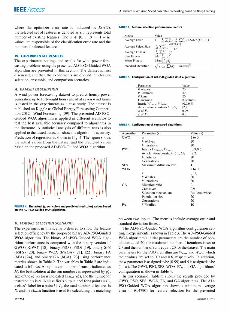
A. DATASET DESCRIPTIONA wind power forecasting dataset to predict hourly powergeneration up to forty-eight hours ahead at seven wind farmsis tested in the experiments as a case study. The dataset ispublished on Kaggle as Global Energy Forecasting Competi-tion 2012 - Wind Forecasting [39]. The presented AD-PSO-Guided WOA algorithm is applied in different scenarios totest the best available accuracy compared to algorithms inthe literature. A statistical analysis of different tests is alsoapplied to the tested dataset to show the algorithm’s accuracy.Prediction of regression is shown in Fig. 4. The figure showsthe actual values from the dataset and the predicted valuesbased on the proposed AD-PSO-Guided WOA algorithm.

FIGURE 4. The actual (green color) and predicted (red color) values basedon the AD-PSO-Guided WOA algorithm.

B. FEATURE SELECTION SCENARIOThe experiment in this scenario desired to show the featureselection efficiency by the proposed binary AD-PSO-GuidedWOA algorithm. The binary AD-PSO-Guided WOA algo-rithm performance is compared with the binary version ofGWO (bGWO) [18], binary PSO (bPSO) [19], binary SFS(bSFS) [20], binary WOA (bWOA) [21], [22], binary FA(bFA) [24], and binary GA (bGA) [23] using performancemetrics shown in Table 2. The variables in Table 2 are indi-cated as follows. An optimizer number of runs is indicated asM , the best solution at the run number j is represented by g∗j ,size of the g∗j vector is indicated as size(g

∗j ), and the number of

tested points isN . A classifier’s output label for a point i isCi,a class’s label for a point i is Li, the total number of features isD, and theMatch function is used for calculating thematching

TABLE 2. Feature selection performance metrics.

TABLE 3. Configuration of AD-PSO-guided WOA algorithm.

TABLE 4. Configuration of compared algorithms.

between two inputs. The metrics include average error andstandard deviation fitness.

The AD-PSO-Guided WOA algorithm configuration set-ting in experiments is shown in Table 3. TheAD-PSO-GuidedWOA algorithm’s initial parameters are the number of pop-ulation equal 20, the maximum number of iterations is set to20, and the number of runs equals 20 for the dataset. Themainparameters for the PSO algorithm areWmax andWmin, whichtheir values are set to 0.9 and 0.6, respectively. In addition,theα parameter is assigned to be (0.99) andβ is assigned to be(1−α). The GWO, PSO, SFS,WOA, FA, andGA algorithms’configuration is shown in Table 4.

In this scenario, Table 5 shows the results provided byGWO, PSO, SFS, WOA, FA, and GA algorithms. The AD-PSO-Guided WOA algorithm shows a minimum averageerror of (0.4790) for feature selection for the presented

125794 VOLUME 9, 2021

A. Ibrahim et al.: Wind Speed Ensemble Forecasting Based on Deep Learning

TABLE 5. Results of feature selection for the presented and compared binary algorithms.

TABLE 6. Results of ANOVA test for feature selection of the presented and compared binary algorithms.

TABLE 7. One sample t-test for feature selection of the presented and compared binary algorithms.

FIGURE 5. The AD-PSO-Guided WOA algorithm convergence curvecompared to different algorithms.

results. The AD-PSO-Guided WOA algorithm, based on theminimum error of the tested problem, is the best and the SFSalgorithm is the worst. In terms of standard deviation, the AD-PSO-GuidedWOAalgorithm has the lowest value of (0.1635)which indicates the algorithm’s stability and robustness.

The convergence curve of the AD-PSO-Guided WOAalgorithm compared to other algorithms is shown in Figure 5.The figure shows the exploitation capability of the algorithmand its ability to avoid possible local optima that can beoccurred during the optimization process. Figure 6 shows theAD-PSO-Guided WOA average error based on the objectivefunction compared to different algorithms. The minimum,maximum, and average values for different binary algorithms

FIGURE 6. The AD-PSO-Guided WOA algorithm average error based onthe objective function compared to different binary algorithms.

indicate the advantages of the presented algorithm. Thep-values of the AD-PSO-Guided WOA algorithm are testedcompared to GWO, PSO, SFS,WOA, FA, and GA algorithmsbyANOVA and t-test tests in Tables 6 and 7, respectively. The

VOLUME 9, 2021 125795

A. Ibrahim et al.: Wind Speed Ensemble Forecasting Based on Deep Learning

FIGURE 7. Residual, heteroscedasticity, QQ plots and heat map of the presented and compared algorithms forfeature selection problem.

statistical analysis results show the superiority and statisticalsignificance of the suggested algorithm.

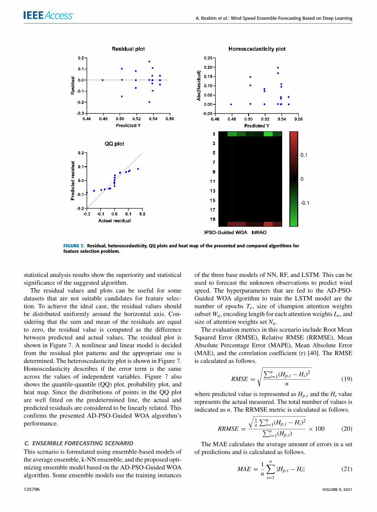
The residual values and plots can be useful for somedatasets that are not suitable candidates for feature selec-tion. To achieve the ideal case, the residual values shouldbe distributed uniformly around the horizontal axis. Con-sidering that the sum and mean of the residuals are equalto zero, the residual value is computed as the differencebetween predicted and actual values. The residual plot isshown in Figure 7. A nonlinear and linear model is decidedfrom the residual plot patterns and the appropriate one isdetermined. The heteroscedasticity plot is shown in Figure 7.Homoscedasticity describes if the error term is the sameacross the values of independent variables. Figure 7 alsoshows the quantile-quantile (QQ) plot, probability plot, andheat map. Since the distributions of points in the QQ plotare well fitted on the predetermined line, the actual andpredicted residuals are considered to be linearly related. Thisconfirms the presented AD-PSO-Guided WOA algorithm’sperformance.

C. ENSEMBLE FORECASTING SCENARIOThis scenario is formulated using ensemble-based models ofthe average ensemble, k-NN ensemble, and the proposed opti-mizing ensemble model based on the AD-PSO-GuidedWOAalgorithm. Some ensemble models use the training instances

of the three base models of NN, RF, and LSTM. This can beused to forecast the unknown observations to predict windspeed. The hyperparameters that are fed to the AD-PSO-Guided WOA algorithm to train the LSTM model are thenumber of epochs Te, size of champion attention weightssubsetWa, encoding length for each attention weights Le, andsize of attention weights set Na.The evaluation metrics in this scenario include Root Mean

Squared Error (RMSE), Relative RMSE (RRMSE), MeanAbsolute Percentage Error (MAPE), Mean Absolute Error(MAE), and the correlation coefficient (r) [40]. The RMSEis calculated as follows.

RMSE =

√∑ni=1(Hp,i − Hi)

2

n(19)

where predicted value is represented as Hp,i and the Hi valuerepresents the actual measured. The total number of values isindicated as n. The RRMSE metric is calculated as follows.

RRMSE =

√1n

∑ni=1(Hp,i − Hi)2∑ni=1(Hp,i)

× 100 (20)

The MAE calculates the average amount of errors in a setof predictions and is calculated as follows.

MAE =1n

n∑i=1

|Hp,i − Hi| (21)

125796 VOLUME 9, 2021

A. Ibrahim et al.: Wind Speed Ensemble Forecasting Based on Deep Learning

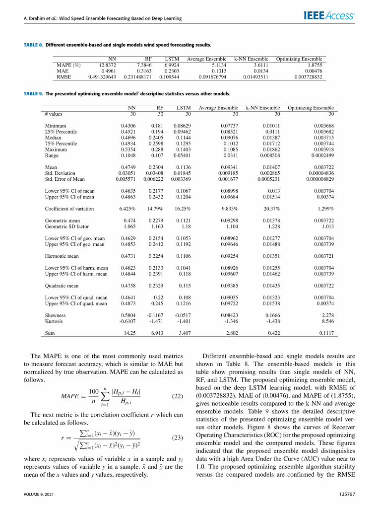
TABLE 8. Different ensemble-based and single models wind speed forecasting results.

TABLE 9. The presented optimizing ensemble model’ descriptive statistics versus other models.

The MAPE is one of the most commonly used metricsto measure forecast accuracy, which is similar to MAE butnormalized by true observation. MAPE can be calculated asfollows.

MAPE =100n

n∑i=1

|Hp,i − Hi|Hp,i

(22)

The next metric is the correlation coefficient r which canbe calculated as follows.

r =

∑ni=1(xi − x)(yi − y)√∑ni=1(xi − x)2(yi − y)2

(23)

where xi represents values of variable x in a sample and yirepresents values of variable y in a sample. x and y are themean of the x values and y values, respectively.

Different ensemble-based and single models results areshown in Table 8. The ensemble-based models in thistable show promising results than single models of NN,RF, and LSTM. The proposed optimizing ensemble model,based on the deep LSTM learning model, with RMSE of(0.003728832), MAE of (0.00476), and MAPE of (1.8755),gives noticeable results compared to the k-NN and averageensemble models. Table 9 shows the detailed descriptivestatistics of the presented optimizing ensemble model ver-sus other models. Figure 8 shows the curves of ReceiverOperating Characteristics (ROC) for the proposed optimizingensemble model and the compared models. These figuresindicated that the proposed ensemble model distinguishesdata with a high Area Under the Curve (AUC) value near to1.0. The proposed optimizing ensemble algorithm stabilityversus the compared models are confirmed by the RMSE

VOLUME 9, 2021 125797

A. Ibrahim et al.: Wind Speed Ensemble Forecasting Based on Deep Learning

FIGURE 8. The presented optimizing ensemble model’s ROC curves versus other models.

TABLE 10. ANOVA results of the base and ensemble models for the wind speed forecasting.

TABLE 11. Wilcoxon signed rank test results of the base and ensemble models for the wind speed forecasting.

distribution, shown in Figure 9, the histogram of RMSE,shown in Figure 10, the histogram of RRMSE, shown inFigure 11, and the histogram of MAPE, shown in Figure 12.

Tests of ANOVA and Wilcoxon’s rank-sum are applied inthis scenario to evaluate the statistical differences between the

presented and compared models. ANOVA output results areshown in Table 10. Wilcoxon’s rank-sum statistical analysispresented in Table 11 determines if the models’ results havea significant difference. For p-value < 0.05, this indicatessignificant superiority. The results show the AD-PSO-Guided

125798 VOLUME 9, 2021

A. Ibrahim et al.: Wind Speed Ensemble Forecasting Based on Deep Learning

FIGURE 9. RMSE based on objective function of the presented optimizingensemble model and other models.

FIGURE 10. Histogram of RMSE of the presented optimizing ensemblemodel and other models with Bin Center range of (0.00 - 0.59) based onnumber of values.

WOA algorithm-based proposed ensemble model superiorityand also show the algorithm’s statistical significance.

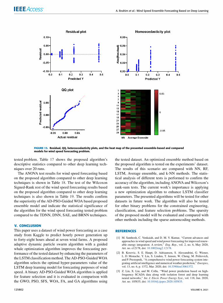
The residual plot in this scenario is shown in Figure 13.The heteroscedasticity plot, QQ plot, and heat map are alsoshown in Figure 13. Since the distributions of points in theQQplot are well fitted on the line, the predicted and the actualresiduals are considered as linearly related which confirmsthe proposed AD-PSO-Guided WOA ensemble-based algo-rithm’s performance for the wind speed forecasting problem.

D. COMPARISONS SCENARIOThe third and last scenario is designed to show the perfor-mance of the optimizing ensemble-based AD-PSO-GuidedWOA algorithm compared with PSO [19], WOA [22],GA [23], GWO [18], HHO [25], [26], MPA [28], ChOA [29],

FIGURE 11. Histogram of RRMSE of the presented optimizing ensemblemodel and other models with Bin Center range of (1.0 - 51.5) based onnumber of values.

FIGURE 12. Histogram of MAPE of the presented optimizing ensemblemodel and other models with Bin Center range of (1.8 - 14.8) based onnumber of values.

and SMA [27]. The AD-PSO-Guided WOA algorithmensemble model is also compared with four deep learningtechniques including TDNN [30], DNN [31], SAE [32], andBRNN [33].

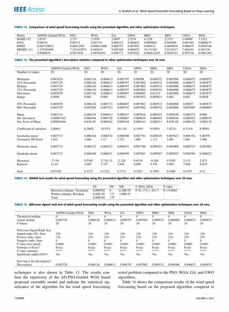
Table 12 shows the comparison results of the wind speedforecasting based on the proposed algorithm compared toother optimization techniques. The results in the table showthat the presented optimizing ensemble model, based on theLSTM deep learning model and the AD-PSO-Guided WOAalgorithm, gives competitive results with MAPE of (1.8755),MAE of (0.00476), RMSE of (0.003728832), RRMSE of(1.279369489), and r of (0.9998878) compared to otheralgorithms for the wind speed forecasting tested problem.Table 13 shows the proposed algorithm’s descriptive statisticscompared to other optimization techniques over 20 runs.

The ANOVA test results for wind speed forecasting basedon the proposed algorithm compared to other optimizationtechniques is shown in Table 14. The test of the WilcoxonSigned-Rank rest of the wind speed forecasting results basedon the proposed algorithm compared to other optimization

VOLUME 9, 2021 125799

A. Ibrahim et al.: Wind Speed Ensemble Forecasting Based on Deep Learning

TABLE 12. Comparison of wind speed forecasting results using the presented algorithm and other optimization techniques.

TABLE 13. The presented algorithm’s description statistics compared to other optimization techniques over 20 runs.

TABLE 14. ANOVA test results for wind speed forecasting using the presented algorithm and other optimization techniques over 20 runs.

TABLE 15. Wilcoxon signed rank test of wind speed forecasting results using the presented algorithm and other optimization techniques over 20 runs.

techniques is also shown in Table 15. The results con-firm the superiority of the AD-PSO-Guided WOA basedproposed ensemble model and indicate the statistical sig-nificance of the algorithm for the wind speed forecasting

tested problem compared to the PSO, WOA, GA, and GWOalgorithms.

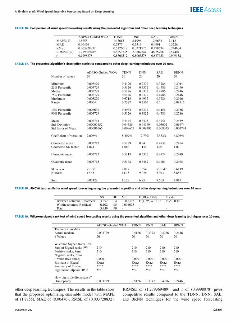
Table 16 shows the comparison results of the wind speedforecasting based on the proposed algorithm compared to

125800 VOLUME 9, 2021

A. Ibrahim et al.: Wind Speed Ensemble Forecasting Based on Deep Learning

TABLE 16. Comparison of wind speed forecasting results using the presented algorithm and other deep learning techniques.

TABLE 17. The presented algorithm’s description statistics compared to other deep learning techniques over 20 runs.

TABLE 18. ANOVA test results for wind speed forecasting using the presented algorithm and other deep learning techniques over 20 runs.

TABLE 19. Wilcoxon signed rank test of wind speed forecasting results using the presented algorithm and other deep learning techniques over 20 runs.

other deep learning techniques. The results in the table showthat the proposed optimizing ensemble model with MAPEof (1.8755), MAE of (0.00476), RMSE of (0.003728832),

RRMSE of (1.279369489), and r of (0.9998878) givescompetitive results compared to the TDNN, DNN, SAE,and BRNN techniques for the wind speed forecasting

VOLUME 9, 2021 125801

A. Ibrahim et al.: Wind Speed Ensemble Forecasting Based on Deep Learning

FIGURE 13. Residual, QQ, heteroscedasticity plots, and the heat map of the presented ensemble-based and comparedmodels for wind speed forecasting problem.

tested problem. Table 17 shows the proposed algorithm’sdescriptive statistics compared to other deep learning tech-niques over 20 runs.

The ANOVA test results for wind speed forecasting basedon the proposed algorithm compared to other deep learningtechniques is shown in Table 18. The test of the WilcoxonSigned-Rank rest of the wind speed forecasting results basedon the proposed algorithm compared to other deep learningtechniques is also shown in Table 19. The results confirmthe superiority of the AD-PSO-GuidedWOA based proposedensemble model and indicate the statistical significance ofthe algorithm for the wind speed forecasting tested problemcompared to the TDNN, DNN, SAE, and BRNN techniques.

V. CONCLUSIONThis paper uses a dataset of wind power forecasting as a casestudy from Kaggle to predict hourly power generation upto forty-eight hours ahead at seven wind farms. A proposedadaptive dynamic particle swarm algorithm with a guidedwhale optimization algorithm improves the forecasting per-formance of the tested dataset by enhancing the parameters ofthe LSTMclassificationmethod. TheAD-PSO-GuidedWOAalgorithm selects the optimal hyper-parameters value of theLSTM deep learning model for forecasting purposes of windspeed. A binary AD-PSO-Guided WOA algorithm is appliedfor feature selection and it is evaluated in comparison withthe GWO, PSO, SFS, WOA, FA, and GA algorithms using

the tested dataset. An optimized ensemble method based onthe proposed algorithm is tested on the experiments’ dataset.The results of this scenario are compared with NN, RF,LSTM, Average ensemble, and k-NN methods. The statis-tical analysis of different tests is performed to confirm theaccuracy of the algorithm, including ANOVA andWilcoxon’srank-sum tests. The current work’s importance is applyinga new optimization algorithm to enhance LSTM classifierparameters. The presented algorithms will be tested for otherdatasets in future work. The algorithm will also be testedfor other binary problems for the constrained engineering,classification, and feature selection problems. The sparsityof the proposed model will be evaluated and compared withother methods including the sparse autoencoding methods.

REFERENCES

[1] M. Santhosh, C. Venkaiah, and D. M. V. Kumar, ‘‘Current advances andapproaches in wind speed and wind power forecasting for improved renew-able energy integration: A review,’’ Eng. Rep., vol. 2, no. 6, May 2020,Art. no. e12178, doi: 10.1002/eng2.12178.

[2] B. Kosovic, S. E. Haupt, D. Adriaansen, S. Alessandrini, G. Wiener,L. D. Monache, Y. Liu, S. Linden, T. Jensen, W. Cheng, M. Politovich,and P. Prestopnik, ‘‘A comprehensive wind power forecasting system inte-grating artificial intelligence and numerical weather prediction,’’ Energies,vol. 13, no. 6, p. 1372, Mar. 2020, doi: 10.3390/en13061372.

[3] Z. Lin, X. Liu, and M. Collu, ‘‘Wind power prediction based on high-frequency SCADA data along with isolation forest and deep learningneural networks,’’ Int. J. Electr. Power Energy Syst., vol. 118, Jun. 2020,Art. no. 105835, doi: 10.1016/j.ijepes.2020.105835.

125802 VOLUME 9, 2021

A. Ibrahim et al.: Wind Speed Ensemble Forecasting Based on Deep Learning

[4] M. Ibrahim, A. Alsheikh, Q. Al-Hindawi, S. Al-Dahidi, and H. ElMoaqet,‘‘Short-time wind speed forecast using artificial learning-based algo-rithms,’’ Comput. Intell. Neurosci., vol. 2020, pp. 1–15, Apr. 2020, doi:10.1155/2020/8439719.

[5] J. M. Lima, A. K. Guetter, S. R. Freitas, J. Panetta, and J. G. Z. de Mattos,‘‘Ameteorological–statisticmodel for short-termwind power forecasting,’’J. Control, Autom. Electr. Syst., vol. 28, no. 5, pp. 679–691, Jul. 2017, doi:10.1007/s40313-017-0329-8.

[6] J. Liu, X. Wang, and Y. Lu, ‘‘A novel hybrid methodology for short-term wind power forecasting based on adaptive neuro-fuzzy infer-ence system,’’ Renew. Energy, vol. 103, pp. 620–629, Apr. 2017, doi:10.1016/j.renene.2016.10.074.

[7] M. Khodayar, J.Wang, andM.Manthouri, ‘‘Interval deep generative neuralnetwork for wind speed forecasting,’’ IEEE Trans. Smart Grid, vol. 10,no. 4, pp. 3974–3989, Jul. 2019, doi: 10.1109/TSG.2018.2847223.

[8] M. Khodayar, O. Kaynak, and M. E. Khodayar, ‘‘Rough deep neural archi-tecture for short-termwind speed forecasting,’’ IEEE Trans. Ind. Informat.,vol. 13, no. 6, pp. 2770–2779, Dec. 2017, doi: 10.1109/TII.2017.2730846.

[9] M. Khodayar and J. Wang, ‘‘Spatio-temporal graph deep neural networkfor short-term wind speed forecasting,’’ IEEE Trans. Sustain. Energy,vol. 10, no. 2, pp. 670–681, Apr. 2019, doi: 10.1109/TSTE.2018.2844102.

[10] S. M. J. Jalali, S. Ahmadian, M. Khodayar, A. Khosravi, V. Ghasemi,M. Shafie-Khah, S. Nahavandi, and J. P. S. Catalão, ‘‘Towards noveldeep neuroevolution models: Chaotic levy grasshopper optimization forshort-term wind speed forecasting,’’ Eng. Comput., vol. 2021, pp. 1–25,Mar. 2021, doi: 10.1007/s00366-021-01356-0.

[11] H. S. Dhiman, D. Deb, and J. M. Guerrero, ‘‘Hybrid machine intel-ligent SVR variants for wind forecasting and ramp events,’’ Renew.Sustain. Energy Rev., vol. 108, pp. 369–379, Jul. 2019, doi: 10.1016/j.rser.2019.04.002.

[12] H. S. Dhiman and D. Deb, ‘‘Machine intelligent and deep learning tech-niques for large training data in short-term wind speed and ramp eventforecasting,’’ Int. Trans. Electr. Energy Syst., Feb. 2021, Art. no. e12818,doi: 10.1002/2050-7038.12818.

[13] H. S. Dhiman, D. Deb, S. M. Muyeen, and I. Kamwa, ‘‘Wind turbine gear-box anomaly detection based on adaptive threshold and twin support vectormachines,’’ IEEE Trans. Energy Convers., early access, Apr. 27, 2021, doi:10.1109/TEC.2021.3075897.

[14] B. Bilal, M. Ndongo, K. H. Adjallah, A. Sava, C. M. F. Kebe, P. A. Ndiaye,and V. Sambou, ‘‘Wind turbine power output prediction model designbased on artificial neural networks and climatic spatiotemporal data,’’ inProc. IEEE Int. Conf. Ind. Technol. (ICIT), Feb. 2018, pp. 1085–1092, doi:10.1109/ICIT.2018.8352329.

[15] J. Wang, W. Yang, P. Du, and Y. Li, ‘‘Research and application of ahybrid forecasting framework based on multi-objective optimization forelectrical power system,’’ Energy, vol. 148, pp. 59–78, Apr. 2018, doi:10.1016/j.energy.2018.01.112.

[16] Y.-Y. Hong, C. L. Paulo, and P. Rioflorido, ‘‘A hybrid deep learning-based neural network for 24-h ahead wind power forecasting,’’ Appl.Energy, vol. 250, no. 15, pp. 530–539, Sep. 2019, doi: 10.1016/j.apenergy.2019.05.044.

[17] J. Zhang, J. Yan, D. Infield, Y. Liu, and F.-S. Lien, ‘‘Short-term forecastingand uncertainty analysis of wind turbine power based on long short-termmemory network and Gaussian mixture model,’’ Appl. Energy, vol. 241,pp. 229–244, May 2019, doi: 10.1016/j.apenergy.2019.03.044.

[18] E.-S. M. El-Kenawy and M. Eid, ‘‘Hybrid gray wolf and particle swarmoptimization for feature selection,’’ Int. J. Innov. Comput. Inf. Control,vol. 16, no. 3, pp. 831–844, 2020.

[19] R. Bello, Y. Gomez, A.Nowe, andM.M.Garcia, ‘‘Two-step particle swarmoptimization to solve the feature selection problem,’’ in Proc. 7th Int. Conf.Intell. Syst. Design Appl. (ISDA), Oct. 2007, pp. 691–696.

[20] E.-S.M. El-Kenawy, A. Ibrahim, S.Mirjalili, M.M. Eid, and S. E. Hussein,‘‘Novel feature selection and voting classifier algorithms for COVID-19classification in CT images,’’ IEEE Access, vol. 8, pp. 179317–179335,2020, doi: 10.1109/ACCESS.2020.3028012.

[21] S. Mirjalili and A. Lewis, ‘‘The whale optimization algorithm,’’Adv. Eng. Softw., vol. 95, pp. 51–67, May 2016. [Online]. Available:http://www.sciencedirect.com/science/article/pii/S0965997816300163

[22] E. M. Hassib, A. I. El-Desouky, L. M. Labib, and E.-S.-M. El-Kenawy,‘‘WOA + BRNN: An imbalanced big data classification framework usingwhale optimization and deep neural network,’’ Soft Comput., vol. 24, no. 8,pp. 5573–5592, Mar. 2019, doi: 10.1007/s00500-019-03901-y.

[23] M. M. Kabir, M. Shahjahan, and K. Murase, ‘‘A new local searchbased hybrid genetic algorithm for feature selection,’’ Neurocomputing,vol. 74, no. 17, pp. 2914–2928, 2011. [Online]. Available: http://www.sciencedirect.com/science/article/pii/S0925231211002748

[24] I. Fister, Jr., X.-S. Yang, I. Fister, and J. Brest, ‘‘Memetic firefly algorithmfor combinatorial optimization,’’ 2012, arXiv:1204.5165. [Online]. Avail-able: http://arxiv.org/abs/1204.5165

[25] A. A. Heidari, S. Mirjalili, H. Faris, I. Aljarah, M. Mafarja, and H. Chen,‘‘Harris hawks optimization: Algorithm and applications,’’ Future Gener.Comput. Syst., vol. 97, pp. 849–872, Aug. 2019, doi: 10.1016/j.future.2019.02.028.

[26] A. Ibrahim, H. A. Ali, M. M. Eid, and E.-S.-M. El-Kenawy, ‘‘ChaoticHarris hawks optimization for unconstrained function optimization,’’ inProc. 16th Int. Comput. Eng. Conf. (ICENCO), Dec. 2020, pp. 153–158,doi: 10.1109/ICENCO49778.2020.9357403.

[27] S. Li, H. Chen, M. Wang, A. A. Heidari, and S. Mirjalili, ‘‘Slimemould algorithm: A new method for stochastic optimization,’’ FutureGener. Comput. Syst., vol. 111, pp. 300–323, Oct. 2020, doi: 10.1016/j.future.2020.03.055.

[28] A. Faramarzi, M. Heidarinejad, S. Mirjalili, and A. H. Gandomi, ‘‘Marinepredators algorithm: A nature-inspired metaheuristic,’’ Expert Syst.Appl., vol. 152, Aug. 2020, Art. no. 113377, doi: 10.1016/j.eswa.2020.113377.

[29] M. Khishe and M. R. Mosavi, ‘‘Chimp optimization algorithm,’’ ExpertSyst. Appl., vol. 149, Jul. 2020, Art. no. 113338, doi: 10.1016/j.eswa.2020.113338.

[30] F. Noman, G. Alkawsi, A. A. Alkahtani, A. Q. Al-Shetwi, S. K. Tiong,N. Alalwan, J. Ekanayake, and A. I. Alzahrani, ‘‘Multistep short-termwind speed prediction using nonlinear auto-regressive neural networkwith exogenous variable selection,’’ Alexandria Eng. J., vol. 60, no. 1,pp. 1221–1229, Feb. 2021, doi: 10.1016/j.aej.2020.10.045.

[31] X. Liu, H. Zhang, X. Kong, and K. Y. Lee, ‘‘Wind speed forecast-ing using deep neural network with feature selection,’’ Neurocom-puting, vol. 397, pp. 393–403, Jul. 2020, doi: 10.1016/j.neucom.2019.08.108.

[32] T. Su, Y. Liu, J. Zhao, and J. Liu, ‘‘Probabilistic stacked denoising autoen-coder for power system transient stability prediction with wind farms,’’IEEE Trans. Power Syst., vol. 36, no. 4, pp. 3786–3789, Jul. 2021, doi:10.1109/TPWRS.2020.3043620.

[33] J. F. Torres, D. Hadjout, A. Sebaa, F. Martínez-Álvarez, and A. Troncoso,‘‘Deep learning for time series forecasting: A survey,’’ Big Data, vol. 9,no. 1, pp. 3–21, Feb. 2021, doi: 10.1089/big.2020.0159.

[34] M. S. Nazir, F. Alturise, S. Alshmrany, H. M. J. Nazir, M. Bilal,A. N. Abdalla, P. Sanjeevikumar, and Z. M. Ali, ‘‘Wind generation fore-casting methods and proliferation of artificial neural network: A review offive years research trend,’’ Sustainability, vol. 12, no. 9, p. 3778,May 2020,doi: 10.3390/su12093778.

[35] E.-S. M. El-Kenawy, S. Mirjalili, A. Ibrahim, M. Alrahmawy, M. El-Said,R. M. Zaki, and M. M. Eid, ‘‘Advanced meta-heuristics, convolutionalneural networks, and feature selectors for efficient COVID-19 X-ray chestimage classification,’’ IEEE Access, vol. 9, pp. 36019–36037, 2021, doi:10.1109/ACCESS.2021.3061058.

[36] A. A. Nasser, M. Z. Rashad, and S. E. Hussein, ‘‘A two-layer waterdemand prediction system in urban areas based on micro-services andLSTM neural networks,’’ IEEE Access, vol. 8, pp. 147647–147661, 2020,doi: 10.1109/ACCESS.2020.3015655.

[37] S. S. M. Ghoneim, T. A. Farrag, A. A. Rashed, E.-S. M. El-Kenawy,and A. Ibrahim, ‘‘Adaptive dynamic meta-heuristics for feature selec-tion and classification in diagnostic accuracy of transformer faults,’’IEEE Access, vol. 9, pp. 78324–78340, 2021, doi: 10.1109/ACCESS.2021.3083593.

[38] S. Mirjalili, S. M. Mirjalili, S. Saremi, and S. Mirjalili, ‘‘Whale opti-mization algorithm: Theory, literature review, and application in designingphotonic crystal filters,’’ Nature-Inspired Optimizers. Cham, Switzerland:Springer, 2020, pp. 219–238, doi: 10.1007/978-3-030-12127-3_13.

[39] Global Energy Forecasting Competition 2012—Wind Forecasting.Accessed: Jun. 19, 2021. [Online]. Available: https://www.kaggle.com/c/GEF2012-wind-forecasting

[40] R. Al-Hajj, A. Assi, and M. M. Fouad, ‘‘Stacking-based ensemble ofsupport vector regressors for one-day ahead solar irradiance prediction,’’in Proc. 8th Int. Conf. Renew. Energy Res. Appl. (ICRERA), Nov. 2019,pp. 428–433, doi: 10.1109/ICRERA47325.2019.8996629.

VOLUME 9, 2021 125803

A. Ibrahim et al.: Wind Speed Ensemble Forecasting Based on Deep Learning

ABDELHAMEED IBRAHIM (Member, IEEE)received the bachelor’s and master’s degrees inengineering from the Computer Engineering andSystems Department, in 2001 and 2005, respec-tively, and the Ph.D. degree in engineering fromthe Faculty of Engineering, Chiba University,Japan, in 2011. He was with the Faculty ofEngineering, Mansoura University, Egypt, from2001 to 2007, where he is currently an Asso-ciate Professor of computer engineering. He has

published over 50 publications with over 1000 citations and an H-indexof 19. His research interests include machine learning, optimization, swarmintelligence, and pattern recognition. He serves as a Reviewer for Journalof Electronic Imaging, IEEE ACCESS, Computer Standards and Interfaces,Optical Engineering, IEEE JOURNAL OF BIOMEDICAL AND HEALTH INFORMATICS,Biomedical Signal Processing and Control, IET Image Processing, Multi-media Tools and Applications, Frontiers of Information Technology & Elec-tronic Engineering, Journal of Healthcare Engineering, and other respectedjournals.

SEYEDALI MIRJALILI (Senior Member, IEEE) iscurrently the Director of the Centre for ArtificialIntelligence Research and Optimization, TorrensUniversity Australia, Brisbane. He has publishedover 200 publications with over 36,000 citationsand an H-index of 65. As the most cited researcherin robust optimization, he is in the list of 1% highlycited researchers and named as one of the mostinfluential researchers in the world by the Web ofScience. He is also internationally recognized for

his advances in swarm intelligence and optimization, including the first setof algorithms from a synthetic intelligence standpoint—a radical departurefrom how natural systems are typically understood—and a systematic designframework to reliably benchmark, evaluate, and propose computationallycheap robust optimization algorithms. He is also working on the applicationsof multi-objective and robust meta-heuristic optimization techniques as well.His research interests include robust optimization, engineering optimization,multi-objective optimization, swarm intelligence, evolutionary algorithms,and artificial neural networks. He is also an Associate Editor of severaljournals, including Applied Soft Computing, Neurocomputing, Applied Intel-ligence, Advances in Engineering Software, IEEE ACCESS, and PLOS One.

M. EL-SAID received the B.Sc. (Hons.), M.Sc.,and Ph.D. degrees in electric power engineer-ing from Mansoura University, Egypt, in 1981,1987, and 1992, respectively. He is currently theDean of the Delta Higher Institute of Engineer-ing and Technology, Ministry of Higher Educa-tion, Egypt. He is also an Official Reviewer forEgyptian Universities Promotion Committees—Supreme Council of Universities in Egypt. He hasbeen a Professor of electric power systemswith the

Department of Electrical Engineering, Faculty of Engineering, MansouraUniversity, since 2005. He was the Vice-Dean of the Community Servicesand Environmental Development, Faculty of Engineering, Mansoura Uni-versity, from 2010 to 2011. He was also the Director of the Communicationand Information Technology Centre (CITC), Mansoura University, from2014 to 2016. From 2016 to 2018, he was the Dean of the Faculty ofEngineering, Mansoura University. His research interests include renewableenergy, smart grids, and power system operation and control. He is also aReviewer of scientific journals, including Electric Power Components andSystems, IEEE TRANSACTIONS ON POWER SYSTEMS, and IEEE TRANSACTIONS ON

POWER DELIVERY.

SHERIF S. M. GHONEIM (Senior Member,IEEE) received the B.Sc. and M.Sc. degrees fromthe Faculty of Engineering at Shoubra, ZagazigUniversity, Egypt, in 1994 and 2000, respectively,and the Ph.D. degree in electrical power andmachines from the Faculty of Engineering, CairoUniversity, in 2008. Since 1996, he has beenteaching with the Faculty of Industrial Educa-tion, Suez Canal University, Egypt. From 2005 to2007, he was a Guest Researcher with the Institute

of Energy Transport and Storage (ETS), University of Duisburg–Essen,Germany. He joined the Electrical Engineering Department, Faculty of Engi-neering, Taif University, as an Associate Professor. His research interestsinclude grounding systems, breakdown in SF6 gas, dissolved gas analysis,and AI technique applications.

MOSLEH M. AL-HARTHI was born in Taif, SaudiArabia, in October 1966. He received the B.Sc.and M.S. degrees in electronics technology andengineering from Indiana State University, TerreHaute, USA, in 1996 and 1997, respectively, andthe Ph.D. degree in electrical engineering fromArkansas University, Fayetteville, USA, in 2001.He was an Assistant Professor with the College ofTechnology, Jeddah, Saudi Arabia, from 2001 to2009. He is currently working as an Associate

Professor with the Electrical Engineering Department, Taif University, SaudiArabia. His research interests include electronics, control engineering, andsignal processing.

TAREK F. IBRAHIM received the Ph.D. degreein pure mathematics from the Faculty of Science,Mansoura University, Egypt, in 2006. He is cur-rently an Associate Professor of pure mathematics.He has published over 47 publications with over538 citations and an H-index of 14. His researchinterests include difference equations and theirtopics in engineering and physics. He serves asa Reviewer for many international journals, suchas Mathematical Problems in Engineering, Math-

ematical Methods in the Applied Sciences, British Journal of Mathematics& Computer Science, and other respected journals.

EL-SAYED M. EL-KENAWY (Member, IEEE) iscurrently an Assistant Professor with the DeltaHigher Institute for Engineering and Technology(DHIET), Mansoura, Egypt. He published morethan 35 articles with more than 750 citations andan H-index of 19. He has launched and pioneeredindependent research programs. He is also moti-vating and inspiring his students by different waysby providing a thorough understanding of a vari-ety of computer concepts and explains complex

concepts in an easy-to-understand manner. His research interests includeartificial intelligence, machine learning, optimization, deep learning, digitalmarketing, and data science. He is also a Reviewer for Computers, Materials& Continua journal, IEEE ACCESS, and some other journals.

125804 VOLUME 9, 2021