???? 1

Abstract— Power curves constructed from wind speed and

active power output measurements provide an establishedmethod of analyzing wind turbine performance. In this paper it isproposed that operational data from wind turbines are used toestimate bivariate probability distribution functions representingthe power curve of existing turbines so that deviations fromexpected behavior can be detected. Owing to the complex form ofdependency between active power and wind speed, which noclassical parameterized distribution can approximate, theapplication of empirical copulas is proposed; the statistical theoryof copulas allows the distribution form of marginal distributionsof wind speed and power to be expressed separately frominformation about the dependency between them. Copulaanalysis is discussed in terms of its likely usefulness in windturbine condition monitoring, particularly in early recognition ofincipient faults such as blade degradation, yaw and pitch errors.

Index Terms— Wind power generation, Energy conversion,Power generation reliability.

I. INTRODUCTION

IND power based renewable energy has seen dramaticgrowth over the past decade, which is set to continue asmany countries implement stringent targets for

sustainability and emissions reduction. The UK government isaiming to generate 20% of the country’s electricity from windturbines by 2020, up from 3% in 2008 [1] to form part of theEuropean Union’s target of producing 20% of all energy fromrenewable sources [2]. A supporting trend in wind generationis the move towards larger turbines in offshore locations.Notable examples include Danish plans to double offshorewind capacity from 661MW to 1256MW over the coming fouryears [3] and plans for 25 GW of wind generation as part UKround 3 offshore sites [4].

Maintaining profitability with large offshore wind farms posesa significant challenge as operation and maintenance costs aresignificantly higher compared to those onshore, whilst turbineavailability is significantly less. Onshore turbine availabilitycan be maintained at levels up to 98% [5]; in comparison anoffshore farm in the South of England – Scroby Sands –published average availability of 83% for 2007 [6]. Operation

Manuscript received May X, 2011. Dr. B. Stephen is a Senior ResearchFellow in the Advanced Electrical Systems Research Group, Institute ofEnergy and Environment, University of Strathclyde, Glasgow, G1 1XW(phone: +44 (0)141 548 5864, e-mail: bstephen@eee.strath.ac.uk). This workwas supported in part by the EPSRC through the Wind Energy DoctoralTraining Centre, University of Strathclyde.

and maintenance (O&M) costs are also significantly higheroffshore: one estimate suggested O&M costs account forapproximately 10% of onshore total expenditure, offshore thisrises to 30% [7]. Initial work to translate onshore downtimedata to the offshore environment suggests that failuredowntime can be several multiples of the onshore average.This stems from access issues and potentially limitedopportunities for windows in sea and wind conditions to returnthe turbine to service. Failure rate in onshore turbines can beas high as 6 failures per year per turbines for turbines withcapacity greater than 1MW, although most studies find ratesbetween 1 and 3 per year [8-9]. It is suggested in [10] thatfailure rates of less than 0.5 per turbine per year are a likelyrequirement of offshore operation.

One means of reducing the cost of maintenance and the effecton availability is to implement condition monitoring andpreventative maintenance strategies on machines. Thesetechniques have matured for a range of rotating machines [11],however they have only recently been applied to the specifictechnical challenges of wind turbines. Wind turbines aretypically constructed from a number of subassemblies. Studiesof faults in these subassemblies give an idea of the importanceof monitoring and maintenance of specific turbinecomponents. Systems where the fault frequency is highestinclude the electrical system, rotor, converter and yaw systems[10]. Gearbox and generator failure, whilst not the mostcommon failure, do cause the greatest downtime per failure; ithas been estimated that a generator fault in an onshore turbinecan lead to 7 days downtime on average [9].

The power curve is an important metric of the performance ofa wind turbine; it relates the power output to the wind speed.Traditionally, a power curves provide an expected relationshipunder standard operating conditions, for example withturbulence maintained within specified limits and air-densitycorrections applied. Measurement for wind speed and powermust be made by following international specifications laiddown in standard IEC 61400 [12]. Power curves are often usedby manufactures as part of the technical specification of aturbine, possibly a performance guarantee.

Power curves can be generated without the need for retrofittedtelemetry from operational SCADA data by utilizing windspeeds measured by nacelle mounted anemometers [13]. Thevariability of nacelle wind speed relative to free wind speedmakes it difficult to compare operational data with OriginalEquipment Manufacturer (OEM) power curves. However, datataken when a particular turbine is assumed operating correctly

Wind Turbine Condition Assessment throughPower Curve Copula Modeling

Simon Gill, Bruce Stephen, Member IEEE, & Stuart Galloway

W

???? 2

allows future performance to be benchmarked against this dataaccounting for local variables such as turbulence and turbine-wake interactions. This suggests that a probabilistic modelmay prove useful; such a representation of wind speed andpower would allow probabilities for likelihood of pairs ofnacelle wind speed and power output to be computed.

The contribution of this paper is to develop a probabilisticmodel of a power curve for condition monitoring purposesbased on copulas; modeling such a relationship is challengingas the form of dependency between wind speed and activepower is clearly non-linear; copula statistics are used to dealwith the complexity of the relationship. In the section thatfollows, condition monitoring techniques specific to windturbines are reviewed. Following this, Copula statistics areintroduced with their use illustrated with examples of theirapplication in other domains. In section IV, the application ofCopulas to modeling the power curve of a wind turbine isdeveloped. This unobtrusive, economic means of monitoringthe condition of the plant is the key contribution of this paperand its practical use is demonstrated on SCADA data takenfrom a fleet of operational wind turbines.

II. WIND TURBINE CONDITION MONITORING

Condition monitoring telemetry may be expensive orimpractical to retrofit so most modern wind turbines integratesome condition monitoring systems into their design. Thesemay include sensors for drive train vibrations, analysis ofparticulates in gearbox oils and blade strain gauges [14]. Areview of commercially available condition monitoringsystems is provided in [15].

Numerous methods have been employed to carry out system-wide monitoring. Neural networks are the most common andhave been used in a number of studies to ‘data-mine’relationships between variables recorded in SCADA data andfaults in the wind turbines [18]. SCADA data typicallyincludes active power output, wind speeds from nacellemounted anemometers, component temperatures, electricalcurrents and power factors all with a frequency of 5 to 10minutes. Data-mining algorithms can be used together withhistoric SCADA data and fault information to estimate faultlikelihoods [19]. Data from neighboring turbines can becombined to estimate the expected operation of one particularturbine, this can be used to spot ‘soft’ faults that do not causethe turbine to shut down, but can reduce performance [20-21].

Other methods proposed include Physics-based modeling [16]where a model of the physical law operating in a gear box isdeveloped. The wind speed time-series seen by a particularturbine is then applied to the model to estimate fatigue damageand the likely condition of the gearbox. Petri-net analysis hasbeen applied to the cooling and lubrication systems of a windturbine gear box [17]. This method allows non-deterministicmodeling of processes that can lead to fault development.

Condition monitoring is now being combined with faultlikelihood estimation and automated maintenances scheduling[22]. The ultimate aim is to notify operators when acomponent is showing early signs of failure, maybe months

before a catastrophic failure occurs, allowing preventativemaintenance to be planned around weather and other O&Mactivities.

III. WIND TURBINE OPERATION AND EFFICIENCY

The performance of a wind turbine can be visualized by itspower curve which relates the power output to the wind speedobserved thus giving a measure of performance. The keyfeatures of a wind turbine power curve are illustrated in Fig. 1.

The power curve illustrates the operational regimes of awind turbine. Turbines do not operate at low wind speeds; ifthe wind falls below a cut-in speed for a specified period oftime the turbine will switch off. Around the cut-in speed, it isoften necessary for the turbine to draw power from theelectrical grid to start up or maintain rotation during shortlulls, which can result in negative power production. At higherwind speeds power increases approximately as the cube of thewind speed until rated power is reached, which occurs at therated wind speed. In above rated operation the turbine controlsystem limits the power extracted from the wind attempting tomaintain a constant power output while at very high wind

Fig 2: Key features of a wind turbine power curve [29].

Fig 1: Kernel density estimate of the joint probability of wind speed andpower output.

???? 3

speeds – often 25m/s, the turbine shuts down to avoidincurring damage.

Comparison between published power curves andoperational data is difficult for a number of reasons. OEMcurves are created under standard conditions, and are recordedusing a specific methodology that is not possible to reproducewithin an operating wind farm. Operational power curvescreated from SCADA data use wind speeds measured by thenacelle mounted anemometer. Results from these will differfrom the standard power curve due to local turbulence,averaging period and turbine condition. Wind speedsmeasured at the nacelle are significantly different from theupstream speeds from which the OEM power curves areconstructed. Comparisons can be made between operationalpower curves created using data from different months. Thisprovides a direct method of benchmarking the performance ofa specific turbine. Terrain and therefore wind conditionsremain the same between the two sets meaning the changes tothe power curve will come from changes in the condition ofthe turbine its self. If the turbine can be assumed to beoperating correlly during a particular month, this data can beused as a benchmark power curve for comparison with futuredata set. In [13], this approach is used to build turbine specificpower curves models.

An extension of this is to consider this data as a samplefrom an underlying bivariate probability distribution; thisinterpretation is already implied by the scatter plot of activepower and wind speed seen in Fig. 1. A probabilistic modelhas several attractive attributes that could not be achieved witha simple curve fitting analysis. In the first instance, the modelwould be a direct replacement for the power curve by creatinga contour density plot of joint probability density of measuredwind speed and active power output.

The example shown in Fig. 2 is produced from a kerneldensity estimator [23], which has no parametric form butprovides an accurate representation of the density it isintended to approximate by summing kernel functions placedon every observed data point. Although computationallyexpensive, this approach does produce an estimate insituations where a parametric distribution is not a good fit.

IV. COPULA STATISTICS

There are circumstances when dependent variables are relatedby more than linear dependence or correlation. Even if themarginal densities of these variables have a knowndistribution their joint distribution may not be known. Incomplex situations, it is not guaranteed that the jointdistribution is the multivariate equivalent of the knownmarginal distributions, even if such a multivariate distributionexists.

Originating from Sklar’s Theorem [24], copulas are a wayof describing complex dependency structures and how torelate them to the marginal distributions within a singlefunction.

The formulation of a copula for a bivariate distribution is asfollows [25]: Given two random and continuous variables Xand Y, the probability distribution, H(x,y), is defined as:

yYxXyxH ,Pr, (1)

The marginal distributions of H are given by:

YxXxFx ,Pr (2)

yYXyFy ,Pr (3)

The marginal distributions can be used to transform theoriginal random variables X and Y to new variables U and Vwith uniform marginal densities on the range [0,1]:

yFvxFu yx ; (4)

For any continuous bivariate distribution, Sklar’s theormstates that there exists a bivariate function, C, such that [24]:

yxHvuC ,, (5)

and C is a copula. To clarify, C is the bivariate distributionjoining u and v which are transformed variables with uniformdistribution:

vVuU

yFxFCyxH yx

,Pr

,, (6)

Inverting equation (4) provides a way of estimating thecopula:

vFyuFx yx11 ; (7)

And substituting into equation (5):

vFuFHvuC yx11 ,, (8)

If H, Fx and Fy are known or can be estimated from data theycan be used to construct the copula.

Copulas are useful because they allow the marginaldistributions and the dependency structure to be specifiedseparately. Copulas have been applied extensively over thepast decade in economics to analyze situations whererelationships are non-linear and the dependency between thevariables is non-symmetric, for example the relationshipbetween variations in three or more exchange rates [26].Recently, copulas have been applied in a biological context toanalyze the firing rate relationships between neurons [27].

Copula estimation can be achieved by fitting parameterizedcopula families to data or alternatively by a number of non-parametric techniques such as kernel density estimation [28].In this paper a simple non-parametric method of copulaestimation is used. The marginal distributions, Fx and Fy,, andthe full bivariate distribution H are estimated from a largebaseline data set (approximately 6300 data points).

???? 4

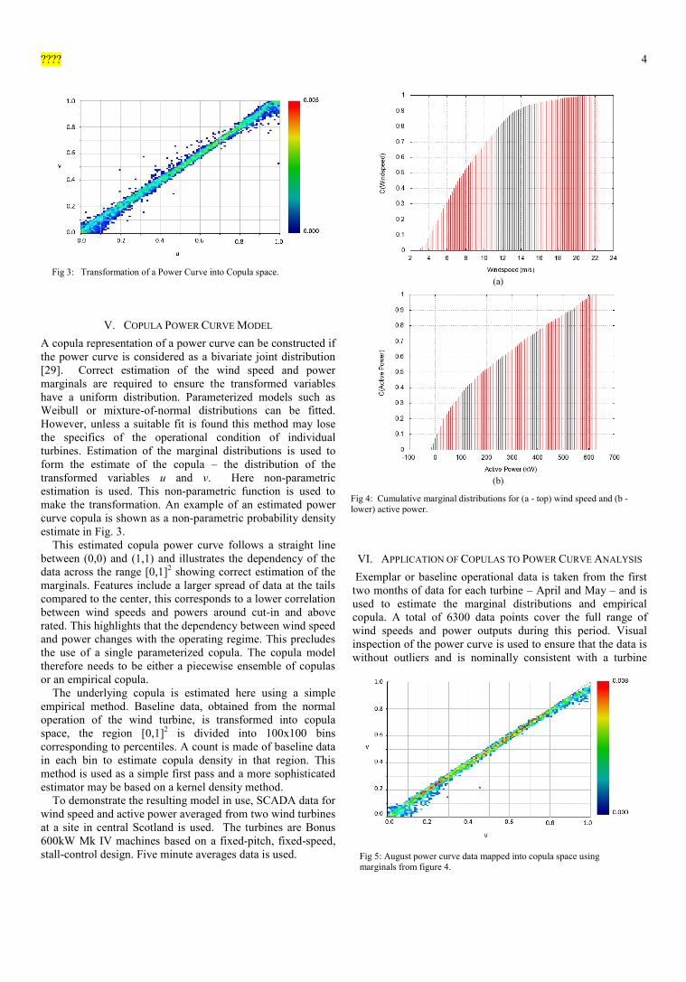
V. COPULA POWER CURVE MODEL

A copula representation of a power curve can be constructed ifthe power curve is considered as a bivariate joint distribution[29]. Correct estimation of the wind speed and powermarginals are required to ensure the transformed variableshave a uniform distribution. Parameterized models such asWeibull or mixture-of-normal distributions can be fitted.However, unless a suitable fit is found this method may losethe specifics of the operational condition of individualturbines. Estimation of the marginal distributions is used toform the estimate of the copula – the distribution of thetransformed variables u and v. Here non-parametricestimation is used. This non-parametric function is used tomake the transformation. An example of an estimated powercurve copula is shown as a non-parametric probability densityestimate in Fig. 3.

This estimated copula power curve follows a straight linebetween (0,0) and (1,1) and illustrates the dependency of thedata across the range [0,1]2 showing correct estimation of themarginals. Features include a larger spread of data at the tailscompared to the center, this corresponds to a lower correlationbetween wind speeds and powers around cut-in and aboverated. This highlights that the dependency between wind speedand power changes with the operating regime. This precludesthe use of a single parameterized copula. The copula modeltherefore needs to be either a piecewise ensemble of copulasor an empirical copula.

The underlying copula is estimated here using a simpleempirical method. Baseline data, obtained from the normaloperation of the wind turbine, is transformed into copulaspace, the region [0,1]2 is divided into 100x100 binscorresponding to percentiles. A count is made of baseline datain each bin to estimate copula density in that region. Thismethod is used as a simple first pass and a more sophisticatedestimator may be based on a kernel density method.

To demonstrate the resulting model in use, SCADA data forwind speed and active power averaged from two wind turbinesat a site in central Scotland is used. The turbines are Bonus600kW Mk IV machines based on a fixed-pitch, fixed-speed,stall-control design. Five minute averages data is used.

VI. APPLICATION OF COPULAS TO POWER CURVE ANALYSIS

Exemplar or baseline operational data is taken from the firsttwo months of data for each turbine – April and May – and isused to estimate the marginal distributions and empiricalcopula. A total of 6300 data points cover the full range ofwind speeds and power outputs during this period. Visualinspection of the power curve is used to ensure that the data iswithout outliers and is nominally consistent with a turbine

Fig 3: Transformation of a Power Curve into Copula space.(a)

(b)

Fig 4: Cumulative marginal distributions for (a - top) wind speed and (b -lower) active power.

Fig 5: August power curve data mapped into copula space usingmarginals from figure 4.

???? 5

operating correctly. Records with no output data are removedas it is assumed that the turbine is not operational at thesetimes. The cumulative probability density functions areestimated for the marginals by locating the percentile valuesand using linear interpolation. The cumulative densityfunctions for turbine 1 are shown in Fig. 4 (a) and (b).

The baseline data is transformed to the copula variablesaccording to:

Where w represents wind speeds and p is turbine poweroutput.

Data is binned in two dimensions as described in section V;the resulting copula density estimate is shown in Fig. 5. Itshould be noted that results show high joint probability closeto the u=v line with some variation in spread, the region inwhich data has greatest spread is at the tails. These areascorrespond to operation above rated wind speed at the top end,and the region around cut-in speed at the bottom.

To compare data from subsequent months, the estimatedmarginals, Fw and Fp, are used as transforms to map observeddata onto the empirical copula. The data for August istransformed and the resultant frequency distribution is shownin Fig. 5. During August readings corresponding to u<0.8appear to follow the estimated empirical copula. For u>0.8 thedata drops below the empirical copula. Fig. 6 shows theAugust data plotted as a power curve, with shading illustratingthe distribution of the baseline data. The drop in the Augustvalues of u and v can be seen to correspond to a smallreduction of power outputs for wind speed measured aboverated. This drop-off of data relative to the baseline is observedfor all months from July to October. Whilst this effect isrelatively small, it can have a significant effect on energygeneration across an extended period.

In order to compare operational data with baseline acrosstime periods or plant, three statistical measures of similarityare investigated. Since the original data is distributed about theu=v line with dissimilar data becoming increasingly distantfrom this two measured based on the sum-of-squared methodare proposed. The third measure based on a chi-squared typestatistic investigates the difference between the expected andmeasured number of data points within each binned region of

the copula.

A. Sum of Squares Similarity Estimation

As data sampled from the underlying copula should lay, withsome spread about the u=v line a simple statistic forcomparison is to sum either the residuals or the square of theresiduals relative to this line:

for analyzing a data set of n data pairs, (vi, ui) where for eachdata set the expected value of vi, that is , is given by thesimple equation u=v; this leads to the second equality in eachline. The two statistics R and R2 have different interpretations:R will stay close to 0 if the distribution is symmetrical aboutthe u=v line and will not detect changes in the variability ofthe data, it will however, detect data sets which deviate fromthe u=v line, for example the results in Fig. 5.The R2 statisticallows detection of changes to the variability of the data whilstsymmetry around the u=v line is maintained. This correspondsto a turbine showing higher variability of outputs across theoperating range. Data plotted on the empirical copula for anumber of months shows that performance often matchesbaseline throughout all the operating regimes except aboverated. As this corresponds to values of u greater thanapproximately 0.8 the R and R2 statistics are calculated bothfor entire range and the range u~[0.8,1]. Fig. 5 gives anexample of this.

B. Chi-squared Hypothesis TestA chi-squared style statistic can be used to test howappropriate a model is for a given data set. In this case howwell the test data is modeled by the estimated copula. Testdata for a particular month does not require the samemarginals as the baseline data, for example in a particularlywindy month they may be an excess of data at high u values.

pFvwFu pw11 ; (9)

n

uvn

vvR iiiii

ˆ (10)

2

2

2

22 ˆ

nuv

nvvR iiiii

(11)

Fig 6: August data plotted as power curve. Shading represents distributionof baseline data.

TABLE IACROSS FULL RANGE OF U

Month R (x10-2) R2 (x10-6) χ2 (x10-4)

June 0.201 0.579 2.95905July 1.32 1.36 1.419221

August 0.931 0.34 2.884236September 1.60 1.22 2.637837

October 0.845 1.17 2.10833November 0.459 0.726 2.218387December 0.571 0.713 4.893074

???? 6

To account for this the chi-squared statistic is constructed totest how well observed power-data fits the copula give windspeed measurements:

n

nEnO uiuivu2

2

(12)

Where Oi is the observed number of data points given the totalobserved points with the current u value summed over allv(nu). Ei is the expected number of data points given nu, and nis the total number of data points.

C. Application to case study data

The application of the copula analysis method is applied tocase study data. The method followed can be summarized by:

Step 1: Select baseline data; visual check to ensureconsistency

Step 2: Estimate marginals for wind speed and powerStep 3: Transform baseline data using estimated marginals

to produce empirical power curve copulaStep 5: Take new turbine data, transform using estimated

copulaStep 6: Use the statistics developed, R, R2 and χ2

Step 7: Do statistics show significant changes independency from baseline? If yes go to Step 8.Else go to step 9

Step 8: A change in power curve dependency has beenidentified – notify operators of possible fault/anomaly. Continue to Step 9.

Step 9: Take the next months data.

Tables I and II list the monthly R, R2, and χ2 values ascalculated for turbine 2 and plotted in Fig. 7. As noted above,turbine 2 showed signs of sub-optimal operation during themonths of July to October with the copula representationshowing a droop for high values of U (transformed windspeed).

Of the statistics analyzed, high R values occur during thesemonths. The difference is more pronounced for R across therestricted range (RU~[0.8,1]) . The other statistics do not, in this

case, provide a reliable signature that matches theobservations. It is anticipated that each statistic will be usefulin detecting specific fault modes as each will leave a particularsignature on the power curve dependency data. The possiblecorrelation between signatures and fault modes is discussed inthe next section.

As an example of a simple warning system, monthly data inwhich the value of RU~[0.8,1] ≥ 2 x 10-2 would provide a triggerfor operators of this turbine suggesting an incipient fault. Theparticular value of this limit will differ between turbines. Thecopula method outlined here provides a way of detectingchanges in the dependency between wind speed and power sowhilst 2 x 10-2 provides a useful value here, this is likely tovary between turbines depending on the specific locationconditions. For example if a turbine sees a higher turbulencelevel, the value of R is likely to be higher.

VII. DISCUSSION

The results from the previous section showed that the Copulaapproach has the ability to measure and identify changes independency between operationally measured wind speed andpower. These changes may be linked to specific faults, ormore gradual changes such as blade surface wear which ontheir own can lead to sub-optimal performance.

The correlation of faults or anomalies to statistical signaturesis key to developing copula-power curve conditionmonitoring. This initially would require detailed fault-logs and

TABLE IIACROSS U RANGE GREATER THAN 0.8 TO 1.0

Month R (x10-2) R2 (x10-6) χ2 (x10-4)

June 0.831 7.97 8.91July 5.0549 9.62 6.00

August 3.3389 12.9 7.68September 1.7741 3.12 6.73

October 3.2123 16.0 5.74November 1.7327 6.65 6.20December 0.0137 4.28 12.7

(a)

(b)

Fig 7: Monthly statistics for case study data including suggested warninglimits; upper (a) u~[0,1], lower (b) u~[0.8,1]

???? 7

regular, detailed manual inspection of turbines to provideinformation on issues like blade condition. Due to commercialsensitivities fault log data is often difficult to gain access to. Infact, many minor faults may go unnoticed and future work willneed to include more detailed observations of turbines.

This section provides some discussion on likely linksbetween the copula condition monitoring statistics and windturbine faults/anomalies. These may be difficult or impossibleto detect using current techniques and this section providessuggestions which the authors intend to continue in futurework.

Faults/anomalies will change the dependency between windspeed and power output and should therefore producesignatures in the R, R2 and χ2 statistics. Specific fault modeswill affect the turbine system in different ways socombinations of statistical signatures will be able to providesuggestions on the type of fault the turbine is experiencing.

A. Blade FaultsDegradation of the blade surface leads to a reduction in powerproduction as the turbine will have reduced aerodynamicallyefficient. The Copula-power curve will therefore lie below theu=v line. In stall regulated machines such as those studieshere, this is likely to effect the onset of stall and maycontribute to the sub-optimal performance identified here. The‘R’ statistic is likely to provide a good characterization of suchdeviations, and provide information on the direction of powerproduction variation.

Minor blade damage may not be detectable using the currentsensor systems attached to wind turbines, however even asmall reduction in aerodynamic efficiency can have asignificant effect on the profitability of a turbine. Here thechanges in dependency caused by gradual changes in thequality of the aerodynamic surfaces can be identified by theproposed copula method.

B. Yaw System FaultsThe yaw system attempts to maintain the turbine pointingdirectly into the wind. Misalignment leads to lowered airflowthrough the turbine and therefore lower power production.This will occur across the wind speed range. The effect islikely to be noticeable with a negative R value with thesignature appearing when calculated across the range u~[0,1].In addition to this signature the values of R2 and χ2 would beexpected to increase.

C. Pitch System FaultsMost modern turbines are pitch regulated. Below ‘rated

wind speed’ the blades pitch to the angle which allowsgreatest aerodynamic efficiency. With wind speed above ratedthe blades pitch to reduce the fraction of power transferredfrom the wind and to maintain rated power. Faulty pitchmechanisms are likely to show up through a greater variabilityat all wind speeds, or may lead to over or under production ofpower at high wind speeds. Increased variability will lead tohigher values of R2 and χ2

.The value of R is unlikely to providea clear signature as variability will occur above and below theu=v line.

These three fault modes provide a subset of all possiblefaults causing sub-optimal performance. The study of largerdata sets with more fault information will allow correlations tobe built up between copula statistics and faults. This providesa clear aim of future research.

Copula-power curve condition monitoring provides amethod of analyzing dependency data that can complementexisting condition monitoring methods. Whilst neural-networkanalysis of SCADA data typically studies correlations betweendata over the past two or three measurements, copula willallow comparison of dependencies over weeks, months orlonger. The use of copula methods to detect either minor faultsor performance degradation can be used to trigger more in-depth fault-analysis such as running physics based models tosuggest possible faults modes.

VIII. CONCLUSIONS

The application of copulas to wind turbine power curves hasbeen shown to allow analysis of the underlying dependencybetween wind speed and power; this paper has presented theexample of an empirical Copula tracking the non-linear andnon-stationary dependency between wind speed and activepower output from the SCADA data of two operational windturbines. Further developments may include the comparison,using copulas of the dependency from two or more turbines,and transforming data from one turbine using the marginaldistributions of another to allow comparison of the variabilityof data at different levels of production.

This work provides a first pass at Copula modeling for powercurves. A more sophisticated method of parametric estimationof marginals and dependency is required for the approach tobe maximally useful. This may take the form of a mixturedensity estimate of the marginals and a cubic spline estimateof the copula which would additionally capture and identifychanges in operating regime. Additionally, features withineach regime could be identified by the parameterization of themodel such as the variance over the gradient of the linear partof the curve which indicates the efficiency of the plant over itsuseful operating range of wind speeds, including the regionbetween rated wind speed and cut-out where the machine isoperating at full power. Piecewise application of Copulamodels to each of these regions may be sufficient to capturethese features of interest as local bivariate probabilitydensities.

REFERENCES

[1] DECC, The UK Renewable Energy Stratergy, DECC, Editor. 2009:London.

[2] European-Commission, Renewable Energy Road Map. Available:.http://europa.eu/legislation_summaries/energy/renewable_energy/l27065_en.htm (accessed 19th May 2011)

[3] Renewable energies in the 21st century: building a more sustainablefuture. 2006, European Commission. p. 21.

[4] DECC. A Prevailing Wind: Advancing UK Offshore WindDeployment, June 2009, London

[5] Wiggelinkhuizen, E.J., et al., Conmow - Final Report. 2007, EnergyResearch Center of the Netherlands.

[6] BERR, Scroby Sands Offshore Wind Farm 3rd Annual Report. 2007:London.

[7] Blanco, M.a.I., The economics of wind energy. Renewable andSustainable Energy Reviews, 2009. 13.

???? 8

[8] Tavner, P.J., J. Xiang, and F. Spinato, Reliability analysis for windturbines. Wind Energy, 2007. 10(1): pp. 1-18.

[9] Hahn, B., M. Durstewitz, and K. Rohrig, Reliability of Wind Turbines,in Wind Energy, J. Peinke, P. Schaumann, and S. Barth, Editors. 2007,Springer Berlin Heidelberg. pp. 329-332.

[10] Spinato, F., et al., Reliability of wind turbine subassemblies.Renewable Power Generation, IET, 2009. 3(4): pp. 387-401.

[11] Tavner, P.J., et al., Condition Monitoring of Rotating ElectricalMachines. 1 ed. Power and Energy Serries 2008, Stevenage: TheInstitue of Engineering and Technology.

[12] IEC 61400:,Wind Turbine Genertor Systems, Part 12: Wind TurbinePower Performace Testing. 1998.

[13] Kusiak, A. Zheng, H. Song, Z. On-line Monitoring of Power Curves.Renewable Energy, 2009. 34. pp. 1487 – 1493.

[14] Hameed, Z., et al., Condition monitoring and fault detection of windturbines and related algorithms: A review. Renewable and SustainableEnergy Reviews, 2009. 13(1): pp. 1-39.

[15] Crabtree, C.J., Survey of commercially Available ConditionMonitoring Systems for Wind Turbines. 2010, Durham University;SuperGen Wind.

[16] Gray, C.S. and S.J. Watson, Physics of Failure approach to windturbine condition based maintenance. Wind Energy 13(5): pp. 395-405. Wiley 2010.

[17] Rodriguez, L., et al. Application of latent nestling method usingColoured Petri Nets for the Fault Diagnosis in the wind turbinesubsets. in Emerging Technologies and Factory Automation, 2008.ETFA 2008. IEEE International Conference on. 2008.

[18] Zaher, A., et al., Online wind turbine fault detection throughautomated SCADA data analysis. Wind Energy, 2009. 12(6): pp. 574-593.

[19] A. Kusiak and W.Y. Li, The Prediction and Diagnosis of WindTurbine Faults, Renewable Energy, Vol. 36, No. 1, pp. 16-23, 2011.

[20] Leaney, V., C;, D. Sharpe, J;, and D.G. Infield, Condition MonitoringTechniques for Optimisation of Wind Farm Performance.International Journal of Comaden, 1999. 2(1).

[21] Xiang, Y., et al. Unsupervised learning and fusion for failure detectionin wind turbines. in Information Fusion, 2009. FUSION '09. 12thInternational Conference on. 2009.

[22] Garcia, M.C., M.A. Sanz-Bobi, and J. del Pico, SIMAP: IntelligentSystem for Predictive Maintenance: Application to the healthcondition monitoring of a windturbine gearbox. Computers in Industry57(6): pp. 552-568, Elsevier 2006.

[23] R. Duda, P. Hart and D. Stork, “Pattern Classification” 2nd EditionWiley-Interscience, 2001.

[24] Sklar, A., Fonctions de repartition a n dimensions et leurs marges.Publ. Inst. Statist. Univ. Paris, 1959. 8: pp. 229-231.

[25] R.B. Nelsen. "An Introduction to Copulas", 2nd Edition. SpringerSeries in Statistics, 2006.

[26] Patton, A.J., Modelling asymmetric exchange rate dependence.International Economic Review, 2006. 47(2): pp. 527-556.

[27] Berks, P., F. Wood, and J. Pillow, Characterizing NeuralDependencies with Coupla Models. Advances in Neural InformationProcessing Systems 2009. 21: pp. 129-136.

[28] L, R., On the distribution transform, Sklar's Theorem, and theempirical copula process. J. Statist. Plan. Infer, 2009. 139(11): pp.3921-3927.

[29] Stephen, B.; Galloway, S. J.; McMillan, D.; Hill, D. C.; Infield, D. G.;“A Copula Model of Wind Turbine Performance”, IEEE Transactionson Power Systems 26 2, pp. 965 – 966, 2011.

Simon Gill is currently a PhD candidate within the WindEnergy Doctoral Training Centre at the University ofStrathclyde. He obtained a Masters degree in Astrophysicsfrom the University of Edinburgh in 2003, followed by aPGCE in secondary science education in 2005. His researchinterests include active management of distribution networksand the integration of renewable energy into power systems.

Dr Bruce Stephen currently holds the post of SeniorResearch Fellow within the Institute for Energy andEnvironment at the University of Strathclyde. He received hisB.Sc. from Glasgow University and M.Sc. and PhD degreesfrom the University of Strathclyde. His research interestsinclude Distributed Information Systems, Machine Learning

applications in Power System and Animal Welfare Condition Monitoring andAsset Management.

Dr Stuart Galloway is a Senior Lecturer within the Institutefor Energy and Environment. He obtained his MSc and PhDdegrees in mathematics from the University of Edinburgh in1994 and 1998 respectively. His research interests includepower system optimization, numerical methods andsimulation of novel electrical architectures.