winter 2010
DESCRIPTION
Winter 2010. Macroeconomics. Starring Erik Hurst. Some Perspective: Major Historical Recessions. Economic Recoveries. The question at hand: When will we return to “normal growth?” Note:Out of a recession does not mean normal growth “V” shape recoveries (rapid growth out of a recession) - PowerPoint PPT PresentationTRANSCRIPT
Winter 2010Winter 2010
MacroeconomicsMacroeconomics
Starring Erik Hurst
1

2
Some Perspective: Major Historical Recessions

3
Economic Recoveries
The question at hand: When will we return to “normal growth?”
Note: Out of a recession does not mean normal growth
• “V” shape recoveries (rapid growth out of a recession)
• “U” shape recoveries (sluggish growth before recovery)
• “W” shape recoveries (slip back into another recession)
• “Reverse J” shape recoveries (sluggish growth to lower level)
4
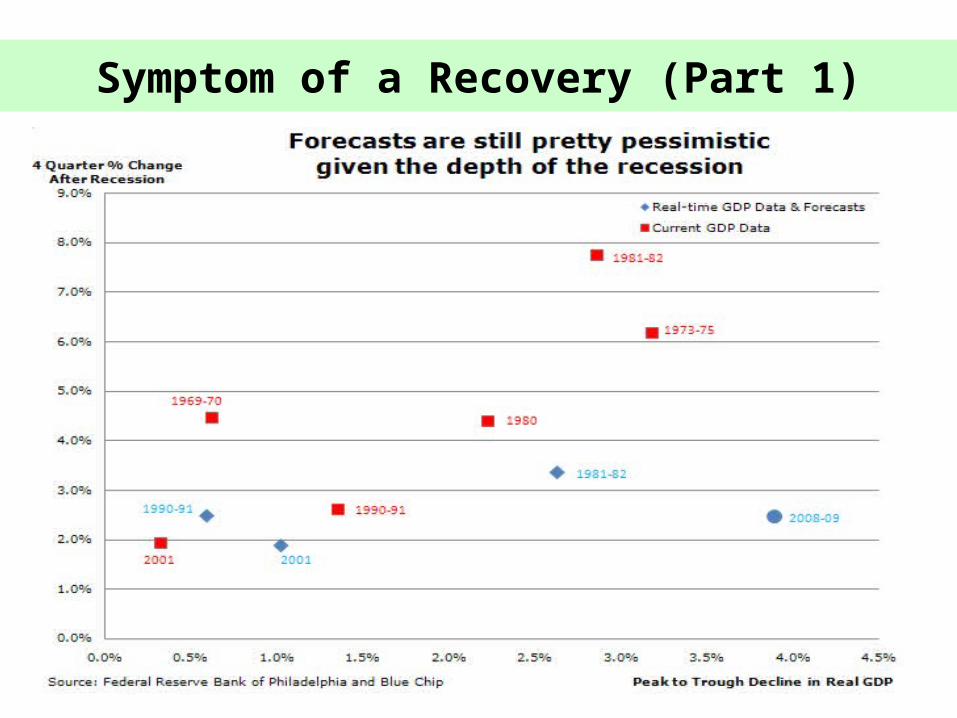
Symptom of a Recovery (Part 1)

5
Symptom of a Recovery (Part 2)
Real Gross Domestic Product: Quarterly, 1970Q1 – 2009Q3
Note: The black line is the level of real GDP (left axis)
Note: The red line is quarter over quarter growth rates of real GDP (right axis)

6
Symptom of Recession (Part 3)
U.S. Consumption Expenditures: Quarterly, 1970Q1 – 2009Q3

7
Symptom of Recession (Part 4)
Consumer Sentiment: Monthly, 1978M1 – 2009M10

8
Symptoms of a Recovery (Part 5)
Unemployment Rate: Monthly 1970M1 – 2009M10

9
Consensus of State of the Economy
• The recession likely over.
• The million dollar question: what will the recovery look like?
• Has the U.S. macroeconomic landscape changed?
• What will economic growth look like going forward.
10
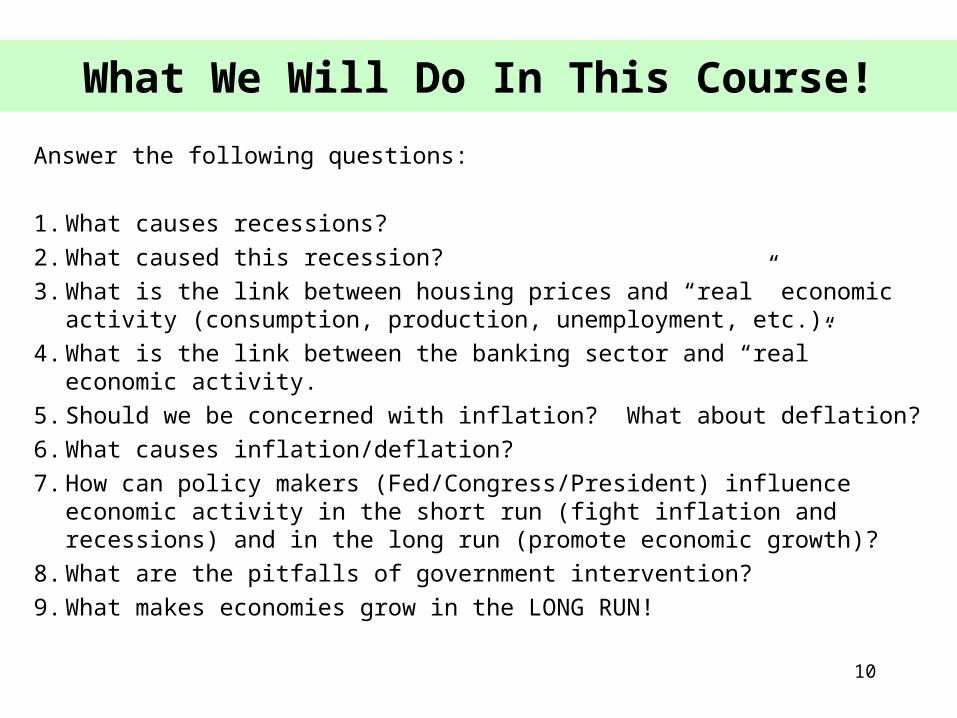
What We Will Do In This Course!
Answer the following questions:
1. What causes recessions?
2. What caused this recession?
3. What is the link between housing prices and “real” economic activity (consumption, production, unemployment, etc.).
4. What is the link between the banking sector and “real” economic activity.
5. Should we be concerned with inflation? What about deflation?
6. What causes inflation/deflation?
7. How can policy makers (Fed/Congress/President) influence economic activity in the short run (fight inflation and recessions) and in the long run (promote economic growth)?
8. What are the pitfalls of government intervention?
9. What makes economies grow in the LONG RUN!

11
What We Will Do In This Course!
Some additional topics we will cover along the way….:
• What makes consumers “consume”?
• Do consumers save too little?
• Why are banks currently hoarding cash?
• What is the role of “uncertainty” on economic activity?
• What issues must we confront with Social Security?
• Why can government budget deficits be bad?
• Should the Federal Reserve be abolished (or changed)?
• Does it make sense to put controls on labor markets (minimum wage laws, maximum wage laws (salary caps), etc.)?
• What effect do taxes have on the U.S. economy in the short run and the long run?
• What is the link between the world economy and the U.S. economy?

12
A Caveat
• My course takes the perspective of analyzing any large macroeconomy (with respect to the models we build).
• The examples will come from the U.S. (because that is what I study)
• However, the insights apply equally well to all large developed economies including:
– The European Union
– Japan
– Canada, Australia, etc. (for the most part).
• The models also explains well consumer, business, and government behavior for all economies (China, India, etc.).

13
Course Preliminaries
• Course Schedule We have 11 sessions this quarter (see syllabus)
• Quizzes: 8 quizzes (see syllabus)Drop 2 lowest quizzes.All quizzes will take place at the start of class.NEVER – EVER – Give Makeup Quizzes/Midterm
• Midterm: Midterm during week 5 (session 6). It is optional.

14
Course Preliminaries
• Grading Policy: 30% quizzes, 70% midterm and final.
• Readings/Must Reads: Assigned (encouraged). I will try to link to lectures.
• “Readings are Fair Game For All Quizzes and Tests”
• Each week, I will send out a weekly email update stating what readings you will be responsible for during the subsequent quiz.
• Be patient – this is a course that builds a model of the macroeconomy – the payoff comes once the model is built (lecture 7ish).

TOPIC 1TOPIC 1
A Introduction to Macro DataA Introduction to Macro Data
15

16
Goals of the Lecture
• What is Gross Domestic Product (GDP)? Why do we care about it?
• How do we measure standard of livings over time?
• What are the definitions of the major economic expenditure components?
• What are the trends in these components over time?
• What is the difference between ‘Real’ and ‘Nominal’ variables?
• How is Inflation measured? Why do we care about Inflation?
• How is Unemployment measured? Why do we care about Unemployment?
• What have been the predominant relationships between Unemployment, Inflation and GDP over the last four decades.
NOTE: This lecture will likely go into next week. This is by design. It does not mean we will be short changed on other material later in the class.

17
Gross Domestic Product (GDP)
• GDP is a measure of output!
• Why Do We Care?
– Because output is highly correlated (at certain times) with things we care about (standard of living, wages, unemployment, inflation, budget and trade deficits, value of currency, etc…)
• Formal Definition:
– GDP is the Market Value of all Final Goods and Services Newly Produced on Domestic Soil During a Given Time Period (different than GNP)

18
“Production” Equals “Expenditure”
• GDP is a measure of Market Production!
• GDP = Expenditure = Income = Y (the symbol we will use)
(in macroeconomic equilibrium)
• What is produced in the market has to be show up as being purchased or held by some economic agent;
• Who are the economic agents we will consider on the expenditure side?
– Consumers (refer to expenditure of consumers as “consumption”)
– Businesses (refer to expenditure of firms as “investment”)
– Governments (refer to expenditures of governments as “government spending”)
– Foreign Sector (refer to expenditures of foreign sector as “exports”)

19
A Simple Example
• What is “produced” has to be “purchased” by someone (including the producer).
• Suppose I produce silverware (forks, spoons, etc.). If so, I could:
– sell it to some domestic customer (Consumption)
– sell it some business (Investment)
– keep it in my stock room as inventory (Investment)
– sell it to the city of Chicago to use in their shelters (Government spending)
– sell it to some foreign customer (Export)

20
“Production” Equals “Income”
• What is Produced is Also a Measure of Income.
• If you pay a $1 for something, that $1 has to end up in someone’s pocket as:
Wages/Salary (compensation for workers who make production)
Profits (compensation for self employed)
Rents (compensation for land owners)
Interest (compensation for debt owners)
Dividends (compensation for equity owners)
• Notice, wages are only one component of income (Y does not equal wages)! (Although, under certain production functions, they will be proportional to each other).
21
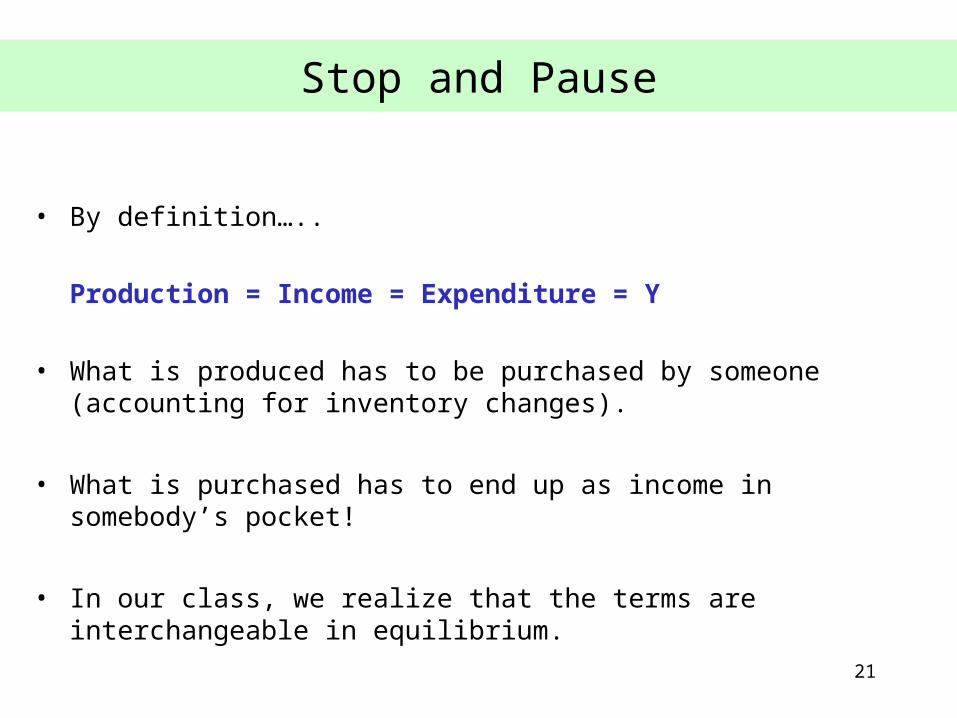
Stop and Pause
• By definition…..
Production = Income = Expenditure = Y
• What is produced has to be purchased by someone (accounting for inventory changes).
• What is purchased has to end up as income in somebody’s pocket!
• In our class, we realize that the terms are interchangeable in equilibrium.
22
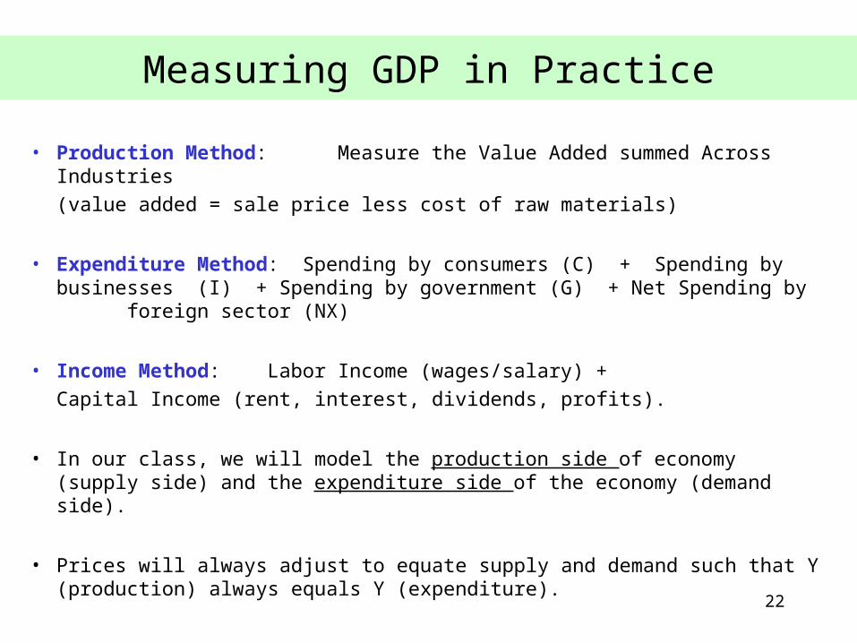
Measuring GDP in Practice
• Production Method: Measure the Value Added summed Across Industries
(value added = sale price less cost of raw materials)
• Expenditure Method: Spending by consumers (C) + Spending by businesses (I) + Spending by government (G) + Net Spending by foreign sector (NX)
• Income Method: Labor Income (wages/salary) +
Capital Income (rent, interest, dividends, profits).
• In our class, we will model the production side of economy (supply side) and the expenditure side of the economy (demand side).
• Prices will always adjust to equate supply and demand such that Y (production) always equals Y (expenditure).

23
What GDP is NOT!
• GDP is not, or never claims to be, an absolute measure of well-being!
– Size effects : But even GDP per capita is not a perfect measure of welfare
• “The gross national product does not allow for the health of our children, the quality of their education, or the joy of their play. It does not include the beauty of our poetry or the strength of our marriages, the intelligence of our public debate or the integrity of our public officials. It measures neither our courage, nor our wisdom, nor our devotion to our country. It measures everything, in short, except that which makes life worthwhile, and it can tell us everything about America except why we are proud to be Americans.”
– U.S. Senator Robert F. Kennedy, 1968
24
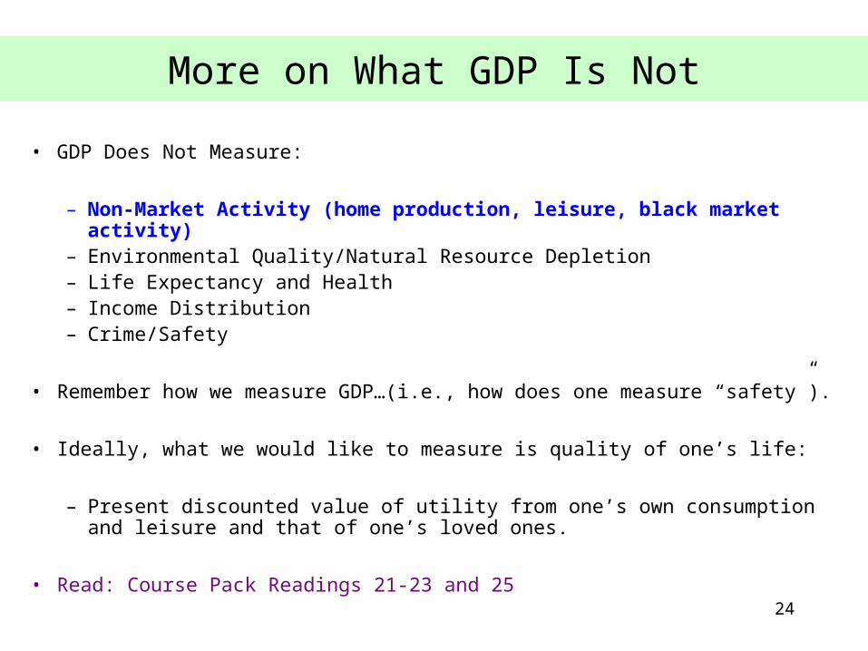
More on What GDP Is Not
• GDP Does Not Measure:
– Non-Market Activity (home production, leisure, black market activity)– Environmental Quality/Natural Resource Depletion– Life Expectancy and Health– Income Distribution– Crime/Safety
• Remember how we measure GDP…(i.e., how does one measure “safety”).
• Ideally, what we would like to measure is quality of one’s life:
– Present discounted value of utility from one’s own consumption and leisure and that of one’s loved ones.
• Read: Course Pack Readings 21-23 and 25

25
Defining the Expenditure Components (formally)
• Consumption (C):
– The Sum of Durables, Non-Durables and Services Purchased Domestically by Non-Businesses and Non-Governments (ie, individual consumers).
– Includes Haircuts (services), Refrigerators (durables), and Apples (non-durables).– Does Not Include Purchases of New Housing.
• Investment (I):
– The Sum of Durables, Non-Durables and Services Purchased Domestically by Businesses
– Includes Business and Residential Structures, Equipment and Inventory Investment– Land purchases are NOT counted as part of GDP (land is not produced!!)– Stock purchases are NOT counted as part of GDP (stock transactions do NOT
represent production – they are saving!)
There is a difference between financial and economic investment!!!!!!!

26
More On Expenditure/Production Components
• Government Spending (G): Goods and Services Purchased by the domestic government.
• For the U.S., 2/3 of this is at the state level (police and fire protection, school teachers, snow plowing) and 1/3 is at the federal level (President, Post Office, Missiles).
• NOTE: Welfare and Social Security are NOT Government Spending. These are Transfer Payments. Nothing is Produced in this Case.
• Net Exports (NX): Exports (X) - Imports (IM); – Exports: The Amount of Domestically Produced Goods Sold on Foreign Soil – Imports: The Amount of Goods Produced on Foreign Soil Purchased
Domestically.

27
Summary of the Demand Side of Economy
• Expenditures:
Y = C + I + G + X - IM
• Only four economic agents can “spend” on domestic production
Domestic consumers (C)
Domestic firms (I)
Domestic governments (G)
Foreign consumers, firms, and governments (X)
• We will develop models for each sub component of the expenditure side of the economy (C, I, G, and NX).
28
Measuring Expenditure (Demand Side)
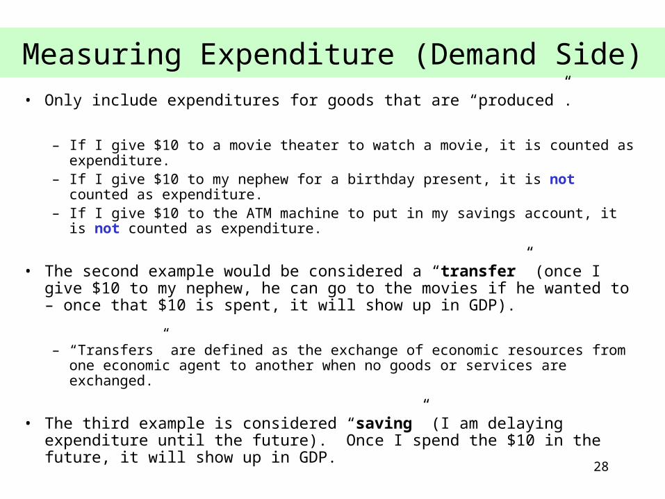
• Only include expenditures for goods that are “produced”.
– If I give $10 to a movie theater to watch a movie, it is counted as expenditure.– If I give $10 to my nephew for a birthday present, it is not counted as expenditure.– If I give $10 to the ATM machine to put in my savings account, it is not counted as
expenditure.
• The second example would be considered a “transfer” (once I give $10 to my nephew, he can go to the movies if he wanted to – once that $10 is spent, it will show up in GDP).
– “Transfers” are defined as the exchange of economic resources from one economic agent to another when no goods or services are exchanged.
• The third example is considered “saving” (I am delaying expenditure until the future). Once I spend the $10 in the future, it will show up in GDP.
29
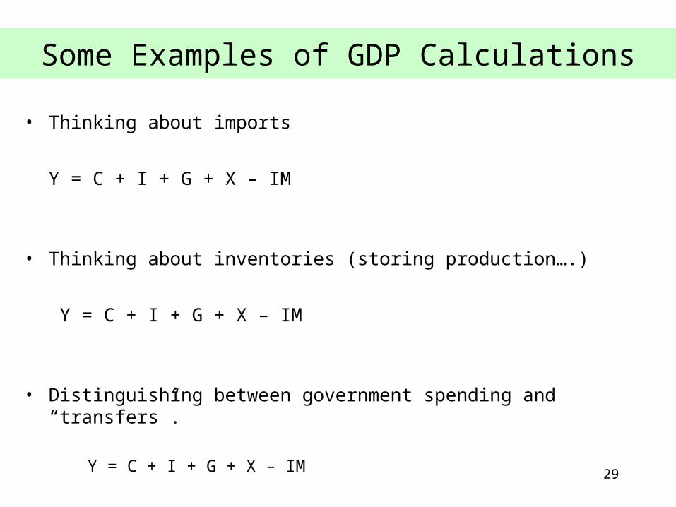
Some Examples of GDP Calculations
• Thinking about imports
Y = C + I + G + X – IM
• Thinking about inventories (storing production….)
Y = C + I + G + X – IM
• Distinguishing between government spending and “transfers”.
Y = C + I + G + X – IM
30
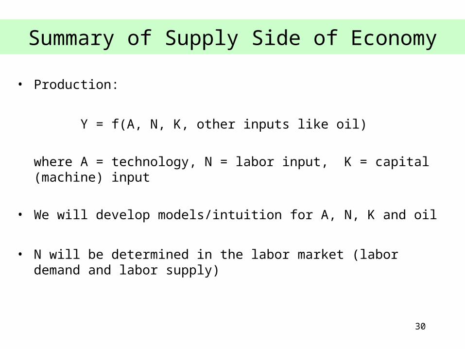
Summary of Supply Side of Economy
• Production:
Y = f(A, N, K, other inputs like oil)
where A = technology, N = labor input, K = capital (machine) input
• We will develop models/intuition for A, N, K and oil
• N will be determined in the labor market (labor demand and labor supply)

31
Where We are Headed
32
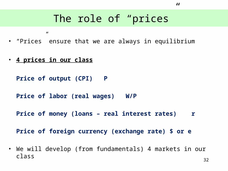
The role of “prices”
• “Prices” ensure that we are always in equilibrium
• 4 prices in our class
Price of output (CPI) P
Price of labor (real wages) W/P
Price of money (loans – real interest rates) r
Price of foreign currency (exchange rate) $ or e
• We will develop (from fundamentals) 4 markets in our class

33
The 4 Markets
1) Labor Demand vs. Labor Supply (determines N and W/P)
Necessary to compute the supply side of economy
Key to where recessions come from (frictions in the labor market)
2) IS-LM market (determines r and Y (via I))
Interest rates determine firm investment
Key to federal reserve policy (sets r)
Key to understanding banking crises.
3) Aggregate Demand vs. Aggregate Supply (determines P and Y)
Key to understanding where inflation comes from!

34
The 4 Markets (continued)
4) Foreign Exchange Market (determines value of currency and NX)
We will focus on this market in week 10
Notice, markets 1-3 help to pin down the level of Y in the economy
These four markets (and their components) will determine everything we want to know about the macroeconomy (production, inflation, economic growth, unemployment, interest rates, budget deficits, trade deficits, etc.)
For the next 7 weeks, we will build the underpinnings of these markets. In doing so, we will uncover how these markets work and what factors influence those markets!

35
An Important Equation
36
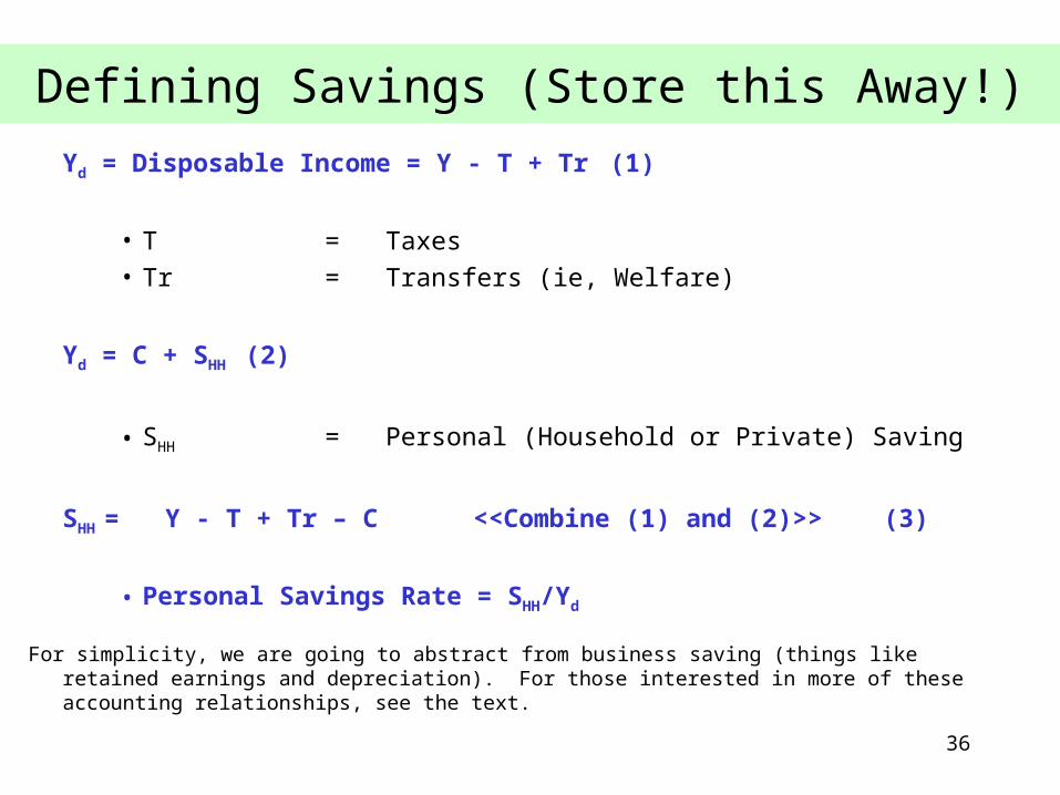
Defining Savings (Store this Away!)
Yd = Disposable Income = Y - T + Tr (1)
• T = Taxes
• Tr = Transfers (ie, Welfare)
Yd = C + SHH (2)
• SHH = Personal (Household or Private) Saving
SHH = Y - T + Tr – C <<Combine (1) and (2)>> (3)
• Personal Savings Rate = SHH/Yd
For simplicity, we are going to abstract from business saving (things like retained earnings and depreciation). For those interested in more of these accounting relationships, see the text.

37
A Look at Actual U.S. Household Saving Rates: 1970Q1 – 2009Q3
Note: Shaded areas are recessions.

38
Saving Identities (continued)
Sgovt = T - (G + Tr) (4)
• Sgovt = Government (Public) Saving
• Includes Federal, State and Local Saving
• What government collects (T) less what they pay out (G and Tr)
S = SHH + Sgovt = Y - C - G = I + NX (5)
• S = National Savings
so,
S = Y - C – G <<Combine (3) and (5)>> (6)
S = I + NX <<Combine (6) and Y = C+I+G+NX>> (7)

39
Summary
S = I + NX
We will use this equation for the rest of the class!
National savings, goes into a “bank”.
Firms looking to borrow, go to the “bank”.
Firms can only borrow what is in the “bank”
In a world where NX = 0, interest rates will adjust such that savings will always equal investment (I=S – this will be our IS curve later in the course).
What is the role of NX? (International savings)
40
Understanding Prices and Inflation

41
Prices and Inflation
• Inflation rate = % change in P, where P is the level of Prices
• [P(t+1) - P(t)] / P(t)
• How Are Prices Measured?
• Price Indexes – a relative measure of a ‘basket’ of many goods
• GDP Deflator (one prominent price index):
Value of Current Output at Current Prices / Value of Current Output at Base Year Prices
• Another prominent price index is the CPI (consumer price index) – measures price changes of consumer goods. I will often use the CPI as our measure of a price index in this class.
42
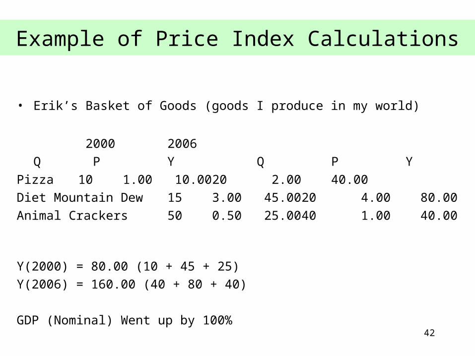
Example of Price Index Calculations
• Erik’s Basket of Goods (goods I produce in my world)
2000 2006
Q P Y Q P Y
Pizza 10 1.00 10.00 20 2.00 40.00
Diet Mountain Dew 15 3.00 45.00 20 4.00 80.00
Animal Crackers 50 0.50 25.00 40 1.00 40.00
Y(2000) = 80.00 (10 + 45 + 25)
Y(2006) = 160.00 (40 + 80 + 40)
GDP (Nominal) Went up by 100%

43
Example of Price Index Calculation (Continued)
• Nominal GDP is output valued at Current Prices• Comparing Nominal GDPs over time can become problematic
– Confuse Changes in Output (production) with Changes in Prices
• Real GDP is output valued at some Constant Level of Prices (prices in a base year).
Real GDP(t) = Nominal GDP(t) / Price Index (t)
• Growth in Real GDP:
% Δ in Real GDP = [Real GDP (t+1) - Real GDP (t)]/Real GDP (t)
or (approximately)
% Δ in Real GDP = % Δ in Nominal GDP - % Δ in P
44
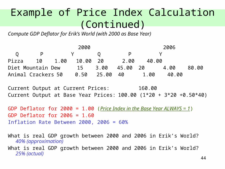
Example of Price Index Calculation (Continued)
Compute GDP Deflator for Erik’s World (with 2000 as Base Year)
2000 2006Q P Y Q P Y
Pizza 10 1.00 10.00 20 2.00 40.00Diet Mountain Dew 15 3.00 45.00 20 4.00 80.00Animal Crackers 50 0.50 25.00 40 1.00 40.00
Current Output at Current Prices: 160.00Current Output at Base Year Prices: 100.00 (1*20 + 3*20 +0.50*40)
GDP Deflator for 2000 = 1.00 (Price Index in the Base Year ALWAYS = 1)GDP Deflator for 2006 = 1.60 Inflation Rate Between 2000, 2006 = 60%
What is real GDP growth between 2000 and 2006 in Erik’s World? 40% (approximation)What is real GDP growth between 2000 and 2006 in Erik’s World? 25% (actual)

45
Technical Notes on Price Indexes
• Need to Pick a Basket of Goods (cannot measure all prices)
• ‘Ideal/Representative’ Basket of Goods Change Over Time
– Invention (Computers, Cell Phones, VCRs, DVDs).
– Quality Improvements (Anti-Lock Brakes)
• Criticism of Price Indices: Part of the Change in Prices Represents a Change in Quality - Actually, not measuring the same goods in your basket over time.
• How do we account for “sales”?
• Additionally - technology advances drive down the price of ‘same’ goods over time.

46
Technical Notes on Price Indexes
• Boskin Report (1996) Concludes that CPI Overstates Inflation by 1.1% per year.
• Overstating Inflation means understated Real GDP increases - makes it appear that the U.S. Economy has Grown Slower Over Time. (Same for Stock Market, Housing Prices, Wages - any Nominal Measure).
• Measures to Get Around Problems with CPI - Chain Weighting – Read Text to get a sense of chain weighting.
• Read Course Pack Readings: 20 (difficulty measuring prices)

47
Technical Notes on Price Indexes
• Which is better: Real or Nominal?
– In this class, we will focus on the ‘Real’! We are trying to measure changes in production, expenditures, income, standard of livings, etc. We will separately focus on the changes in prices.
– From now on, both in the analytical portions and the data portions of the course, we will assume everything is real unless otherwise told.
• ie, Y = Real GDP, C = Real Consumption, G = Real Government Purchases, etc...

48
A Look at U.S. Nominal GDP: 1970Q1 – 2009Q3
Black line - trend in nominal GDP over time (left axis)Red line - trend in nominal GDP growth (percentage change in nominal GDP) over time(right axis) (growth measured year over year)Shaded areas represent “official” recession dates (as calculated by National Bureau of Economic Research)

49
A Look at U.S. Inflation 1970M1 - 2009M11
Black line - trend in CPI over time (left axis)Red line - trend in CPI inflation rate (percentage change in CPI) over time (right axis) (growth measured year over year)
Shaded areas represent “official” recession dates (as calculated by National Bureau
of Economic Research)
50
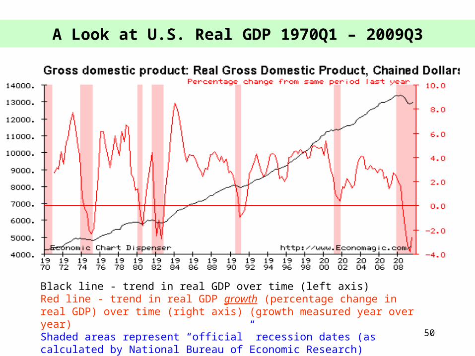
A Look at U.S. Real GDP 1970Q1 – 2009Q3
Black line - trend in real GDP over time (left axis)Red line - trend in real GDP growth (percentage change in real GDP) over time (right axis) (growth measured year over year)Shaded areas represent “official” recession dates (as calculated by National Bureau of Economic Research)

51
Recessions and Inflation in U.S. Over Last 40 Years

52
Real GDP and Inflation Over the Last Three Decades?
High or Rising Inflation: 73-75 07-0879-80
Low or Falling Inflation: 81-83 96-00 (sustained) 08-09
90-91 01-02
High Growth in GDP: 83-8696-00 (sustained)
Negative Growth in GDP: 74-75 90-9179-80 01-0281-83 08-09
1) Sometimes Negative Growth in GDP and Rising Inflation (70s)2) Sometimes Negative Growth in GDP and Falling Inflation (80s and 90s)
Need Theory to Explain Both Sets of Facts!!!!

53
What is a Recession?
• “Official Rule of Thumb” - 2 or more quarters of negative real GDP growth
• Most Economies are usually not in recession
– U.S. average postwar expansion: 50 months
– U.S. average postwar recession: 11 months
– Previous Recession: 7-9 months (April 2001 – December 2001)
– Previous Expansion: 121 months (March 1991- March 2001)
– The 1990s experienced the longest expansion since 1850 (the second longest was 106 months ; 1961-1969)
– For Information on Business Cycle Dates see: http://www.nber.org/cycles.html
54
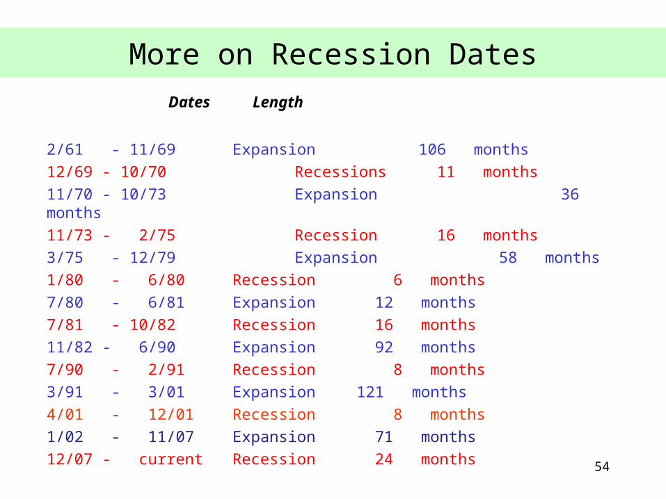
More on Recession Dates
Dates Length
2/61 - 11/69 Expansion 106 months
12/69 - 10/70 Recessions 11 months
11/70 - 10/73 Expansion 36 months
11/73 - 2/75 Recession 16 months
3/75 - 12/79 Expansion 58 months
1/80 - 6/80 Recession 6 months
7/80 - 6/81 Expansion 12 months
7/81 - 10/82 Recession 16 months
11/82 - 6/90 Expansion 92 months
7/90 - 2/91 Recession 8 months
3/91 - 3/01 Expansion 121 months
4/01 - 12/01 Recession 8 months
1/02 - 11/07 Expansion 71 months
12/07 - current Recession 24 months

55
Great Moderation?
Dates Length
2/61 - 11/69 Expansion 106 months
12/69 - 10/70 Recessions 11 months
11/70 - 10/73 Expansion 36 months
11/73 - 2/75 Recession 16 months
3/75 - 12/79 Expansion 58 months
1/80 - 6/80 Recession 6 months
7/80 - 6/81 Expansion 12 months
7/81 - 10/82 Recession 16 months
11/82 - 6/90 Expansion 92 months
7/90 - 2/91 Recession 8 months
3/91 - 3/01 Expansion 121 months
4/01 - 12/01 Recession 8 months
1/02 - 11/07 Expansion 71 months
12/07 - current Recession 24 months
16 months of recession in24 years (1982-2007)
49 months of recession in 21 years (1961-1982)
The Great Moderation
56
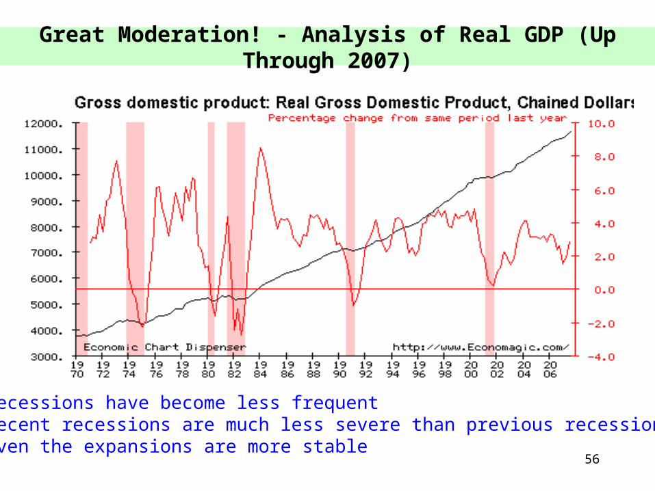
Great Moderation! - Analysis of Real GDP (Up Through 2007)
• Recessions have become less frequent • Recent recessions are much less severe than previous recessions • Even the expansions are more stable

57
Is the Great Moderation Dead?
• I do not think so….
My interpretation:
Great Moderation refers to the fact that the economy is better at minimizing the impact of any given shock now relative to 30 years ago.
It does not mean that:
There will not be bad shocksThere will not be “new” shocks
Why? The economy is more flexible (inventory management, credit)We have gotten better at conducting macroeconomic policy!
58
Foreshadowing the rest of the course
• Assume aggregate demand (drawn in {Y,P} space) slopes down
I will prove this to you later in the course
• Assume short run aggregate supply (drawn in {Y,P} space) slopes up
I will prove this to you later in the courseI will also distinguish between short run and long run aggregate supply

59
Foreshadowing the Rest of the Course: Demand Shocks
The relationship between inflation and output when aggregate demand shifts:
Suppose we are in long run equilibrium at point (a) (AD = SRAS = LRAS)
Y
Short Run AS
AD
Long Run AS
Y*
P
AD’
a
b
Y’
P’P
If the economy receives a negative aggregate demand shock, short run equilibrium will move from point (a) to point (b). Output will fall (from Y* to Y’). Prices will fall (from P to P’).
Demand shocks cause prices and output to move in the same direction.(You should be able to illustrate a positive demand shock)
60
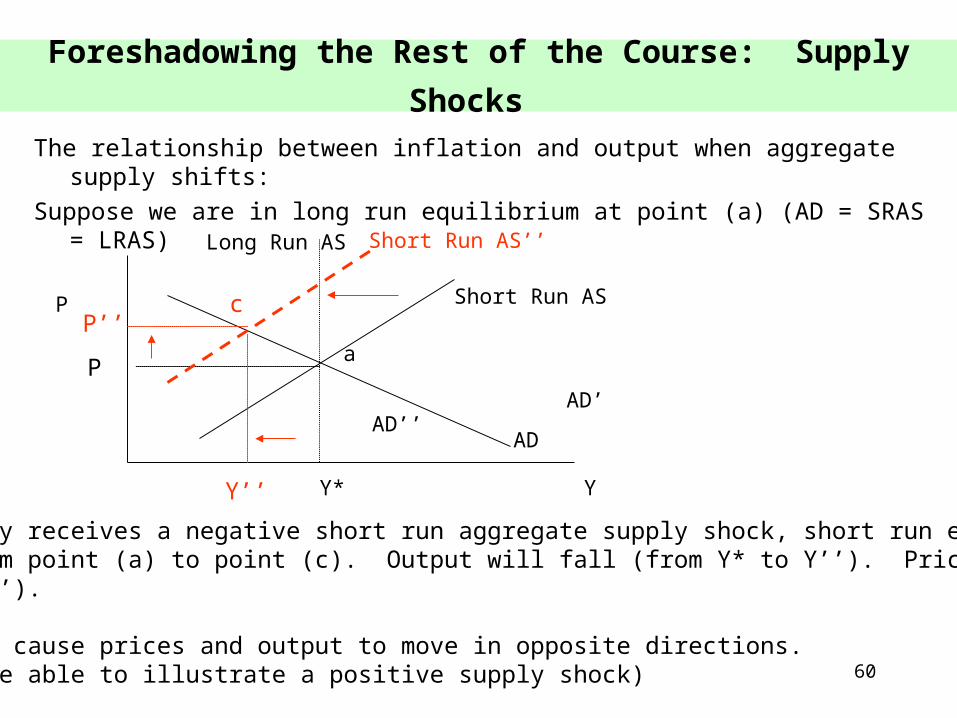
Foreshadowing the Rest of the Course: Supply Shocks
The relationship between inflation and output when aggregate supply shifts:
Suppose we are in long run equilibrium at point (a) (AD = SRAS = LRAS)
Y
Short Run AS
AD
Long Run AS
Y*
P
AD’AD’’
a
Y’’
P’’
P
Short Run AS’’
c
If the economy receives a negative short run aggregate supply shock, short run equilibrium will move from point (a) to point (c). Output will fall (from Y* to Y’’). Prices will rise (from P to P’’).
Supply shocks cause prices and output to move in opposite directions.(You should be able to illustrate a positive supply shock)

61
Reinterpreting the Business Cycle Data 1970-2008
1970 recessions: Inflation increasing at start of recession! (supply shock)
(cause: rapidly rising oil prices)
1981 recession: Dramatic decrease in inflation at start of recession (demand shock) (cause: Fed induced recession)
1990 recession: Slight decline in inflation at start of recession (demand shock) (cause: fall in consumer confidence/oil
price increase)
1990s rapid growth: No inflation (supply shock)
(cause: IT revolution)
2001 recession: A fall in inflation (demand shock)
(cause: over confidence by firms: inventory adjustment)
2008 recession: An increase in inflation (supply shock – oil prices) and then a fall in inflation (demand shock – housing/banking crises)

62
Business Cycles vs. Long Run Growth

63
Macroeconomic Goals
Promote Economic Growth
Minimize uncertainty
Minimize distortions in the economy (create level playing field)
Create incentives for efficient economic transactions
Maximize “trend” growth
Promote Economic Stability
Keep the unemployment rate low
Keep inflation in check
Refer to this as managing “business cycles” – minimize the deviations (cycles) around the trend.
Lower uncertainty leads to greater economic activity

64
Why We Care About Inflation and Unemployment

65
Interest Rates
i0,1 = the nominal interest rate between periods 0 and 1
(the nominal return on the asset)
πe0,1 = the expected inflation rate between periods 0 and 1
re0,1 = the expected real interest rate between periods 0 and 1
Definitions
re0,1 = i0,1 - πe
0,1 (or i0,1 = πe0,1 + re
0,1)
ra0,1 = i0,1 - πa
0,1 (or i0,1 = πa0,1 + ra
0,1)
where ra and πa are the actual real interest rate and inflation

66
Interest Rate Notes
• The Formula given is approximate. The approximation is less accurate the higher the levels of inflation and nominal interest rates. The exact formula is re = (1 + i) / (1 + лe) - 1
• Central Banks are very interested in r since it may affect the savings decisions of households and definitely affects the investment decisions of firms. The press talks about Central Banks setting i, but the Central Banks are really trying to set r.
• 3 easy ways of measuring expected inflation:– Recent actual inflation (see http://www.clev.frb.org).
– Survey of forecasters (see http://www.phil.frb.org/econ/liv/welcom.html).
– Interest rate spread on nominal vs. inflation-indexed securities (WSJ).
• See http://www.phil.frb.org/econ/spf/spfpage.html for other macro forecasts
67
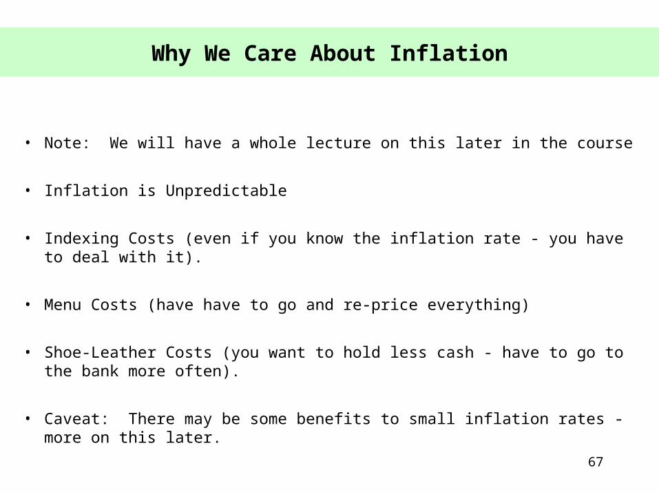
Why We Care About Inflation
• Note: We will have a whole lecture on this later in the course
• Inflation is Unpredictable
• Indexing Costs (even if you know the inflation rate - you have to deal with it).
• Menu Costs (have have to go and re-price everything)
• Shoe-Leather Costs (you want to hold less cash - have to go to the bank more often).
• Caveat: There may be some benefits to small inflation rates - more on this later.

68
Why We Care About Inflation
• An Example of how inflation can affect real returns.
• Suppose we agree that a real rate of 0.05 over the next year is fair. – borrowing rate, salary growth rate, etc.
• Suppose we also agree that expected inflation over the next year is 0.07.
• We should then set the nominal return equal to 0.12 (i = re + лe)
Summary: i = 0.12
re = 0.05
лe = 0.07

69
Why We Care About Inflation
• Suppose that actual inflation is 0.10 (лa > лe)
In this case, ra = 0.02 (ra = i - лa)
Borrowers/Firms are better off
Lenders/Workers worse off
• Suppose that actual inflation is 0.03 (лa < лe)
In this case, ra = 0.09 (ra = i - лa)
Borrowers/Firms are worse off
Lenders/Workers better off
It has been shown that higher inflation rates are correlated with more variability. People/Firms Don’t Like the Uncertainty
70
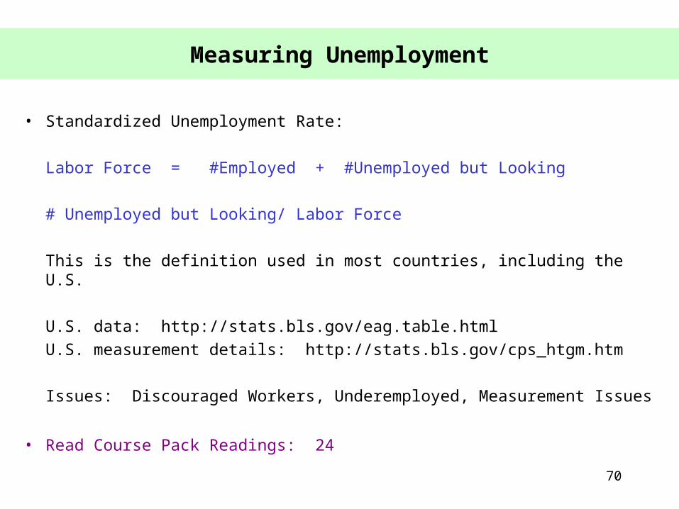
Measuring Unemployment
• Standardized Unemployment Rate:
Labor Force = #Employed + #Unemployed but Looking
# Unemployed but Looking/ Labor Force
This is the definition used in most countries, including the U.S.
U.S. data: http://stats.bls.gov/eag.table.html
U.S. measurement details: http://stats.bls.gov/cps_htgm.htm
Issues: Discouraged Workers, Underemployed, Measurement Issues
• Read Course Pack Readings: 24

71
Types of Unemployment
• Frictional Unemployment: Result of Matching Behavior between Firms and Workers.
• Structural Unemployment: Result of Mismatch of Skills and Employer Needs
• Cyclical Unemployment: Result of Output being below full-employment
• Is Zero Unemployment a Reasonable Policy Goal?– No! Frictional and Structural Unemployment may be desirable (unavoidable).

72
Why We Care About Unemployment
• Depreciation of Human Capital
• Productive Externalities
• Social Externalities
• Individual Self Worth

73
Understanding Housing Prices
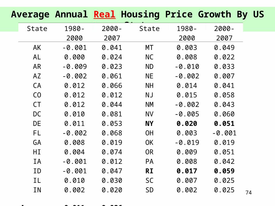
Average Annual Real Housing Price Growth By US State
State 1980-2000 2000-2007 State 1980-2000 2000-2007AK -0.001 0.041 MT 0.003 0.049AL 0.000 0.024 NC 0.008 0.022AR -0.009 0.023 ND -0.010 0.033AZ -0.002 0.061 NE -0.002 0.007CA 0.012 0.066 NH 0.014 0.041CO 0.012 0.012 NJ 0.015 0.058CT 0.012 0.044 NM -0.002 0.043DC 0.010 0.081 NV -0.005 0.060DE 0.011 0.053 NY 0.020 0.051FL -0.002 0.068 OH 0.003 -0.001GA 0.008 0.019 OK -0.019 0.019HI 0.004 0.074 OR 0.009 0.051IA -0.001 0.012 PA 0.008 0.042ID -0.001 0.047 RI 0.017 0.059IL 0.010 0.030 SC 0.007 0.025IN 0.002 0.020 SD 0.002 0.025
Average 0.011 0.03674
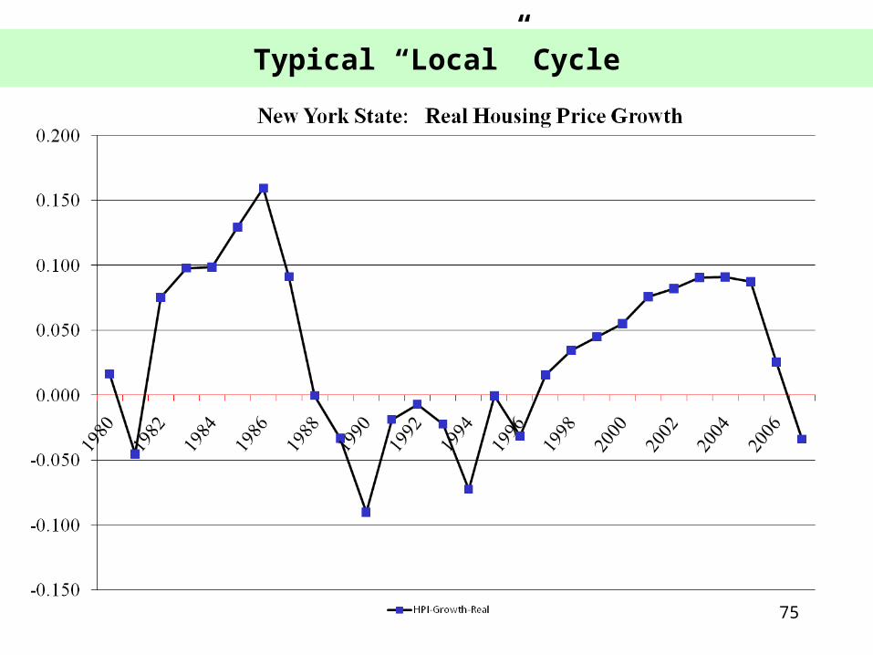
Typical “Local” Cycle
75
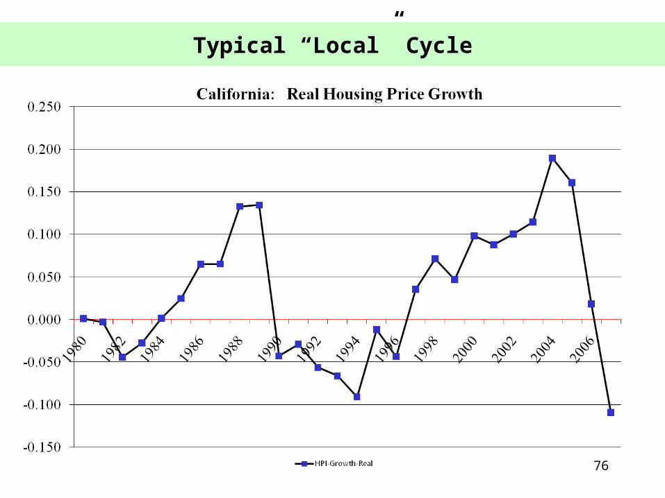
Typical “Local” Cycle
76
77

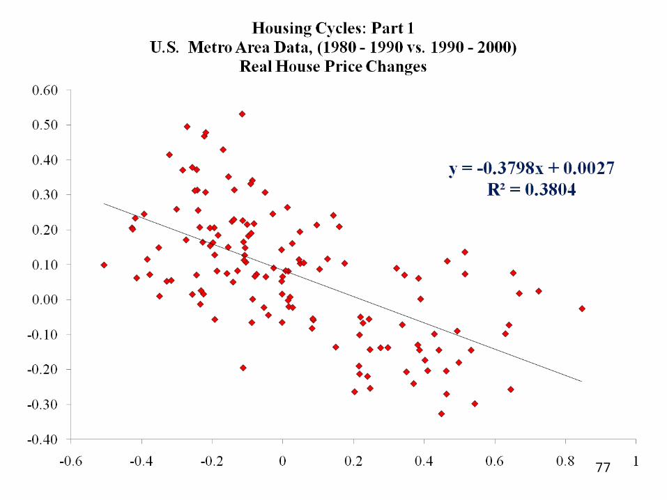
Housing Prices and Housing Cycles (Hurst and Guerrieri (2009))
• Persistent housing price increases are ALWAYS followed by persistent housing price declines
Some statistics about U.S. metropolitan areas 1980 – 2000
• 44 MSAs had price appreciations of at least 15% over 3 years during this period.
• Average price increase over boom (consecutive periods of price increases): 55%
• Average price decline during bust (the following period of price declines): 30%
• Average length of bust: 26 quarters (i.e., 7 years)
• 40% of the price decline occurred in first 2 years of bust 78

79
AKAL
AR
AZ
CA
CO
CT
DCDE
FL
GAHI
IAID
ILIN
KSKY
LA
MAMD
ME
MI
MN
MOMS
MTNC
ND
NE
NHNJ
NM
NV
NY
OH
OK
ORPA
RI
SCSD
TN
TXUT
VA
VTWA
WI
WV
-.8
-.6
-.4
-.2
0
0 .5 1g_97_05
g_05_09 Fitted values
Real House Price Changes By State: 1997-2005 (x-axis) vs. 2005 – 2009 (y-axis)

Typical “Country” Cycle (US – OFHEO Data)
U.S. Nominal House Price Appreciation: 1976 - 2008
80

Typical “Country” Cycle (US – OFHEO Data)
U.S. Real House Price Appreciation: 1976 - 2008
81

Country 1970-1999 2000-2006 Country 1970-1999 2000-2006
U.S. 0.012 0.055 Netherlands 0.023 0.027Japan 0.010 -0.045 Belgium 0.019 0.064
Germany 0.001 -0.029 Sweden -0.002 0.059France 0.010 0.075 Switzerland 0.000 0.019
Great Britain 0.022 0.068 Denmark 0.011 0.065Italy 0.012 0.051 Norway 0.012 0.047
Canada 0.013 0.060 Finland 0.009 0.040Spain 0.019 0.081 New Zealand 0.014 0.080
Australia 0.015 0.065 Ireland 0.022 0.059
Average 1970-1999 0.0122000-2006 0.046
Average Annual Real Price Growth By OECD Country
82

Country Cycles – The U.S. is Not Alone
83
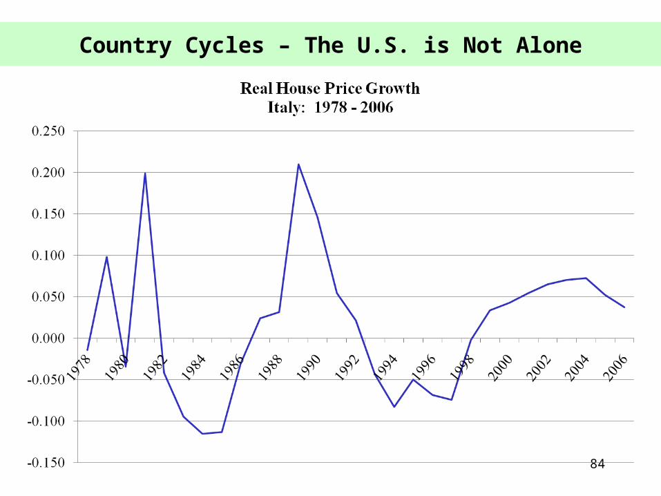
Country Cycles – The U.S. is Not Alone
84

Country Cycles – The U.S. is Not Alone
85

86
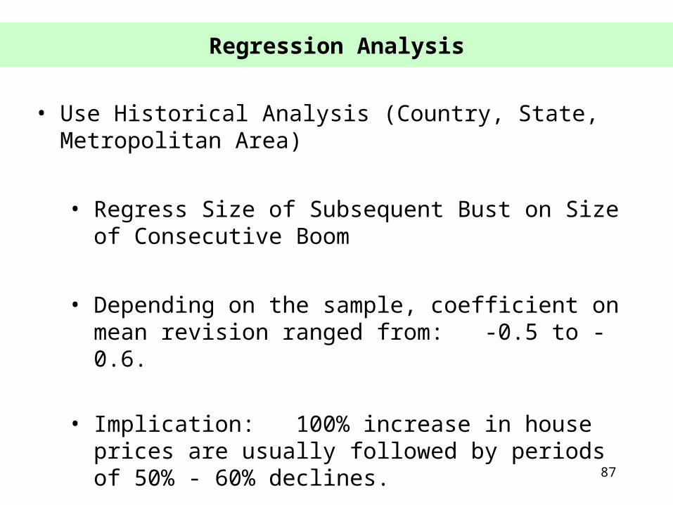
Regression Analysis
• Use Historical Analysis (Country, State, Metropolitan Area)
• Regress Size of Subsequent Bust on Size of Consecutive Boom
• Depending on the sample, coefficient on mean revision ranged from: -0.5 to -0.6.
• Implication: 100% increase in house prices are usually followed by periods of 50% - 60% declines.
87

88
Equilibrium in Housing Markets
Demand
PH
QH
Fixed Supply (Short Run)

89
Equilibrium in Housing Markets
Demand
PH
QH
Fixed Supply (Short Run)
PH’

90
Equilibrium in Housing Markets
Demand
PH
QH
Fixed Supply (Short Run)
PH’
Demand shocks cause large price increases when supply is fixed

91
Equilibrium in Housing Markets
Demand
PH
QH
Fixed Supply
PH’Supply Eventually Adjusts
PH”

How Does Supply Adjust?
• Build on Vacant Land
• Convert Rental or Commercial Property
• Build Up
• Build Out (Suburbs)
• Build Way Out (Create New Cities)
• Some of these adjustments can take consider amounts of time.
92

Do Supply Factors Explain 2000-2008 Cycle
Change in Total Housing Units Against Change in Housing Price
Adjusted for Population Changes (2000-2005, State Level)
93
AK
AL
AR
AZ CA
CO
CTDC
DEFL
GA
HI
IA
ID
IL
IN
KSKY
LA
MA
MD
ME
MI
MN
MO
MS
MT
NC
ND
NE
NHNJ
NM
NV
NY
OH
OK
OR
PA
RI
SC SD
TN
TX
UT
VA
VTWA
WI
WVWY
-.04
-.02
0.0
2.0
4
-.2 0 .2 .4 .6Residuals
Residuals Fitted values

Do Supply Factors Explain 2000-2008 Cycle
Change in Total Housing Units Against Change in Housing Price
Adjusted for Population Changes (2005-2009, State Level)
94
AK
AL
AR
AZ
CACO
CT
DC
DE
FL
GA
HI
IA
ID
IL
INKS
KY
LA
MA
MD
MEMI
MN
MO
MS
MT
NC
ND
NE
NH
NJ
NM
NV
NY
OH
OKORPA
RISC
SDTN
TX
UT
VA VTWA
WIWV
WY
-.03
-.02
-.01
0.0
1.0
2
-.6 -.4 -.2 0 .2Residuals
Residuals Fitted values

Country 1970-1999 2000-2006 Country 1970-1999 2000-2006
U.S. 0.012 0.055 Netherlands 0.023 0.027Japan 0.010 -0.045 Belgium 0.019 0.064
Germany 0.001 -0.029 Sweden -0.002 0.059France 0.010 0.075 Switzerland 0.000 0.019
Great Britain 0.022 0.068 Denmark 0.011 0.065Italy 0.012 0.051 Norway 0.012 0.047
Canada 0.013 0.060 Finland 0.009 0.040Spain 0.019 0.081 New Zealand 0.014 0.080
Australia 0.015 0.065 Ireland 0.022 0.059
Average 1970-1999 0.0122000-2006 0.046
Average Annual Real Price Growth By OECD Country
95

What Does This All Mean
• Decline in Residential Housing Prices in the U.S. was very predictable (although the timing was not).
• Using OFHEO price index, real housing prices rose by 46% between 1997 and 2006 (for the entire U.S.).
• My model predicts that housing prices will fall by roughly 25-30% (in real terms) over the next 5-7 years.
• So far, the real OFHEO price index has fallen by roughly 15-20% (from peak to current levels).
• More “real” residential price declines to come! (Nominal prices should stabilize late this year/early next year).
96

U.S. OFHEO Housing Cycle - Levels
97

98
Bonus Material: The Yield Curve

99
What is a Yield Curve
• A yield curve graphs the interest rate for a given security of differing maturities.• For example, it represents the yield on 1, 3, 5, 7, and 10 year treasuries.
Historically, yield curves tend to be upward slopingData on U.S. treasury yields from late 2004
Maturity (in years)

100
Yield Curve Mechanics
• Consider a two period model
• Define the interest rate on a one year treasury starting today as i0,1
• Define the interest rate on a two year treasury starting today as i0,2
• What is the relationship between one year treasuries and two year treasuries?
• Appeal to theory of arbitrage. If arbitrage holds, then by definition:
(1 + i0,2)2 = (1 + i0,1) * (1 + i1,2)
where i1,2 is the interest rate on a one year treasury starting one period from now.

101
Shape of the Yield Curve: Macro Explanations
• Solve for long interest rates (i0,2) as a function of short rates:
i0,2 = [(1+i0,1) * (1+i1,2)]1/2 – 1
• Question: When does the yield curve slope up (i.e., i0,2 > i0,1)?
• Answer: When i1,2 > i0,1

102
Shape of the Yield Curve: Macro Explanations
• When does i1,2 > i0,1 ?
• Remember: i = r + πe + ρ (or, with time subscripts, i0,1 = r0,1 + πe0,1 + ρ0,1)
where ρ is a risk premium
• To start, assume risk free assets (ρ = 0)
• So, if r is held fixed over time (i.e., r0,1 = r1,2) then the yield curve will slope up if πe
1,2 > πe0,1. Increasing inflation will cause the yield curve to slope up (all else
equal)!
• Also, if πe is fixed over time (i.e., πe
1,2 = πe0,1) then the yield curve will slope up if
r1,2 > r0,1. Higher future real rates will cause the yield curve to slope up (all else equal).

103
Shape of the Yield Curve: Micro Explanations
• Suppose ρ is not equal to zero such that:
i = r + π + ρ
• Alluding back to our previous discussion, i1,2 > i0,1 if ρ1,2 > ρ0,1
• Components of ρ include default premiums and term premiums
• Changes in ρ for long term assets relative to short term assets (i.e., a decline in the term premium) will affect shape of the yield curve.
• See an interesting discussion by Ben Bernanke on the shape of yield curves:http://www.federalreserve.gov/boarddocs/Speeches/2006/20060320/default.htm

104
Flat or Inverted Yield Curves
• There is no reason that yield curves need to slope upwards. Expected future short term rates could be the same or lower than current short term rates. This would imply that current long rates will be the same or lower than current short rates.
• This will lead to flat yield curves (current short rates = current long rates) or inverted yield curves (current short rates > current long rates).
• This possibility could exist in equilibrium! This will occur if inflation is expected to decline over time (or if deflation is predicted), if future expectations of real interest rates are lower than current real interest rates, and if risk premiums in the future are thought to decline.
• Key: Some people assume that a flat or inverted yield curve means that the economy will be entering a recession! This is not always true. But, demand side recessions cause both r and expected inflation to fall.

105
Current Yield Curve for U.S. Treasuries (12/1/09)
0
0.5
1
1.5
2
2.5
3
3.5

106
Other Flattening of the Yield Curve: Micro Explanations
• One component of the term premium: Uncertainty in the future
– If investors are risk averse and the government is risk neutral, an equilibrium could exist where the government will compensate borrowers for holding longer term assets.
– A decline in uncertainty (perhaps due to the “Great Moderation”) could flatten yield curves relative to historical standards.
• A second component of the term premium: Liquidity premium
– If short term assets are more liquid than long term assets (or demand for short term assets is relatively higher than long term assets), a risk premium will exist.
– An increase in the demand for long term U.S. assets (perhaps by foreign investors) could cause the yield curve to flatten.

107
Current “10”- “2” Year Treasury (Through 2/09)