winter 2014parallel processing, circuit-level parallelismslide 1 part ii circuit-level parallelism...

Winter 2014 Parallel Processing, Circuit-Level Parallelism Slide 1

Part IICircuit-Level Parallelism

Part IICircuit-Level Parallelism

7. Sorting and Selection Networks8A. Search Acceleration Circuits6B. Arithmetic and Counting Circuits6C. Fourier Transform Circuits

Sorting and Searching

Numerical Computations


About This Presentation

This presentation is intended to support the use of the textbook Introduction to Parallel Processing: Algorithms and Architectures (Plenum Press, 1999, ISBN 0-306-45970-1). It was prepared by the author in connection with teaching the graduate-level course ECE 254B: Advanced Computer Architecture: Parallel Processing, at the University of California, Santa Barbara. Instructors can use these slides in classroom teaching and for other educational purposes. Any other use is strictly prohibited. © Behrooz Parhami

Edition Released Revised Revised Revised

First Spring 2005 Spring 2006 Fall 2008 Fall 2010

Winter 2013 Winter 2014


II Circuit-Level Parallelism

Circuit-level specs: most realistic parallel computation model• Concrete circuit model; incorporates hardware details• Allows realistic speed and cost comparisons• Useful for stand-alone systems or acceleration units

Topics in This Part

Chapter 7 Sorting and Selection Networks

Chapter 8A Search Acceleration Circuits

Chapter 8B Arithmetic and Counting Circuits

Chapter 8C Fourier Transform Circuits


7 Sorting and Selection Networks Become familiar with the circuit model of parallel processing:

• Go from algorithm to architecture, not vice versa• Use a familiar problem to study various trade-offs

Topics in This Chapter

7.1 What is a Sorting Network?

7.2 Figures of Merit for Sorting Networks

7.3 Design of Sorting Networks

7.4 Batcher Sorting Networks

7.5 Other Classes of Sorting Networks

7.6 Selection Networks


7.1 What is a Sorting Network?

Fig. 7.1 An n-input sorting network or an n-sorter.

xxx

x

.

.

.

.

.

.

n-sorter

0

1

2

n–1

yyy

y

0

1

2

n–1

The outputs are a permutation of the inputs satisfying y Š y Š ... Š y (non-descending)

0 1 n–1

Fig. 7.2 Block diagram and four different schematic representations for a 2-sorter.

2-sorter

input min0

input1 max

in out

in out

Block Diagram Alternate Representations

in out

in out


2-sorter

input min0

input1 max

in out

in out

Block Diagram Alternate Representations

in out

in out

2-sorter

Building Blocks for Sorting Networks

Fig. 7.3 Parallel and bit-serial hardware realizations of a 2-sorter.

Q R

S

Com-pare

1

0

1

0

k

k

k

k

min(a, b )

max(a, b )

b<a?

a

b

Q R

S

1

0

1

0

min(a, b )

max(a, b )

b<a?

a

b M

SB

-firs

t ser

ial i

nput

s

a<b?

Reset

Implementation with bit-parallel inputs

Implementation with bit-serial inputs


Proving a Sorting Network Correctx0x1

x

x3

2

y0

y1

y

y3

2

2

3

1

5

3

2

5

1

1

3

2

5

1

2

3

5

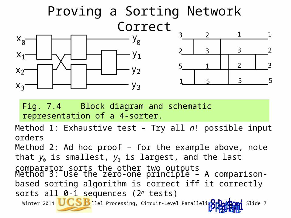
Fig. 7.4 Block diagram and schematic representation of a 4-sorter.

Method 1: Exhaustive test – Try all n! possible input orders

Method 2: Ad hoc proof – for the example above, note that y0 is smallest, y3 is largest, and the last comparator sorts the other two outputs

Method 3: Use the zero-one principle – A comparison-based sorting algorithm is correct iff it correctly sorts all 0-1 sequences (2n tests)


Elaboration on the Zero-One Principle

Deriving a 0-1 sequence that is not correctly sorted, given an arbitrary sequence that is not correctly sorted.

Let outputs yi and yi+1 be out of order, that is yi > yi+1

Replace inputs that are strictly less than yi with 0s and all others with 1s

The resulting 0-1 sequence will not be correctly sorted either

6-sorter

1 3 6* 5* 8 9

3 6 9 1 8 5

Invalid

0 1 1 0 1 0

0 0 1 0 1 1


7.2 Figures of Merit for Sorting Networks

Delay: Number of levels

Cost: Number of comparators

Cost Delay

x0x1

x

x3

2

y0

y1

y

y3

2

2

3

1

5

3

2

5

1

1

3

2

5

1

2

3

5

In the following example, we have 5 comparators

The following 4-sorter has 3 comparator levels on its critical path

The cost-delay product for this example is 15

Fig. 7.4 Block diagram and schematic representation of a 4-sorter.


Cost as a Figure of Merit

n = 9, 25 modules, 9 levelsn = 10, 29 modules, 9 levels

n = 12, 39 modules, 9 levels

n = 16, 60 modules, 10 levelsFig. 7.5 Some low-cost sorting networks.

Optimal size is known for n = 1 to 8: 0, 1, 3, 5, 9, 12, 16, 19




Delay as a Figure of Merit

Fig. 7.6 Some fast sorting networks.





Optimal delay is known for n = 1 to 10: 0, 1, 3, 3, 5, 5, 6, 6, 7, 7

These 3 comparators constitute one level


Cost-Delay Product as a Figure of Merit





Fast 10-sorter from Fig. 7.6




Low-cost 10-sorter from Fig. 7.5

Cost Delay = 29 9 = 261

Cost Delay = 31 7 = 217

The most cost-effective n-sorter may be neither the fastest design, nor the lowest-cost design


7.3 Design of Sorting Networks

Fig. 7.7 Brick-wall 6-sorter based on odd–even transposition.

Rotate by 90 degrees

Rotate by 90 degrees to see the odd-even exchange patterns

C(n) = n(n – 1)/2D(n ) = n

Cost Delay = n2(n – 1)/2 = (n3)


Insertion Sort and Selection Sort

Fig. 7.8 Sorting network based on insertion sort or selection sort.

xxx

x

.

.

.

(n–1)-sorter

0

1

2

n–2

yyy

y

0

1

2

n–2

x n–1

.

.

.

y n–1

xxx

x

.

.

.

(n–1)-sorter

0

1

2

n–2

yyy

y

0

1

2

n–2

x n–1

.

.

.

y n–1

.

.

.

Insert ion sort Selection sort

Parallel insertion sort = Parallel selection sort = Parallel bubble sort!

C(n) = n(n – 1)/2D(n ) = 2n – 3 Cost Delay = (n3)


Theoretically Optimal Sorting Networks

AKS sorting network(Ajtai, Komlos, Szemeredi: 1983)

xxx

x

.

.

.

.

.

.

n-sorter

0

1

2

n–1

yyy

y

0

1

2

n–1

The outputs are a permutation of the inputs satisfying y Š y Š ... Š y (non-descending)

0 1 n–1

O(log n) depth

O(n log n)size

Unfortunately, AKS networks are not practical owing to large (4-digit) constant factors involved; improvements since 1983 not enough

Note that even for these optimal networks, delay-cost product is suboptimal; but this is the best we can do

Existing sorting networks have O(log2 n) latency and O(n log2 n) cost

Given that log2 n is only 20 for n = 1 000 000, the latter are more practical


7.4 Batcher Sorting Networks

Fig. 7.9 Batcher’s even–odd merging network for 4 + 7 inputs.

x

x

x

x

y

y

y

y

y

y

y v

v

v

v

v

v

0

1

2

3

0

1

2

3

4

5

6

0

1

2

3

4

5

w

w

w

w

w

0

1

2

3

4

(2, 4)-merger (2, 3)-merger

First sorted sequence x

Second sorted sequence y

(2, 3)-mergera0a1

b0b1b2

(1, 2)-mergerc0

d0d1

(1, 1) (1, 2)

(1, 1)


Proof of Batcher’s Even-Odd Mergex

x

x

x

y

y

y

y

y

y

y v

v

v

v

v

v

0

1

2

3

0

1

2

3

4

5

6

0

1

2

3

4

5

w

w

w

w

w

0

1

2

3

4

(2, 4)-merger (2, 3)-merger

First sorted sequence x

Second sorted sequence y

Use the zero-one principle

Assume: x has k 0sy has k 0s

Case a: keven = kodd v 0 0 0 0 0 0 1 1 1 1 1 1 w 0 0 0 0 0 0 1 1 1 1 1

Case b: keven = kodd+1 v 0 0 0 0 0 0 0 1 1 1 1 1 w 0 0 0 0 0 0 1 1 1 1 1

Case c: keven = kodd+2 v 0 0 0 0 0 0 0 0 1 1 1 1 w 0 0 0 0 0 0 1 1 1 1 1

Out of order

v has keven = k/2 + k /2 0s

w has kodd = k/2 + k /2 0s


Batcher’s Even-Odd Merge SortingBatcher’s (m, m) even-odd merger, for m a power of 2:

C(m) = 2C(m/2) + m – 1 = (m – 1) + 2(m/2 – 1) + 4(m/4 – 1) + . . . = m log2m + 1

D(m) = D(m/2) + 1 = log2 m + 1

Cost Delay = (m log2 m)Batcher sorting networks based on the even-odd merge technique:

C(n) = 2C(n/2) + (n/2)(log2(n/2)) + 1 n(log2n)2/ 2

D(n) = D(n/2) + log2(n/2) + 1 = D(n/2) + log2n = log2n (log2n + 1)/2

Cost Delay = (n log4n)

n/2-sorter

n/2-sorter

(n/2, n/2)- merger

.

.

.

.

.

.

.

.

.

.

.

.

.

.

.

.

.

.

Fig. 7.10 The recursive structure of Batcher’s even–odd merge sorting network.


Example Batcher’s Even-Odd 8-Sorter

n/2-sorter

n/2-sorter

(n/2, n/2)- merger

.

.

.

.

.

.

.

.

.

.

.

.

.

.

.

.

.

.

4-sorters Even (2,2)-merger

Odd (2,2)-merger

Fig. 7.11 Batcher’s even-odd merge sorting network for eight inputs .


Bitonic-Sequence Sorter

Fig. 14.2 Sorting a bitonic sequence on a linear array.

Shift right half of data to left half (superimpose the two halves)

In each position, keep the smaller value of each pair and ship the larger value to the right

Each half is a bitonic sequence that can be sorted independently

0 1 2 n–1

0 1 2 n–1

. . .

. . .

Bitonic sequence

Shifted right half

n/2

n/2

. . .

. . .

Bitonic sequence:

1 3 3 4 6 6 6 2 2 1 0 0 Rises, then falls

8 7 7 6 6 6 5 4 6 8 8 9 Falls, then rises

8 9 8 7 7 6 6 6 5 4 6 8 The previous sequence, right-rotated by 2


Batcher’s Bitonic Sorting Networks

Fig. 7.12 The recursive structure of Batcher’s bitonic sorting network.

n/2-sorter

n/2-sorter

n-input bitonic- sequence sorter

.

.

.

.

.

.

.

.

.

.

.

.

.

.

.

.

.

.

Bitonic sequence

. . .

. . .

Fig. 7.13 Batcher’s bitonic sorting network for eight inputs.

8-input bitonic- sequence sorter

4-input bitonic- sequence sorters

2-input sorters


7.5 Other Classes of Sorting Networks

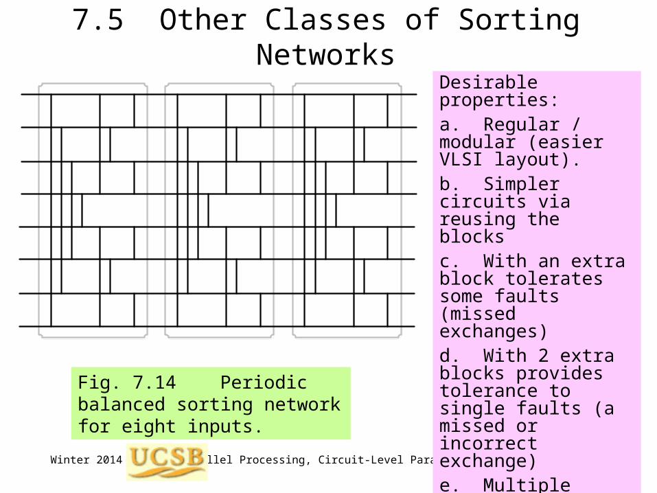
Fig. 7.14 Periodic balanced sorting network for eight inputs.

Desirable properties:a. Regular / modular (easier VLSI layout).b. Simpler circuits via reusing the blocksc. With an extra block tolerates some faults (missed exchanges)d. With 2 extra blocks provides tolerance to single faults (a missed or incorrect exchange)e. Multiple passes through faulty network (graceful degradation)f. Single-block design becomes fault-tolerant by using an extra stage


Shearsort-Based Sorting Networks (1)

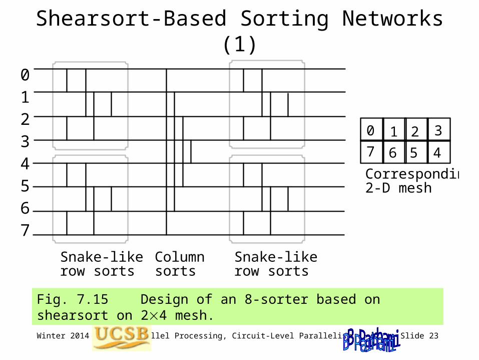
Fig. 7.15 Design of an 8-sorter based on shearsort on 24 mesh.

0 1 2 3

4567

Snake-like row sorts

Column sorts

0 1 2 3 4 5 6 7

Snake-like row sorts

Corresponding 2-D mesh


Shearsort-Based Sorting Networks (2)

Fig. 7.16 Design of an 8-sorter based on shearsort on 24 mesh.

0 1 2 3 4 5 6 7

0 1

3 2

54

7 6

Corresponding 2-D mesh

Left column sort

Right column sort

Snake-like row sort

Left column sort

Right column sort

Snake-like row sort

Some of the sameadvantages asperiodic balancedsorting networks


7.6 Selection NetworksDirect design may yield simpler/faster selection networks

4-sorters Even (2,2)-merger

Odd (2,2)-merger

3rd smallest element

Can remove this block if smallest three inputs needed

Can remove these four comparators

Deriving an (8, 3)-selector from Batcher’s even-odd merge 8-sorter.


Categories of Selection Networks

Unfortunately we know even less about selection networks than we do about sorting networks.

One can define three selection problems [Knut81]:

I. Select the k smallest values; present in sorted order II. Select kth smallest value III. Select the k smallest values; present in any order

Circuit and time complexity: (I) hardest, (III) easiest

Type-I

8 inputs (8, 4)-selector

Smallest2nd smallest3rd smallest4th smallest

4th smallest

Type-IIThe 4 smallestIn any order

Type-III


Type-III Selection Networks

[0,7]

[0,7]

[0,7]

[0,7]

[0,7]

[0,7]

[0,7]

[0,7]

[0,6]

[1,7]

[0,6]

[0,6]

[0,6]

[1,7]

[1,7]

[1,7]

[1,6]

[1,6]

[1,6]

[1,6]

[0,3]

[0,4]

[0,4]

[0,4]

[0,4] [0,3]

[3,7]

[4,7][3,7][3,7]

[3,7]

[4,7]

[1,3]

[1,5]

[1,5] [1,3]

[4,6][2,6]

[2,6]

[4,6]

Figure 7.17 A type III (8, 4)-selector. 8-Classifier


Classifier Networks

Use of classifiers for building sorting networks

Classifiers:Selectors that separate the smaller half of values from the larger half

Smaller4 values

Larger4 values

8 inputs 8-Classifier

8-Classifier

4-Classifier

4-Classifier

2-Classifier

2-Classifier

2-Classifier

2-Classifier

Problem: Given O(log n)-time and O(n log n)-cost n-classifier designs, what are the delay and cost of the resulting sorting network?


8A Search Acceleration Circuits Much of sorting is done to facilitate/accelerate searching

• Simple search can be speeded up via special circuits• More complicated searches: range, approximate-match


8A.1 Systolic Priority Queues

8A.2 Searching and Dictionary Operations

8A.3 Tree-Structured Dictionary Machines

8A.4 Associative Memories

8A.5 Associative Processors

8A.6 VLSI Trade-offs in Search Processors


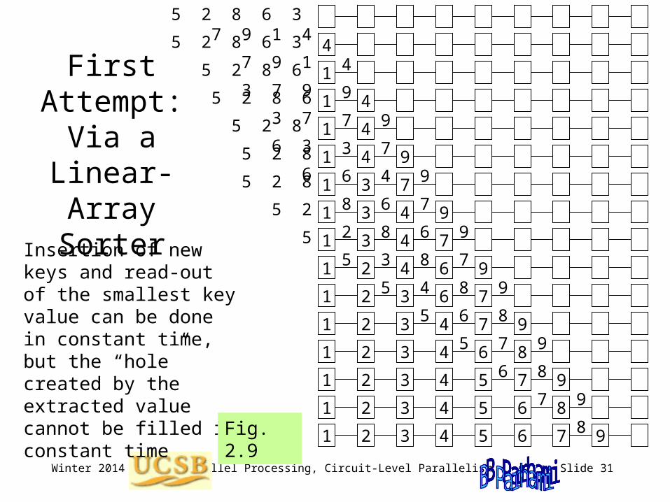
8A.1 Systolic Priority Queues

Problem: We want to maintain a large list of keys, so that we can add new keys into it (insert operation) and obtain the smallest key (extract operation) whenever desired.

Unsorted list: Constant-time insertion / Linear-time extraction

Sorted list: Linear-time insertion / Constant-time extraction

Can both insert and extract operations (priority-queue operations) be performed in constant time, independent of the size of the list?

Priority queue

3 7 9 1 45 2 8 6 1


5 2 8 6 3 7 9 1 4

5 2 8 6 3 7 9 1 4

1

1 4

5 2 8 6 3 7 9

1 4

4

1 4 9

95 2 8 6 3 7

1 3 7

9

1 3 4 9

75 2 8 6 3

1 3 4 78

1 2 4 6 9

9

1 2 3 6 7

1 2 3 4 7 9

1 2 3 4 6 8

1 2 3 4 5 7 9

1 2 3 4 5 6 8

1 2 3 4 5 6 7 9

9

5 2 8 6

First Attempt: Via a Linear-Array Sorter

Insertion of new keys and read-out of the smallest key value can be done in constant time, but the “hole” created by the extracted value cannot be filled in constant time

3 7

8 6

6 45 2 875 2

5 2 6

3 8 75

4 8 95

6 85

7 95

8

7 9

6

8Fig. 2.9


Operating on every other clock cycle, allows holes to be filled

A Viable Systolic Priority Queue

5 -- 2 -- 8 -- 6 -- 3 -- 7 -- 9 -- 1 -- 4

5 -- 2 -- 8 -- 6 -- 3 -- 7 -- 9 -- 1 --

5 -- 2 -- 8 -- 6 -- 3 -- 7 -- 9 -- 1

4

4

5 -- 2 -- 8 -- 6 -- 3 -- 7 -- 9 -- 1

5 -- 2 -- 8 -- 6 -- 3 -- 7 -- 9 1 4

4

5 -- 2 -- 8 -- 6 -- 3 -- 7 -- 1 49

5 -- 2 -- 8 -- 6 -- 3 -- 7 1 4 9

5 -- 2 -- 8 -- 6 -- 3 -- 1 4 97

5 -- 2 -- 8 -- 6 -- 3 1 4 97

Extract 1 4 7 9

4 7 9

Extract 4 7 9

7 9

Extract 7 9

9 5 -- 2 -- 8 -- 6 -- 3

3 95 -- 2 -- 8 -- 6 --


S LM

S LM

S LM

S LM

S LM

S LM

S LM

S LM

S LM

S LM

S LM

S LM

S LM

S LM

S LM

Systolic Data Structures

Fig. 8.3 Systolic data structure for minimum, maximum,

and median finding.

Each node holds the smallest (S), median (M),and largest (L)value in its subtree

Each subtree is balanced or has one fewer element on the

left (root flag shows this)

[5, 87] [87, 176]Insert 2 Insert 20 Insert 127 Insert 195

Extractmin Extractmed Extractmax19 or 20

items 20 items

176587

Update/access examples for the systolic data structure of Fig. 8.3

Example: 20 elements,3 in root, 8 on left,

and 9 on right

8 elements:3 + 2 + 3


8A.2 Searching and Dictionary Operations

Example:n = 26, p = 2

P0

P1

0 1 2

25

8

17

P0

P1P0P1

Example: n = 26 p = 2

Step 2

Step 1

Step 0

A single search in a sorted list can’t be significantly speeded up through parallel processing, but all hope is not lost:

Dynamic data (sorting overhead)

Batch searching (multiple lookups)

Parallel (p + 1)-ary search on PRAM

logp+1(n + 1) = log2(n + 1) / log2(p + 1) = (log n / log p) steps

Speedup log p

Optimal: no comparison-based search algorithm can be faster


Dictionary OperationsBasic dictionary operations: record keys x0, x1, . . . , xn–1

search(y) Find record with key y; return its associated datainsert(y, z) Augment list with a record: key = y, data = zdelete(y) Remove record with key y; return its associated data

Some or all of the following operations might also be of interest:

findmin Find record with smallest key; return datafindmax Find record with largest key; return datafindmed Find record with median key; return datafindbest(y) Find record with key “nearest” to yfindnext(y) Find record whose key is right after y in sorted orderfindprev(y) Find record whose key is right before y in sorted orderextractmin Remove record(s) with min key; return dataextractmax Remove record(s) with max key; return dataextractmed Remove record(s) with median key value; return data

Priority queue operations: findmin, extractmin (or findmax, extractmax)


8A.3 Tree-Structured Dictionary Machines

Fig. 8.1 A tree-structured dictionary machine.

x

Input Root

Output Root

"Circle" Tree

"Triangle" Tree

0 x1 x2 x4x3 x5 x6 x7

Combining in the triangular nodes

search(y): Pass OR of match signals & data from “yes” side

findmin / findmax: Pass smaller / larger of two keys & data

findmed:Not supported here

findbest(y): Pass the larger of two match-degree indicators along with associated record

Search 1

Search 2 Pipelinedsearch


Insertion and Deletion in the Tree Machine

Figure 8.2 Tree machine storing 5 records and containing 3 free slots.

*

Input Root

Output Root

* ** *

insert(y,z)

0 1

0 0 1 0 0 0 1 1

0 2

1 20

Counters keep track of the vacancies in each subtree

Deletion needs second pass to update the vacancy counters

Redundant insertion (update?) and deletion (no-op?)

Implementation:Merge the circle and

triangle trees by folding


Physical Realization of a Tree Machine

Tree machine in folded form

Leaf node

Inner node


VLSI Layout of a Tree

H-tree layout (used, e.g., for clock distribution network in high-performance microchips)

A clockdomain


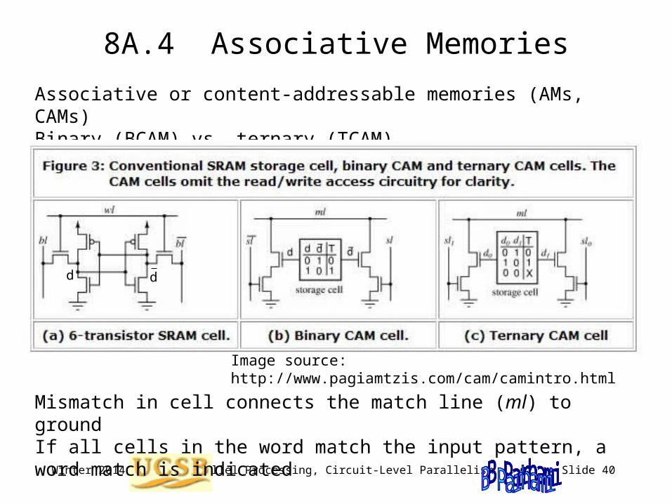
8A.4 Associative Memories

Associative or content-addressable memories (AMs, CAMs) Binary (BCAM) vs. ternary (TCAM)

Image source: http://www.pagiamtzis.com/cam/camintro.html

Mismatch in cell connects the match line (ml) to groundIf all cells in the word match the input pattern, a word match is indicated

d d


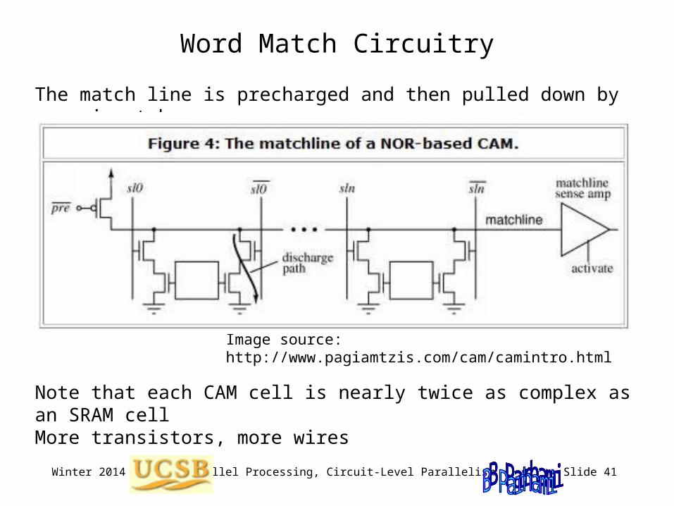
Word Match Circuitry

The match line is precharged and then pulled down by any mismatch


Note that each CAM cell is nearly twice as complex as an SRAM cellMore transistors, more wires


CAM Array Operation



Current CAM Applications

Packet forwardingRouting tables specify the path to be taken by matching an incoming destination address with stored address prefixesPrefixes must be stored in order of decreasing length (difficult updating)

Packet classificationDetermine packet category based on information in multiple fieldsDifferent classes of packets may be treated differently

Associative caches / TLBsMain processor caches are usually not fully associative (too large)Smaller specialized caches and TLBs benefit from full associativity

Data compressionFrequently used substrings are identified and replaced by short codesSubstring matching is accelerated by CAM


History of Associative Processing

Table 4.1 Entering the second half-century of associative processing ––––––––––––––––––––––––––––––––––––––––––––––––––––––––––––––––––––– Decade Events and Advances Technology Performance––––––––––––––––––––––––––––––––––––––––––––––––––––––––––––––––––––– 1940s Formulation of need & concept Relays 1950s Emergence of cell technologies Magnetic, Cryogenic Mega-bit-OPS 1960s Introduction of basic architectures Transistors 1970s Commercialization & applications ICs Giga-bit-OPS 1980s Focus on system/software issues VLSI Tera-bit-OPS 1990s Scalable & flexible architectures ULSI, WSI Peta-bit-OPS–––––––––––––––––––––––––––––––––––––––––––––––––––––––––––––––––––––

Associative memory Parallel masked search of all words Bit-serial implementation with RAM

Associative processor Add more processing logic to PEs

100111010110001101000 ComparandMask

Memory array with comparison logic


8A.5 Associative Processors

Fig. 23.1 Functional view of an associative memory/processor.

.

.

.

Global Operations Control & Response

Cell 0

Cell 1

Cell 2

Cell m–1

Data and Commands Broadcast

Read Lines Response

Store (Tags)

Global Tag Operations Unit

Control Unit

Comparand

Mask

tm–1

t2

t1

t 0

.

.

.

.

.

.

Associative or content-addressable memories/processors constituted early forms of SIMD parallel processing


Search Functions in Associative Devices

Exact match: Locating data based on partial knowledge of contents

Inexact match: Finding numerically or logically proximate values

Membership: Identifying all members of a specified set

Relational: Determining values that are less than, less than or equal, etc.

Interval: Marking items that are between or outside given limits

Extrema: Finding the maximum, minimum, next higher, or next lower

Rank-based: Selecting kth or k largest/smallest elements

Ordered retrieval: Repeated max- or min-finding with elimination (sorting)


Classification of Associative Devices

WPBP:Fully

parallel

WPBS:Bit-

serial

WSBS:Fully serial

WSBP:Word-serial

Handling of words

Parallel

Serial

Handling of bitswithin words

Parallel Serial


WSBP: Word-Serial Associative Devices

One word

Superhigh-speed shift registers

Processing logic

Fro

m p

roce

ssin

g lo

gic

Strictly speaking, this is not a parallel processor, but with superhigh-speed shift registers and deeply pipelined processing logic, it behaves like one


WPBS: Bit-Serial Associative Devices

One bit-slice

Memoryarray

One bit of every word is processed in one device cycle

Advantages: 1. Can be implemented with conventional memory2. Easy to add other capabilities beyond search

PE

PE

PE

PE

PE

PE

PE

PE

Example: Adding field A to field B in every word, storing the sum in field S

Loop: Read next bit slice of A Read next bit slice of B (carry from previous slice is in PE flag C) Find sum bits; store in next bit slice of S Find new carries; store in PE flagEndloop


Goodyear STARAN Associative Processor

First computer based on associative memory (1972)

Aimed at air traffic control applications

Aircraft conflict detection is an O(n2) operation

AM can do it in O(n) time 256 PEs


Flip Network Permutations in the Goodyear STARAN

Figs. in this slide from J. Potter, “The STARAN Architecture and Its Applications …,” 1978 NCC

The 256 bits in a bit-slice could be routed to 256 PEs in different arrangements (permutations)


Distributed Array Processor (DAP)

Fig. 23.6 The bit-serial processor of DAP.

{N E S W

From neighboring processors

C

Q

Mux

N

S

EW

To neighboring processors

A

D

S

MuxSum

CarryFull adder

Row Col{

From control unit

Memory

From south neighbor To north neighbor

To row/col responses

Condition

N E S W


DAP’s High-Level Structure

Fig. 23.7 The high-level architecture of DAP system.

Program memory

Master control

unit

Host interface

unit

Host work- station

Array memory (at least

32K planes) Local memory for processor ij

Q plane

C plane

A plane

D plane

Row i

Column j

Processors Fast I/O

Register Q in processor ij

One plane of memory

W

S

E

N


8A.6 VLSI Trade-offs in Search Processors

This section has not been written yet

References:

[Parh90] B. Parhami, "Massively Parallel Search Processors: History and Modern Trends," Proc. 4th Int'l Parallel Processing Symp., pp. 91-104, 1990.

[Parh91] B. Parhami, "Scalable Architectures for VLSI-Based Associative Memories," in Parallel Architectures, ed. by N. Rishe, S. Navathe, and D. Tal, IEEE Computer Society Press, 1991, pp. 181-200.


8B Arithmetic and Counting Circuits

Many parallel processing techniques originate from, or find applications in, designing high-speed arithmetic circuits

• Counting, addition/subtraction, multiplication, division• Limits on performance and various VLSI trade-offs


8B.1 Basic Addition and Counting

8B.2 Circuits for Parallel Counting

8B.3 Addition as a Prefix Computation

8B.4 Parallel Prefix Networks

8B.5 Multiplication and Squaring Circuits

8B.6 Division and Square-Rooting Circuits


8B.1 Basic Addition and Counting

Fig. 5.3 (in Computer Arithmetic)Using full-adders in building bit-serial and ripple-carry adders.

x y

c

x

s

y

c

x

s

y

c out c in

0 0

0

c 0

31

31

31

31

FA

s

c c

1 1

1

1 2 FA FA

32 . . .

s 32

x

s

y

c c

i i

i

i i+1 FA Carry

FF Shift

Shift

x

y

s

(a) Bit-serial adder.

(b) Ripple-carry adder.

Clock Ideal latency: O(log k)

Ideal cost: O(k)

Can these be achieved simultaneously?


Constant-Time Counters

Any fast adder design can be specialized and optimized to yield a fast counter (carry-lookahead, carry-skip, etc.)

Fig. 5.12 (in Computer Arithmetic) Fast (constant-time) three-stage up counter.

Load

Load Increment

Control 1

Control 2

Incrementer

1

Incrementer

1

Count register divided into three stages

One can use redundant representation to build a constant-time counter, but a conversion penalty must be paid during read-out

Counting is fundamentally simpler than addition


8B.2 Circuits for Parallel Counting

Fig. 8.16 (in Computer Arithmetic) A 10-input parallel counter also known as a (10; 4)-counter.

0

1 0 1 0 1 0

2 1 1 0

1

0

2

13 2

3-bit ripple-carry adder

FA FA

HA

HA

FA

FAFAFA1-bit full-adder = (3; 2)-counter

Circuit reducing 7 bits to their 3-bit sum = (7; 3)-counter

Circuit reducing n bits to their log2(n + 1)-bit sum = (n; log2(n + 1))-counter


Accumulative Parallel Counters

Possible application: Compare Hamming weight of a vector to a constant

True generalization of sequential counters

n increment signals vi

q-bit final count y = x + vi

Parallel incrementer

q-bit initial count x

Count register

FA FA FA FA

FA FA FA

FA FA

FAFA

FA FA

FAFA

q-bitinitial

count x

n increment signals vi, 2q–1 < n 2q

q-bit tally of up to 2q – 1 of the increment signals

Ignore, or use for decision

q-bit final count y

cq

(q + 1)-bit final count y

Latency: O(log n)Cost: O(n)


8B.3 Addition as a Prefix Computation

Fig. 8.4 Prefix computation using a latched or pipelined function unit.

x i

s i x i

s i

Latches Four-stage pipeline Function unit

Example: Prefix sumsx0 x1 x2 . . . xi

x0 x0 + x1 x0 + x1 + x2 . . . x0 + x1 + . . . + xi

s0 s1 s2 . . . si

Sequential time with one processor is O(n)Simple pipelining does not help


Improving the Performance with Pipelining

Fig. 8.5 High-throughput prefix computation using a pipelined function unit.

Ignoring pipelining overhead, it appears that we have achieved a speedup of 4 with 3 “processors.”Can you explain this anomaly? (Problem 8.6a)

a[i]

x[i – 12]Delay

Delays

a[i–1]

a[i–6] ³ a[i–7]

a[i–4] ³ a[i–5]

a[i–8] ³ a[i–9] ³ a[i–10] ³ a[i–11]

s i–12

xi

Delay

Delays

xi–1

xi–4 xi–5

xi–6 xi–7

xi–8 xi–9 xi–10 xi–11Function unit

computing


Carry Determination as a Prefix Computation

Fig. 5.15 (ripple-carry network) superimposed on Fig. 5.14 (generic adder).

Carry network

. . . . . .

x i y i

g p

s

i i

i

c i c i+1

c k 1

c k

c k 2 c 1

c 0

g p 1 1 g p 0 0

g p k 2 k 2 g p i+1 i+1 g p k 1 k 1

c 0 . . . . . .

0 0 0 1 1 0 1 1

annihilated or killed propagated generated (impossible)

Carry is: g i p i

gi = xi yi pi = xi yi

g–1= p–1=0

Figure from Computer Arithmetic


8B.4 Parallel Prefix Networks

Fig. 8.6 Prefix sum network built of one n/2-input network and n – 1 adders.

. . .

Prefix Sum n/2

xn–1 xn–2 x3 x2 x1 x0. . .

s n–1 s n–2 s 3 s 2 s 1 s 0

++

+

+

+

T(n) = T(n/2) + 2 = 2 log2n – 1

C(n) = C(n/2) + n – 1 = 2n – 2 – log2n

This is the Brent-KungParallel prefix network(its delay is actually 2 log2n – 2)


Example of Brent-Kung Parallel Prefix Network

Fig. 8.8 Brent–Kung parallel prefix graph for n = 16.

x0

x1

x2

x3

x4

x5

x6

x7

x8

x9

x10

x11

x12

x13

x14

x15

s0

s1

s2

s3

s4

s5

s6

s7

s8

s9

s10

s11

s12

s13

s14

s15

One level of latency

Originally developedby Brent and Kung aspart of a VLSI-friendly carry lookahead adder

T(n) = 2 log2n – 2

C(n) = 2n – 2 – log2n


Another Divide-and-Conquer Design

Fig. 8.7 Prefix sum network built of two n/2-input networks and n/2 adders.

T(n) = T(n/2) + 1 = log2n

C(n) = 2C(n/2) + n/2 = (n/2) log2n

Simple Ladner-FisherParallel prefix network(its delay is optimal, but has fan-out issuesif implemented directly)

. . . . . .

. . . . . .

Prefix Sum n/2 Prefix Sum n/2

. . .

xn–1 xn/2 xn/2–1 x0

sn–1 sn/2

sn/2–1 s0+ +

Ladner-Fischer construction


Example of Kogge-Stone Parallel Prefix Network

Fig. 8.9 Kogge-Stone parallel prefix graph for n = 16.

x0x1x2x3x4x5x6x7x

8x

9x

10x

11x

12x

13x

14x

15

s0

s1

s2

s3

s4

s5

s6

s7

s8

s9

s10

s11

s12

s13

s14

s15

T(n) = log2n

C(n) = (n – 1) + (n – 2)+ (n – 4) + . . . + n/2 = n log2n – n – 1

Optimal in delay,but too complex in number of cells and wiring pattern


Comparison and Hybrid Parallel Prefix Networksx

0x

1x

2x

3x

4x

5x

6x

7x

8x

9x

10x

11x

12x

13x

14x

15

s0

s1

s2

s3

s4

s5

s6

s7

s8

s9

s10

s11

s12

s13

s14

s15

x0

x1

x2

x3

x4

x5

x6

x7

x8

x9

x10

x11

x12

x13

x14

x15

s0

s1

s2

s3

s4

s5

s6

s7

s8

s9

s10

s11

s12

s13

s14

s15

Fig. 8.10 A hybrid Brent–Kung / Kogge–Stone parallel prefix graph for n = 16.

x0

x1

x2

x3

x4

x5

x6

x7

x8

x9

x10

x11

x12

x13

x14

x15

s0

s1

s2

s3

s4

s5

s6

s7

s8

s9

s10

s11

s12

s13

s14

s15

Brent- Kung

Brent- Kung

Kogge- Stone

Brent/Kung6 levels26 cells

Kogge/Stone4 levels49 cells

Han/Carlson5 levels32 cells


Linear-Cost, Optimal Ladner-Fischer Networks

Recursive construction of the fastest possible parallel prefix network (type-0)

. . . . . .

. . . . . .

Prefix Sum n/2 Prefix Sum n/2

. . .

xn–1 xn/2 xn/2–1 x0

sn–1 sn/2

sn/2–1 s0+ +

Type-0 Type-1

Type-0

Define a type-x parallel prefix network as one that: Produces the leftmost output in optimal log2 n time Yields all other outputs with at most x additional delay

We are interested in building a type-0 overall network, but can use type-x networks (x > 0) as component parts

Note that even the Brent-Kung network produces the leftmost output in optimal time


Examples of Type-0, 1, 2 Parallel Prefix Networksx

0x

1x

2x

3x

4x

5x

6x

7x

8x

9x

10x

11x

12x

13x

14x

15

s0

s1

s2

s3

s4

s5

s6

s7

s8

s9

s10

s11

s12

s13

s14

s15

x0

x1

x2

x3

x4

x5

x6

x7

x8

x9

x10

x11

x12

x13

x14

x15

s0

s1

s2

s3

s4

s5

s6

s7

s8

s9

s10

s11

s12

s13

s14

s15

Fig. 8.10 A hybrid Brent–Kung / Kogge–Stone parallel prefix graph for n = 16.

x0

x1

x2

x3

x4

x5

x6

x7

x8

x9

x10

x11

x12

x13

x14

x15

s0

s1

s2

s3

s4

s5

s6

s7

s8

s9

s10

s11

s12

s13

s14

s15

Brent- Kung

Brent- Kung

Kogge- Stone

Brent/Kung:16-input type-2

network

Kogge/Stone16-input type-0

network

Han/Carlson16-input type-1

network


8B.5 Multiplication and Squaring Circuits

Notation for our discussion of multiplication algorithms:

a Multiplicand ak–1ak–2 . . . a1a0 x Multiplier xk–1xk–2 . . . x1x0 p Product (a x) p2k–1p2k–2 . . . p3p2p1p0

Initially, we assume unsigned operands

Fig. 9.1 (in Computer Arithmetic) Multiplication of 4-bit binary numbers.

Product

Partial products bit-matrix

a x

p

2

x a

0 0

1 x a 2 1 x a 2

2 2

2 3 3

x a

Multiplicand Multiplier Parallel:

O(k2) circuit complexityO(log k) time

Sequential:O(k) circuit complexityO(k) time with carry-save additions


Divide-and-Conquer (Recursive) Multipliers

Building wide multiplier from narrower ones

Fig. 12.1 (in Computer Arithmetic) Divide-and-conquer (recursive) strategy for synthesizing a 2b2b multiplier from bb multipliers.

a

p

Rearranged partial products in 2b-by-2b multiplication

2b bits

3b bits

H a L

x H x L

a L x H

a L x L

a H x L

x Ha H

a H x L

a L x H

a L x Lx Ha H

b bits

C(k) = 4C(k/2) + O(k) = O(k2)T(k) = T(k/2) + O(log k) = O(log2 k)


Karatsuba Multiplication

2b 2b multiplication requires four b b multiplications:

(2baH + aL) (2bxH + xL) = 22baHxH + 2b (aHxL + aLxH) + aLxL

aH aL

xH xL

Karatsuba noted that one of the four multiplications can be removed

at the expense of introducing a few additions:

(2baH + aL) (2bxH + xL) =

22baHxH + 2b [(aH + aL) (xH + xL) – aHxH – aLxL] + aLxL

Mult 1 Mult 2Mult 3

Benefit is quite significant for

extremely wide operands

b bits

C(k) = 3C(k/2) + O(k) = O(k1.585)T(k) = T(k/2) + O(log k) = O(log2 k)


Divide-and-Conquer Squarers

Building wide squarers from narrower ones

Divide-and-conquer (recursive) strategy for synthesizing a 2b2b squarer from bb squarers and multiplier.

a

p

Rearranged partial products in 2b-by-2b multiplication

2b bits

3b bits

H a L

x H x L

a L x H

a L x L

a H x L

x Ha H

a H x L

a L x H

a L x Lx Ha H

b bits

xLxH

xLxL xLxH

xL

xH

xHxH


VLSI Complexity Issues and Bounds

Any VLSI circuit computing the product of two k-bit integers must satisfy the following constraints:

AT grows at least as fast as k3/2 AT2 is at least proportional to k2

Array multipliers: O(k2) gate count and area, O(k) time

AT = O(k3) AT2 = O(k4)

Karatsuba multipliers: O(k1.585) gate count, O(log2 k) time

AT = O(k1.585 log2 k) ? AT2 = O(k1.585 log4 k) ???

Discrepancy due to the fact that interconnect area is not taken into account in our previous analyses

Simple recursive multipliers: O(k2) gate count, O(log2 k) time

AT = O(k2 log2 k) ? AT2 = O(k2 log4 k) ?


Theoretically Best Multipliers

Schonhage and Strassen (via FFT); best result until 2007

O(log k) time O(k log k log log k) complexity

It is an open problem whether there exist logarithmic-delay multipliers with linear cost(it is widely believed that there are not)

In the absence of a linear cost multiplication circuit, multiplication must be viewed as a more difficult problem than addition

In 2007, M. Furer managed to replace the log log k term with an asymptotically smaller term


8B.6 Division and Square-Rooting Circuits

Division via Newton’s method: O(log k) multiplications

Using Schonhage and Strassen’s FFT-based multiplication, leads to:

O(log2 k) time O(k log k log log k) complexity


Theoretically Best DividersBest known bounds; cannot be achieved at the same time (yet)

O(log k) time O(k log k log log k) complexity

In 1983, J. H. Reif reduced the time complexity to the current best

O(log k (log log k)2) time

In 1966, S. A. Cook established these simultaneous bounds:

O(log2 k) time O(k log k log log k) complexity

In 1984, Beame/Cook/Hoover established these simultaneous bounds:

O(log k) time O(k4) complexity

Given our current state of knowledge, division must be viewed as a more difficult problem than multiplication


Implications for Ultrawide High-Radix Arithmetic

Arithmetic results with k-bit binary operands hold with no change when the k bits are processed as g radix-2h digits (gh = k)

k bits

h-bitgroup

g groups


Another Circuit Model: Artificial Neural Nets

Supervised learning

Inputs Weights

Activation function

Output

Threshold

Feedforward network Three layers: input, hidden, outputNo feedback

Artificial neuron

Recurrent network Simple version due to ElmanFeedback from hidden nodes to special nodes at the input layer

Diagrams fromhttp://www.learnartificialneuralnetworks.com/

Hopfield network All connections are bidirectional

Characterized by connection topology and learning method


8C Fourier Transform CircuitsFourier transform is quite important, and it also serves as a template for other types of arithmetic-intensive computations

• FFT; properties that allow efficient implementation• General methods of mapping flow graphs to hardware


8C.1 The Discrete Fourier Transform

8C.2 Fast Fourier Transform (FFT)

8C.3 The Butterfly FFT Network

8C.4 Mapping of Flow Graphs to Hardware

8C.5 The Shuffle-Exchange Network

8C.6 Other Mappings of the FFT Flow Graph


8C.1 The Discrete Fourier Transform

Other important transforms for discrete signals:

z-transform (generalized form of Fourier transform)

Discrete cosine transform (used in JPEG image compression)

Haar transform (a wavelet transform, which like DFT, has a fast version)

DFT

x0

x1

x2

.

.

.

xn–1

y0

y1

y2

.

.

.

yn–1

Inv.DFT

x0

x1

x2

.

.

.

xn–1

x in time domainy in frequency domain

n–point DFT

Some operations are easier in frequency domain; hence the need for transform


Defining the DFT and Inverse DFT

DFT yields output sequence yi based on input sequence xi (0 i < n)

yi = ∑j=0 to n–1

nij xj O(n2)-time naïve algorithm

where n is the nth primitive root of unity; nn = 1, n

j ≠ 1 (1 j < n)

Examples: 4 = i

3 = (1 + i 3)/2

8 = 2(1 + i )/2

The inverse DFT is almost exactly the same computation:

xi = (1/n) ∑j=0 to n–1

nij yj

Input seq. xi (0 i < n) is said to be in time domain

Output seq. yi (0 i < n) is the input’s frequency-domain characterization


DFT of a Cosine Waveform

DFT of a cosine with a frequency 1/10 the sampling frequency fs

Frequency fs


DFT of a Cosine with Varying Resolutions

DFT of a cosine with a frequency 1/10 the sampling frequency fs

Frequency fs


DFT as Vector-Matrix Multiplication

DFT and inverse DFT computable via matrix-by-vector multiplication Y = W X

DFT matrix

yi = ∑j = 0

nij xj

n – 1


Application of DFT to Smoothing or Filtering

DFT

Low-pass filter

Inverse DFT

Input signal with noise

Recovered smooth signal


DFT Application Example

Signal corrupted by 0-mean random noise

Source of images:http://www.mathworks.com/help/techdoc/ref/fft.html

FFT shows strong frequency components of 50 and 120

The uncorrupted signal was:

x = 0.7 sin(2 50t) + sin(2120t)


Application of DFT to Spectral Analysis

DFT

Received tone

1 2 3 A

4 5 6 B

7 8 9 C

* 0 # D

1209 Hz

1477 Hz

1336 Hz

1633 Hz

697 Hz

770 Hz

852 Hz

941 Hz

Tone frequency assignments for touch-tone dialing

Frequency spectrum of received tone


8C.2 Fast Fourier TransformDFT yields output sequence yi based on input sequence xi (0 i < n)

yi = ∑j=0 to n–1

nij xj

Fast Fourier Transform (FFT):

The Cooley-Tukey algorithm

O(n log n)-time DFT algorithm that derives y from half-length sequences u and v that are DFTs of even- and odd-indexed inputs, respectively

yi = ui + ni vi (0 i < n/2)

yi+n/2 = ui + ni+n/2 vi = ui – n

i vi T(n) = 2T(n/2) + n = n log2n sequentiallyT(n) = T(n/2) + 1 = log2n in parallel

Image from Wikipediaj

i

Butterfly operation


More General Factoring-Based Algorithm

Image from Wikipedia


8C.3 The Butterfly FFT Networku: DFT of even-indexed inputsv: DFT of odd-indexed inputs

x0

x4

x2

x6

x1

x5

x3

x7

u0

u1

u2

u3

v0

v1

v2

v3

y0

y1

y2

y3

y4

y5

y6

y7

x0 u0

u2

u1

u3

v0

v2

v1

v3

y4

y2

y6

y1

y5

y3

y7x7

y0

x1

x2

x3

x4

x5

x6

Fig. 8.11 Butterfly network for an 8-point FFT.

yi = ui + ni vi (0 i < n/2)

yi+n/2 = ui + ni+n/2 vi


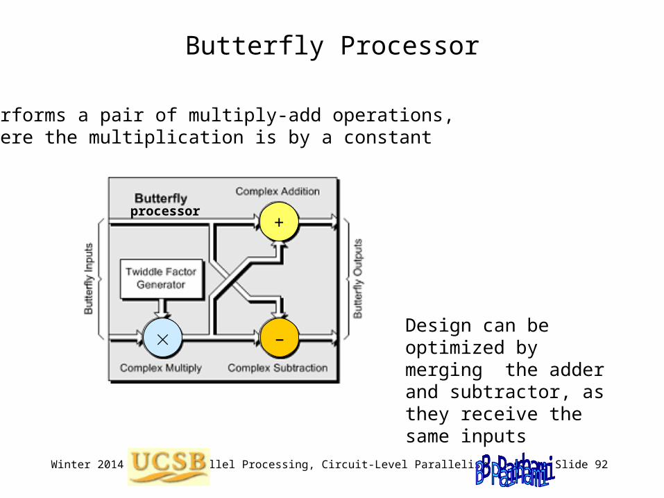
Butterfly Processor

Performs a pair of multiply-add operations, where the multiplication is by a constant

Design can be optimized by merging the adder and subtractor, as they receive the same inputs

processor+

–


Computation Scheme for 16-Point FFT0

1

2

3

4

5

6

7

8

9 10

11

12

13

14

15

0

1

2

3

4

5

6

7

8

9 10

11

12

13

14

15

Bit-reversal permutation

Butterfly operation

a b j

a + b a b

j j

0

0

0

0

0

0

0

0

0

4

0

4

0 4

0

4

0

2

4

6

0

2

4

6

0

1

2 3

4

5

6

7


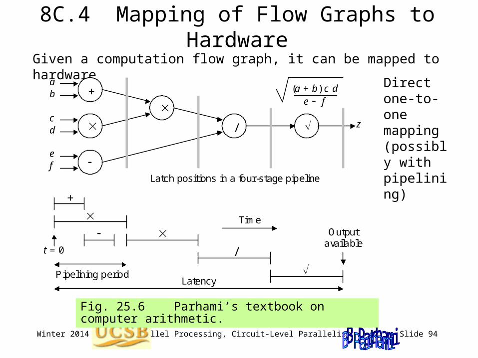
8C.4 Mapping of Flow Graphs to HardwareGiven a computation flow graph, it can be mapped to hardware

Direct one-to-one mapping (possibly with pipelining)

+

/

/

+

Pipelining period Latency

t = 0

Latch positions in a four-stage pipeline

a b

c d

e f

z

Output available

Time

(a + b) c d e f

Fig. 25.6 Parhami’s textbook on computer arithmetic.


Ad-hoc Scheduling on a Given Set of Resources

Given a computation flow graph, it can be mapped to hardware

Assume: tadd = 1tmult = 3tdiv = 8tsqrt = 10

+

/

/

+

Pipelining period Latency

t = 0

Latch positions in a four-stage pipeline

a b

c d

e f

z

Output available

Time

(a + b) c d e f

Add

Mult

Div /Sqrt

Time

+

–

0 1 2 3 6 14 24


Mapping through Projection

Given a flow graph, it can be projected in various directions to obtain corresponding hardware realizations

Multiple nodes of a flow graph may map onto a single hardware node

That one hardware node then performs the computations associated with the flow graph nodes one by one, according to some timing arrangement (schedule)

x0

x4

x2

x6

x1

x5

x3

x7

u0

u1

u2

u3

v0

v1

v2

v3

y0

y1

y2

y3

y4

y5

y6

y7

x0 u0

u2

u1

u3

v0

v2

v1

v3

y4

y2

y6

y1

y5

y3

y7x7

y0

x1

x2

x3

x4

x5

x6

Projection direction

Linear array, with each cell acting for one butterfly network row


8C.5 The Shuffle-Exchange Network

x0

x4

x2

x6

x1

x5

x3

x7

u0

u1

u2

u3

v0

v1

v2

v3

y0

y1

y2

y3

y4

y5

y6

y7

x0 u0

u2

u1

u3

v0

v2

v1

v3

y4

y2

y6

y1

y5

y3

y7x7

y0

x1

x2

x3

x4

x5

x6


Fig. 8.12 FFT network variant and its shared-hardware realization.

Variants of the Butterfly Architecture

x0 u0

u2

u1

u3

v0

v2

v1

v3

y4

y2

y6

y1

y5

y3

y7x7

y0

x1

x2

x3

x4

x5

x6


8C.6 Other Mappings of the FFT Flow Graph

This section is incomplete at this time


More Economical

FFT Hardware

Fig. 8.13 Linear array of log2n cells for n-point FFT computation.

x 0 u 0

u 2

u 1

u 3

v 0

v 2

v 1

v 3

y 4

y 2

y 6

y 1

y 5

y 3

y 7x 7

y 0

x 1

x 2

x 3

x 4

x 5

x 6

Project

Project

P ro je c t

P ro je c t

0

1

1

0

C o n tr o l

x

b

a

a b

a + b

n

i

y


Space-Time Diagram for the Feedback FFT Array

Feedbackbutterfly processor

winter 2014parallel processing, circuit-level parallelismslide 1 part ii circuit-level parallelism...

Documents

circuitlevel parallelismslide

design of sorting networks

classes of sorting networks

batcher sorting networks

sorting network correct

selection networks chapter

parallel inputs implementation

ninput sorting network