wireless power hotspot that charges all of your · pdf filewireless power hotspot that charges...

Wireless Power Hotspot that Charges All of Your Devices

Lixin Shi, Zachary Kabelac, Dina Katabi, David PerreaultMassachusetts Institute of Technology

Cambridge, MA, USA{lixin, zek, dina}@csail.mit.edu, [email protected]

ABSTRACTEach year, consumers carry an increasing number of gadgets on

their person: mobile phones, tablets, smartwatches, etc. As a result,users must remember to recharge each device, every day. Wirelesscharging promises to free users from this burden, allowing devicesto remain permanently unplugged. Today’s wireless charging, how-ever, is either limited to a single device, or is highly cumbersome,requiring the user to remove all of her wearable and handheld gad-gets and place them on a charging pad.

This paper introduces MultiSpot, a new wireless charging tech-nology that can charge multiple devices, even as the user is wearingthem or carrying them in her pocket. A MultiSpot charger acts as anaccess point for wireless power. When a user enters the vicinity ofthe MultiSpot charger, all of her gadgets start to charge automati-cally. We have prototyped MultiSpot and evaluated it using off-the-shelf mobile phones, smartwatches, and tablets. Our results showthat MultiSpot can charge 6 devices at distances of up to 50 cm.

CATEGORIES AND SUBJECT DESCRIPTORS

C.2.2 [Computer Systems Organization]: Computer-Communications Networks

KEYWORDS

Wireless Power Transfer; MIMO; Magnetic Resonance; Energy;Beamforming; Mobile and Wearable Devices

1. INTRODUCTIONOur daily lives rely on a multitude of personal mobile devices,

such as phones, tablets, and wearables. While every new devicehas made our lives easier in many respects, having to rememberand manage to charge all of our mobile devices is a recurring andincreasingly significant burden. If we could wirelessly charge ourdevices, it would alleviate this daily anxiety, and may even allowsuch devices to be permanently unplugged. While previous workhas taken initial steps towards this goal, it remains limited to a sin-gle device at a time [1, 2, 3], or is highly cumbersome requiring theuser to remove all of her wearable and handheld gadgets and placethem on a charging pad [4, 5], as in Fig. 1a.

Permission to make digital or hard copies of all or part of this work for personal orclassroom use is granted without fee provided that copies are not made or distributedfor profit or commercial advantage and that copies bear this notice and the full citationon the first page. Copyrights for components of this work owned by others than ACMmust be honored. Abstracting with credit is permitted. To copy otherwise, or republish,to post on servers or to redistribute to lists, requires prior specific permission and/or afee. Request permissions from [email protected]’15, September 07–11, 2015, Paris, France.c© 2015 ACM. ISBN 978-1-4503-3619-2/15/09 ...$15.00.

DOI: http://dx.doi.org/10.1145/2789168.2790092.

Imagine, however, if one had a single wireless charger that wasable to charge all of its surrounding devices simultaneously, evenif they were on the user’s body or in her purse. In some sense, thiswould emulate a miniature WiFi hotspot –i.e., the wireless chargerwould act as a power access point; once the user is in the vicin-ity of the charger, her devices start receiving power as needed,and if she moves away the charging stops. One could use sucha charger as a desk mat. Whenever the user sits at her desk, theiPhone in her pocket, the tablet in her purse, and the smartwatchon her wrist would charge automatically without even thinking ofthem, as shown in Fig. 1b.

But how can one deliver a wireless power hotspot? As we investi-gate the answer to this question, we focus on charging via magneticcoupling because it is the approach adopted by the wireless charg-ing standards [6, 7] and all consumer wireless charging products,and is deemed safe and compliant with FCC rules [8].1 In mag-netic coupling, the power transmitter uses one or more coils. Whenan AC current traverses the transmitter’s coil, it creates a variablemagnetic field. If this magnetic field traverses a nearby coil, it gen-erates an electric current, hence delivering power to that device. Thestronger the magnetic field is at the receiver, the more power is de-livered. The challenge, however, is that the magnetic field dies veryquickly with distance, and hence typical wireless charging devicesoperate at a very short distance of a couple of centimeters [6, 15].

Last year however, a MobiCom paper proposed a solution calledMagMIMO [1], where multiple coils on the transmitter act as amulti-antenna system, shaping the magnetic field in a beam andfocusing it on the receiver, in a manner similar to beamforming inMIMO systems.2 The paper demonstrated that for a single receiver,beamforming of the magnetic field can increase the charging rangeup to 40 cm and allow for a flexible phone orientation. Motivatedby this recent development, we investigate whether one can chargemultiple receivers at distance by shaping the magnetic field in mul-tiple beams focused on the various receivers.

At first blush, it might seem that one can beamform the mag-netic field to multiple receivers by directly borrowing from multi-user MIMO. Unfortunately, there is an intrinsic difference betweenmulti-user MIMO in RF communications and the physics of wire-less charging. Specifically, consider the effect of introducing mul-

1In particular, we use magnetic resonance [7]. Some start-ups haveadvocated the use of RF radiation [9, 10], ultrasound [11], orlasers [12] for wireless power transfer. None of those approacheshave made it into the standards for consumer electronics. Further,charging consumer electronics, e.g., phones, using RF or lasersraises safety concerns [13, 14] (for further details see §2).2The term “magnetic beamforming” in [1] and this paper refers toshaping the magnetic flux in the near field in the form of a beam(or multiple beams). In contrast, traditional beamforming in wire-less communication systems operates over radiated waves in the farfield.

2015 Annual International Conference on Mobile Computing (Mobicom ‘15), Sept. 2015 (to appear)

Wireless�Power�

Hotspot

(a) Today’s Wireless Charging (b) MultiSpot Charging Hotspot

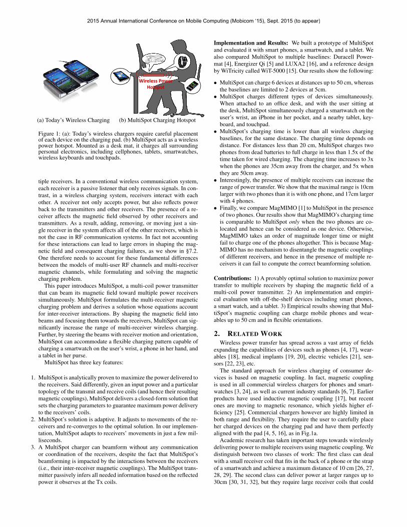
Figure 1: (a): Today’s wireless chargers require careful placementof each device on the charging pad. (b) MultiSpot acts as a wirelesspower hotspot. Mounted as a desk mat, it charges all surroundingpersonal electronics, including cellphones, tablets, smartwatches,wireless keyboards and touchpads.

tiple receivers. In a conventional wireless communication system,each receiver is a passive listener that only receives signals. In con-trast, in a wireless charging system, receivers interact with eachother. A receiver not only accepts power, but also reflects powerback to the transmitters and other receivers. The presence of a re-ceiver affects the magnetic field observed by other receivers andtransmitters. As a result, adding, removing, or moving just a sin-gle receiver in the system affects all of the other receivers, which isnot the case in RF communication systems. In fact not accountingfor these interactions can lead to large errors in shaping the mag-netic field and consequent charging failures, as we show in §7.2.One therefore needs to account for these fundamental differencesbetween the models of multi-user RF channels and multi-receivermagnetic channels, while formulating and solving the magneticcharging problem.

This paper introduces MultiSpot, a multi-coil power transmitterthat can beam its magnetic field toward multiple power receiverssimultaneously. MultiSpot formulates the multi-receiver magneticcharging problem and derives a solution whose equations accountfor inter-receiver interactions. By shaping the magnetic field intobeams and focusing them towards the receivers, MultiSpot can sig-nificantly increase the range of multi-receiver wireless charging.Further, by steering the beams with receiver motion and orientation,MultiSpot can accommodate a flexible charging pattern capable ofcharging a smartwatch on the user’s wrist, a phone in her hand, anda tablet in her purse.

MultiSpot has three key features:

1. MultiSpot is analytically proven to maximize the power delivered tothe receivers. Said differently, given an input power and a particulartopology of the transmit and receive coils (and hence their resultingmagnetic couplings), MultiSpot delivers a closed-form solution thatsets the charging parameters to guarantee maximum power deliveryto the receivers’ coils.

2. MultiSpot’s solution is adaptive. It adjusts to movements of the re-ceivers and re-converges to the optimal solution. In our implemen-tation, MultiSpot adapts to receivers’ movements in just a few mil-liseconds.

3. A MultiSpot charger can beamform without any communicationor coordination of the receivers, despite the fact that MultiSpot’sbeamforming is impacted by the interactions between the receivers(i.e., their inter-receiver magnetic couplings). The MultiSpot trans-mitter passively infers all needed information based on the reflectedpower it observes at the Tx coils.

Implementation and Results: We built a prototype of MultiSpotand evaluated it with smart phones, a smartwatch, and a tablet. Wealso compared MultiSpot to multiple baselines: Duracell Power-mat [4], Energizer Qi [5] and LUXA2 [16], and a reference designby WiTricity called WiT-5000 [15]. Our results show the following:

• MultiSpot can charge 6 devices at distances up to 50 cm, whereasthe baselines are limited to 2 devices at 5cm.• MultiSpot charges different types of devices simultaneously.

When attached to an office desk, and with the user sitting atthe desk, MultiSpot simultaneously charged a smartwatch on theuser’s wrist, an iPhone in her pocket, and a nearby tablet, key-board, and touchpad.• MultiSpot’s charging time is lower than all wireless charging

baselines, for the same distance. The charging time depends ondistance. For distances less than 20 cm, MultiSpot charges twophones from dead batteries to full charge in less than 1.5x of thetime taken for wired charging. The charging time increases to 3xwhen the phones are 35cm away from the charger, and 5x whenthey are 50cm away.• Interestingly, the presence of multiple receivers can increase the

range of power transfer. We show that the maximal range is 10cmlarger with two phones than it is with one phone, and 17cm largerwith 4 phones.• Finally, we compare MagMIMO [1] to MultiSpot in the presence

of two phones. Our results show that MagMIMO’s charging timeis comparable to MultiSpot only when the two phones are co-located and hence can be considered as one device. Otherwise,MagMIMO takes an order of magnitude longer time or mightfail to charge one of the phones altogether. This is because Mag-MIMO has no mechanism to disentangle the magnetic couplingsof different receivers, and hence in the presence of multiple re-ceivers it can fail to compute the correct beamforming solution.

Contributions: 1) A provably optimal solution to maximize powertransfer to multiple receivers by shaping the magnetic field of amulti-coil power transmitter. 2) An implementation and empiri-cal evaluation with off-the-shelf devices including smart phones,a smart watch, and a tablet. 3) Empirical results showing that Mul-tiSpot’s magnetic coupling can charge mobile phones and wear-ables up to 50 cm and in flexible orientations.

2. RELATED WORKWireless power transfer has spread across a vast array of fields

expanding the capabilities of devices such as phones [4, 17], wear-ables [18], medical implants [19, 20], electric vehicles [21], sen-sors [22, 23], etc.

The standard approach for wireless charging of consumer de-vices is based on magnetic coupling. In fact, magnetic couplingis used in all commercial wireless chargers for phones and smart-watches [3, 24], as well as current industry standards [6, 7]. Earlierproducts have used inductive magnetic coupling [17], but recentones are moving to magnetic resonance, which yields higher ef-ficiency [25]. Commercial chargers however are highly limited inboth range and flexibility. They require the user to carefully placeher charged devices on the charging pad and have them perfectlyaligned with the pad [4, 5, 16], as in Fig.1a.

Academic research has taken important steps towards wirelesslydelivering power to multiple receivers using magnetic coupling. Wedistinguish between two classes of work: The first class can dealwith a small receiver coil that fits in the back of a phone or the strapof a smartwatch and achieve a maximum distance of 10 cm [26, 27,28, 29]. The second class can deliver power at larger ranges up to30cm [30, 31, 32], but they require large receiver coils that could


not possibly fit on the back of a phone or wearable. In addition, bothclasses assume the receiver coil is aligned with the transmitter coil,and do not deal with different receiver orientations with respect tothe transmitter. In practice, however, the user cannot benefit from anincrease in charging distance if she has to hold her device on top ofthe charging pad and maintain a perfect alignment with the charger.MultiSpot is unique in that it adapts the shape of the magnetic fieldaccording to the location and orientation of the receivers by con-structively combining the magnetic fields of multiple Tx coils. Thisallows MultiSpot to reduce the size of the receiver coil to fit onphones and wearables, while supporting larger ranges and flexiblereceiver orientations.

Researchers have also explored using multiple transmit coils tobeamform the magnetic field to receivers. In fact, MultiSpot is in-spired by MagMIMO’s techniques [1]. However, as described ear-lier in Sec. §1, MagMIMO does not work in the presence of morethan one receiver, while MultiSpot is designed to work with anynumber of receivers. We show in experiments (Sec.§7) that whentwo receivers are separated from each other, MagMIMO cannotcharge them.

Very recently, another work was accepted for publication, whichalso uses multiple transmit coils, and examines the possibility ofcombining their fields at up to 2 receivers [33]. While the workdemonstrates the potential of multi-user charging, it presents an op-timal solution only for a single receiver, and uses brute force explo-ration to determine the optimal solution for two receivers. Further,the work presents an implementation only for the single receivercase, and uses simulation for the two-receiver case. In contrast,MultiSpot presents an optimal solution for any number of receivers.Further, MultiSpot is implemented and empirically evaluated for upto 6 receivers.

We also note that there have been recent proposals of wirelesscharging using physical phenomena other than magnetic coupling.Ultrasound [11], lasers [12], and power delivery via RF radiation [9,10] have been proposed by startup companies. However, none ofthese companies have published their technologies nor offered aproduct. Furthermore, ultrasound charging is limited to line-of-sight scenarios and will be disrupted if the phone is not directly infront of the charger [34]. It can also negatively affect pets who hearsome types of ultrasound [35]. Lasers can cause damage to one’seyesight [13], and delivering power to mobile devices via RF radi-ation at hundreds of MHz to GHz heats up water which composesmost of a human body, similarly to how a microwave oven cooksfood [14].3 Beyond the safety problems, it is also unclear how thesetechnologies can be compliant with FCC regulations.

3. PRIMERIn this section, we explain how magnetic coupling works at a

high level. In this approach, the transmitter coil is driven by an ACcurrent to generate an oscillating magnetic field. When another con-ductive coil is placed within range of the transmitter, some of themagnetic field passes through the center of its coil. This field in-duces an AC current on the receiver, which can be used to powerthe device.

To boost the efficiency of power transfer, state-of-the-art systemsand industrial standards [6, 7], use a technique called magnetic res-

3To see how delivering power via RF radiation to a phone mightbe dangerous, let us do a rough calculation. Say that a standardphone requires at least 1W to turn on charging, and it has an areaof 5cm×10cm, i.e., the power density is 20mW/cm2. As a com-parison, FDA (Food and Drug Administration) enforces microwaveoven leakage to be below 5mW/cm2 in order to be consideredsafe [36].

VT

IT

+

í

Tx

IR

Rx

LT LR

CTCR

M

ZT

ZR

Figure 2: Single-Coil Tx, Single Rx Schematic

onance [25], in which they add a capacitor to the transmitter andreceiver circuits and make them resonate at the same frequency.The oscillations cause the circuits to resonate back and forth with-out consuming much energy. Magnetic resonance is the underlyingpower transfer mechanism used in MultiSpot.

3.1 Circuit EquationsMagnetic coupling and the resulting power transfer can be math-

ematically described via basic circuit equations [37].

Single Coil System: Consider the system in Fig. 2, which shows asingle coil transmitter and a single receiver. Let us write the equa-tions that describe this system. As we do so, we will take into ac-count that in magnetic resonance, the inductance and capacitor arechosen so that their impacts cancel each other at the resonant fre-quency (i.e., jωL+ 1

jωC= 0). Thus, we can ignore those terms.

We can describe the system in Fig. 2 using two equations. Thefirst equation determines how a current in the transmit coil, IT ,induces a current in the receive coil, IR, i.e.:

ZRIR = jωMIT (1)

whereM is the magnetic coupling between the transmit and receivecoils, ZR is the impedance of the receiver and ω is the resonantfrequency.

The above equation would have been sufficient to describe thesystem if one could directly apply a current to the transmit coil.Unfortunately, in practice, one has to use a voltage source instead.Thus, we need a second equation that determines the relationshipbetween the voltage one applies to the transmitter, VT and the re-sulting transmitter current, IT .

For the circuit in Fig. 2, we have: VT = ZT IT −jωMIR, whereZT represents the impedance in the transmitter. Note in this equa-tion how the current in the receiver induces a voltage back on thetransmitter via the same magnetic couplingM . We can further sub-stitute IR from Eq. (1) to obtain:

VT =(ZT + ω2M2/ZR

)IT . (2)

Together Eq. (1) and Eq. (2) describe the single-coil chargingsystem.

Multi-Coil System: The above two equations can be generalizedto the case of multiple transmitter coils and multiple receiver coils,shown in Fig. 3a. The difference is that now every pair of coilshas magnetic coupling between them. Specifically, there are threetypes of couplings: MTik between transmitter i and k, Miu be-tween transmitter i and receiver u, and MRuv between receiver uand v.

We can update Eq. (1) and Eq. (2) to account for the additionalcoupling between transmitter coils, and between receiver coils. Re-


Tx iRx u

LTi

Miv

IRu

LRu

CRu

+

í

VTi

ITi

CTi

+

í

VTk

ITk

CTk

Mju

Tx k

LTk

MTij

IRv

LRv

CRv

Rx v

Mjv

Miu

MRuv

ZTi

ZTk

ZRu

ZRv

(a) Multi-coil Tx, Multiple Rx Schematic

Term Definition Explanationn Number of Tx coilsm Number of Rx coils~vT [VT1, VT2, · · · , VTn]>n×1 Tx voltages~iT [IT1, IT2, · · · , ITn]>n×1 Tx currents~iR [IR1, IR2, · · · , IRm]>n×1 Rx currents

ZR

ZR1 jωMR12 · · · jωMR1m

jωMR21 ZR2 · · · jωMR2m

......

. . ....

jωMRm1 jωMRm2 · · · ZRm

m×m

Rx impedanceand inter-Rx

magnetic couplings

ZT

ZT1 jωMT12 · · · jωMT1n

jωMT21 ZT2 · · · jωMT2n

......

. . ....

jωMTn1 jωMTn2 · · · ZTn

n×n

Tx impedanceand inter-Tx

magnetic couplings

M

M11 M21 · · · Mn1

......

. . ....

M1m M2m · · · Mnm

m×n

Tx-Rxmagnetic couplings

(b) Matrix & Vector Denotations

Figure 3: Circuit Schematic and Denotations of a Multi-Coil Tx, Multiple Rx Wireless Power Delivery System

ceiver u’s circuit equation becomes:

ZRuIRu +∑v 6=u

jωMRuvIRv︸︷︷︸from the other receivers

=∑i

jωMiuITi︸︷︷︸from the transmitters

(3)

while the transmitter voltage at coil i is:

VTi = ZTiITi +∑k 6=i

jωMTikITk︸︷︷︸from the other transmitters

−∑u

jωMiuIRu︸︷︷︸from the receivers

(4)

For convenience, we rewrite Eq. (3) and (4) in matrix form:

Rx Equation: ~iR = jωZ−1R M

~iT (5)

Tx Equation: ~vT =(ZT + ω2M>Z−1

R M)~iT (6)

where the matrix and vector denotations are defined in Table 3b.4

Eq. (5) and Eq. (6) are sufficient to describe the multi-coil systemin Fig. 3a. Specifically, Eq. (5) describes what receiver current ~iRwe will get if a transmitter current~iT is applied, thus we call it theReceiver Equation. Eq. (6), on the other hand, shows what voltage~vT we need to apply in order to obtain transmitter currents ~iT , sowe name it the Transmit Equation. These two equations describe themost fundamental relationships in our multi-Tx multi-Rx system,and are the basis of all of the following conclusions of MultiSpot.

4. MULTISPOTMultiSpot is a new technology for charging multiple devices

wirelessly via magnetic resonance. It uses multiple transmit coils,which could be built into a desk mat to deliver a user experienceanalogous to a mini hotspot –i.e., when the user sits at her desk,all of her electronic gadgets start receiving power automatically.MultiSpot’s design is mainly focused on the transmitter side. Thereceiver design follows that of standard wireless charging circuits,which can be built into the sleeve of a phone or the strap of a smart-watch.

4Note that similar to the single-Tx single-Rx case, Eq. (6) is ob-tained by first rewriting Eq. (4) into ~vT = ZT~iT − jωM>~iR andthen substituting~iR using Eq. (5).

At first blush, it might seem that one can build a wireless powerhotspot by beamforming the magnetic field to one receiver at atime using MagMIMO [1], and iterating between receivers usinga TDMA style MAC. Unfortunately MagMIMO intrinsically as-sumes only one receiver. If multiple receivers are nearby, they allcouple with each other and the transmitter coils. As a result, Mag-MIMO cannot discover the coupling due to each receiver (i.e., themagnetic channel to the receiver [1]) and hence cannot computethe beamforming parameters correctly. In fact MagMIMO wouldnot know whether there is a single or multiple receivers. One couldalso try to add out-of-band communication (via WiFi or Bluetooth)to coordinate receivers, turn some receivers off so that at any pointin time there is coupling only from one receiver, synchronize thereceivers as they turn on and off, and have receivers detect any mo-tion and inform each other so that they may re-estimate coupling.Such an approach is excessively complex and high overhead, and isnot even clear how one can extend this idea into a full system.

Below we describe a design that requires neither receiver coordi-nation nor out-of-band communication. It operates entirely on thetransmitter allowing it to shape the magnetic field in multiple beamsfocused on the receivers, in a manner that is analytically proven tomaximize power delivery.

4.1 Optimizing Power Delivery to ReceiversIn wireless communication systems, such as MU-MIMO, beam-

forming effectively combines the signals constructively at the re-ceivers so that the received signal gets maximized. This is achievedby carefully setting the transmitter signal according to the wirelesschannels. Similar concepts can be applied to wireless power deliv-ery systems. However, to beamform in MultiSpot, we need to an-swer two questions. What exactly are the “signals” and “channels”?And how do we maximize the power of the received signal?

(a) Magnetic Channel: The Receiver Eq. (5) provides us a way toanalogously define magnetic channels. Specifically, if we analogizecurrents to signals, the transmitted and received signals will be ~iTand ~iR. Therefore, the coefficient between them is the magneticchannel, i.e.:

~iR = H~iT , whereH = jωZ−1R M (7)

Note that the magnetic channel H is different from the channelmatrix in MU-MIMO, where it is simply a concatenation of in-


dividual channels between every pair of transmitter and receiver.Rather, in MultiSpot, it is the multiplication of two parts: H =HRx−RxHRx−Tx where HRx−Rx = Z−1

R contains receiver-receiver couplings and HRx−Tx = jωM contains transmitter-receiver couplings. Physically, these two sub-channel matrices de-scribe two processes that occur in multi-TX-coil multi-receiverpower transfer system: HRx−Tx characterizes the induced poweron the receivers from transmitters, whileHRx−Rx captures the re-distribution of transmitted power among receivers due to receiver-receiver coupling.

(b) Maximizing Received Power: The challenge becomes howto set the transmitter signals, (i.e., ~iT ), so that the received poweris maximized. This question can be formulated as an optimizationproblem that maximizes the received power PR, under the con-straint of a total input power P .

The received power PR can be written as the summation of thepower delivered to each receiver, i.e.:

PR = ~i∗RRR

~iR, (8)

where ~iR is a vector of the receiver currents. The superscript (∗)denotes conjugate transpose, and RR is a diagonal matrix whoseentries are the resistances of each receiver.5

The input power can be written as the total power dissipated onthe transmitter and receivers, i.e., P = PR + PT . This is becausepower does not disappear, and hence must either be delivered to thereceivers, or be consumed on the transmitters. Thus:

P = PR + PT = ~i∗RRR

~iR +~i∗TRT

~iT , (9)

where RR and RT are diagonal matrices of transmitter and re-ceiver resistances.

Now, we can re-write the optimization problem that maximizespower transfer by substituting the received power and the inputpower by their values from Eq. (8) and Eq. (9). We also substitutethe received currents from Eq. (7),~iR = H~iT . Thus, our optimiza-tion problem becomes: Find the transmit currents that satisfy:

~ibfT = arg max

{~i∗TH

∗RRH~iT}

conditioned on: ~i∗TRT

~iT +~i∗TH

∗RRH~iT = P,(10)

where~ibfT denotes the set of currents that beamforms.

In Appendix A, we prove that the solution to this optimizationis:

THEOREM 4.1. The following transmitter current vector willmaximize the received power:

~ibfT = c · maxeig(H∗RRH) (11)

where maxeig (H∗RRH) is the eigenvector ofH∗RRH that cor-responds to the largest real eigenvalue λ, and c is a normalizationscalar defined in App. A. Specifically, the maximal delivered poweris equal to λ

λ+1P .

This theorem guarantees that MultiSpot maximizes the power de-livered from the transmitter coils to the receiver coils. This meansthat for the same hardware and any given relative locations of trans-mitter and receiver coils, no other algorithm can deliver more powerthan what is specified by the theorem.

(c) Applying the Beamforming Solution: The solution fromThm. 4.1 would be sufficient if one could directly apply the cur-rents to the coil. However, in practice, one has to use a voltage5If a receiver is not fully resistive, i.e., its impedance ZRu has animaginary component, then RRu = Real(ZRu).

source instead. Therefore, we need to convert these currents to theircorresponding voltages so that they are directly applicable to the Txcoils via standard voltage sources.

Fortunately, the Transmitter Eq. (6) that relates transmitter cur-rents to voltages was derived in §3.1. Specifically, the set of volt-ages that we need to apply to the Tx coils is:

~vbfT =

(ZT + ω2M>Z−1

R M)~ibfT . (12)

In summary, maximizing power delivery requires two steps:

1. Calculate the beamforming currents,~ibfT .

2. Convert the currents to voltages by ~vbfT , and apply the voltages to

the transmitter coils.

4.2 Eliminating Need for Receivers’ CommunicationIn the previous section, we showed how a MultiSpot charger

could beamform. However, two steps are needed to beamform, bothof which require information that resides on the receivers, and isunavailable at the transmitter.

• In the first step, the beamforming currents,~ibfT , are calculated via

Thm. 4.1, which is strictly dependent on knowing H∗RRH .Recall, however, that the channel contains receiver-receiver cou-plings, unknown to the transmitter.• In the second step, the beamforming voltages, ~vbf

T , are com-puted using Eq. (12), which depends on knowing (ZT +ω2M>Z−1

R M). ZT contains only transmitter specific param-eters (i.e., transmitter to transmitter couplings and impedances)and hence can be estimated a priori in a factory setting (for de-tails, see Appendix D). However, the matrix (ω2M>Z−1

R M)contains receiver-receiver couplings and receiver impedances.This matrix which we denote Y = ω2M>Z−1

R M is unknowna priori to the transmitter (and changes with time because thecoupling depends on receiver position).

Thus, beamforming requires estimating H∗RRH and Y , bothof which involve receiver dependent information. So, how can aMultiSpot transmitter estimate these matrices without explicit in-formation from the receivers?

Estimating Y : Let us first consider estimating Y . The Transmit-ter Eq. (6) can be rewritten as ~vT = (ZT + Y )~iT , where theonly unknown coefficient is Y because ZT is measured duringpre-calibration. By applying voltages and measuring the resultingcurrents on the Tx coils, we can estimate the coefficient betweenthem. Since both ~vT and ~iT are vectors of length n, we need torepeat the measurement process n times before applying matrix in-version, where n is the number of Tx coils. More formally, if oneapplies n different sets of voltages ~v(1)

T , · · · , ~v(n)T and measures the

corresponding currents~i(1)

T , · · · ,~i(n)

T , one can estimate Y by:

Y =[~v

(1)T ··· ~v(n)

T

]·[~i

(1)

T ··· ~i(n)

T

]−1

− ZT (13)

Estimating H∗RRH: After obtaining Y , we are still left withthe problem of estimatingH∗RRH . Recall thatH = jωZ−1

R M ,which means both transmitter-receiver couplings and receiver-receiver couplings need to be estimated. Unlike the matrix Y how-ever, which can be estimated at the transmitter using measurementsof ~vt and~iT , there is no way to measureH at the transmitter.

Fortunately, MultiSpot does not need to estimateH . Instead, weshow that a MultiSpot transmitter can estimate the matrix product


1 MultiSpot Algorithm

1: Y ← rand(n× n) �Y can be initialized to any matrix2: while true do3: ~ibf

T = c ·maxeig(Real(Y ))�compute beamforming currents

4: Apply ~vbfT =

(ZT + Y

)~ibfT �beamform

5: Measure~iT on the transmitter6: ∆~iT ← ~ibf

T −~iT7: if ∆~iT 6= ~0 then � if the channel changes

8: Y ← Y +∆~vT ∆~v>T∆~v>

T~iT

, where ∆~vT = (ZT + Y )∆~iT

� update Y9: end if

10: end while

H∗RRH as a whole; and it can do so completely passively. Fur-ther, we can relate H∗RRH to something we have already mea-sured, namely Y . Specifically, we prove in Appendix B the follow-ing theorem:

THEOREM 4.2. Define Real(·) as the real part of a matrix, then

H∗RRH = Real(Y ) (14)

whereH = jωZ−1R M and Y = ω2M>Z−1

R M .

Since we have already shown how to compute Y , the above the-orem allows us to computeH∗RRH by taking its real part.

Therefore, we have developed a method to estimate all neededparameters solely on the transmitter, without any communicationor feedback from the receivers.

4.3 Adaptive BeamformingNext, we would like to ensure that MultiSpot can smoothly adapt

to receiver motion and receivers entering and leaving the system.This is particularly important for wearable receivers which tend tobe highly dynamic, e.g., a smartwatch on a user’s wrist.

When receivers move (or are added/removed), the magnetic cou-plings change across all devices, leading to new values for H andY . One could address this problem by repeatedly estimating Y andH∗RRH , as explained in §4.2. This, however, would be subopti-mal since estimatingY from scratch requires the MultiSpot chargerto stop beamforming and apply other voltages in order to obtainenough measurements as required by Eq. (13). Furthermore, sincethe transmitter does not know when receivers move, it is left witha difficult choice: Either it can repeat the estimation infrequently,which would be inefficient in scenarios with lots of motion, or itcan repeat the estimation, often leading to frequent and unneces-sary interruptions in beamforming when the receivers are static.

In this section, we propose an adaptive algorithm, which we calladaptive beamforming, that addresses the conflict: It uninterrupt-edly beamforms whenever the receivers remain static, and seam-lessly and quickly adapts when any receiver moves.

The key idea is that instead of estimating Y from scratch, whichwould interrupt beamforming, the adaptive algorithm iterativelycomputes the new Y . In each iteration, the algorithm computesan incremental update to Y that satisfies the following two con-straints: 1) If no receiver moves, the update is zero; and 2) If anyreceiver moves, the update rule is guaranteed to move Y toward itstrue value and converge to the true value within a small number ofsteps.

Alg. 1 outlines MultiSpot’s adaptive beamforming. For clarity,we use Y to denote the algorithm’s estimate of the true Y matrix.

To start the algorithm randomly assigns an initial matrix to Y . Ineach iteration, the algorithm calculates the beamforming currentsand converts them to beamforming voltages, which it applies to thetransmitter coils.

Next (Line 5), the algorithm measures the currents on the trans-mit coils. If Y is accurate, the measured currents should be equalto the currents that beamform (~ibf

T ). Otherwise the algorithm usesthe mismatch between the measured and expected currents and theresulting mismatch in voltages to update its estimate of Y (Line 7).

It should be clear from the update rule in Line 7 that if noth-ing changes (e.g., no receiver moves), no update will occur and thebeamforming is unmodified. Further, the theorem below guaranteesthat when a change occurs, the algorithm quickly converges to theoptimal beamforming solution.

THEOREM 4.3. If Y 6= Y , then Alg. 1 is guaranteed to up-date Y to Y in less than n iterations, where n is the number oftransmitters.

Thm. 4.3 is formally proven in Appendix C. Thm. 4.3 not onlyproves convergence but it puts an upper bound on the time to con-vergence. The convergence time is bounded only by the number oftransmit coils, and is independent of the number of receivers. 6 Inour implementation where the transmitter uses a standard micro-controller, each iteration in Alg. 1 can be finished in less than 1ms.When there is any movement, the algorithm takes about 5ms to con-verge to the new set of channels. This speed is more than sufficientfor our application.

4.4 Power Distribution Among ReceiversThe previous section presents an algorithm that adaptively deliv-

ers maximal power to the receivers. But how does the solution dis-tribute this power among the various receivers? In order to gain in-sight into power distribution, we discuss three representative cases.

• In the first scenario, we consider identical receivers from the per-spective of wireless charging – i.e., receivers with the same bat-tery level, distance, and orientation with respect to the transmit-ter, and hence the same magnetic coupling. In this case, all re-ceivers are allocated equal amounts of power. This is because thesystem is symmetric with respect to the receivers and hence aneven power distribution yields the optimal solution.• In the second scenario, we consider receivers that have the same

battery level (i.e., the same demands for charging), but differ-ent magnetic couplings. Physically, this can be caused by somereceivers being placed closer to the transmitter than others, withmore favorable orientations, or simply having a larger coil. Eitherway, the receivers with stronger magnetic coupling will receivemore power. This property is similar in spirit to resource alloca-tion in typical networking systems. For example, TCP flows withshorter RTTs and WiFi clients with higher SNRs receive higherdata rates.• In the final case, we consider what happens as some receivers

approach a fully charged battery while others are still in needfor charging. We argue that in this case the MultiSpot chargernaturally reduces the power allocated to the more charged re-ceivers, diverting that power to those receivers who are still inneed for wireless power. Specifically, consider two receivers withthe same magnetic coupling, one of which is fully charged whilethe other has a low battery level.

6It is worth noting that a MultiSpot charger does not need to knowthe number of receivers to run Alg. 1. The charger has enough in-formation to infer the number of receivers, which is equal to therank of Y .


Tx 1

Tx 2

Tx n

Micro

Controller

Measurement Circuits

Power Converter

Power Converter

Power Converter

(a) Tx Diagram

Impedance

Matching

DC/DC

Regulator

Rx

AC/DC Rectifier

(b) Rx Diagram

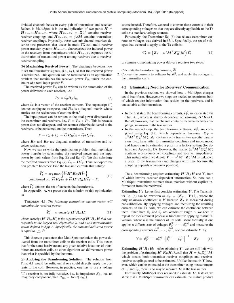
Figure 4: Circuit Diagram of MultiSpot’s Tx and Rx

When the battery is charged, the device needs very little powerso it does not accept current. In this case the receiver circuit canbe approximated by an open circuit, i.e., IR ≈ 0 for that re-ceiver [38]. As a result, the receiver does not reflect power to-ward the transmitter. Therefore, the MultiSpot transmitter willnot sense this receiver or beamform to it. In general, the progres-sion from accepting current when the receiver has low batterylevels to not accepting current when it is fully charged is grad-ual. Therefore, the algorithm gradually allocates less power todevices that are more charged.

To validate this intuition, we test each of the above situationsexperimentally in §7.

5. IMPLEMENTATIONWe have built a prototype of MultiSpot to charge electronics in

an office scenario. Our setup is similar to past work [1]. Specifi-cally, the transmitter is composed of 6 copper coils and is mountedto the bottom of an office desk. Each transmit coil covers an area of0.05m2, which collectively cover an area of 0.38m2. The transmit-ter can be attached to a regular office desk with metallic, plastic andwood contents. The only restriction of the system is that the desksurface must not be conductive.7 Each phone receiver contains asingle copper coil, of area 0.005m2, that is embedded into a sleevethat attaches to the back of the device. As for the smartwatch, weembed the coil into the band of the watch.

In our implementation, the transmitter and receivers resonate at1MHz, as in [1], which is within the frequency range of commonwireless charging systems [15, 6, 7]. In addition, the setup is com-patible with FCC regulations including part 15 and part 18.

The transmitter’s architecture is shown in Fig. 4(a). Mul-tiSpot drives 6 transmit coils to beamform a magnetic field towardsthe receivers. The output voltage and current of each coil are mea-sured by the measurement circuit. This circuit employs quadraturemixers, AD8333 [40], to acquire the phase and amplitude of eachsignal and output them to the microcontroller. The microcontrollerplatform, Zynq 7Z010 [41], takes as input these amplitudes andphases and runs MultiSpot’s algorithm. Every time Alg. 1 receivesnew measurements, it updates its estimates accordingly, and calcu-lates the new voltages needed to beamform. It then sends the newset of voltages to the controller circuits which apply them to thetransmit coils using a Class D Full Bridge Power Converter [42].7Conductive materials as large as the desk surface might negativelyaffect MultiSpot’s performance. This is a standard assumption re-quired by magnetic wireless power delivery and can be found inresearch papers [1] and commercial systems [39].

This converter allows the controller circuit to flexibly control boththe amplitudes and phases of the voltages applied to the transmitcoils.

The receiver circuit is shown in Fig. 4(b). It has an impedancematching network designed to maximize the power that gets deliv-ered to the device. This is followed by a full bridge rectifier whichconverts the AC signal into a DC voltage. This DC voltage passesthrough a DC-DC voltage regulator that converts the input voltageto a constant 5V. This allows the power to be distributed across aUSB port so that the receiver can support a large variety of unmod-ified devices that can be charged via USB, including most phones,tablets and wearables.

6. EVALUATION ENVIRONMENT

Metrics: We define distance as the distance between the nearestpoint on the receiver coil and the transmitter coils. For example, ifa receiver is in the same plane of the transmitter but outside the areathat the transmitter coils cover, then the distance is from the edgeof the receiver to the edge of the nearest transmitter coil.

We define charging time ratio as the ratio between the time takento wirelessly charge a phone from dead to full battery, to the time ittakes a wall plug to do the same. For multiple phones, the chargingtime ratio reported is the largest time ratio of all involved phones,i.e., it is the charging time of the phone that takes longest to charge.

We define orientation as the angle between the plane of the re-ceiver coil and the plane of the transmitter coils.

Baselines: We compare the following systems:

• Commercially available multi-device wireless chargers: Dura-cell Powermat [4], Energizer Qi [5] and LUXA2 [16]. Each ofthem requires a proprietary receiving case, which we attach tothe phone during the experiments.• State-of-the-art Prototype. Specifically, we choose the WiTricity

WiT-5000 prototype [15] that charges multiple devices. Since theprototype is not publicly available, we extract the data from theirtechnical sheet [15].• Idealized Selective Coil: This baseline uses the same 6 Tx coils

as MultiSpot, but given a set of receivers, it identifies the bestTx coil for each receiver, and divides the input power equally be-tween the set of best Tx coils. For example, given two receivers,it identifies the best Tx coil for the first receiver, and the best Txcoil for the second receiver, and divides the power between thosetwo Tx coils.We note that this baseline requires an oracle to decide which Txcoil would deliver the maximum power to each receiver. Specif-ically, one cannot identify the Tx coil that has the best magneticcoupling to a receiver in the presence of other receivers. Hence,to implement this system, for each receiver, we physically re-move the other receivers and measure the receiver coupling tothe transmitter. While this is hard to do in a real-world setup,the baseline provides insights about how well one can do by dis-tributing the input power between the best performing Tx coils.• Our MultiSpot prototype described in §5.• MagMIMO [1] using the same Tx coils as MultiSpot.

We note that the input powers of Duracell Powermat [4], Ener-gizer Qi [5], LUXA2 [16], and WiTricity WiT-500 [15] are 15W,18W, 22W, and 24W, respectively. Since these baselines have dif-ferent input powers, we set the input power of MultiSpot, selectivecoil, and MagMIMO to the mean of those values, i.e., 20W.

Setup: All experiments are performed in an office environment.The charger is placed on a standard office desk. Unless specifiedotherwise, the charged devices (e.g., phones) are held using config-


0

1

2

3

4

5

6

7

8

0 10 20 30 40 50

Charg

ing T

ime R

atio

Distance (cm)

MultiSpot

IdealizedSelective

Coil 1

1.5

2

0 2 4

Energizer

LUXA2

Duracell

WiT-5000

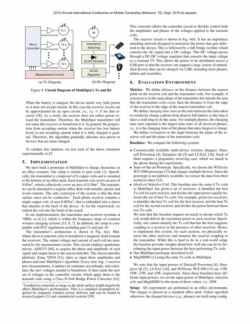
Figure 5: Charging Time Ratio vs. Distance from Charger. Eachrun uses 2 phones at equal distance, but in different locations.

1

2

3

4

5

6

7

8

9

Scenario 1 Scenario 2 Scenario 3

Charg

ing T

ime R

atio

NOTCharging

MultiSpotMagMIMO

Figure 6: Comparison with MagMIMO: Scenario 1: two re-ceivers 5cm apart and both 25cm away from the transmitter; Sce-nario 2: two receivers 60cm apart and both 10cm away from thetransmitter; Scenario 3: two receivers 60cm apart and both 20cmaway. The figure shows that MagMIMO works well for co-locatedreceivers, but can completely fail if the receivers are far apart.

urable arms which allows us to test different charging distances andorientations.

7. RESULTS

7.1 Charging Time vs. DistanceWe evaluate MultiSpot’s ability to charge multiple phones at var-

ious distances from the transmitter. We run each experiment with 2phones because the commercial baselines are constrained to charg-ing 2 receivers. The distance of both receivers is increased from2cm to 50cm together. At each distance, multiple experiments arerun with different receiver positions and orientations.

Fig. 5 shows the charging time ratio of MultiSpot and the base-lines as a function of the distance from the charger. At near dis-tances (0-10cm), MultiSpot’s charging time is comparable to awired charger. It starts to increase at mid-range to far-range. Mul-tiSpot reaches as far as 50cm. Comparing with the baselines, Mul-tiSpot has much larger range, and shorter charging time at thesame range. The commercial baselines (Energizer, LUXA2, Du-racell) and development prototype (WiT-5000) are constrained toless than 5cm. Even when compared to the idealized selective-coil,MultiSpot reaches much larger range. And even within the samerange, MultiSpot’s charging time is on average 3x smaller than thatof idealized selective coil.

7.2 Comparison with MagMIMOMultiSpot is inspired by MagMIMO [1], which proposes mag-

netic beamforming to a single device. Thus, in this experiment

0

1

2

3

4

− − − | | | / \

Ch

arg

ing

Tim

e R

atio

Rx 1Rx 2

Figure 7: Charging Time vs. Orientation. We plot the chargingtime ratio versus different orientations. Each group of two bars rep-resent a combination of orientations, where “−” denotes horizontal,“|” denotes vertical, while “/” and “\” denote 45◦. All receivers are25cm away from the charger.

we compare MagMIMO with MultiSpot. We separate this exper-iment from the other baselines since MagMIMO is not intended forcharging multiple devices. Still one might wonder how MagMIMOwould perform when there are multiple devices around, and howdoes it compare to MultiSpot.

We use the same hardware to run MultiSpot and MagMIMO. Weuse two receivers and run both MagMIMO and MultiSpot in threedifferent scenarios. In the first scenario, the two receivers are co-located within 5cm from each other, and both are 25cm away fromthe transmitter. In the second scenario, the receivers are 60cm apart,and both 10cm away from the transmitter. In the third scenario,the two receivers are 60cm apart and both 20cm away from thetransmitter.

Fig. 6 shows that MagMIMO is comparable to MultiSpot onlywhen the two phones are co-located and hence can be considered asone device. Otherwise, MagMIMO’s charging time becomes an or-der of magnitude longer than MultiSpot, or it fails to charge one ofthe phones all together. The reason is that MagMIMO has no mech-anism for separating the magnetic couplings of the two receivers,and hence interprets the magnetic channels of both receivers as onechannel and tries to create one beam to charge both phones. Whenthe phones are adjacent, this technique works because one beamcan charge both receivers, but as this distance increases, the charg-ing time ratio inevitably goes up. MultiSpot on the other hand, cre-ates two beams for both receivers and is able to power both phonesregardless of the distance between them.

7.3 Charging Time vs. OrientationWe investigate MultiSpot’s performance with different receiver

orientations. For all experiments, the distances of both receivers isfixed to be 25cm, while their orientations are varied. We test fourscenarios: both phones horizontal, one horizontal and one vertical,both vertical, and both at 45◦ tilt.

The results in Fig. 7 show that the time that MultiSpot’s per-formance is almost orientation agnostic. Although there are somevariations in the charging time ratio between different orientationscenarios, but the difference remain relatively small. For example,charging two horizontal phones take about 2x wired charging time,while two vertical phones take 2.3x wired charging time.

7.4 Performance vs. Number of ReceiversNext, we evaluate MultiSpot’s performance along a few dimen-

sions as the number of receivers increases.

Charging Time vs. Number of Receivers: We evaluate Mul-tiSpot’s ability to charge different numbers of receivers. We run


0

1

2

3

4

5

6

7

2cm 25cm 50cm

Charg

ing T

ime R

atio

Distance (cm)

1 Rx2 Rx4 Rx6 Rx

(a) Charging Time Ratio vs. Number of Rx

0

20

40

60

80

100

1 2 3 4 5 6

Eff

icie

ncy (

%)

Number of Receivers

2cm

20cm

45cm

(b) Efficiency vs. Number of Rx

50

55

60

65

70

1 2 3 4 5 6

Ma

xim

al R

an

ge

(cm

)

Number of Receivers

(c) Maximal Range vs. Number of Rx

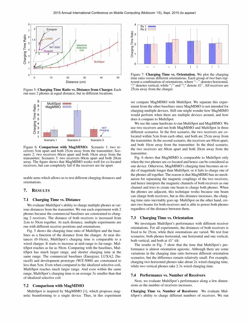
Figure 8: MultiSpot’s Performance with Number of Receivers. (a) MultiSpot’s charging time ratio with up to 6 receivers; (b) MultiSpot’sefficiency as a function of receiver number and distance to the charger. (c) MultiSpot’s maximal charging range increases with receivers.

experiments with 1, 2, 4, and 6 receivers. In each experiment, all ofthe receivers are placed at the same distance from the charger, butat random positions and orientations. To show the results we pickthree representative distances, 2cm (near range), 25cm (mid range)and 50cm (far range). Fig. 8a shows the charging time ratio versusnumber of receivers. In all cases MultiSpot is able to charge all ofthe phones. However, the charging time increases with distance andnumber of receivers. This is because MultiSpot needs to split morebeams when there are more receivers, so the power that is carriedin each beam will go down with more receivers.

Efficiency vs. Number of Receivers: We test MultiSpot’s effi-ciency with different locations and number of receivers. The dis-tance of all receivers to the transmitter is fixed while the numberof receivers is increased. For a given distance and number of re-ceivers, the positions and orientations are varied across runs. Weevaluate MultiSpot’s efficiency. Similar to past work [1], we defineefficiency as the ratio between the total received power at all receiv-ing coils divided by the total input power at the transmitting coils.The experiment is repeated with 3 different distances: near range(2cm), mid range (25cm) and far range (45cm). For each range werepeat the experiments for different number of receivers.

Based on Fig. 8b, we make a few observations:

• For a single device, MultiSpot has similar or better efficiencycompared with state-of-the-art systems. For example, Mag-MIMO [1] reports 89% and 34% efficiency with single deviceat 2cm and 20cm, while MultiSpot’s efficiencies are 90% and38% at 2cm and 20cm, At near range, MultiSpot’s efficiency isbetter than commercial systems. For example, WiTricity WiT-5000 [15] reaches its best efficiency (90%) at 0.6cm, while Mul-tiSpot has 90% efficiency at a larger distance (2cm).• We also find it interesting that the system efficiency increases

with the number of receivers. For example, at 45cm the efficiencyincreases from 14% with single device to 43% with 6 receivers.This effect is more apparent when the receivers are at mid-rangeand far-range. The reason is that the more receivers are around,the more magnetic flux can be picked up by the receivers. Thishappens because the beams are relatively wide, and hence whenthere are more receivers, they can collectively pick up more en-ergy.

Maximal Range vs. Number of Receivers: As the number of re-ceivers increases, the efficiency of MultiSpot increases. With thisincreased efficiency, it may be possible to charge a receiver at alarger distance when more receivers are in the system. Therefore,this experiment is aimed to find the maximum distance from thetransmitter a phone can still charge from, given a number of re-ceivers. To get a feel of how the range increases with number of

12

3

4

5

1:��Tablet

2:��Smartwatch

3:��Wireless�Keyboard

4:��Wireless�Touchpad

5:��Phone

(a) The Experimental Setup

0

1

2

3

Cellphone Tablet Smartwatch Keyboard TouchPad

Charg

ing T

ime R

atio

(b) Charging Time Result

Figure 9: User Experiment: MultiSpot can charge multiple typesof devices concurrently in an office desk scenario as shown in (a).

devices, we put all phones horizontally above the coils and find themaximal z distance. Different phones are aligned and spaced verti-cally.

Fig. 8c shows the maximal charging range vs. the number of re-ceivers. The maximum range does indeed increase with the numberof receivers. From one receiver to two receivers, the distance in-creases by 10cm. With 4 phones, the extension of range is 17cm.

In particular, because of the magnetic coupling between the re-ceivers, one receiver might induce power on another receiver. Inthis case the receiver acts as a power relay, extending the maximalrange of power delivery.

7.5 User ExperimentThe goal of this experiment is two-fold: first, we want to ensure

that MultiSpot works with a diversity of devices; second, we wantto show that MultiSpot could charge all devices while the user isinteracting with them or moving them.

We use the same setup as used by other experiments. However,we involve a variety of receiver devices. Specifically, we have testedcellphones (iPhone 4s/5s/6, Nexus 4, Samsung Galaxy S4/S5, HTCEvo and Motorola Droid X2), tablets (Samsung Glaxy Tab 4 andKindle Paper White), smartwatch (Samsung Gear Live Smart-watch), wireless keyboard (Logitech K810) and wireless touchpad


0

20

40

60

80

100

0 0.5 1 1.5 2

Charg

e (

%)

Normalized Charging Time

Rx 2Rx 1

(a) Same Distance and Initial Battery

0

20

40

60

80

100

0 0.5 1 1.5 2 2.5 3

Cha

rge (

%)


Rx 1Rx 2

(b) Different Distances

0

20

40

60

80

100

0 1 2

Ch

arg

e (

%)


Rx 1Rx 2

(c) Different Initial Battery

Figure 10: Charging Curves of Two Phones For Three Scenarios: The x-axis is charge time normalized by charge time of a wall plug tocharge from dead battery to full. The scenarios are: (a): Charging two phones from dead batteries, with the same distance (25cm); (b): Sameas (a), but with different distances (Rx1: 10cm, Rx2: 40cm). (c): Same as (a) but the two phones start with different battery levels (0%, 50%).

70

75

80

85

90

95

100

0 50 100 150 200

No

rma

lize

d P

ow

er

(%)

Movement Speed (cm/s)

Figure 11: Normalized Power vs. Motion Speed. We plot the nor-malized received power versus different movement speed of the re-ceiver. The reduction of received power is less than 3% when thespeed is less than 50cm/s; it goes up to 20%-30% when the receivermoves at 200m/s.

(Logitech T650). In each experiment, we place the keyboard andtouchpad flatly on the desk, and place the tablet against a stand.We then ask the user to sit in front of the desk and type on the key-board, with a cellphone in her pocket and a smartwatch on her wrist(see Fig. 9a for a photo while the experiment is running). We mea-sure the charging time ratio for each type of devices. We repeat theexperiment with 3 users.

Fig. 9b shows the charging time ratio of the various device types.MultiSpot can charge all of the devices, however the charging timeratio of each of them is different. The cellphone and smartwatchhave relatively higher charging time ratios and standard deviations.This is because they are carried by the user, while the other devicesare static on the desk. Also, according to Fig. 9b, the cellphonetakes longer than the smartwatch to charge. This is because as theuser works, their wrist is moving above the desk while the phoneis in their pocket, so naturally the phone is on average farther awayfrom the coils.

Finally, we have used a temperature gun infrared thermome-ter [43] to monitor the temperature of the devices during the ex-periment. The maximal temperature increase we have measured is4◦C over a duration of 5 hours.

7.6 Power Distribution among ReceiversIn this section, we select three representative scenarios to show

how MultiSpot distributes power among receivers. We charge twoiPhones 5s, in different scenarios:

• Same Distance and Initial Battery: We put each of the twophones 25cm away from the charger and let them charge froma dead battery. Fig. 10a shows their charging curve, i.e., batterypercentage vs. time. Since all factors of these two phones are al-

most exactly the same, the phones charge at the same rate, asshown in the figure.• Different Distances: We charge two phones with dead batter-

ies but with different distances from the transmitter (10cm and40cm). Fig. 10b shows the charging rate of the two phones. Thefigure shows that initially, the phone closer to the transmitter(i.e., Rx1) charges faster since it has a stronger magnetic cou-pling with the charger. However, once this phone is fully charged,MultiSpot transfers the power to the second receiver (Rx2), in-creasing its charging rate. Said differently, when one phone isfully charged and has no demand for power, MultiSpot automati-cally re-allocates the power to serve the other receiver which stillhas demands.• Different Initial Batteries: We repeat the previous experiment,

with different battery levels (0% and 50%). The results presentedin Fig. 10c show that the phone with a lower battery level chargesfaster. Thus, when all other factors are the same, MultiSpot allo-cates more power to the device that has a lower battery level, i.e.,the device with higher demands for power.

7.7 Performance vs. MotionIn this experiment, we aim to evaluate MultiSpot’s performance

with regard to the motion of the receiver. We use the same setupas other experiments, but add controlled movements to the receiver.Specifically, we attach the receiver to a motor which moves acrossthe table where the charger is mounted, and vary the speeds acrossdifferent experiments. During the experiments, the receiver is al-ways 15cm above the table.

To measure MultiSpot’s performance, we pick 5 evenly distancedlocations in the motion’s path, measure the received power at eachlocation, and average them. We then normalize it by the powerwhen there is no motion. Fig. 11 shows the normalized power ver-sus motion speed. We can see that MultiSpot works well with mildreceiver motion, and degrades if the speed increases. Various sur-veys [44, 45, 46] have suggested that the average speed of naturalhuman arm movements is under 50cm/s, in which case the receivedpower is almost unaffected (<3% degradation). If the speed reaches200cm/s, the reduction of power is around 20%-30%.

8. CONCLUSIONThis paper presents MultiSpot, a power hotspot that can charge

multiple devices wirelessly and simultaneously, at distances up to50cm. MultiSpot can be attached to an office desk, and used tocharge surrounding electronic devices. It can also charge devicescarried by the user once she is in the vicinity of a MultiSpot charger.This allows MultiSpot to be used in more practical scenarios, wherethe area of movement by the user is relatively constrained, such as


bed-stands, car seats, coffee shops, airports waiting seats, etc. Webelieve MultiSpot pushes the state-of-the-art of wireless chargingand significantly improves the user experience. Important tasks forfuture work include evaluating our system for a wider range of mo-bile devices and applications, and allowing the system to explicitlyspecify how much power is delivered to each receiver.

9. ACKNOWLEDGEMENTSWe thank the anonymous reviewers and shepherd for their con-

structive comments. We are grateful to Omid Abari, Fadel Adib,Haitham Hassanieh, Swarun Kumar, John MacDonald, Deepak Va-sisht, for their constructive feedbacks. We also thank the NETMITgroup for their support. This research is funded by NSF. We thankmembers of the MIT Wireless Center: Amazon, Cisco, Google, In-tel, Mediatek, Microsoft and Telefonica for their interest and gen-eral support.

APPENDIXA. PROOF OF THEOREM 4.1

Proof: We start with converting the optimization problem to an-other equivalent one. Specifically, if we define ~x =

√RT

~iT , 8 then

the problem becomes that we want to find~ibfT =

√R−1T ~xbf

T , where

~xbfT is the solution to the following:

~xbfT = arg max

~x

{~x∗A~x} , whereA ,√R−1T H

∗RRH√R−1T

The constraint correspondingly becomes ~x∗~x + ~x∗A~x = P .Now, since A is a positive semi-definite Hermitian matrix (recallboth RR and RT are real positive diagonal matrices), it can beeigen-decomposed to A = QΛQ∗, where Q is a unitary matrixand Λ is a diagonal matrix of the eigenvalues of A. Furthermore,all eigenvalues, λ1, · · · , λn, are real and non-negative. If we de-fine ~x′ = Q∗~x, then the objective function ~x∗A~x can be writtenas(~x′)∗

Λ~x′ =∑i λi|x

′i|2. Similarly, the constraint becomes:

~x∗~x + ~x∗A~x =(~x′)∗~x′ +

(~x′)∗

Λ~x′ =∑i(λi + 1)|x′i|2.

Therefore, we have converted our optimization problem to:

max∑i λi|x

′i|2

s.t.∑i(λi + 1)|x′i|2 = P

Since all λi’s are real non-negative, the optimal solution ~x′ is zeroin every entry except the one that λi is maximal. More formally, saythat λk = arg max{λ1, · · · , λn}, then ~x′ is zero on entries exceptthe k-th one. In this case, the maximal value that is achieved isλkλk+1

P . Recall that ~x′ = Q∗~x, or equivalently, ~x = Q~x′. There-fore, the optimal solution ~xbf

T is proportional to k-th column of Q(i.e., the k-th eigenvector of A). Substituting back ~x =

√RT

~iT ,we get the optimal~ibf

T :

~ibfT = c ·

√R−1T ·maxeig

(√R−1T H

∗RRH√R−1T

)In this paper, to simplify the equations, we assume the transmitter

coils are identical, i.e., RT1 = · · · = RTn = RT . In this case,RT is proportional to an identity matrix, thus when multiplied withanother matrix, will not change it eigenvectors. Therefore, in thiscase, the solution is~ibf

T = c · maxeig(H∗RRH). c is a scalar thatcapturesRT and other terms. It can be solved by substituting~iT by~ibfT to the constraint~i

∗TRT

~iT+~i∗TH

∗RRH~iT = P . Note that thisdoes not substantially change any of the conclusions in this paper;plugging backRT into them is straightforward.8√RT is a diagonal matrix whose diagonal entries are square rootof those ofRT . Similarly,

√RR can be defined.

B. PROOF OF THEOREM 4.2Let’s first expand H∗RRH and Y : H∗RRH =

ω2M> (Z−1R

)∗RRZ

−1R M , and Y = ω2M>Z−1

R M .Recall that M is a real matrix, therefore in order to proveH∗RRH = Real(Y ), what we need to prove is(

Z−1R

)∗RRZ

−1R = Real

(Z−1R

)which is proved as follows:

Proof: Note that: 1)RR is the real part of ZR, therefore,

RR =1

2

(ZR +ZR

)(15)

whereZR means entry-wise conjugate ofZR; 2)ZR is symmetric,i.e.,ZR = Z>R , thus by conjugating both sides, we getZR = Z∗R.Inverting both sides yields(

ZR)−1

=(Z−1R

)∗(16)

Substituting them, we get:(Z−1R

)∗RRZ

−1R

Eq. (15)=⇒ 1

2

(Z−1R

)∗ (ZR +ZR

)Z−1R

Eq. (16)=⇒ 1

2

(Z−1R

)∗+ 1

2

(ZR)−1

ZRZ−1R

Eq. (16)=⇒ 1

2

(Z−1R +Z−1

R

)= Real

(Z−1R

)Thus,

(Z−1R

)∗RRZ

−1R = Real

(Z−1R

).

C. PROOF OF THEOREM 4.3We prove the theorem by showing that the rank of Y − Y gets

reduced in every iteration, by the following lemma:

LEMMA C.1. For any complex symmetric matrix A (i.e., A =

A>), any vector ~η such that ~η>A~η 6= 0, define ~ξ = A~η, then

rank(A− ~ξ~ξ

>

~ξ>~η

)≤ rank(A)− 1.

Proof: Since A is a complex symmetric matrix, there exists anAutonne-Takagi factorization [47] such that

A = QΛQ>, where Λ =

[Λ0 OO O

]where Q is a n × n unitary matrix, and Λ0 is a r × r diagonalmatrix, where r is the rank of A. Now substitute this as well as~ξ = A~η, we get:

A−~ξ~ξ>

~ξ>~η

= Q

(Λ− ΛQ>~η~η>QΛ

~η>QΛQ>~η

)Q> (17)

Define ~ζ = Q>~η, and substitute it into Eq. (17), we get

A−~ξ~ξ>

~ξ>~η

= Q

Λ0 − Λ0~ζ0~ζ>0 Λ0

~ζ>0 Λ0

~ζ0

~0

~0>

O

Q>Since Q is unitary, the rank of A − ~ξ~ξ

>

~ξ>~η

is equal to the rank of

Λ0 − Λ0~ζ0~ζ>0 Λ0

~ζ>0 Λ0

~ζ0, which we define as matrixB. If we define ~ζ0 to

be the first r entries of ~ζ, we observe that:

B~ζ0 = Λ0~ζ0 −

Λ0~ζ0~ζ>0 Λ0

~ζ>0 Λ0

~ζ0

~ζ0 = Λ0~ζ0 −Λ0

~ζ0 = ~0

i.e., B is not full rank, such that rank(B) ≤ rank(A) − 1. There-

fore, rank(A− ~ξ~ξ

>

~ξ>~η

)≤ rank(A)− 1.


SinceY is a complex symmetric matrix, we can setA = Y −Y ,~η = ~iT , thus ~ξ = (Y − Y )~iT = ∆~vT . Therefore, applying the

lemma, we get: rank(Y − Y − ∆~vT ∆~v>T

∆~v>T~iT

)≤ rank(Y − Y )− 1.

This means that the rank of Y − Y gets reduced by at least 1 ineach iteration. Since the initial rank cannot be larger than n, whichis the size of the matrix, then the number of iterations that is neededcannot exceed n.

D. PRE-CALIBRATIONThe goal of pre-calibration is to estimate ZT . It can be done im-

mediately after manufacturing the transmitter coils where their rel-ative positions are hardcoded. During pre-calibration, there is no re-ceiver around, so the Transmitter Eq. (6) is reduced to ~vT = ZT~iT .Now, in order to estimate ZT , we need to apply n different sets of~vT and measure the corresponding ~iT . ZT can be consequentlyobtained by matrix inversion, i.e., similar to how we estimate Y inSec. §4.2.

10. REFERENCES

[1] J. Jadidian and D. Katabi. Magnetic MIMO: How to chargeyour phone in your pocket. In ACM MobiCom, 2014.

[2] A. Sample, B. Waters, S. Wisdom, and J. Smith. Enablingseamless wireless power delivery in dynamic environments.Proceedings of the IEEE, 101(6), 2013.

[3] Datasheet for Qi-enabled charger. RAV Power.[4] Duracell powermat for 2 devices. Duracell Corp.[5] Energizer dual inductive charger. Energizer.[6] Qi specification 1.1.2, 2014. Wireless Power Consortium.[7] Rezence specification. Alliance for Wireless Power.[8] Highly resonant wireless power transfer: Safe, efficient, and

over distance. Technical report, WiTricity Corp, 2012.[9] Wattup. Energous Corp.

[10] Cota wireless power. Ossia Inc.[11] Wireless charging, at a distance, moves forward for ubeam,

2014. The New York Times.[12] Wi-charge. http://www.wi-charge.com/about.php.[13] F. C. Delori, R. H. Webb, and D. H. Sliney. Maximum

permissible exposures for ocular safety (ansi 2000), withemphasis on ophthalmic devices. 2007.

[14] M. Zahn. Electromagnetic Field Theory: A Problem SolvingApproach. Krieger Pub Co, 2003.

[15] WiT-5000 development kit data sheet. WiTricity Corporation.[16] TX-200 dual wireless charging pad. LUXA2.[17] Nokia wireless charging plate. Nokia Corp.[18] J. Cassell. http://press.ihs.com/press-release/technology/appl

e-watch-spurs-rapid-growth-market-wireless-charging-wearable-technology.

[19] P. Li and R. Bashirullah. A wireless power interface forrechargeable battery operated medical implants. Circuits andSystems II, IEEE Transactions on, 2007.

[20] S. Kim, J. S. Ho, and A. S. Poon. Wireless power transfer tominiature implants: Transmitter optimization. Antennas andPropagation, IEEE Transactions on, 2012.

[21] U. K. Madawala and D. J. Thrimawithana. A bidirectionalinductive power interface for electric vehicles in V2Gsystems. Industrial Electronics, IEEE Transactions on, 2011.

[22] B. Tong, Z. Li, G. Wang, and W. Zhang. How wireless powercharging technology affects sensor network deployment androuting. In Distributed Computing Systems, IEEE, 2010.

[23] L. Xie, Y. Shi, Y. T. Hou, and A. Lou. Wireless powertransfer and applications to sensor networks. WirelessCommunications, IEEE, 2013.

[24] Proxi-point transmitter for the LTC4120. PowerByProxi.[25] A. Kurs, A. Karalis, R. Moffatt, J. D. Joannopoulos,

P. Fisher, and M. Soljacic. Wireless power transfer viastrongly coupled magnetic resonances. 317(5834), 2007.

[26] B. L. Cannon, J. F. Hoburg, D. D. Stancil, and S. C.Goldstein. Magnetic resonant coupling as a potential meansfor wireless power transfer to multiple small receivers. PowerElectronics, IEEE Transactions on, 2009.

[27] J. Casanova, Z. N. Low, and J. Lin. A loosely coupled planarwireless power system for multiple receivers. IndustrialElectronics, IEEE Transactions on, 56(8), 2009.

[28] J. Kim, D. Kim, and Y. Park. Analysis of capacitiveimpedance matching networks for simultaneous wirelesspower transfer to multiple devices. Industrial Electronics,IEEE Transactions on, 2014.

[29] J.-W. Kim, H.-C. Son, D.-H. Kim, K.-H. Kim, and Y.-J. Park.Analysis of wireless energy transfer to multiple devices usingcmt. In Microwave Conference Proceedings, IEEE, 2010.

[30] D. Ahn and S. Hong. Effect of coupling between multipletransmitters or multiple receivers on wireless power transfer.Industrial Electronics, IEEE Transactions on, 60(7), 2013.

[31] A. Kurs, R. Moffatt, and M. Soljacic. Simultaneousmid-range power transfer to multiple devices. AppliedPhysics Letters, 2010.

[32] D. Ahn and S. Hong. A study on magnetic field repeater inwireless power transfer. Industrial Electronics, IEEETransactions on, 2013.

[33] B. Waters, B. Mahoney, V. Ranganathan, and J. Smith. Powerdelivery and leakage field control using an adaptivephased-array wireless power system. (Accepted andPre-Published) IEEE Transactions on Power Electronics.

[34] M. Moon. uBeam demo video.http://www.engadget.com/2014/08/07/ubeam-wireless-charger-ultrasound/.

[35] S. Budiansky. Truth about Dogs. 2000.[36] Performance standards for microwave and radio frequency

emitting products. Title 21, Part 1030, U.S. Food and DrugAdministration.

[37] W. H. Paul Horowitz. The Art of Electronics. CambridgeUniversity Press, 1989.

[38] Understanding li+ battery operation lessens charging safetyconcerns. Technical Report APP 4169, Maxim IntegratedProducts, Inc., 2008.

[39] Can witricity technology transfer power through walls orobstructions? http://witricity.com/technology/witricity-faqs/.

[40] AD8333: DC to 50 MHz, dual I/Q demodulator and phaseshifter data sheet (Rev. E). Analog Devices.

[41] Zynq-7000 all programmable soc (z-7010, z-7015, andz-7020): Technical reference manual. Xlin.

[42] M. K. Kazimierczuk. Class d voltage-switching mosfetpower amplifier. In Electric Power Applications, IEEE, 1991.

[43] Temperature gun infrared thermometers. Omega Inc.[44] P. Morasso. Spatial control of arm movements. Experimental

Brain Research, 42(2), 1981.[45] C. Atkeson and J. Hollerbach. Kinematic features of

unrestrained vertical arm movements. The Journal ofNeuroscience, 5(9), 1985.

[46] W. Abend, E. Bizzi, and P. Morasso. Human arm trajectoryformation. Brain, 1982.

[47] T. Takagi. On an algebraic problem related to an analytictheorem of Carathéodory and Fejér and on an allied theoremof landau. Japan. J. Math, 1, 1924.


wireless power hotspot that charges all of your · pdf filewireless power hotspot that charges...

Documents