Annales Academic Scientiarum Fennicre

Series A. I. MathematicaVolumen 7, 1982, 279-290

ON QUASI.PARABOLIC PROBLEMSWITH NORMAL BOUI{DARY COI{DITIOI{S

VEIKKO T. PURMONEN

Introduction

In the present paper we study initial-boundary value problems of the form

A(010t, D*)u - f0o ulWl,-o: Qx

in R* X Rn*,

on Ri,

Bi(010t, D)u\,,=o: gi on R+ XR'-1,

where A(010t, D*) and B j(010t, D,) are linear partial differential operators withconstant complex coefficients or, briefly, differential operators in R,XR}. Theproblems considered are quasi-parabolic in the sense defined in [2] and their lateralboundary operator system {Bi@lilt,D,)} is normal to the hyperplane xn:O.

In our previous work [2] we gave a necessary and sufficient condition for prob-lems of quasi-parabolic type to have solutions in a setting of certain anisotropicSobolev-type spaces. We also proved a necessary and sufficient condition for the valid-ity of an a priori estimate between a solution and the data. The aim of this paper is

to show that the general conditions mentioned above will take very concrete formsin the case under consideration. The special case in which thelateralboundaryoper-ators are of the form B1:B.(D,) was already discussed for illustration in [2]. Thegeneral case is, however, more difficult and requires a different treatment.

We state our main results, Theorem 2.3 on the solvability and Theorem 2.4 onthe a priori estimate, in Section 2 after the preliminary first section; in order to avoidoverlapping in introducing the necessary notions we shall refer to [2]. The proofs ofthe main results make essential use of some propositions concerning weighted an-

isotropic Sobolev spaces and of a trace result; which are given in Sections 3 and 4,respectively. In Section 5 we prove Theorem 2.3, and the proof of Theorem 2.4 isfinally given in Section 6. Note that throughout the paper the symbol C is used todenote a generic positive constant.

It seems to us that some more or less loose ideas of compatibility appearing inconsiderations of initial-boundary value problems can be made precise by the meth-ods of [2] and this work.

280 Vrrxro T. PUnMoNEN

1. Preliminaries

1.1. We begin with some notation. We set

(*, t) : xr**...*xn(nfor x:(x', xn):(x1, ...> xn-ls x,)€Ro:R! and €:((r,..., 6r)€ft'. Let

R! : {x : (/, x)€Nlx, = 0},

Q: R* XR! cRrXRl,

^E : R+ XR'-lcnrxRl;l,

whereR+:Rr,*:{r6R,lr>0}.

For every multiindex d.:(ar,...,a,)(N' we write

1*: ti,...€? and Dn : D1,...D7

with p-p"-(D1,...,Dn), D*:-i0l0x* (i:l-a|, in addition, set 0r:010t.By y, and y, we denote the trace operators with respect to I and x,, respectively.

1..2. Let nto,rrh,...,mn be positive integers, F:max{my}, q1,:Ulmo, and

Q:(qr, ...,8,).We shall consider differential operators

A(il, D) : oro*/*n =rah,ilD

(k€N, s€N')

andBi(\r, D) : - Z. bi*o\fD, i : 1,..., %,

kqo+<d,q)=pi

where aoo and by,o are complex constants, ,tr.;>0 is the order of Bi(\r, D), andx=ffio is a positive integer. We can and shall write them in a self-explanatory manner

also in the formA(D,,D): Z Ak(D)\f,

k=mo

Bi(O,, D) : on7=r,Bt*(D)01;

note that we prefer here to write for example Ay(D) instead of A@ (D) used in [2].

1.3. Problem (QP). We shall study the initial-boundary value problem

A(0,, D)u : f in Q,

yriltu : Er, on Rl , k : 0, ..., ffio-|,

YnBi(\t, D\u : gi on », i : l, "', x;

as in [2] we call it Problem (8P).

On quasi-parabolic problems with normal boundary conditions 28t

In the realizations of Problem (QP) the dxa f,9*, g j, and the solution z willlie in certain function spaces of the Sobolev type.

1.4. Basic spaces. The norm of a (complex) normed space X is denoted by

ll . llx. If X,Y, and Z are three normed spaces with XcZ and YcZ algebraically

and topologically, let XaY be equipped with the norm

ll ull x nv : (ll ulli^ + ll ull?)t t'z.

Let s>0 and let Xbe a Hilbert space. Assign the weights qo and 4p to differen-

tiation with respect to / and x1, respectively. Then we can introduce in a usual way

the Sobolev-type space H"(Q;X) of X-valued distributions d)*X, used here foro:R or R.., and further the anisotropic spaces H"(a) with g:Ri or Ro-l,and F1(")1o;:H","(Q),äf)(o), ana a[å]1o; with Q:Q or .E. For the definitions

of these spaces we refer to [2] and to the references given there.

The weighted Sobolev space ä"(R +i a; X) with the weight function e-a',g>0, is defined to consist of the distributions u: R*tf, with e-a'u(H"(R*;X)and is equipped with the norm

ll nllrr'rn* ;e;xl : lle-a'ullru"G *:x)'Finally, define

H@(Q; c) : ä"(R+; s; rr.(Ri)) n I/.(R*; a; ä"(R'l))

and analogously ä(")(^»; g) as well as the spaces nP@;q) and a$l«o; e) withg:Q or X. See [2].

2. Main results

Suppose that the operators A(At, D) and Bi(|r, D), i:1, ...) 2,c, are given as in

1.2, and set for brevity

^ l.ö : ;(qo_r

q")

andÅ(p.i) : {s€Rls > mar( tu}+q"lZ},

R(p, p): {s6Å(p;)ls = r},

Rqo(p, pi) : {s(RQr, p)ls * qol2mod qo}'

Without further mention, we assume S=0.We make the following hypotheses:

Hypothesis l. Problem (8P) is quasi-parabolic, i.e., the operator §ystem

(A (ot, D), (y,ilt)tr:o', (y, B i(0,, o))i =r)

is quasi-parabolic in the sense defined in l2l.

282 Vurro T. PUnMoNEN

Remar,k. We can and shall assume that the coefficient d.o,o is equal to one.

Hypothesis 2. The operator system

Bt(il,D), ..., B*(il,D)is normal to E:

(i) Bj(Oo D) is normal to 2 of order pJ, j:1, ...,x, that is, qnl7i and the coef-

ficient of Dfile" differs from zero;(ii) pi#p1, for j#k.2.1. Initial and boundary values. Let r€R(p, pj). Suppose

ueV@(Q;g) and set

f : A(0,, D)u,

Qr,: Tr0l u, k : 0, ..., n1o-1,

gi : T,Bi(0,, D)u, i : l, ..., x.

Then, firstly, the initial values

ils: y,O!u, O = kqo= s-qol2,

satisfy (see [2], Theorem 7.2)

(1) 0*: ex, k : O, ..., nto-L,

e) e^o*, : T,f+^§ ,s"-, -:f ' A*(D)En*x, 0 = rqo < s- tt- Qol2.y:0 &:O

Here the operators ^§, and T, arc defined by

§-r: O r:1,2r...,So : -Id (Id : identity),

s, :-,§ Ak(D)s,-^.+k, r : r,2,,..,t:o

andT-r:0, r:1r2r.,.,

mo-LT,: .lrfli- Ä Ak@)f,_mo+k, ," : 0, 1, ....

Secondly, the initial values @,, and the boundary values g; satisfy the conditions(LCR) and (GCR):

(LCR) If pi*vqo<s-6 with tQN, then

Y,\'lgi: Y,. Z By(D)iD"+*.kqo=ul

On quasi-parabolic problems with normal boundary conditions 283

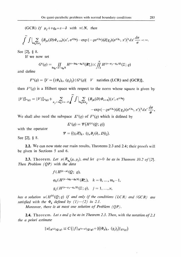
(GCR) If pi*vqs:s-ö with Y€N, then

F n, <ra-\ \, cr^ ,,,- . ,do

of Ilrr?=-,(Bik(D)o"*k\(x',o"tao)-gxp(-s6slr")(0ig)(o'to",x)l'dx':::-<@.

See [2], § 8.

If we now set

G"(q) : II gs-wo-aot2(R\)X n HG-t'i-s^tz)(». e)kao<s-qo/2 i:rand define

F"(8) : {v : ((Ö)o, (gr)) e c'(e)l I/ satisfies (LCR) and (GCR},

then F"(g) is a Hilbert space with respect to the norm whose square is given by

ll Z ll ?.<nr : ll r/ll ä"(q) + r, *,2*

" - o i I I r,å r,(B ik(D) o

" + k) (x', o" r'01

-exp (- go" tsi(Ai g )@"/a,, x'112 dx' !9.We shall also need the subspace .8"(q) of F"(q) which is defined by

ä"(8): V(tt<"t17' n1with the operator

V : ((y,01)r,, (y"Bj(\t,D))).See [2], § 8.

2.2. We can now state our main results, Theorems 2.3 and 2.4; their proofs willbe given in Sections 5 and 6.

2.3. Theorem. Let s€Rno(&, p), and let q>O be as in Theorem 10.2 of l2l.Then Problem (QP) with the data

f€u<"-rt19' n..'

g*CHG-tqo-eolz) (R"a), k:0, ..., tno_!,

gi€H("-t'i-a"t»(E; Q), i : !,.-.,%,

has a solution u€H@(Q;d if and only if the conditions (LCR) and (GCR) aresatisfied with the iDo defined by (1)-(2) in 2.1.

Moreouer, there is at most one solution of Problem (QP).

2.4. Theorem. Let s and p be as in Theorem 2.3. Then, with tlrc notation of 2.1the a priori estimate

ll zllB<'r,n,n, = C(ll/lla«"- *r(etd*ll((@Jo, (gr)Jllr"rnr)

284 Vrrxro T. PUnMoNEN

of,

it

holds for atl u(H@(Q;e).

Remark. The reversed estimates are valid, too. Note also that the right sides

of the estimates virtually depend only on .f,(E)r, and (gi);.

3. Some basic results on ä$]-spaces

For the proofs of the main results we shall need the following three propositions.Their proofs will be only briefly sketched.

3.1. Proposition. Let s>0. Then

u8(Q; s) : I/o(&", + ; r18(r; s)) n ä"(R,, , *; H(o) (z; d)

with equiualent norms.

Proof. We have

Lemma. If s:kq, with ft(N, then the spaces n[i\127 ana

Ilo(R",, * ; Iz,lJ(z)) n i7"(&", + ; ä(o)(r))are isomorphic.

In fact, by definition

n[;] fO: är"(&, * ; ä.(Ri)) n Ho(&,* ; ä"(Ri)).

Now use the extension operator and the Fourier transformation with respect to Ito show, by Fubini's theorem, that the spaces

Hto"(R,,*; äo(Ri))and

Ho (R,^, + ; Htq, (Rr,* ; äo (R' -t)))

are isomorphic. On the other hand, use the extension operator and the Fourier trans-formation with respect to x, to see that the spaces

äo(&, *; ä"(Ri))

equiualently (see l2l, 12.3),

"(o-g-Lo'ulln«><a.o = C[il,filirt"- D(e;p)* Zo llVollo"-kso-solz(Rn+)+ )llSill"a-ri-,tn/z)e;o)

+ Z f flZ@jk@)on+k)(x',o"tq»li+!4o:§-ä{ "'kqo=li -

-exp (- ao'/s1@i C)(on'., {l'al #)

On quasi-parabolic problems with normal boundary conditions 285

andl?o(&,, + i ä0(R,, * i 11"(R'-'))) n H"(n,", *i Ho(R,,+; ä"0(R"-1)

are isomorphic. Then the assertion follows.The result of this lemma can be extended by interpolation to all sE0. To

complete the proof, apply then the mapping u*e-a'tt.

3.2. Proposition. Let Q stand for Q or Z. If sr>sr=Q and sr:(l -0)r.+0s, with 0=0<1, then

täldi)(o; e), ä8) (a; d1': ä8)(o; s)

v,ith equiaalent norms; here lX, Yls denotes the interpolation space for the interpolationcouple {X,Y}of two Hilbert spaces X andY (seelll,Chap. I).

Proof. Since (see [2], Proposition 4.9)

[ä8)(o), fl8)(o)]u : fl8)(o),it suffices to apply the isomorphism

ä8(rz; e) * ä8 (Q):u- e-etu.

3.3. Proposition. Let Q be as in Proposition 3.2, and let s>0,rhen heHfu](o; d if and only if

(i) he Hoat (A; p1

and

(ii) [ I U.n ? so)([ih)(o, y)lzdy!9 =,* if s- qsl2 : vq, with v(N.

Condition (i) is equiualent to the condition

(i') h€H(§)(o; q) and yr\ih:o for o<vqr-s-Qol2,

and (ii) to the condition

(i0 rLtz\ihagtol(O; o).

Furthermore, if s:vqn*qol2 with v€N, then the square of the norm of hcnft)r(O; q)

is eEioalent to

ll hll211 «', 1s, 6 * ll t - L/ 2

0n hll211 a4s. e1 .

Proof. In order to prove the first part, it is essentially enough to note that

x: e-ath(fl69(o)if and only if xe ä[")(lZ) and

f 1 fU r><r, v)l'dv L - * if s : rqs* qsf 2,

and then to employ the Leibniz formula.

286 VErrro T. PUnMoNEN

To verify the equivalence of the norms, observe first that the square of the normof hen$l(a; s) is equivalent to

lle-n'hllL"(*., po1*lle-" hll217os1*; u.)yllt-ttz 0i@-e' h)llzro1**,17o1,

where ä" stands for E(R"*) or ä'(R'-1), F:0, s. Next show that

llt -r/2 e- at 0f hllso6* ; aol < C llhll u«» p ; et

for k<v, and use the Leibniz formula to obtain

llhllL $1ro, nt = c ( ll å ll i, <. r 6, 6 * ll t-' /' 0i hlll1,, » p. ).

The reversed estimate follows from the inequality

11t-'/' 0i h11 rro)(o; a) E C ll åll7r15;1o; qy,

proved by induction, for example.

4. Ä trace result

4.1. Proposition. Let s€R(pi). Suppose Hypothesis 2 is satisfied. Then themapping

(T,Bi(0,, o)),:n[;l(Q; d * II Hffyu-e"tzt7»' p1

is a continuous surjectiae operator which has a conlinuous linear right inuerse Bjt"

Proof. First we have

Lemma. The mapping

(y,Di) i q^., - t"1 r: H [ål (Q' d * { H lål i s" - s"t 2) (» : Q)

is a continuous surjectiue operator with s continuous linear right inuerse (y)^t.

To see this, use a known trace result (see [1], § 4.2), Propositions 3.1 and 3.2,and the open mapping theorem.

From the previous lemma and from Proposition 6.7.4 of l2l it now follows in theusual way (cf. [3], Section 7-8) that the assertion is true for any Dirichlet system

Fk(\t, D), 0 < keo < s- qnl2,

where the order of Fk(A» D) is kqn and the coefficient of Dl differs from zero. LetF*1 denote the corresponding inverse.

Finally, to prove the general case, it suffices to extend the system {Bi(On D)lto a Dirichlet system {Fo(|r, D)} and then to consider an appropriate restriction of

__lthe lnverse ,8R'.

On quasi-parabolic problems with normal boundary conditions 287

5. Proof of the solvability (Theorem 2.3)

5.1. We first recall the following general result:

Theorem. ([2], Theorem 11.2.) Let s€Rqo(F, F), and let g be as in Theorem10.2 of l2l. {Inder Hypothesis I Problem (QP)-has a solution u€H@79; g if andonly if

((oo)0, (gj»)€ä"(s).

Moreouer, there is at most one solution.

Thus we are led to prove the next theorem.

5.2. Theorem. Let s€rR(p;). Under Hypothesis 2 we haoe E"(S):F"(q).

Proof. Let V:((iD)*, (g;»)e r"(e). First define

u : (yi)n.(@)o€H@(e; q),

where (7)a1 is the continuous linear right inverse of the operator

yi: (yr0t)rno<"-qoniH@)(Q; d * f! Hs-wo-aot'(R"*);

see [2], Proposition 4.7. Set now

and fi : ynBi(\r, D)u(lf{"-at-utzt(E; q')

Then hi: Ei-fi.

((@)x,U)): Yu(E"(Q\,so that

((0)k, (t j)j)€r"(s).Thus we have

and "!t\ih, :0 if Fi*vqo < s-ä

! I p*nt- po)(Dihi)@, x)lzdx' !9

=* if ttitvqo: s-ä.

Hence rrjo.itior, 3.3 implies that

hrcU[61r't-t"tz)(E; e), i : l, .-., x.

If we set, applying Proposition 4.1,

then w: Bl'(h)ieä8(0's),

ynBi(\r,D)w: hi, j :1, ...,x,

288 Vrrrro T. PUnMoNEN

and, by Proposition 3.3,

lr\fw - 0 for Q = kqo< s-8012.

Let us now define

Then Lt - u *w€Fl(') (e; d.

!r\fu - Qo, 0 = kqo< s - 8012,

and

TnBi(O,, D)u - fj*h, : Ej, i : t, ..., %,

that is,((o)0, (g;)i) - vu€E'(q).

Thus we have F'(e) cB'(e), and consequently E'(e) : F' (e).

6. Proof of the a priori estimate (Theorem 2.4)

6.1. We can make use of the next theorem.Theorem. ([2], Theorem 12.2) Let s€Rao(Ir, F), and let g>0 be as in Theorem

10.2 of l2\. Under Hypothesis I the a priori estimate

ll ull u< "t <a. o = C (ll f ll rr" -,r 1p, n; * Il ((@Jo, (gi)) ll r. tr)

holds for all uqH@ (Q; d if and only if the operator

V:HG)(e; s) r E"(e)

has a continuous linear right inuerse.

Accordingly, it suffices to prove the following result:

6.2. Theorem. Let s€R(p;). If Hypothesis 2 is satisfied, the operator

y:HG)(e; e) - E"(s)

has a continuous linear right inuerse.

Proof. We employ the proof of Theorem 5.2, and define a mapping

Y;1:8"(q) * H@(Q' O)

by setting, for every V:((<Dr)*, (s);)ef"1q;,

Y*LV : u: u*w: (?i)"t(OJk+BRl(h)j

: (yi[' (@J o + B ;L (g 1 - t, B i (0,, r) (?i )"-' (@k)J, .

Then Ylt is a linear right inverse of V.

On quasi-parabolic problems with normal boundary conditions ZBg

In order to verify the continuity of !{a-1, we first write

yv 1, tt 11 r,., 1e ; d € ll (yi)r t (oo)oll a<,r(o ; n) + IIBR, (åj)i ll.r,,,is. n, .

Here we have (see [2], Proposition 4.7)

ll (7:)R t (ok)rll s(") 10 ; e) = Z ll @r lla, - rcqo- 4t z 1p\1 t

and Proposition 4.1 implies that

11 a;1 (h,),it., t") (o ; e) s C ä ll ä, ll,

15; r 7 - ent z) q2, n1

t

It follows from Proposition 3.3 that

Z llh 1ll'u 16y r, - a.t z) s ; e)

-, (J ll s i - rtll?a - u i - q, (z : r, + r, * ulo:

" _ u

il t -'/' 0i {s i - -fi)lll *, o, n)

: C(Zr*Z).

Using the definition of the -fi, we obtain here

»t = c (1lls,ll|,16yr,-n, tz) p;p1+ I llooll'r"-*to-aorz6\1).

In the sum .X, we have

y,-''' oi ki - rt)lL *, e,, nt

=* "([ ltrnZr@n{o)<D,*o)({,o§l40)-exp 7- qo"tc^)(oi Bi)(o"tq^, x')lzdx' !!

* ul I lrr\_r,(Bit"(D)il"*o)(1, o"rno1-exp (- sos/o'; (0i f)(o"u,, {l' a*' !9).

Since ((Oo)0, (f)):YueE"(q), this gives

» z = C QIV ll?,rnr * ll u ll ä,,,(o ; e)) = C llv llrr" <nt.Thus we have

llY ;t V ll ro rn, 4 = C llV ll r" rn,

for all V(E"(d, which completes the proof.

Remark. Note that the existence of a continuous linear right inverse can alsobe deduced by Theorem 5.2 and the open mapping theorem.

290 Vrrrro T. PunnoNrN: On quasi-parabolic problems with normal boundary conditions

References

[l] LroNs, J. L., and E. MecsNBs: Non-homogeneous boundary value problems and applications.

Volume I. - Die Grundlehren der mathematischen Wissenschaften 181. Springer-

Verlag, Berlin-Heidelberg-New Y ork, 1972.

[2] PunIr,ror.lrN, V. T.: Quasi-parabolic initial-boundary value problems. - Ann. Acad. Sci. Fenn'

Ser. A I Math' 6, 1981, 29-62.[3] Scnrcnrrn, M,: Modern methods in partial differential equations. - McGraw-Hill lnc,,

1977.

University of JyväskyläDepartment of MathematicsSeminaarinkatu 15

SF-40100 Jyväskylä 10

Finland

Received 24 March t982