word count: 5,578 words (excluding tables and figures) + 4 ... · 1 word count: 5,578 words...

Working Paper 1

Word count: 5,578 words (Excluding Tables and Figures) + 4 Tables + 2 Figures = 7,078 words 1

2

3

How Much Has High-Speed Rail Contributed to Economic Productivity in Japan? 4

5

6

Takuma Cho 7

Department of Civil Engineering, The University of Tokyo 8

7-3-1, Hongo, Bunkyo-ku, Tokyo 113-8656, Japan 9

Phone: +81-3-5841-7451; Fax: +81-3-5841-7496 10

E-mail: [email protected] 11

12

Hironori Kato (Corresponding author) 13



Phone: +81-3-5841-7451; Fax: +81-3-5841-7496 16


18

Jetpan Wetwitoo 19



Phone: +81-3-5841-7451; Fax: +81-3-5841-7496 22


24

25

26

Working Paper 2

ABSTRACT 1

2

This study investigates empirically the impact of high-speed rail (HSR) on regional economic productivity in the case of 3

Japanese HSR, which has the longest history of HSR operation in the world. Empirical analyses with an econometric 4

approach are carried out using panel data for 1981, 1986, 1991, 1996, 2001, and 2006, covering 46 prefectures in Japan. To 5

represent regional accessibility, a gravity-model-based accessibility is formulated using the minimum travel times from 6

origins to destinations covering multiple transportation modes. Three econometric models—a pooled model, a fixed-effect 7

model, and a random-effect model—are then employed to estimate impacts on regional economic productivity, using 8

accessibility as well as sociodemographic and socioeconomic factors as explanatory variables. Accessibility is also treated 9

as an instrumental variable, because reverse causation may be expected. The results show that while accessibility has a 10

significant and positive impact on regional productivity, the reverse causal relationship could also be suggested. The 11

findings also show that the presence of HSR stations significantly influences regional productivity and that its impact has 12

been increasing gradually, possibly owing to the historical pattern of agglomeration near HSR stations. The impact of HSR 13

on economic productivity is higher in regions with HSR stations, particularly those located far from the largest cities rather 14

than those neighboring the largest cities. The results could imply that HSR contributes to narrowing the productivity gap 15

between peripheral and urban areas, which justifies HSR projects as a means of regional development. 16

17

Keywords. high-speed rail, economic productivity, accessibility, transportation panel data, Japan 18

Working Paper 3

INTRODUCTION 1

2

Transportation investment is expected to enhance economic productivity and economic growth (1). Many previous studies 3

have shown a positive relationship between transportation infrastructure and economic efficiency. Canning (2) examined 4

the impact of infrastructure stocks over 1950–1995 in various countries around the world and concluded that infrastructure 5

stock including transportation infrastructure has a strong positive relationship with other development factors such as 6

population, urbanization level, and GDP per capita. The World Bank (3) also provided cross-sectional data in 1990, 7

showing that the amount of infrastructure stock per capita tends to be higher in countries with higher GDP per capita. Thus, 8

GDP growth is typically treated as one of the performance indicators of transportation infrastructure development, along 9

with the growth of vehicle distance travel, oil usage, and other transportation data, as shown in Litman (4). In terms of 10

economic productivity gains, improvement in transportation accessibility could, in the short run, directly affect industrial 11

productivity through its impact on factors such as commercial delivery, business travel, and commuting to work and 12

school. In the long run, it could also enlarge market areas, increase potential competitiveness, and change land-use patterns 13

and labor markets, all of which may indirectly affect economic productivity. Banister and Thurstain-Goodwin (5) 14

suggested that transportation investment affects the local economy at three levels: output and productivity at the macro 15

level, agglomeration economies and labor market effects at the meso level, and land and property market effects at the 16

micro level. Lakshmanan (6) gave a broader viewpoint of the economic consequences of transportation, including gains 17

from trade, technology diffusion, coordination resulting from the “Big Push” effect, and gains from agglomeration. In 18

particular, agglomeration economies have been highlighted recently by many studies such as Graham (7). Chatman and 19

Noland (8) conducted a detailed literature review concerning the agglomeration impacts of transportation investment and 20

concluded that public transportation improvements are capable of bringing substantial external benefits by enabling 21

economies of agglomeration. Deng (9) pointed out that both positive and negative impacts have been reported from past 22

studies and presented potential factors affecting the impacts of transportation infrastructure on economic productivity and 23

economic growth. He also suggested that the contribution of transportation investment to productivity should be carefully 24

examined, taking account of local and market contexts. Summarizing these studies, it appears that economic impacts from 25

transportation development arise from premiums in accessibility and transportation costs, which could further expand 26

economic productivity and economic growth, but this needs to be verified carefully through contextual empirical analysis. 27

Such economic impacts from transportation development, including investments in HSR, have been strongly 28

anticipated by policy makers. HSR is typically assumed to shorten travel times significantly, which could improve 29

accessibility and contribute to regional economic development. To verify the impacts from HSR, however, the following 30

issues that are specific to HSR should be highlighted. First, HSR connects one region with another region; thus, its impacts 31

on productivity are experienced across regions rather than within a region. Thus, inter-regional analysis is required to 32

identify its widespread impact. Second, the economic impacts from HSR should be carefully observed in a historical 33

perspective rather than with a cross-sectional approach, since they could involve long-term rather than short-term 34

processes. Third, HSR typically faces tough market competition from alternative transportation modes; thus, multiple 35

travel modes should be incorporated into the analysis, such as air transportation (10, 11, 12) and expressway travel (13, 14). 36

Fourth, access and/or egress travel to and from HSR stations should be taken into consideration, because the level of 37

service of a last-mile trip could significantly affect the utility of HSR services. This study analyzes empirically the impacts 38

of HSR on economic productivity in Japan. As the Japanese HSR system has the longest history of HSR operation in the 39

world, it can be expected to provide the best available historical data to reveal the long-run economic effects of HSR. It 40

should be noted that six HSR lines and two sub-HSR lines have been gradually introduced into Japan since the first HSR 41

line started operating in the 1960s. This study collects data from 1981 to 2006 regarding regional economic productivity, 42

along with data on HSR services and other competitive transportation modes in 46 prefectures in Japan. The access/egress 43

details of local transportation to and from HSR stations are incorporated into the inter-regional transportation service data. 44

The paper is organized as follows: the next section reviews the existing literature on the economic impacts of HSR. 45

The dataset used for an empirical analysis is then presented. The results of empirical analysis are shown and the findings 46

Working Paper 4

are discussed. Finally, the paper concludes with further analysis and suggestions for future research. 1

2

3

LITERATURE REVIEW 4

5

A number of studies have addressed the impact of HSR from various viewpoints. de Rus (15) suggested that the 6

introduction of HSR generates direct benefit from travel time saving, which increases economic productivity in the short 7

run; while, in the long run, it attracts new activities, resulting in market expansion and increased firm productivity. Chen et 8

al. (16) empirically examined the impact of HSR in a Spanish case using a structural equation modeling approach, 9

concluding that investment in HSR had positive impacts on growth in provincial economies, stimulating GDP and 10

increasing employment levels, leading to wider economic impacts. Case studies of the French TGV system also reported 11

significant development in real estate and large business in Le Mans, Vendôme (17), and Nantes (18). Masson and Petiot 12

(19) provided evidence to support its positive effect on tourism; for instance, data from the TGV southeast line showed 13

growth in hotel visits as well as in the number of conferences held, although HSR also penalized tourism through shorter 14

periods of stay. On the other hand, Chen et al. (20) reported that the introduction of HSR widened the economic gap in the 15

Manchester sub-region, first because the regional economy had been already restructured by other transportation modes 16

and second because intra-regional transportation connecting with HSR was not sufficient. Shen et al. (13) found that cities 17

will receive minimal benefits from HSR if the station is located away from the city center and that the speed of land use 18

development depends on the attractiveness of new HSR stations. 19

More specific to the Japanese HSR system, Nakamura and Ueda (21) compared population growth in regions with 20

HSR stations with those without HSR stations, concluding that the presence of HSR stations is the most important factor 21

for population growth, with accessibility to expressway networks also supporting such growth. Amano and Nakagawa (22) 22

showed that HSR induced more urban redevelopment in the vicinity of new HSR stations located in peripheral regions 23

than did existing HSR stations located in urbanized regions. Based on empirical investigation, Han et al. (14) claimed that 24

access time to Japanese HSR stations plays an important role in affecting industrial location, although the elasticity is 25

smaller than for industrial interdependence and people’s consumption demand. 26

27

28

THE HIGH-SPEED RAIL NETWORK IN JAPAN 29

30

A huge population is squeezed into a very small extent of habitable land in Japan, creating high-density cities along plains 31

and shorelines. This is one of the most important factors that has shaped Japan into a rail-oriented society (23). To serve the 32

huge travel demand between the three largest cities in the middle part of Japan, the Japanese HSR system, called the 33

Shinkansen in Japanese, initially started operation in 1964, connecting Tokyo, Osaka, and Nagoya. The first HSR in the 34

world, the Tokaido Shinkansen, was constructed mainly because the conventional lines connecting these cities had almost 35

reached their full capacity owing to increasing demand brought about by rapid economic growth. The success of the first 36

Japanese HSR encouraged the Comprehensive National Development Plan to incorporate further HSR construction as a 37

means of encouraging regional development. A new line between Osaka and Okayama started to operate as part of the 38

Sanyo Shinkansen in 1972 and was completed in 1975 by the extension to Hakata, the economic center of Kyushu region. 39

The next HSR lines opened in 1982, with the Tohoku Shinkansen between Omiya and Morioka in northern Japan and the 40

Joetsu Shinkansen between Omiya and Niigata. These two lines reached Tokyo prefecture in 1984 and connected with 41

Tokyo station in 1991. Note that contrary to the Tokaido and Sanyo lines, which were constructed to meet the increasing 42

travel demand among large cities located in the Pacific coastal belt, later HSRs such as the Tohoku and the Joetsus were 43

constructed mainly as regional development projects. 44

After the privatization of Japan National Railways into Japan Railways in 1987, new type of HSR called “mini-45

Shinkansen” started operating between Fukushima and Yamagata in 1992. Unlike HSR systems in Europe, Japanese HSR 46

Working Paper 5

is characterized by a complete separation between high-speed and conventional services, each with its own infrastructure 1

(15). A new standard gauge was needed to realize high-speed operation, since the narrow gauge (1 067 mm) of the 2

conventional rail network in Japan restricted its physical connection with high-speed services. Mini-Shinkansen, on the 3

other hand, is characterized by the combined operation of HSR lines and conventional lines, achieved by improving the 4

conventional track. A part of the Hokuriku Shinkansen between Takasaki and Nagano and another mini-Shinkansen called 5

the “Akita Shinkansen” between Morioka and Akita came into operation in 1997. The Yamagata Shinkansen was 6

extended to Shinjo in 1999, and the Tohoku Shinkansen was extended to Hachinohe in 2001. A part of the Kyushu 7

Shinkansen between Kagoshima and Yatsushiro opened in 2004 and connected to Hakata in 2011. The Tohoku 8

Shinkansen was also extended to Aomori in 2010. The Japanese HSR network in 2006 is illustrated in Figure 1. 9

10

11

DATASET 12

13

Accessibility 14

The introduction of HSR improves regional accessibility. This study formulates accessibility through the gravity-model 15

approach. This assumes that accessibility between two regions is affected by socioeconomic or sociodemographic regional 16

factors and that it declines as travel time from one region to the other increases. This study assumes that regional 17

population represents the regional factors, based on the existing research (24). Multiple transportation modes are 18

incorporated into the estimation of inter-regional travel time, because other inter-urban travel modes apart from HSR are 19

also expected to influence accessibility. Regional accessibility is then formulated as below: 20

j

mij

jii

T

PPACC

2.min

(1) 21

FIGURE 1 High Speed Rail Network in Japan as of 2006

Working Paper 6

where i and j represent prefectures, iP represents the population in prefecture i , and mijT represents the 1

minimum travel time from prefecture i to prefecture j when transportation mode m is used. 2

3

Dataset 4

Sociodemographic, socioeconomic, and transportation panel data are prepared by prefecture in Japan for 1981, 1986, 1991, 5

1996, 2001, and 2006. The dataset is presented in five-year intervals, because some data are only available every five 6

years. Note that there are 47 prefectures in Japan. As one of them—Okinawa prefecture—consists of many islands located 7

far from the HSR network, it is excluded from our database. The sociodemographic data include prefectural population, 8

prefectural population by gender, prefectural population by age subgroup, and prefectural employees. 9

Next, the socioeconomic data includes the number of offices, the number of employees by industry, gross regional 10

product (GRP) by industry, and net stock of social capital. Industries are categorized into “primary industry,” including 11

agriculture, forestry, and fishery; “secondary industry,” including mining, construction, and manufacturing industries; 12

“tertiary industry,” including electricity, gas, and water, distribution businesses, finance, real estate, transportation, 13

information and service industries, and the government sector. Note that the GRP and net stock of social capital are 14

deflated to 2005 levels. As for “productivity,” this study assumes that labor productivity represents general economic 15

productivity. Labor productivity is calculated as GRP per employee. 16

Finally, the transportation data consist of the minimum travel time between prefectures and the minimum number of 17

transfers to the nearest HSR station in each of the three largest cities: Tokyo, Osaka, and Nagoya. Note that different data 18

for transportation networks and services are prepared for different years based on the service availability by transportation 19

mode in the past. A representative node in each prefecture is assumed where the prefectural capital is located. The 20

transportation modes cover HSR, conventional rail, air, inter-city bus, and private car. In estimating the travel time of 21

public transportation modes, the minimum access/egress travel time of local public transportation services is assumed for 22

access/egress to and from HSR stations or airports, if such services are available. If local public transportation services are 23

not available, private car is assumed for estimating access/egress travel time. For private car, the minimum travel time from 24

a representative node in an origin prefecture to another representative point in a destination prefecture is computed using 25

the road network data for each year. If the road network does not directly connect an island with others, the use of car-ferry 26

services is assumed. The number of transfers to and from HSR stations is collected from past rail timetables. 27

TABLE 1 shows descriptive statistics of the dataset, which contains 276 records compiled from 46 prefectures over 28

six years. First, average productivity is 7.05 million JPY per employee, ranging from 4.62 to 11.61 million JPY. Note that 29

one US dollar was on average equal to 110.2 JPY at 2005 levels. The average productivity has been increasing, while its 30

standard deviation has fluctuated. The standard deviation was higher in 1991, probably because the Japanese economy 31

experienced the asset price bubble, after which economic disparities among regions become larger. It was also higher in 32

2006, possibly because the government of the day introduced deregulation policies following the new approach of 33

liberalism, which led to higher economic disparities among regions. 34

Second, the accessibility has a quite wide range, from 0.11 to 18.61. This has increased gradually from 1981 to 2006, 35

indicating that the transportation network has been developed, which improved regional accessibility. The standard 36

deviation of accessibility has also been increasing, which may imply that accessibility has improved only in specific 37

regions where there was investment in transportation infrastructure. 38

Third, the number of transfers to any of the three largest cities is 0.43 on average and has been generally decreasing. 39

This may imply that the local access/egress public transportation services in the largest cities have been significantly 40

improved in the past decades. This includes the expansion of local public transportation networks in these cities, enabling 41

passengers to travel directly to the nearest HSR station. 42

Fourth, the share of female population in their 30s out of total population is 6.98 percent on average. Ongoing rapid 43

aging and the lower birthrate in Japan have decreased the share of the younger generation in the population, which led to 44

the decline of the share of the female population in their 30s from 1981 to 2001. This share increased from 2001 to 2006, 45

Working Paper 7

because a next generation of post-war baby boomers entered their 30s in 2006. 1

Finally, the average GRP share of primary, secondary, and tertiary industries are 5.71, 30.67, and 53.22 percent, 2

respectively. The GRP share of primary industry decreased from 1981 to 2006, while that of tertiary industry increased, 3

apart from 2001 to 2006. The GRP share of finance, insurance, and real estate (FIRE) industries is 14.81 percent on 4

average. Note that the FIRE industries are parts of the tertiary industry. It increased sharply from 12.43 to 17.79 percent 5

from 1991 to 1996, which may imply that Japan’s industrial structure changed significantly in the early to mid-1990s. Note 6

that the FIRE industry is typically regarded as one of the high-productivity sectors. 7

8

9

TABLE 1 Descriptive Statistics of Dataset 10 Productivity (Mil. JPY/employee) Total 1981 1986 1991 1996 2001 2006Minimum 4.62 4.62 5.11 5.91 6.34 6.79 7.37Median 7.13 5.35 5.9 6.9 7.24 7.67 8.51Maximum 11.61 6.93 8.27 9.37 9.42 10.5 11.61Mean 7.05 5.46 6.06 7.02 7.37 7.76 8.64Standard deviation 1.26 0.55 0.63 0.76 0.66 0.64 0.84Accessibility (100 Mil. Person2/minutes2) Minimum 0.11 0.11 0.13 0.13 0.13 0.13 0.13Median 0.5 0.43 0.42 0.5 0.5 0.53 0.53Maximum 18.61 11.41 13.22 14.17 14.55 15.3 18.61Mean 1.61 1.27 1.42 1.63 1.65 1.75 1.94Standard deviation 2.88 2.25 2.52 2.83 2.91 3.06 3.6Number of transfers to any of three largest cities Minimum 0 0 0 0 0 0 0Median 0 0 0 0 0 0 0Maximum 4 4 4 2 2 2 2Mean 0.43 0.6 0.58 0.33 0.33 0.33 0.38Standard deviation 0.77 1.1 1.08 0.52 0.52 0.52 0.61Share of female population in their 30s (%) Minimum 5.26 6.58 7.1 6.16 5.55 5.26 5.5Median 6.76 8.1 7.94 6.72 6.2 6.22 6.65Maximum 9.91 9.91 8.82 7.39 6.59 7.51 8.31Mean 6.98 8.11 7.96 6.75 6.17 6.23 6.67Standard deviation 0.92 0.75 0.39 0.3 0.23 0.48 0.66GRP share of primary industry (%) Total 1981 1986 1991 1996 2001 2006Minimum 0.08 0.26 0.19 0.08 0.11 0.09 0.1Median 4.75 8.75 7.34 5.65 4.02 3.63 3.3Maximum 20.93 18.2 20.93 13.94 10.65 9.84 9.49Mean 5.79 9.11 8.25 5.84 4.31 3.78 3.47Standard deviation 4.3 5.01 5.1 3.8 2.72 2.39 2.32GRP share of secondary industry (%) Minimum 12.61 21.03 19.01 20.75 17.04 15.77 12.61Median 30.23 33.05 31.81 34.7 28.91 26.09 27.81Maximum 56.19 48.52 50.91 56.19 45.35 40.8 45.01Mean 30.67 32.82 31.85 34.76 29.13 26.72 28.76Standard deviation 7.68 6.97 7.83 8.28 6.24 6.07 7.81GRP share of tertiary industry (%) Minimum 35.74 36.06 36.89 35.74 40.71 46.33 45.01Median 52.86 48.12 51.03 50.83 56.29 58.25 55.46Maximum 77.86 57.04 65.57 65.01 75.53 77.86 71.2Mean 53.22 47.98 50.78 50.89 56.46 57.87 55.34Standard deviation 6.72 5.02 5.73 5.74 6.31 6.01 5.66GRP share of FIRE industry (%) Minimum 8.89 8.89 9.62 9.16 14.17 13.34 13.31Median 14.65 11.68 12.9 12.18 17.37 16.16 16.55Maximum 26.52 15.79 21.2 19.66 26.52 23.42 23.06Mean 14.81 11.87 13.06 12.43 17.79 16.78 16.90Standard deviation 3.32 1.96 2.25 2.16 2.76 2.32 2.37

Working Paper 8

EMPIRICAL ANALYSIS 1

2

Comparative Analysis between Prefectures with HSR Stations and Prefectures without HSR Stations 3

First, prefectures are classified into two subgroups: those with Shinkansen stations and those without Shinkansen stations 4

in each year. TABLE 2 shows differences of productivities between the two subgroups by year. Welch’s t-test shows that 5

the mean of the productivity is significantly higher in prefectures with Shinkansen stations than that of prefectures without 6

Shinkansen stations in all years. This may suggest that accessibility to HSR stations has significant positive impacts on 7

regional productivity. The results also show that the statistical significances of the t-test became weaker in 2001 and 2006. 8

This may imply that HSR stations introduced by later HSR lines have lower impacts on productivity than those introduced 9

by earlier HSR lines. 10

11

TABLE 2 Difference of Productivity between Prefectures With and Without HSR Stations 12 Year Condition of Prefecture Mean Variance N Degree of freedom t-value

1981 without HSR station 5.25 4.77 33 22 –4.21*** with HSR station 5.92 4.83 13




2001 without HSR station 7.51 4.79 25 33 –2.64** with HSR station 8.01 7.35 21

2006 without HSR station 8.34 6.96 22 43 –2.19* with HSR station 8.86 9.15 24

Note: “***”: p<0.01; “**”: p<0.02; and “*”: p<0.05. 13

14

15

Regression Analysis 16

Three types of estimation approaches are applied to regression analysis to correlate prefectural productivity with 17

explanatory variables using a Cobb-Douglas function: a pooling ordinary least square (OLS) model, a fixed effect model, 18

and a random effect model. To select a combination of appropriate explanatory variables, the following process is 19

implemented. First, variables whose absolute value of correlation coefficient with accessibility is over 0.6 are excluded. 20

Next, the remaining variables are examined to see whether they significantly reduce the Akaike information criterion. 21

Finally, a step-wise estimation approach is used to check whether the variance inflation factor is lower than 10 to avoid 22

multicollinearity. 23

TABLE 3 summarizes the estimation results of the three models achieved through the above process of selecting 24

explanatory variables. HSR station dummies of “HSR_81,” “HSR_91,” and “HSR_01” are defined to be 1 if an HSR 25

station is located in a prefecture in 1981, 1991, and 2001 respectively and 0 otherwise. “Transfer time to largest cities” is 26

equal to 1 if two or more transfers are required in the local public transportation network of a prefecture to reach the HSR 27

stations in the largest cities and 0 otherwise. “Port and airport” is equal to 1 if a prefecture has a large-scale port and airport 28

and 0 otherwise. “Female share in their 30s” represents the share of the female population whose age is 30 to 39 out of total 29

population in a prefecture. “GRP share of FIRE industry” represents the share of production of the Finance, Insurance, and 30

Real Estate (FIRE) industries out of total GRP in a prefecture. 31

The results of F tests indicate that all models have p-values lower than 0.01. This suggests that the fixed effect model 32

is significantly favored over the pooling OLS. The results of Breusch-Pagan tests also show that all models have p-values 33

lower than 0.01. This suggests that the pooling OLS model is significantly favored over the random effect model. Finally, 34

the results of Hausman tests indicate that all models have p-values lower than 0.01. This suggests that the fixed effect 35

Working Paper 9

model is significantly favored over the random effect model. Consequently, these results together suggest that the fixed 1

effect model should be the most favorable. 2

Among the four fixed effect models, Model F3 may be the most preferable. All the estimates show significant effects 3

on productivity. Adjusted R-squared is 0.638, which may be an acceptable fitness of the model. The results show that the 4

accessibility has a significant and positive impact on productivity. This means that the introduction of not only HSR, but 5

also expressways and airports that could contribute to saving travel time, have a positive impact on productivity. The 6

results also show that the HSR station dummies are all significant and positive. This means prefectures with better 7

accessibility to HSR stations have higher productivity than those without HSR station in them as shown in TABLE 2. The 8

estimated coefficients of the HSR station dummies become gradually larger as the year comes closer to the present. This 9

seems, at a glance, inconsistent with the findings from TABLE 2. One of the possible explanations for this is a dynamic 10

process in which the economy of agglomeration gradually works stronger nearby HSR stations. As time passes after an 11

HSR station has been installed, more business is agglomerated in the vicinity of the HSR station, which may gradually 12

increase business efficiency in the region. On the other hand, it is expected that regions where a new HSR station has been 13

recently introduced may have weaker productivity gains, since the economy of agglomeration has not worked well. The 14

number of transfers to largest cities has a significant and negative impact on productivity, which means that the quality of 15

local public transportation services, particularly the frequency of transfers, could affect the impacts of HSR on regional 16

productivity. This may suggest that additional efforts in improving last-mile public transportation services are significant 17

for a better contribution of HSR to economic development. The share of the female population in their 30s has a significant 18

and negative impact on productivity, which may mean that females in their 30s could have lower productivity. Finally, the 19

GRP share of the FIRE industry has a significant and positive impact on productivity. This indicates that a higher share of 20

the FIRE industry leads to higher productivity, which seems reasonable as the FIRE industry is often mentioned as a highly 21

productive sector (25). 22

Although the above model assumes that improvement of accessibility through introducing HSR contributes to 23

regional productivity, the reverse effect may also be possible: that the HSR network was constructed in those prefectures 24

where productivities are higher. It is well known that the parameters of the OLS method could be biased if both directions 25

of causal relationship exist in a model. An additional model is thus estimated assuming that accessibility is an instrumental 26

variable that is explained endogenously by other explanatory variables. 27

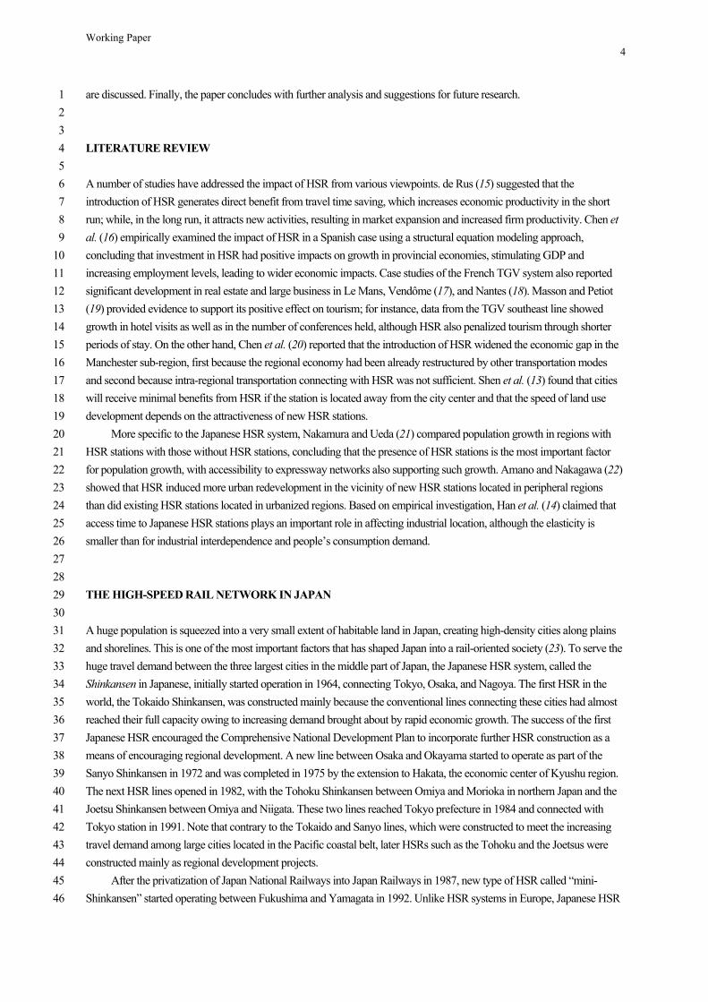
TABLE 4 shows the results of the pooling regression model, random effect model, and fixed effect model with the 28

instrumental variable (IV) method with the relevant statistical tests. Both models have sufficiently high fitness and have 29

similar estimates. This implies that the reverse causal relationship—that accessibility affects productivity—may be 30

supported, while the other way around is also possible. This is quite reasonable, because the reverse effect corresponds to 31

the fact that the inter-urban transportation infrastructure has been developed to connect regions between large cities, which 32

usually have relatively higher productivity than rural or peripheral areas. 33

Although there are no previous studies concerning the relationship between accessibility and productivity, there 34

are many studies investigating the relationship between travel time and productivity. For instance, Preston and Wall (26) 35

and Preston (27) reviewed past studies and insisted that the elasticity of productivity with respect to travel time ranges 36

between 0.12 and 0.29. Note most of the past studies estimate the elasticity with cross-sectional data. 37

The elasticity can be transformed as follows: 38

ttd

ACCdACC

ttd

ACCdACC

ACCdACC

ydy

ttd

ydyACC (2) 39

where y is the productivity, t is the travel time, ACC is the accessibility, and ACC is the elasticity of 40

productivity with respect to accessibility. ACCdACC is computed as 0.0203 with eq. (1) when tdt is 0.01, using 41

our dataset. As the elasticities of productivity with respect to accessibility estimated with the OLS model and the IV model 42

ACC are 0.226 and 0.300 respectively, as shown in TABLE 4, the elasticities of productivity with respect to travel time 43

are estimated to be 0.459 and 0.609 respectively. Our estimates may be a little higher than the maximum of the range 44

Working Paper 10

TABLE 3 Estimation Results of Pooling OLS Models, Random Effect Models, and Fixed Effect Models 1 Pooling OLS model

Model P1 Model P2 Model P3 Model P4 Estimate Std. Error t-value Estimate Std. Error t-value Estimate Std. Error t-value Estimate Std. Error t-value

Intercept 3.827 0.221 17.310 *** 3.252 0.104 31.200 *** 4.905 0.188 26.116 *** 4.897 0.189 25.939 *** ln (Acc) 0.094 0.025 3.841 *** 0.037 0.008 4.560 *** 0.084 0.008 9.955 *** 0.085 0.009 9.782 *** HSR_81 0.051 0.023 2.253 * –0.103 0.029 –3.608 *** –0.040 0.025 –1.584 –0.040 0.025 –1.598 HSR_91 0.052 0.023 2.306 * 0.057 0.025 2.254 * –0.044 0.024 –1.848 –0.043 0.024 –1.802 HSR_01 –0.055 0.022 –2.544 ** 0.144 0.024 5.980 *** 0.095 0.021 4.495 *** 0.096 0.021 4.519 *** Transfer time to largest cities –0.115 0.029 >100 *** –0.047 0.026 –1.801 –0.044 0.027 –1.629 Port and airport –0.011 0.020 –0.523 ln (Female share in their 30s) –0.782 0.078 –9.995 *** –0.783 0.078 –9.989 *** ln (GRP share of FIRE industry) 0.242 0.040 6.106 *** 0.042 0.039 1.061 0.042 0.039 1.073 Adj. R-Squared 0.413 0.514 0.636 0.634

Random effect model

Model R1 Model R2 Model R3 Model R4 Estimate Std. Error t-value Estimate Std. Error t-value Estimate Std. Error t-value Estimate Std. Error t-value

Intercept 3.710 0.088 42.200 *** 5.113 0.123 41.601 *** 4.631 0.196 23.580 *** 4.645 0.199 23.381 *** ln (Acc) 0.057 0.011 5.403 *** 0.086 0.010 8.767 *** 0.072 0.011 6.845 *** 0.072 0.011 6.701 *** HSR_81 –0.136 0.032 –4.301 *** -0.013 0.025 -0.495 -0.006 0.025 -0.245 –0.006 0.025 –0.247 HSR_91 0.069 0.030 2.277 * -0.022 0.025 -0.889 -0.002 0.026 -0.094 –0.004 0.026 –0.154 HSR_01 0.187 0.029 6.491 *** 0.127 0.023 5.425 *** 0.124 0.023 5.401 *** 0.123 0.023 5.322 *** Transfer time to largest cities -0.064 0.026 -2.428 ** -0.069 0.026 -2.633 *** –0.069 0.026 –2.618 *** Port and airport 0.006 0.023 0.264 ln (Female share in their 30s) -0.712 0.072 -9.843 0.000 –0.715 0.073 –9.842 *** ln (GRP share of FIRE industry) -0.847 0.059 -14.481 *** 0.127 0.041 3.111 0.002 0.124 0.041 3.040 *** Adj. R-Squared 0.409 0.692 0.698 0.694

Fixed effect model

Model F1 Model F2 Model F3 Model F4 Estimate Std. Error t-value Estimate Std. Error t-value Estimate Std. Error t-value Estimate Std. Error t-value

ln (Acc) 0.051 9.390 0.000 0.043 6.271 0.000 0.226 0.040 5.647 *** 0.224 0.040 5.617 *** HSR_81 0.042 0.391 0.696 0.033 1.645 0.101 0.067 0.030 2.234 * 0.074 0.031 2.424 ** HSR_91 0.041 3.571 0.000 0.033 4.849 0.000 0.083 0.032 2.604 *** 0.083 0.032 2.590 *** HSR_01 0.039 5.556 0.000 0.033 6.281 0.000 0.178 0.030 5.948 *** 0.177 0.030 5.910 *** Transfer time to largest cities –0.175 0.028 –6.148 *** –0.112 0.027 –4.099 *** –0.112 0.027 –4.096 *** Port and airport 0.033 0.028 1.165 ln (Female share in their 30s) –0.520 0.075 –6.966 *** –0.530 0.075 –7.060 *** ln (GRP share of FIRE industry) 0.349 0.038 9.112 *** 0.171 0.043 3.965 *** 0.163 0.044 3.747 ***

Adj. R-Squared 0.472 0.603 0.638 0.636

F test F = 259.3214; p < 2.2e-16 F = 299.9969; p < 2.2e-16 F = 436.3626; p < 2.2e-16 F = 307.7988; p < 2.2e-16

Breusch-Pagan test 2 = 542.5957; p < 2.2e-16 2 = 447.4598; p < 2.2e-16 2 = 585.0976; p < 2.2e-16 2 = 448.6018; p < 2.2e-16

Hausman test 2 = 294.1404; p < 2.2e-16 2 = 635.0802; p < 2.2e-16 2 = 279.9711; p < 2.2e-16 2 = 708.3238; p < 2.2e-16

Note: “***”: p<0.01; “**”: p<0.02; and “*”: p<0.05. 2

Working Paper 11

TABLE 4 Estimation Results with IV Method 1

Pooling IV model Estimate Std. Error t-value Intercept 7.003 0.200 35.043*** ln (Acc) 0.056 0.010 5.575** HSR_81 –0.023 0.026 –0.892 HSR_91 0.0004 0.026 0.014 HSR_01 0.127 0.023 5.545*** Transfer time to largest cities –0.063 0.027 –2.335* ln (Female share in their 30s) –0.636 0.086 –7.433*** ln (GRP share of FIRE industry) 0.098 0.043 2.268* Adj. R-Squared 0.624 Random effect model Estimate Std. Error t-value Intercept 6.878 0.205 33.507*** ln (Acc) 0.030 0.013 2.344** HSR_81 0.025 0.027 0.932 HSR_91 0.055 0.028 1.948 HSR_01 0.170 0.026 6.645*** Transfer time to largest cities –0.092 0.027 –3.417*** ln (Female share in their 30s) –0.585 0.078 –7.525*** ln (GRP share of FIRE industry) 0.186 0.044 4.201*** Adj. R-Squared 0.638 Fixed effect model Estimate Std. Error t-value ln (Acc) 0.300 0.151 1.989* HSR_81 0.083 0.031 2.668*** HSR_91 0.099 0.036 2.773*** HSR_01 0.192 0.038 4.990*** Transfer time to largest cities –0.117 0.028 –4.166*** ln (Female share in their 30s) –0.479 0.087 –5.483*** ln (GRP share of FIRE industry) 0.153 0.052 2.950*** Adj. R-Squared 0.638

Note 1: “***”: p<0.01; “**”: p<0.02; and “*”: p<0.05. 2 Note 2: Endogenous variable: Accessibility; Instrumental variables: Accessibility five years ago, Number of employees, ln 3

(Number of offices), GRP share of service industry, ln (Net stock of industrial water), Port dummy 4 Note 3: F test: F = 6.2224, p < 2.2e-16; Breusch-Pagan test: 2 = 82.46, p < 2.2e-16; and Hausman Test: 2 = 190.34, p < 5

2.2e-16. 6 7

8

shown by earlier studies. The parameters estimated with panel data tend to be larger those estimated with cross-sectional 9

data, because the cross-sectional data are analyzed under the assumption that there are mild or almost no fluctuations in the 10

structure of the model, while the panel data include short term fluctuations. 11

12

Scenario Analysis: Estimation of HSR’s Impact on Regional Productivity 13

According to our definition of accessibility, improvement of accessibility is not caused necessarily by the introduction of 14

HSR. Thus, to evaluate the impact only from the HSR, a simple scenario analysis is implemented where expected regional 15

productivities in the scenario where HSR exists (with-scenario) are compared with those in another scenario where no 16

HSR exists (without-scenario) using the estimated model. It is assumed that the without-scenario has the same conditions 17

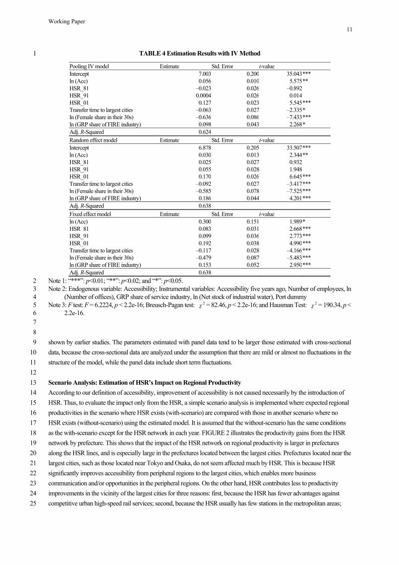
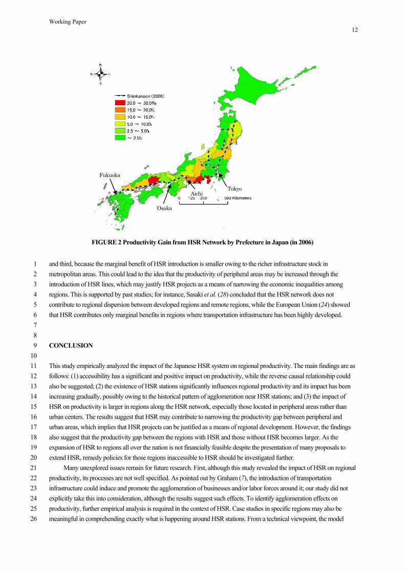
as the with-scenario except for the HSR network in each year. FIGURE 2 illustrates the productivity gains from the HSR 18

network by prefecture. This shows that the impact of the HSR network on regional productivity is larger in prefectures 19

along the HSR lines, and is especially large in the prefectures located between the largest cities. Prefectures located near the 20

largest cities, such as those located near Tokyo and Osaka, do not seem affected much by HSR. This is because HSR 21

significantly improves accessibility from peripheral regions to the largest cities, which enables more business 22

communication and/or opportunities in the peripheral regions. On the other hand, HSR contributes less to productivity 23

improvements in the vicinity of the largest cities for three reasons: first, because the HSR has fewer advantages against 24

competitive urban high-speed rail services; second, because the HSR usually has few stations in the metropolitan areas; 25

Working Paper 12

and third, because the marginal benefit of HSR introduction is smaller owing to the richer infrastructure stock in 1

metropolitan areas. This could lead to the idea that the productivity of peripheral areas may be increased through the 2

introduction of HSR lines, which may justify HSR projects as a means of narrowing the economic inequalities among 3

regions. This is supported by past studies; for instance, Sasaki et al. (28) concluded that the HSR network does not 4

contribute to regional dispersion between developed regions and remote regions, while the European Union (24) showed 5

that HSR contributes only marginal benefits in regions where transportation infrastructure has been highly developed. 6

7

8

CONCLUSION 9

10

This study empirically analyzed the impact of the Japanese HSR system on regional productivity. The main findings are as 11

follows: (1) accessibility has a significant and positive impact on productivity, while the reverse causal relationship could 12

also be suggested; (2) the existence of HSR stations significantly influences regional productivity and its impact has been 13

increasing gradually, possibly owing to the historical pattern of agglomeration near HSR stations; and (3) the impact of 14

HSR on productivity is larger in regions along the HSR network, especially those located in peripheral areas rather than 15

urban centers. The results suggest that HSR may contribute to narrowing the productivity gap between peripheral and 16

urban areas, which implies that HSR projects can be justified as a means of regional development. However, the findings 17

also suggest that the productivity gap between the regions with HSR and those without HSR becomes larger. As the 18

expansion of HSR to regions all over the nation is not financially feasible despite the presentation of many proposals to 19

extend HSR, remedy policies for those regions inaccessible to HSR should be investigated further. 20

Many unexplored issues remain for future research. First, although this study revealed the impact of HSR on regional 21

productivity, its processes are not well specified. As pointed out by Graham (7), the introduction of transportation 22

infrastructure could induce and promote the agglomeration of businesses and/or labor forces around it; our study did not 23

explicitly take this into consideration, although the results suggest such effects. To identify agglomeration effects on 24

productivity, further empirical analysis is required in the context of HSR. Case studies in specific regions may also be 25

meaningful in comprehending exactly what is happening around HSR stations. From a technical viewpoint, the model 26

Tokyo

Fukuoka

Osaka

Aichi

FIGURE 2 Productivity Gain from HSR Network by Prefecture in Japan (in 2006)

Working Paper 13

should also be elaborated further. While our study assumed that all passengers would use the minimum travel time route, 1

modal choice models can be incorporated in order to reflect the preferences of passengers in reality. 2

3

4

ACKNOWLEDGEMENT 5

6

Dataset of transportation network and level of transportation service used in our empirical study is obtained from National 7

Integrated Transport Analysis System (NITAS), which was developed by Ministry of Land, Infrastructure, Transport and 8

Tourism (MLIT), Japan. We thank them for providing the valuable data. 9

10

11

REFERENCES 12

13

1. Aschauer, D. A. Is Public Expenditure Productive? Journal of Monetary Economics, Vol. 23, 1989, pp. 177–200. 14

2. Canning, D. A Database of World Infrastructure Stocks, 1950–95. World Bank, Washington, D.C., 1998. 15

3. World Bank. World Development Report 1994. Oxford University Press, Washington, D.C., 1994. 16

4. Litman, T. Evaluating Transportation Economic Development Impacts: Understanding How Transport Policy and 17

Planning Decisions Affect Employment, Incomes, Productivity, Competitiveness, Property Values and Tax Revenues. 18

Victoria Transport Policy Institute, 2010. http://www.vtpi.org/econ_dev.pdf. Accessed on July 11, 2015. 19

5. Banister, D., and M. Thurstain-Goodwin. Quantification of the Non-transport Benefits Resulting from Rail Investment. 20

Journal of Transport Geography, Vol. 19, No. 2, 2011, pp. 212–223. 21

6. Lakshmanan, T. R. The Broader Economic Consequences of Transport Infrastructure Investments. Journal of Transport 22

Geography, Vol. 19, No. 1, 2011, pp. 1–12. 23

7. Graham, D. Agglomeration, Productivity and Transport Investment. Journal of Transport Economics and Policy, Vol. 41, 24

No.3, 2007, pp. 317–343. 25

8. Chatman, D. G., and R. B. Noland. Do Public Transport Improvements Increase Agglomeration Economies? A Review 26

of Literature and an Agenda for Research. Transport Reviews, Vol. 31, No. 6, 2011, pp. 725–742. 27

9. Deng, T. Impacts of Transport Infrastructure on Productivity and Economic Growth: Recent Advances and Research 28

Challenges. Transport Reviews, Vol. 33, No. 6, 2013, pp. 686–699. 29

10. Keeble, D., P. Owens, and C. Thompson. Regional Accessibility and Economic Potential in the European Community. 30

Regional Studies, Vol. 16, 1982, pp. 419–432. 31

11. Cao, J., X. C. Liu, Y. Wang, and Q. Li. Accessibility Impacts of China’s High-speed Rail Network. Journal of Transport 32

Geography, Vol. 28, 2013, pp. 12–21. 33

12. Dobruszkes, F. High-speed Rail and Air Transport Competition in Western Europe: A Supply-oriented Perspective. 34

Transport Policy, Vol. 18, 2011, pp. 870–879. 35

13. Shen, Y., J. D. A. E. Silva, and L. M. Martínez. HSR Station Location Choice and its Local Land Use Impacts on Small 36

Cities: A Case Study of Aveiro, Portugal. Procedia - Social and Behavioral Sciences, Vol. 111, 2014, pp. 470–479. 37

14. Han, J., Y. Hayashi, P. Jia, and Q. Yuan. Economic Effect of High-Speed Rail: Empirical Analysis of Shinkansen’s 38

Impact on Industrial Location. Journal of Transportation Engineering, Vol. 138, No. 12, 2012, pp. 1551–1557. 39

15. de Rus, G. ed. Economic Analysis of High Speed Rail in Europe, Revised Version, Bilbao: Fundación BBVA, 2012. 40

16. Chen, G., and J. D. A. E. Silva. Estimating the Provincial Economic Impacts of High-speed Rail in Spain: An Application 41

of Structural Equation Modeling. Procedia - Social and Behavioral Sciences, Vol. 111, 2014, pp. 157–165. 42

17. Pieda. Rail Link Project: A Comparative Appraisal of Socio-Economic and Development Impacts of Alternative Routes. 43

Pieda, Reading, 1991. 44

18. Sands, B. D. The Development Effects of High-Speed Rail Stations and Implications for California. Built Environment, 45

Vol. 19 1993, pp. 257–284. 46

Working Paper 14

19. Masson, S., and R. Petiot. Can The High Speed Rail Reinforce Tourism Attractiveness? The Case of the High Speed 1

Rail Between Perpignan (France) and Barcelona (Spain). Technovation, Vol. 29, 2009, pp. 611–617. 2

20. Chen, C.-L., and P. Hall. The Wider Spatial-economic Impacts of High-speed Trains: A Comparative Case Study of 3

Manchester and Lille Sub-regions. Journal of Transport Geography, Vol. 24, 2012, pp. 89–110. 4

21. Nakamura, H., and T. Ueda. The Impacts of the Shinkansen on Regional Development. Presented at the Fifth World 5

Conference on Transport Research, Yokohama, Vol. III, Western Periodicals, Ventura, California, 1989. 6

22. Amano, K., and D. Nakagawa. Study on Urbanization Impacts by New Stations of High Speed Railway. Presented at 7

the Conference of the Korean Transportation Association, Dejeon City, 1990. 8

23. Okada, H. Features and Economic and Social Effect of the Shinkansen. Japan Railway & Transport Review, October 9

1994, pp. 9–16. 10

24. European Union. Transport Accessibility at Regional/Local Scale and Patterns in Europe. 2013. 11

http://www.espon.eu/export/sites/default/Documents/Projects/AppliedResearch/TRACC/FR/TRACC_FR_Volume212

_ScientificReport.pdf. Accessed on July 11, 2015. 13

25. Rao, S., S. Andrew, and T. Jianmin. Productivity Growth in Service Industries: A Canadian Success Story. 2004. 14

http://www.csls.ca/reports/ProdServiceIndustries.pdf. Accessed on July 11, 2015. 15

26. Preston, J., and G. Wall. The Ex-ante and Ex-post Economic and Social Impacts of the Introduction of High-speed Trains 16

in South East England. Planning Practice and Research, Vol. 23, No. 3, 2008, pp. 403–422. 17

27. Preston, J. The Case for High Speed Rail: A Review of Recent Evidence. Royal Automobile Club Foundation for 18

Motoring No. 09/128, 2009, pp. 1–29. 19

28. Sasaki, K., T. Ohashi, and A. Ando. High-speed Rail Transit Impact on Regional Systems: Does the Shinkansen 20

Contribute to Dispersion? The Annals of Regional Science, Vol. 31, No. 1, 1997, pp. 77–98. 21