word embeddings - w4nderlustw4nderlu.st/content/4-teaching/3-word-embeddings/... · word...

Past, Present and Future

Piero Molino

Word Embeddings

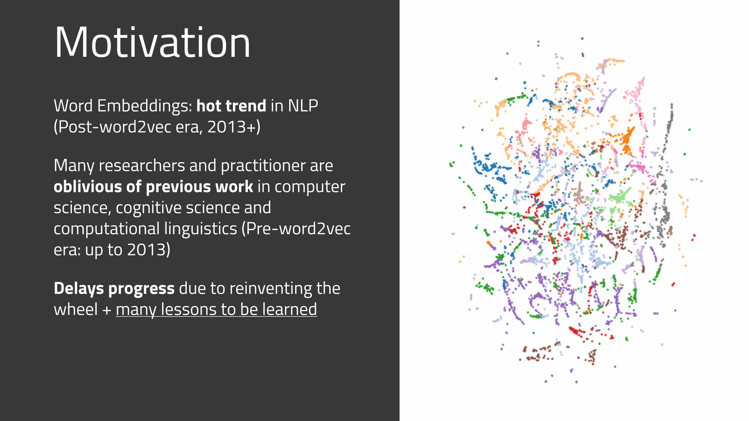
MotivationWord Embeddings: hot trend in NLP (Post-word2vec era, 2013+)

Many researchers and practitioner are oblivious of previous work in computer science, cognitive science and computational linguistics (Pre-word2vec era: up to 2013)

Delays progress due to reinventing the wheel + many lessons to be learned

Goal

Overview* of the history of the field to start building on existing knowledge

Give some hints on future directions

*Not complete overview, but a useful starting point for exploration

Outline

1. Linguistic background: Structuralism

2. Distributional Semantics

3. Methods overview

4. Open issues and current trends

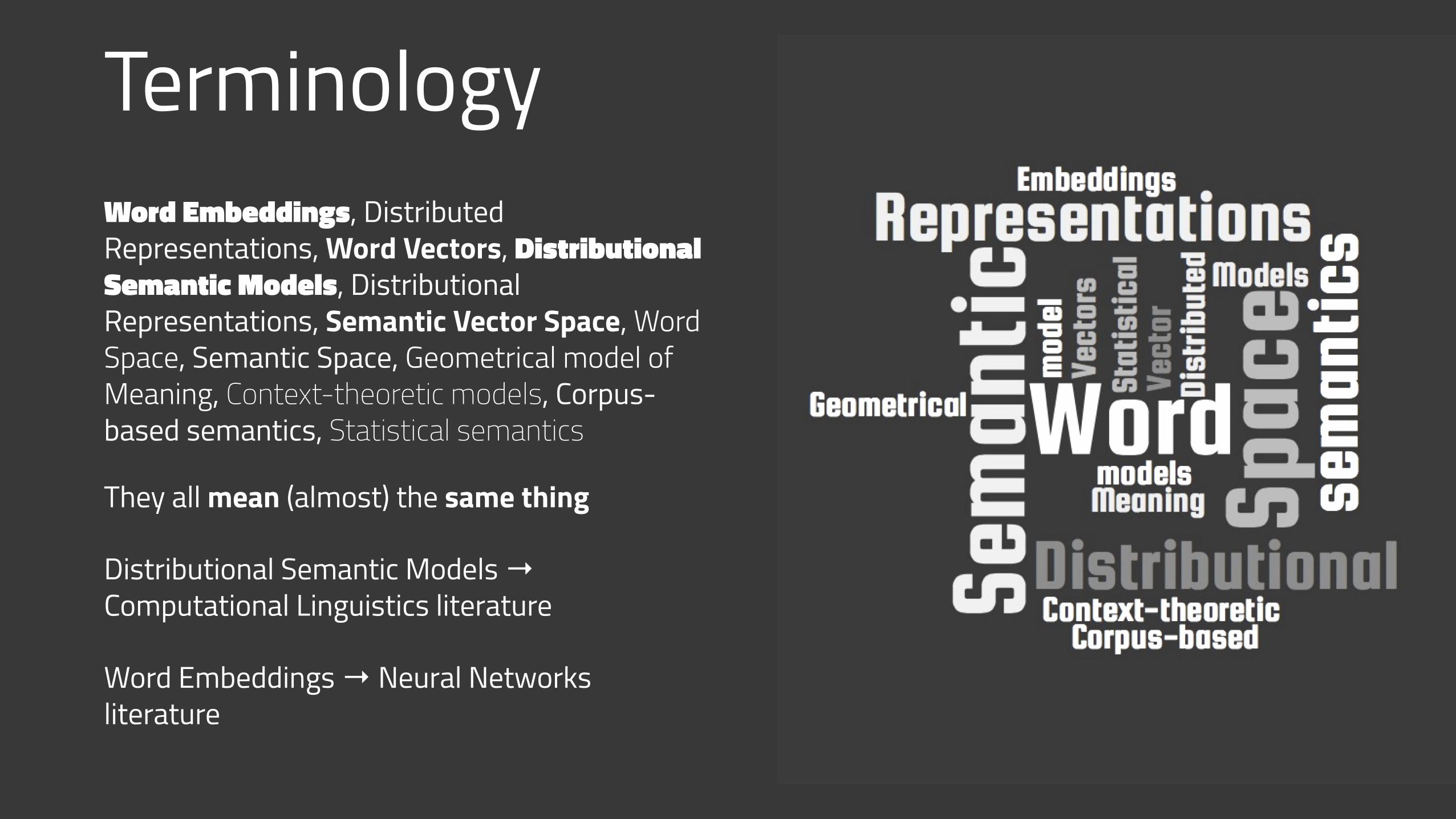
TerminologyWord Embeddings, Distributed Representations, Word Vectors, Distributional Semantic Models, Distributional Representations, Semantic Vector Space, Word Space, Semantic Space, Geometrical model of Meaning, Context-theoretic models, Corpus-based semantics, Statistical semantics

They all mean (almost) the same thing

Distributional Semantic Models → Computational Linguistics literature

Word Embeddings → Neural Networks literature

Structuralism

- Simon Blackburn, Oxford Dictionary of Philosophy, 2008

“The belief that phenomena of human life are not intelligible except through their interrelations.

These relations constitute a structure, and behind local variations in the surface phenomena

there are constant laws of abstract culture”

Structuralism

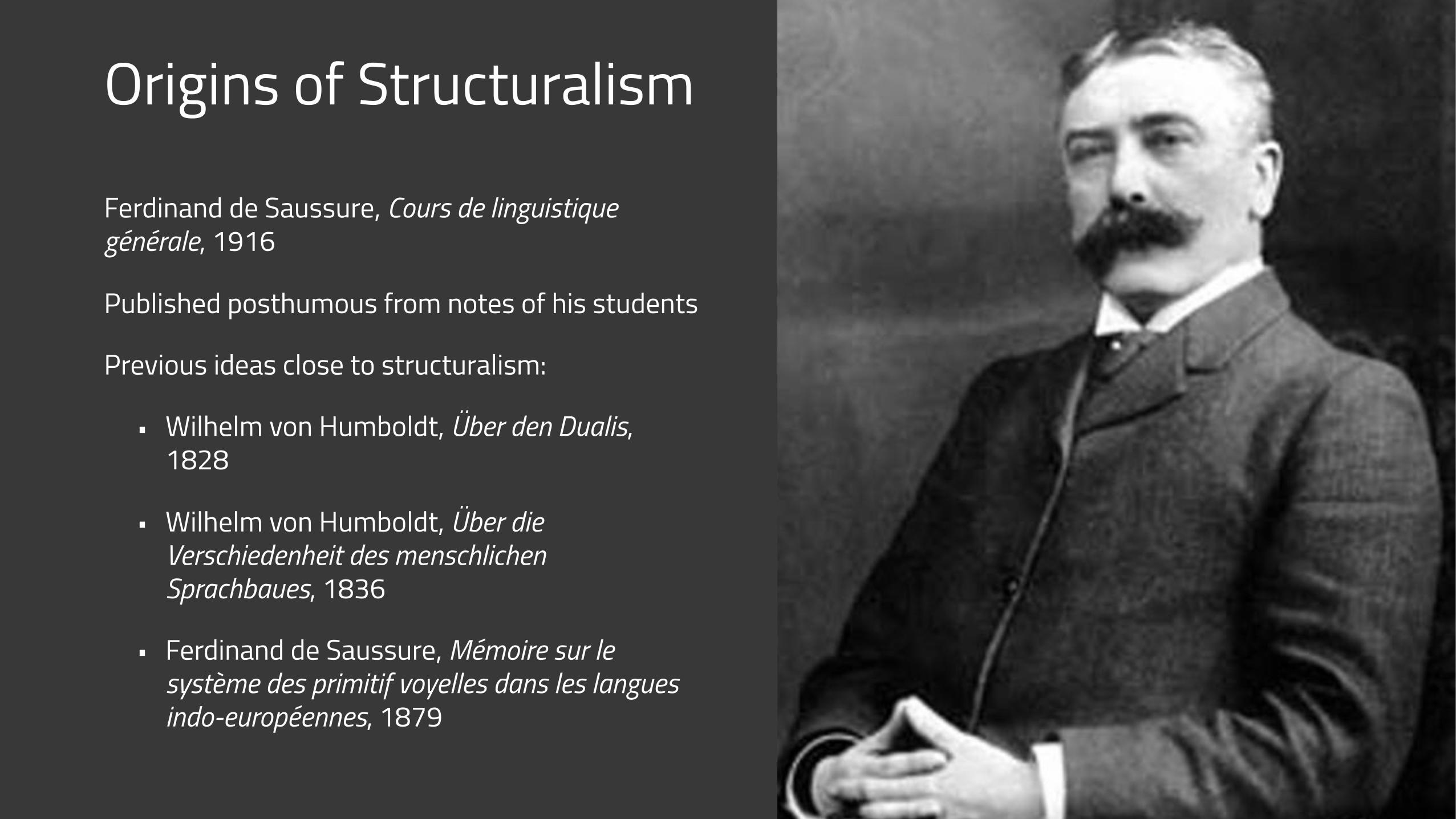
Origins of Structuralism

Ferdinand de Saussure, Cours de linguistique générale, 1916

Published posthumous from notes of his students

Previous ideas close to structuralism:

• Wilhelm von Humboldt, Über den Dualis, 1828

• Wilhelm von Humboldt, Über die Verschiedenheit des menschlichen Sprachbaues, 1836

• Ferdinand de Saussure, Mémoire sur le système des primitif voyelles dans les langues indo-européennes, 1879

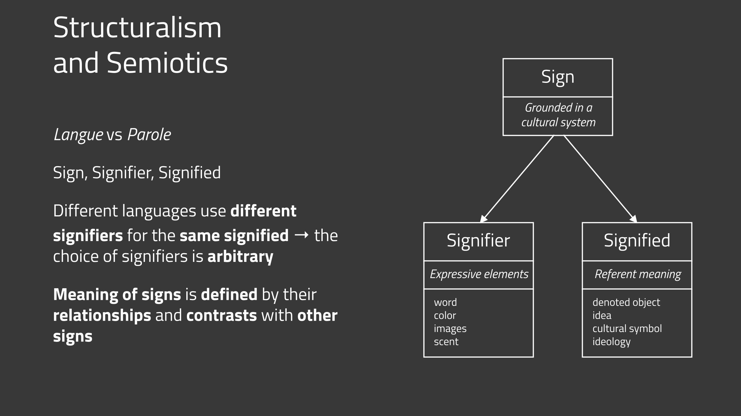
Structuralism and Semiotics

Langue vs Parole

Sign, Signifier, Signified

Different languages use different signifiers for the same signified → the choice of signifiers is arbitrary

Meaning of signs is defined by their relationships and contrasts with other signs

SignGrounded in a

cultural system

SignifierExpressive elements

word color images scent

SignifiedReferent meaning

denoted object idea cultural symbol ideology

Meaning of signs is defined by their relationships and contrasts with other signs

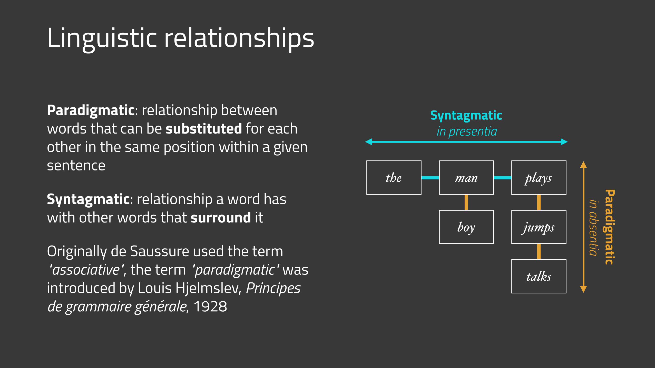
Linguistic relationships

Paradigmatic: relationship between words that can be substituted for each other in the same position within a given sentence

Syntagmatic: relationship a word has with other words that surround it

Originally de Saussure used the term "associative", the term "paradigmatic" was introduced by Louis Hjelmslev, Principes de grammaire générale, 1928

the plays

boy jumps

talks

man

Syntagmatic in presentia

Paradigmatic

in absentia

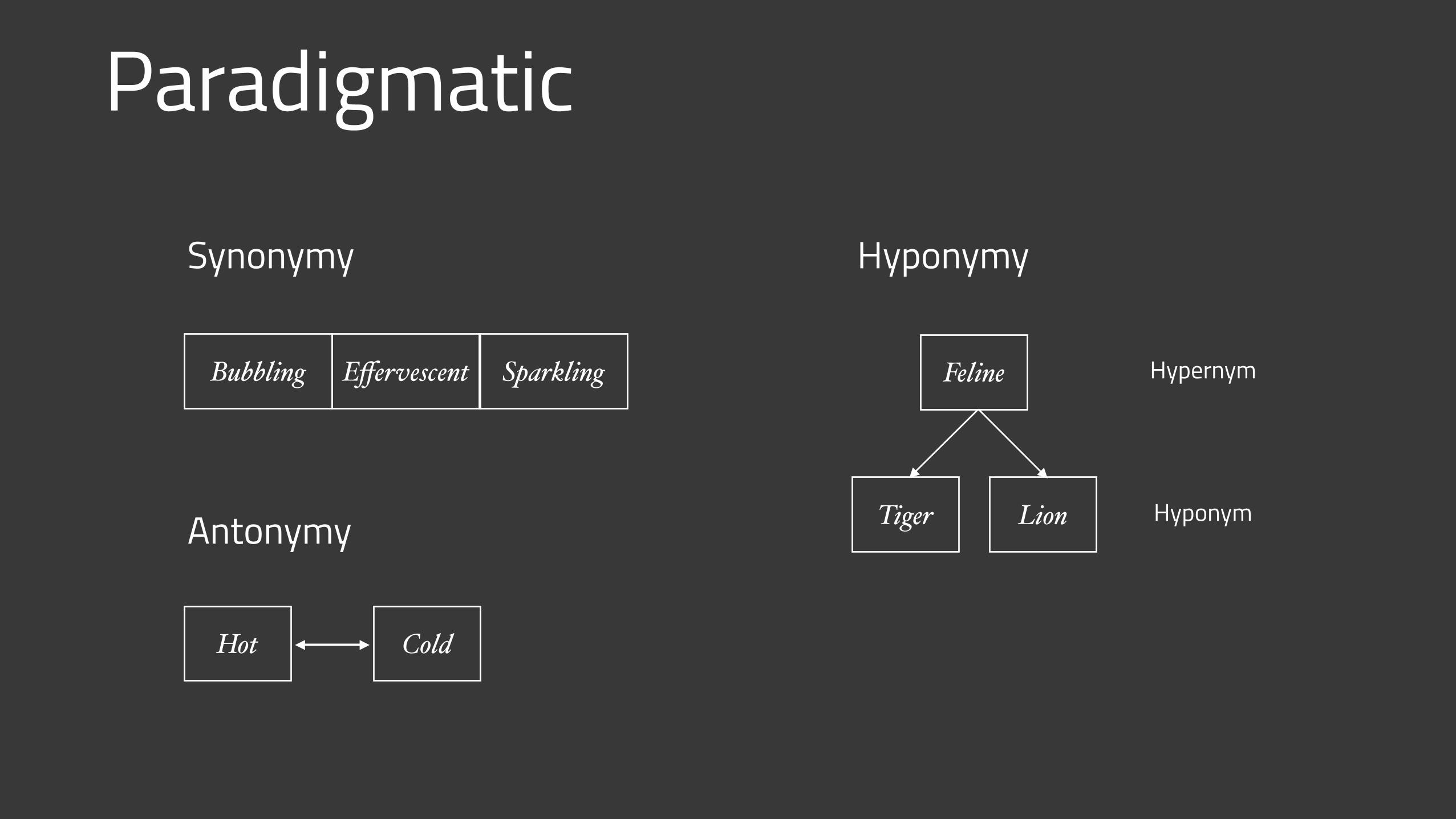
Paradigmatic

HyponymySynonymy

Antonymy

Feline

Tiger Lion Hyponym

HypernymBubbling Effervescent Sparkling

Hot Cold

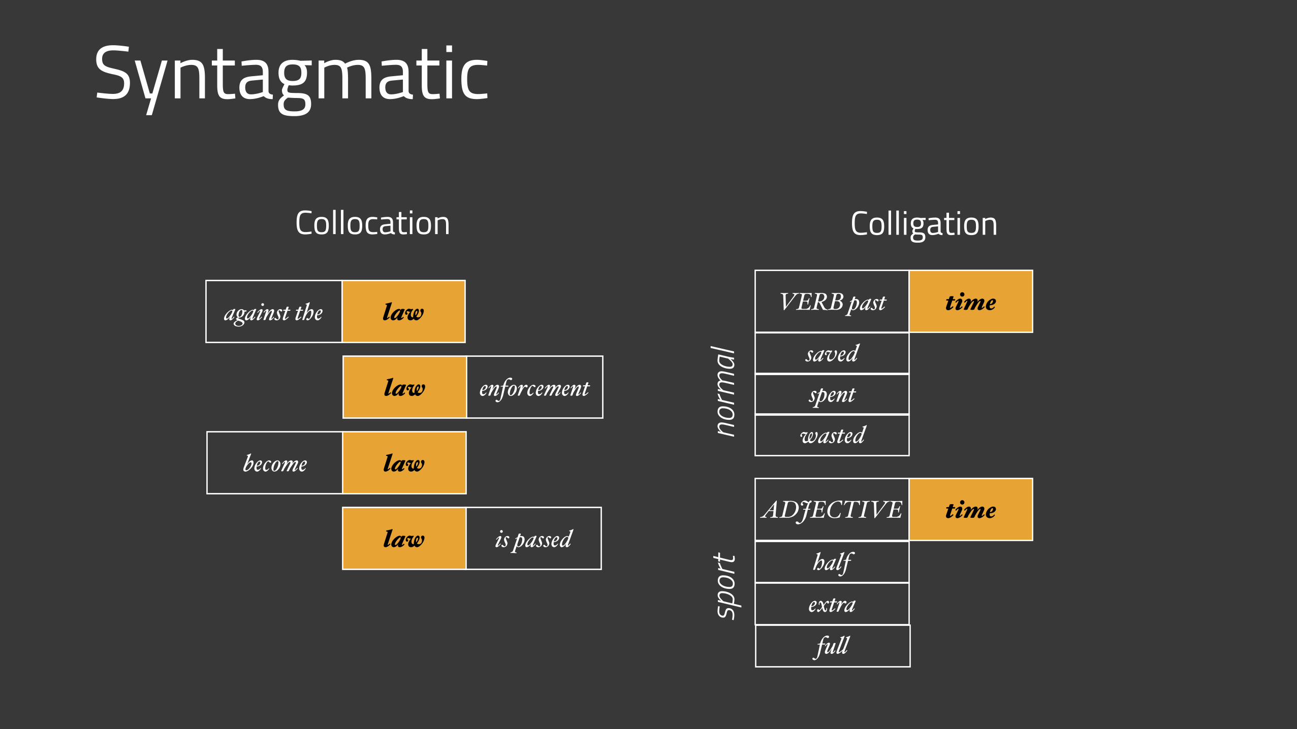
Syntagmatic

Collocation Colligation

against the law

become law

enforcementlaw

is passedlaw

VERB past time

saved

ADJECTIVE time

spentwasted

halfextrafull

spor

tno

rmal

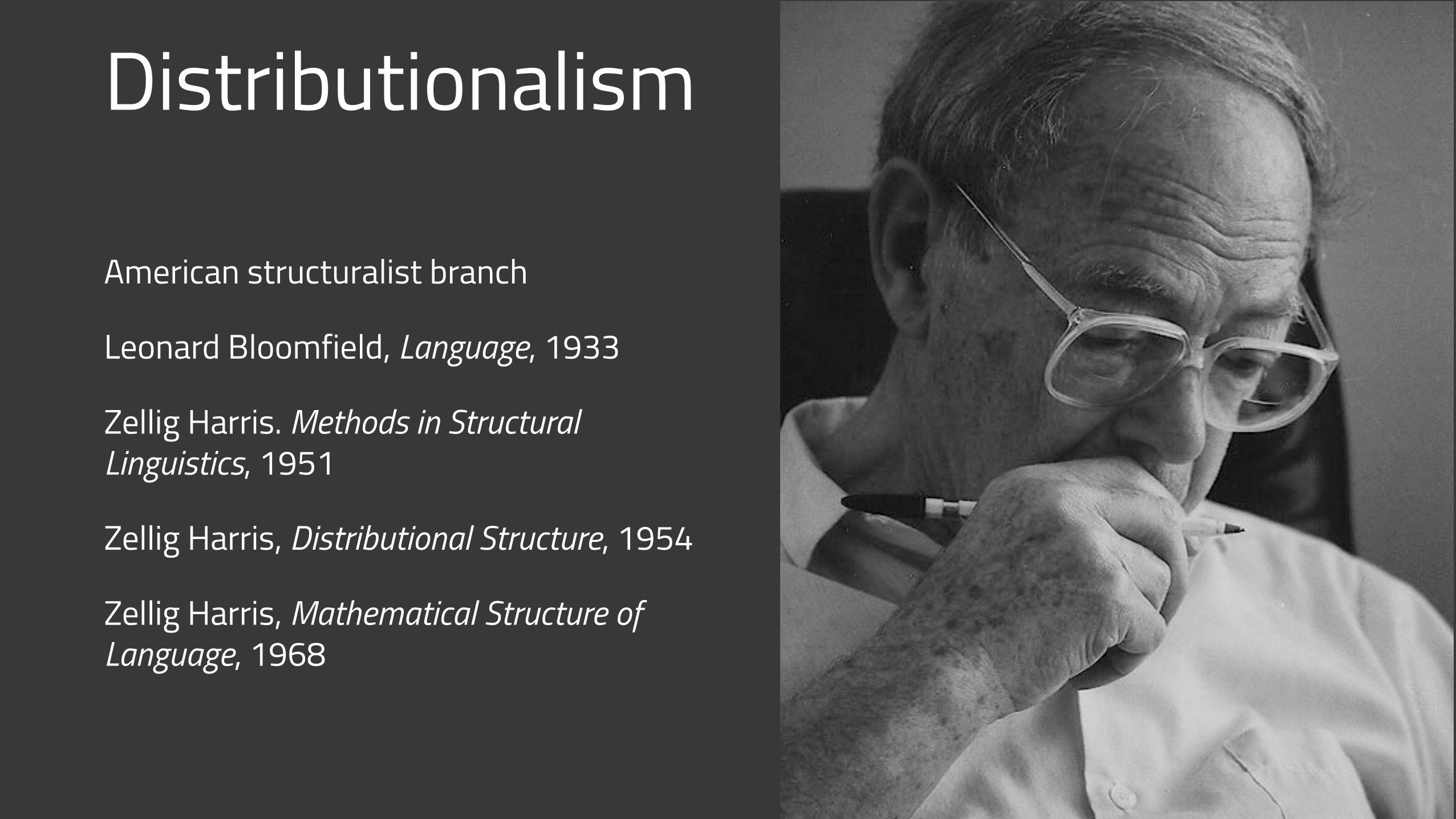
Distributionalism

American structuralist branch

Leonard Bloomfield, Language, 1933

Zellig Harris. Methods in Structural Linguistics, 1951

Zellig Harris, Distributional Structure, 1954

Zellig Harris, Mathematical Structure of Language, 1968

- Ludwig Wittgenstein, Philosophical Investigation, 1953

"The meaning of a word is its use in the language"

Philosophy of Language

- J.R. Firth, Papers in Linguistics,1957

"You shall know a word by the company it keeps"

Corpus Linguistics

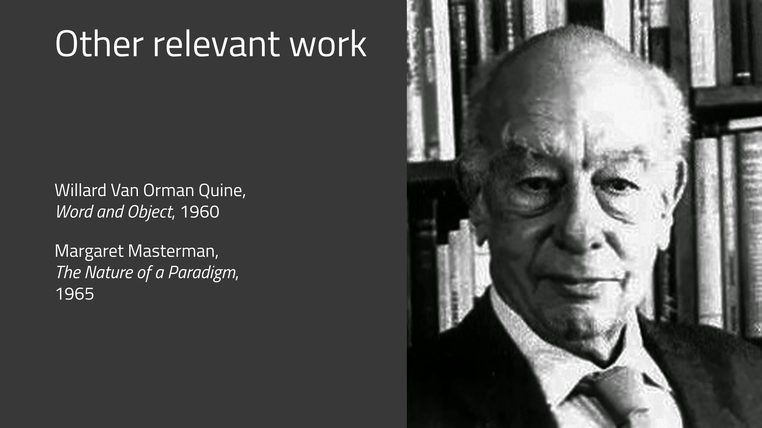
Other relevant work

Willard Van Orman Quine, Word and Object, 1960

Margaret Masterman, The Nature of a Paradigm, 1965

Distributional Semantics

Distributional Hypothesis

The degree of semantic similarity between two linguistic expressions A and B is a function of the similarity of the linguistic contexts in which A and B can appear

First formulation by Harris, Charles, Miller, Firth or Wittgenstein?

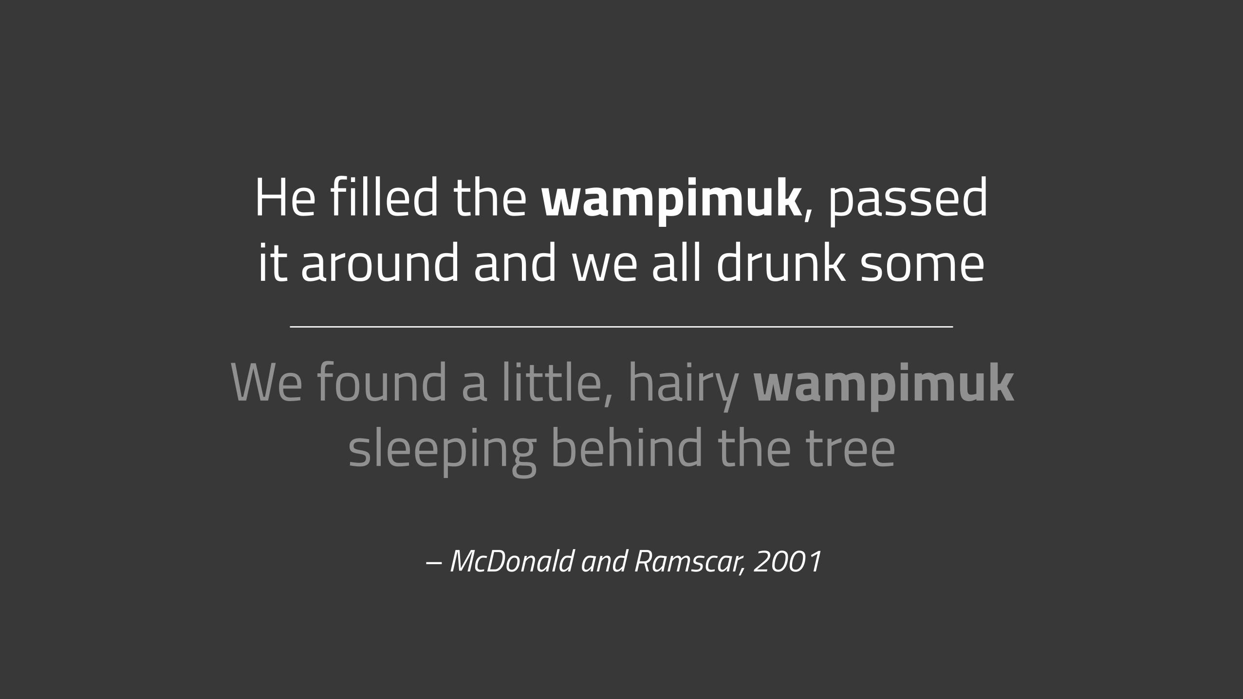
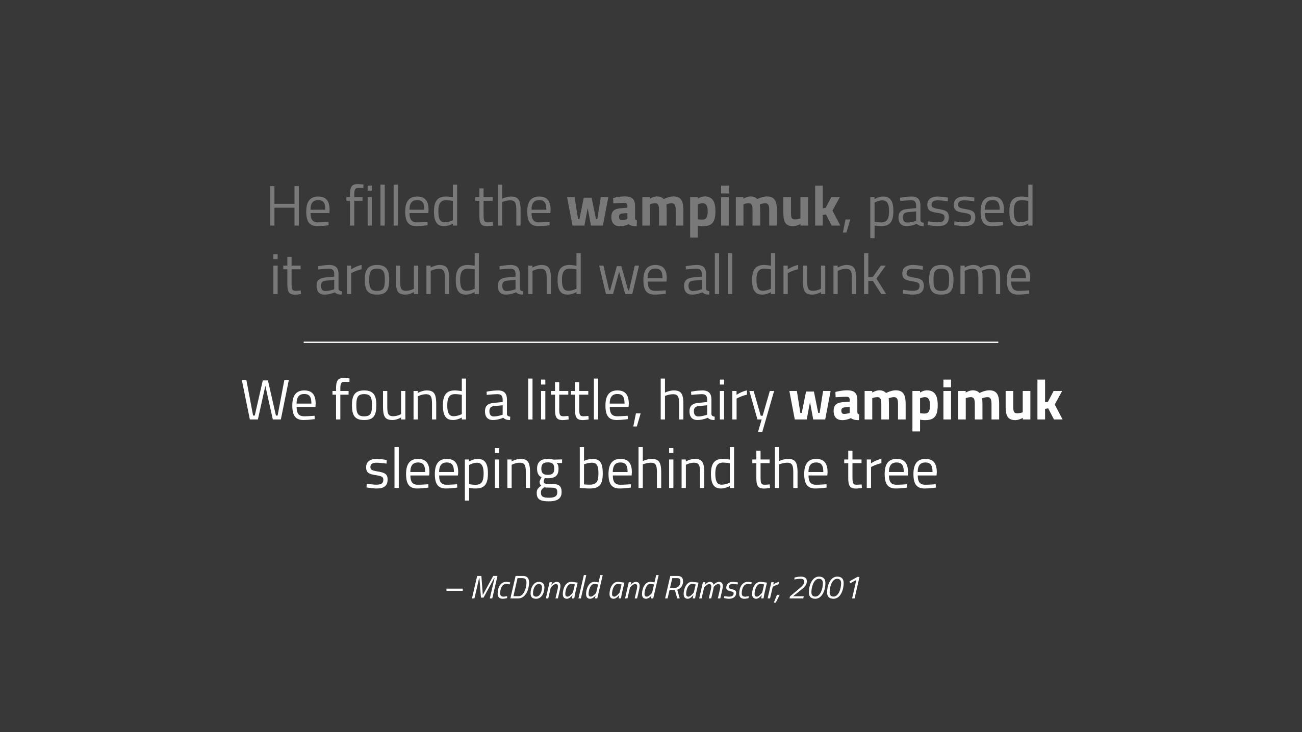
– McDonald and Ramscar, 2001

We found a little, hairy wampimuk sleeping behind the tree

He filled the wampimuk, passed it around and we all drunk some

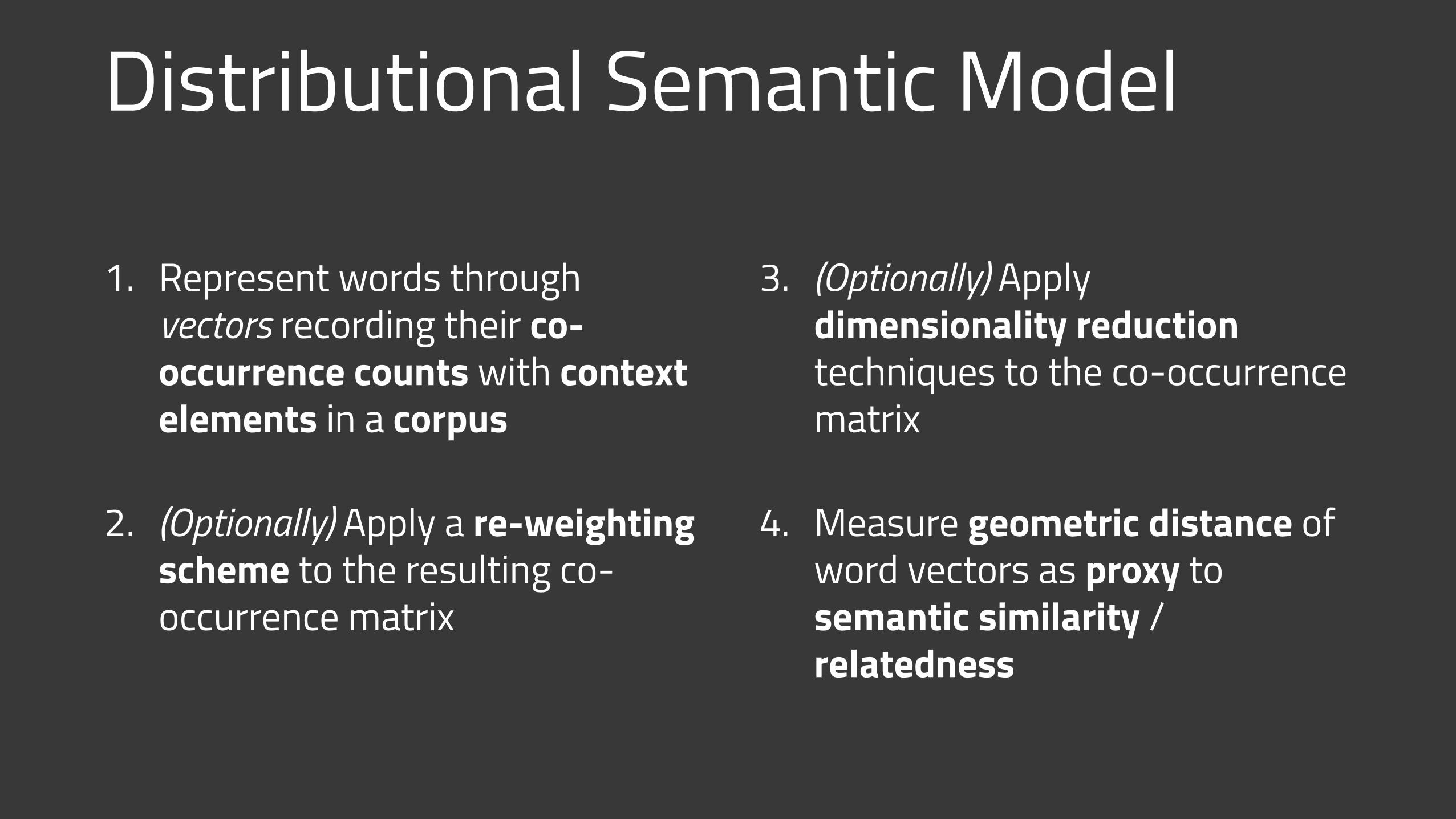
Distributional Semantic Model

1. Represent words through vectors recording their co-occurrence counts with context elements in a corpus

2. (Optionally) Apply a re-weighting scheme to the resulting co-occurrence matrix

3. (Optionally) Apply dimensionality reduction techniques to the co-occurrence matrix

4. Measure geometric distance of word vectors as proxy to semantic similarity / relatedness

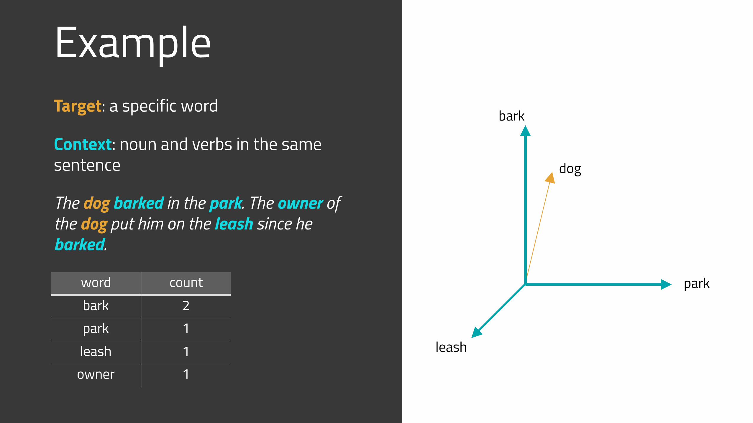
ExampleTarget: a specific word

Context: noun and verbs in the same sentence

The dog barked in the park. The owner of the dog put him on the leash since he barked.

word countbark 2park 1leash 1

owner 1

bark

leash

park

dog

ContextsTa

rget

s

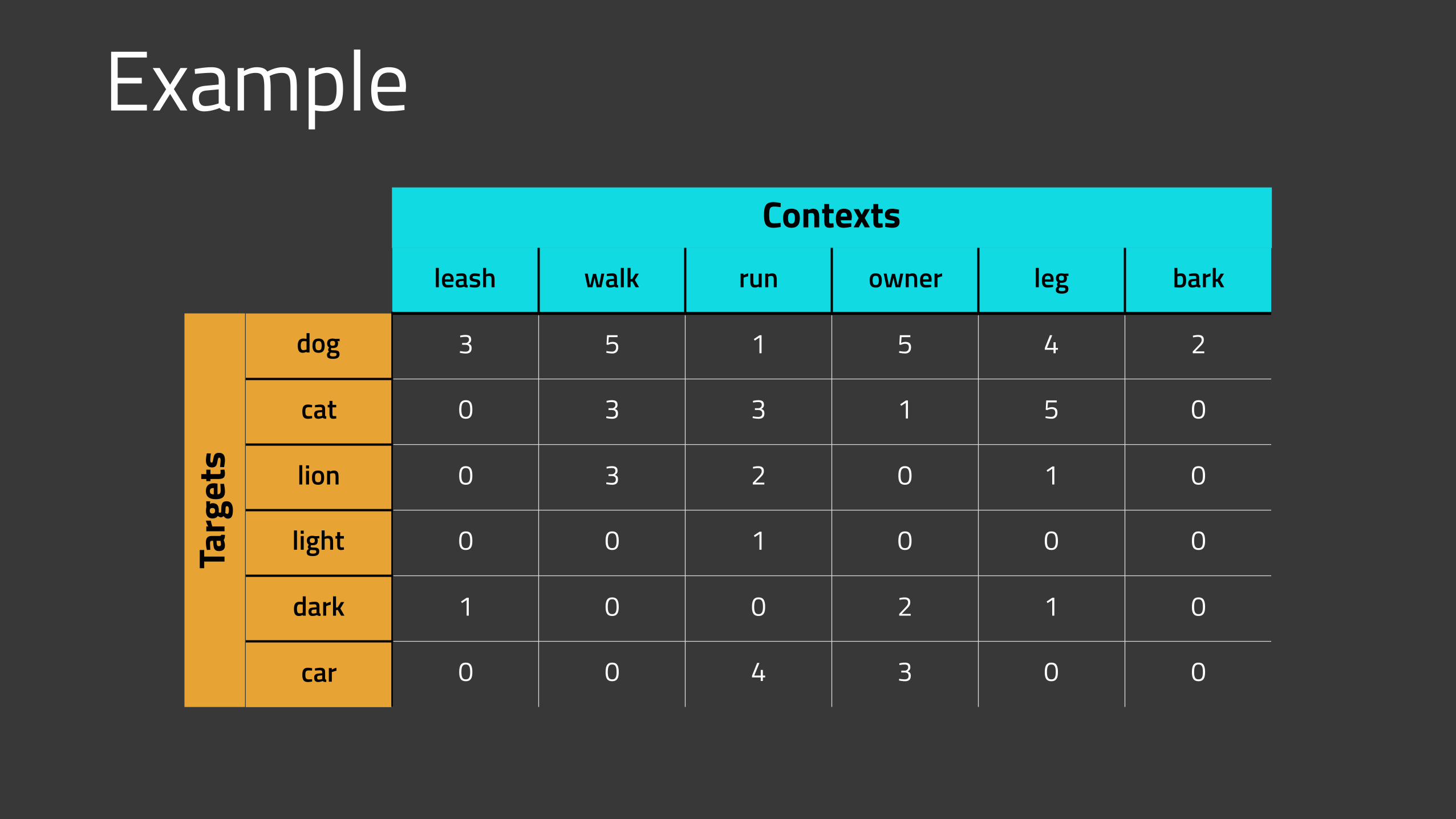
Example

leash walk run owner leg bark

dog 3 5 1 5 4 2

cat 0 3 3 1 5 0

lion 0 3 2 0 1 0

light 0 0 1 0 0 0

dark 1 0 0 2 1 0

car 0 0 4 3 0 0

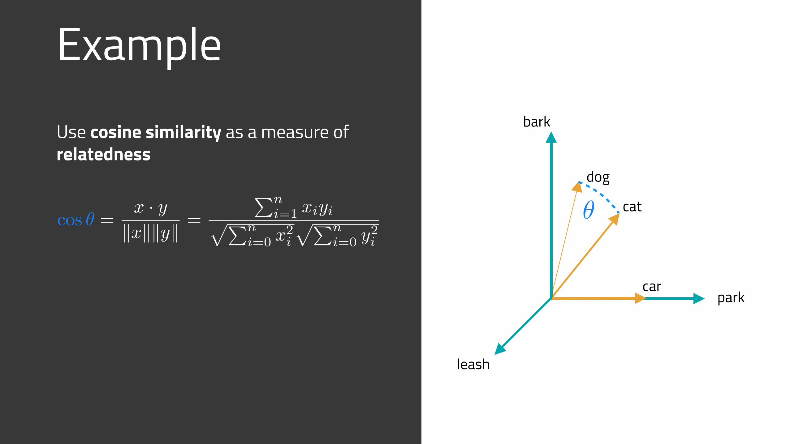
ExampleUse cosine similarity as a measure of relatedness

bark

leash

park

dog

cat

car

cos ✓ =x · y

kxkkyk =

Pni=1 xiyipPn

i=0 x2i

pPni=0 y

2i

✓cos ✓

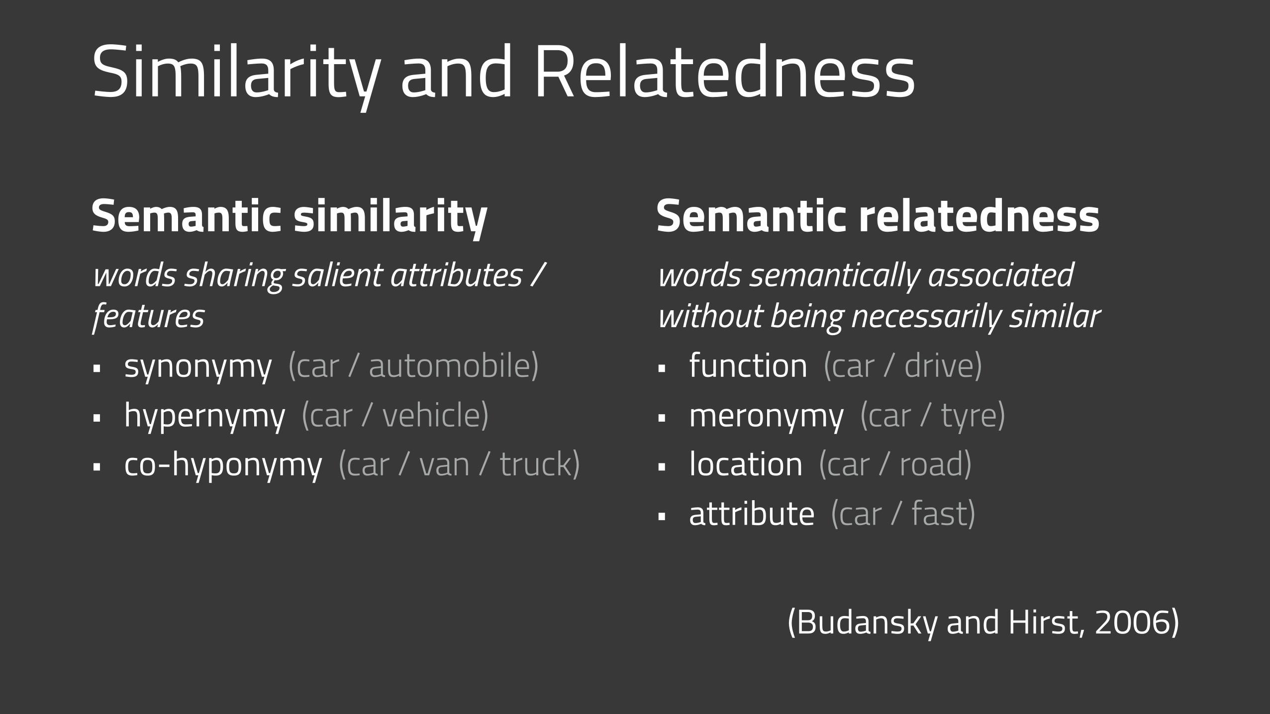
Similarity and Relatedness

Semantic similarity words sharing salient attributes / features • synonymy (car / automobile) • hypernymy (car / vehicle) • co-hyponymy (car / van / truck)

Semantic relatedness words semantically associated without being necessarily similar • function (car / drive) • meronymy (car / tyre) • location (car / road) • attribute (car / fast)

(Budansky and Hirst, 2006)

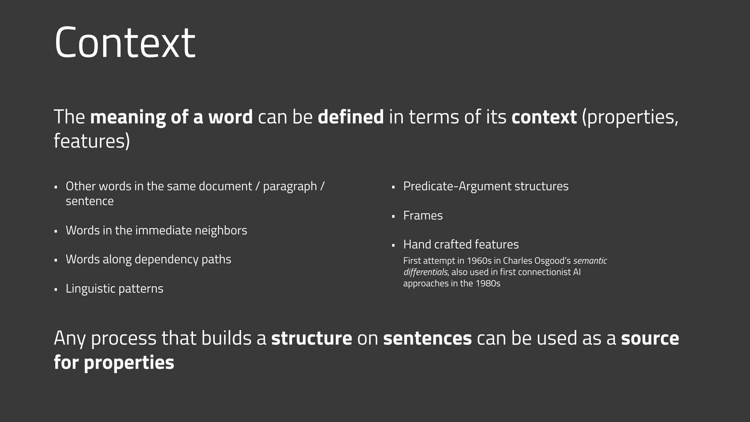
ContextThe meaning of a word can be defined in terms of its context (properties, features)

• Other words in the same document / paragraph /sentence

• Words in the immediate neighbors

• Words along dependency paths

• Linguistic patterns

• Predicate-Argument structures

• Frames

• Hand crafted features

Any process that builds a structure on sentences can be used as a source for properties

First attempt in 1960s in Charles Osgood’s semantic differentials, also used in first connectionist AI approaches in the 1980s

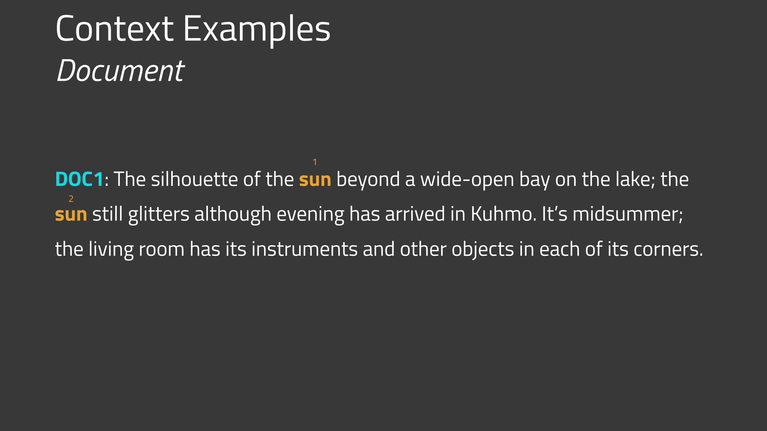
Context Examples Document

DOC1: The silhouette of the sun beyond a wide-open bay on the lake; the sun still glitters although evening has arrived in Kuhmo. It’s midsummer; the living room has its instruments and other objects in each of its corners.

1

2

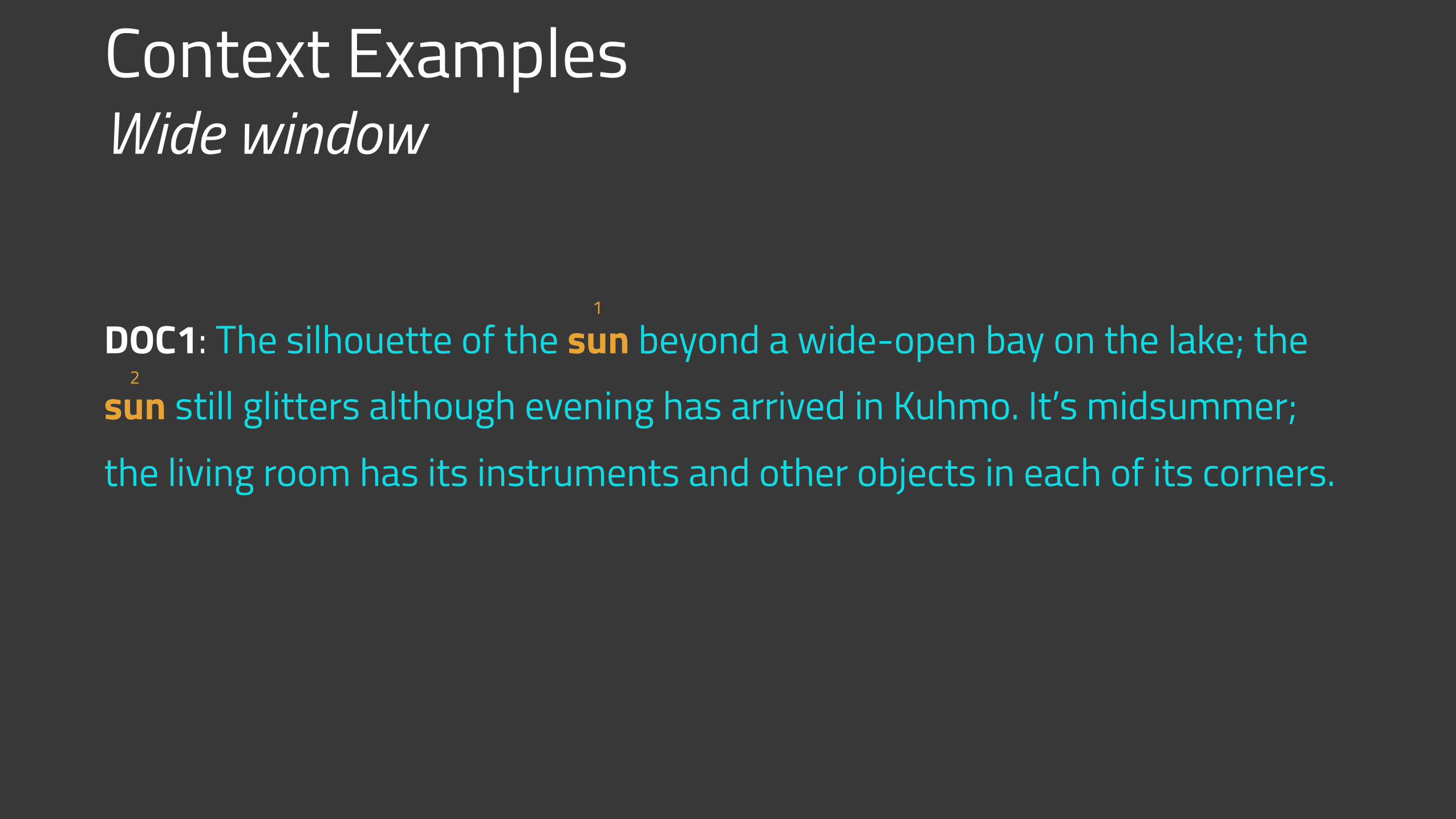
Context Examples Wide window


1

2

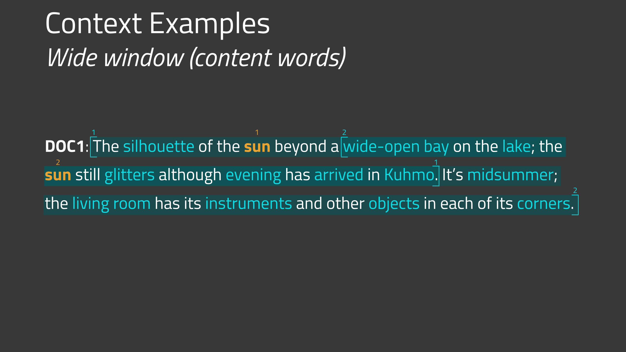
Context Examples Wide window (content words)


1

1

2

2

1

2

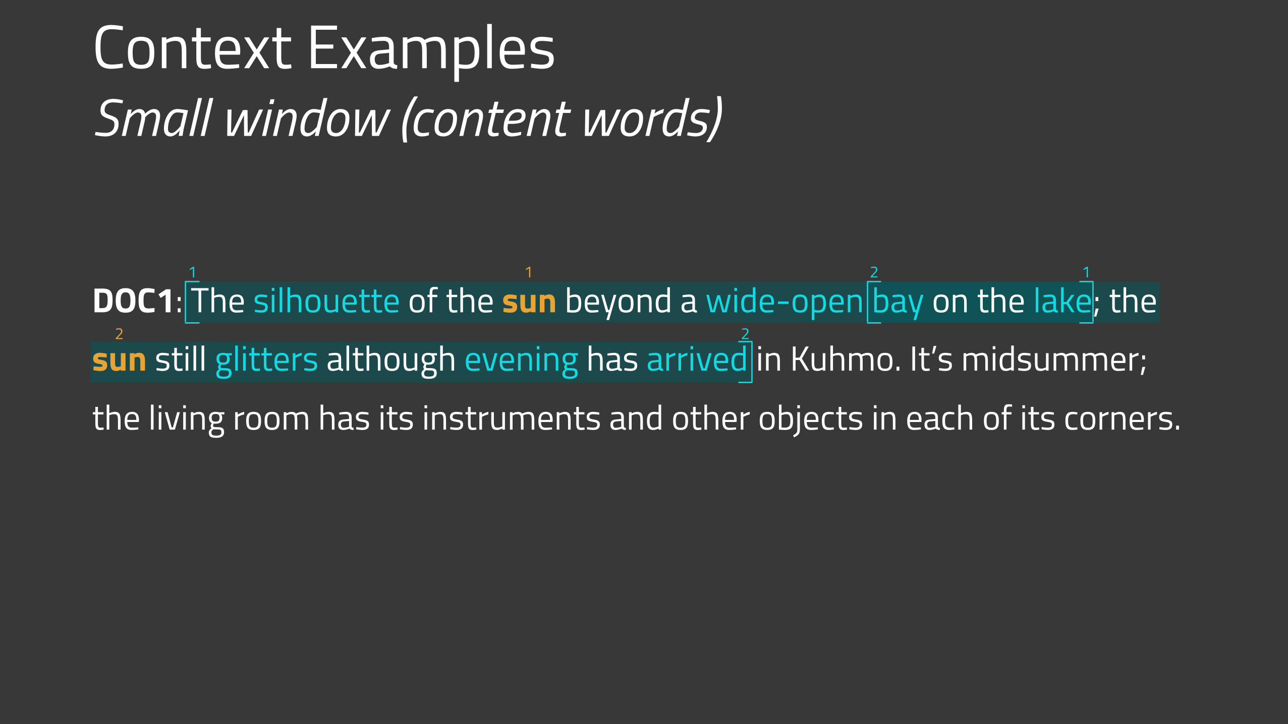
Context Examples Small window (content words)


1 12

2

1

2

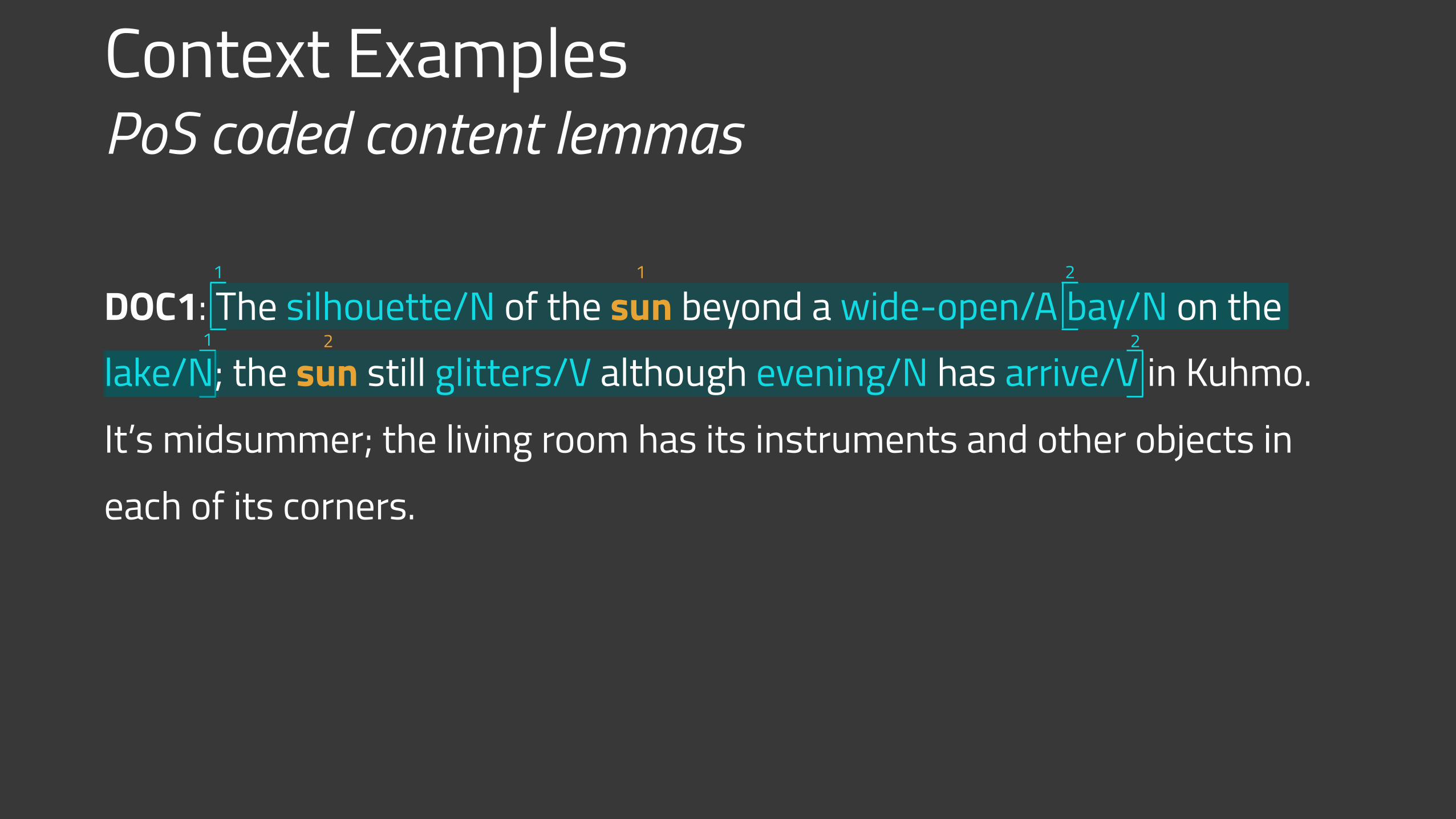
Context Examples PoS coded content lemmas

1

1

2

2

1

2DOC1: The silhouette/N of the sun beyond a wide-open/A bay/N on the lake/N; the sun still glitters/V although evening/N has arrive/V in Kuhmo. It’s midsummer; the living room has its instruments and other objects in each of its corners.

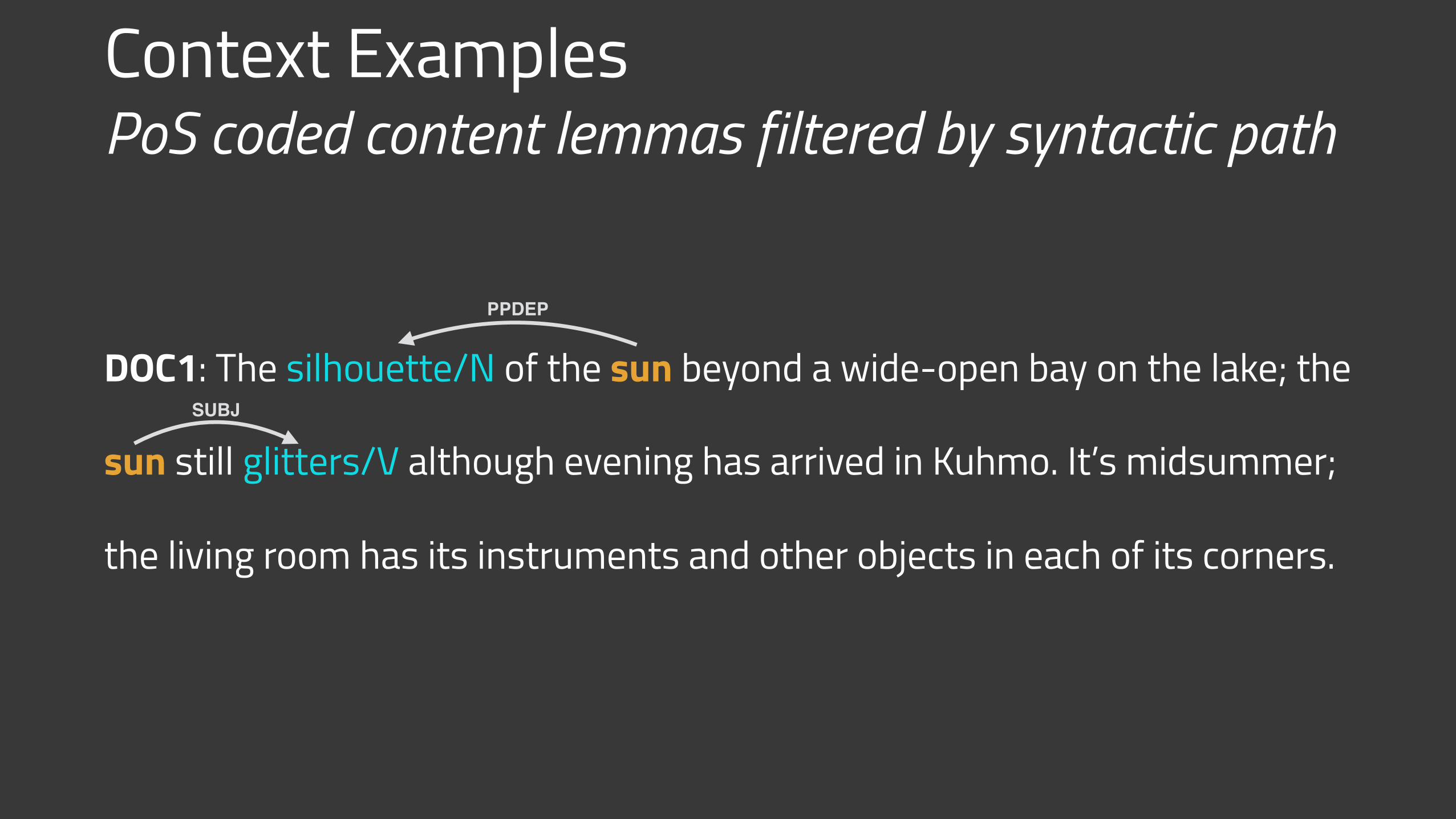
Context Examples PoS coded content lemmas filtered by syntactic path

DOC1: The silhouette/N of the sun beyond a wide-open bay on the lake; the

sun still glitters/V although evening has arrived in Kuhmo. It’s midsummer;

the living room has its instruments and other objects in each of its corners.

PPDEP

SUBJ

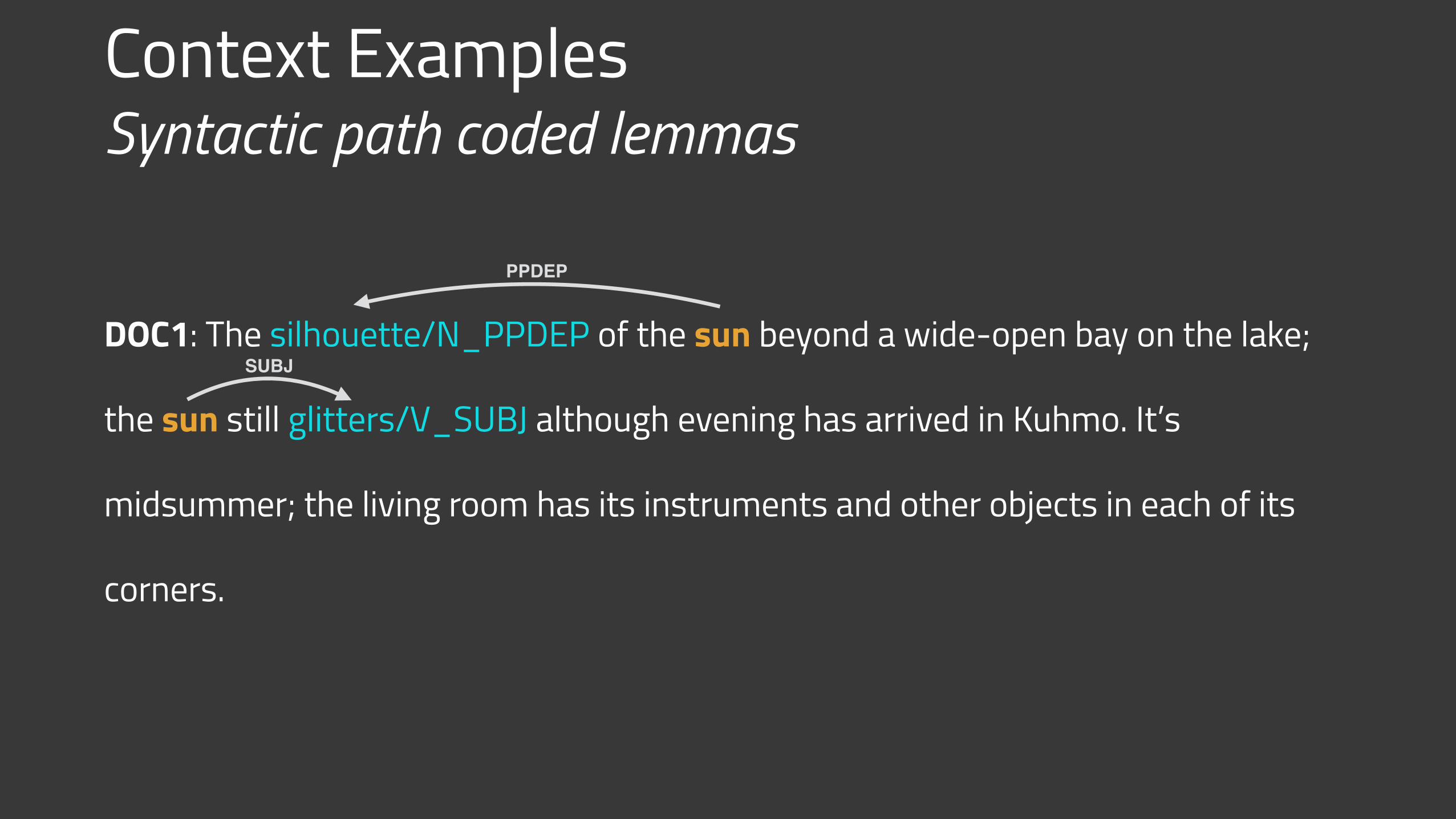
Context Examples Syntactic path coded lemmas

DOC1: The silhouette/N_PPDEP of the sun beyond a wide-open bay on the lake;

the sun still glitters/V_SUBJ although evening has arrived in Kuhmo. It’s

midsummer; the living room has its instruments and other objects in each of its

corners.

PPDEP

SUBJ

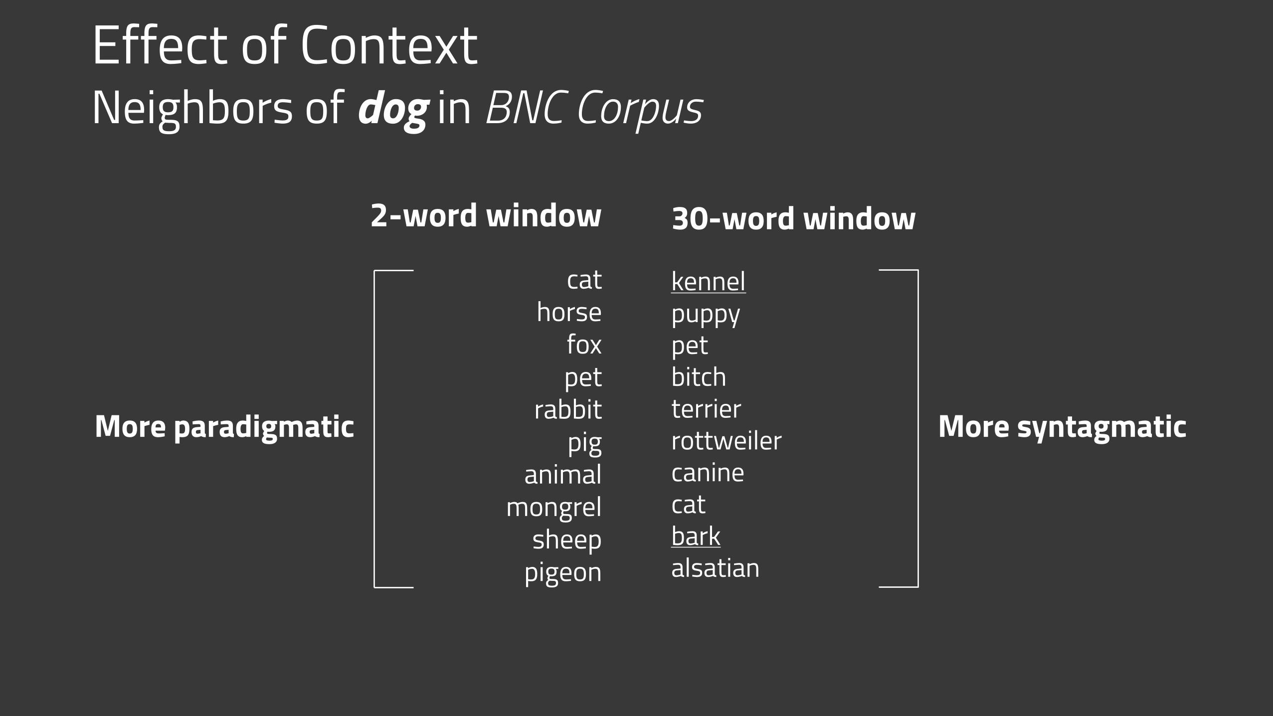
Effect of Context Neighbors of dog in BNC Corpus

2-word window

cathorse

foxpet

rabbitpig

animal mongrel

sheeppigeon

More paradigmatic More syntagmatic

30-word window

kennel puppy petbitch terrierrottweiler caninecatbarkalsatian

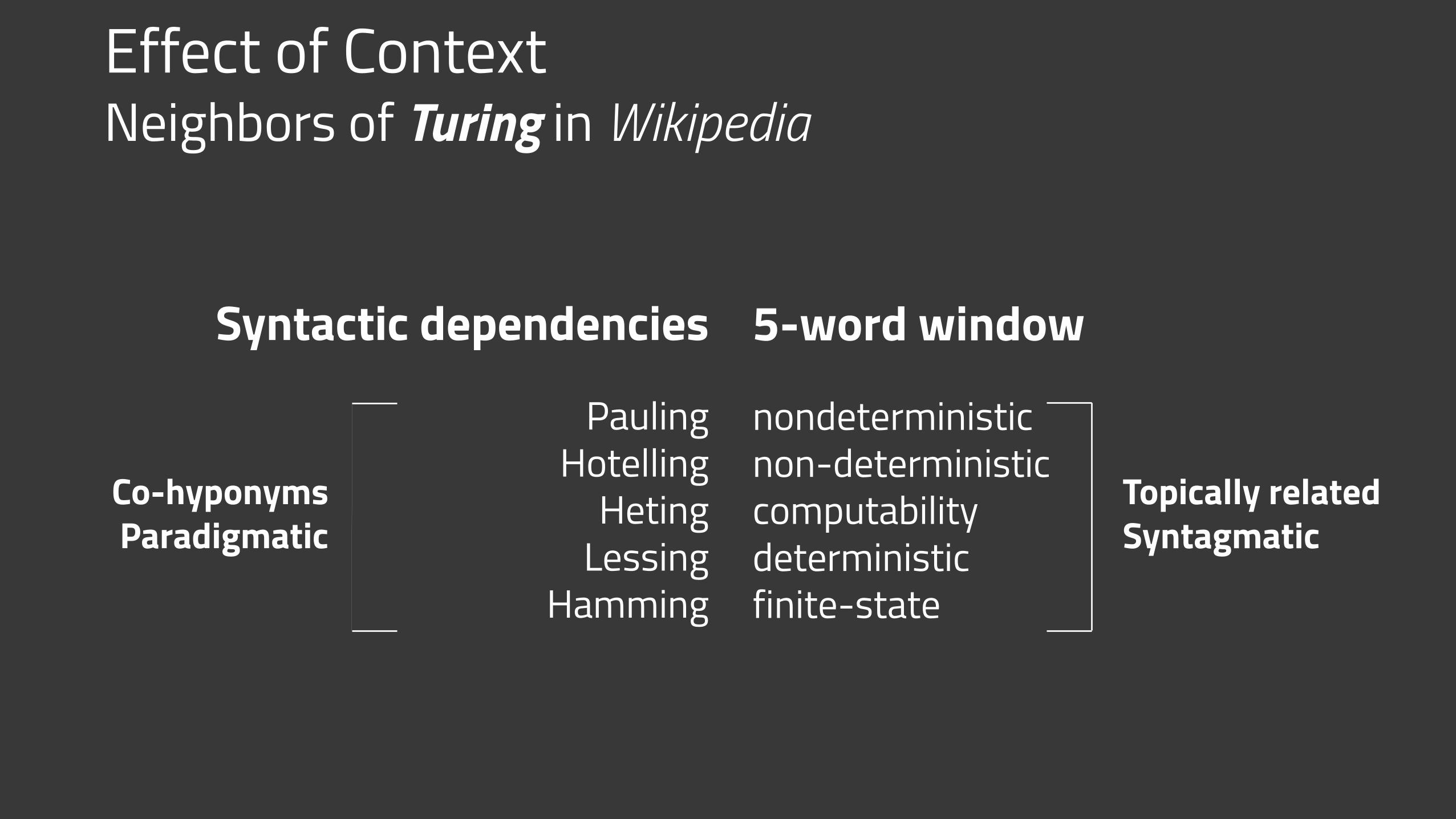
5-word window

nondeterministic non-deterministic computability deterministic finite-state

Syntactic dependencies

Pauling Hotelling

Heting Lessing

Hamming

Effect of Context Neighbors of Turing in Wikipedia

Co-hyponyms Paradigmatic

Topically related Syntagmatic

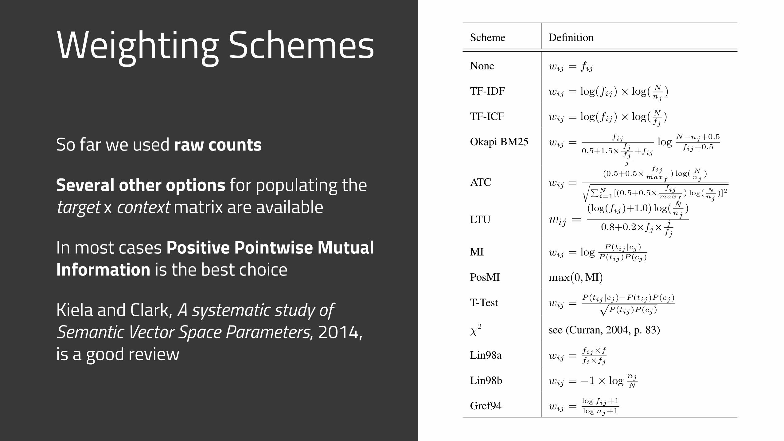
Weighting Schemes

So far we used raw counts

Several other options for populating the target x context matrix are available

In most cases Positive Pointwise Mutual Information is the best choice

Kiela and Clark, A systematic study of Semantic Vector Space Parameters, 2014, is a good review

Measure Definition

Euclidean 1

1+pPn

i=1(ui�vi)2

Cityblock 11+

Pni=1 |ui�vi|

Chebyshev 11+maxi |ui�vi|

Cosine u·v|u||v|

Correlation (u�µu)·(v�µv)|u||v|

Dice 2Pn

i=0 min(ui,vi)Pni=0 ui+vi

Jaccard u·vPni=0 ui+vi

Jaccard2Pn

i=0 min(ui,vi)Pni=0 max(ui,vi)

LinPn

i=0 ui+vi|u|+|v|

Tanimoto u·v|u|+|v|�u·v

Jensen-Shannon Div 1�12 (D(u||u+v

2 )+D(v||u+v2 ))

p2 log 2

↵-skew 1� D(u||↵v+(1�↵)u)p2 log 2

Table 2: Similarity measures between vectors vand u, where vi is the ith component of v

whether removing more context words, based ona frequency cut-off, can improve performance.

3 Experiments

The parameter space is too large to analyse ex-haustively, and so we adopted a strategy for howto navigate through it, selecting certain parame-ters to investigate first, which then get fixed or“clamped” in the remaining experiments. Unlessspecified otherwise, vectors are generated with thefollowing restrictions and transformations on fea-tures: stopwords are removed, numbers mappedto ‘NUM’, and only strings consisting of alphanu-meric characters are allowed. In all experiments,the features consist of the frequency-ranked first nwords in the given source corpus.

Four of the five similarity datasets (RG, MC,W353, MEN) contain continuous scales of sim-ilarity ratings for word pairs; hence we followstandard practice in using a Spearman correlationcoefficient ⇢s for evaluation. The fifth dataset(TOEFL) is a set of multiple-choice questions,for which an accuracy measure is appropriate.Calculating an aggregate score over all datasetsis non-trivial, since taking the mean of correla-tion scores leads to an under-estimation of per-formance; hence for the aggregate score we usethe Fisher-transformed z-variable of the correla-

Scheme Definition

None wij = fij

TF-IDF wij = log(fij)⇥ log( Nnj

)

TF-ICF wij = log(fij)⇥ log(Nfj)

Okapi BM25 wij =fij

0.5+1.5⇥fjfjj

+fijlog

N�nj+0.5

fij+0.5

ATC wij =(0.5+0.5⇥

fijmaxf

) log( Nnj

)rPN

i=1[(0.5+0.5⇥fij

maxf) log( N

nj)]2

LTU wij =(log(fij)+1.0) log( N

nj)

0.8+0.2⇥fj⇥ jfj

MI wij = logP (tij |cj)

P (tij)P (cj)

PosMI max(0,MI)

T-Test wij =P (tij |cj)�P (tij)P (cj)p

P (tij)P (cj)

�2 see (Curran, 2004, p. 83)

Lin98a wij =fij⇥f

fi⇥fj

Lin98b wij = �1⇥ lognj

N

Gref94 wij =log fij+1

lognj+1

Table 3: Term weighting schemes. fij denotes thetarget word frequency in a particular context, fithe total target word frequency, fj the total contextfrequency, N the total of all frequencies, nj thenumber of non-zero contexts. P (tij |cj) is definedas fij

fjand P (tij) as fij

N .

tion datasets, and take the weighted average ofits inverse over the correlation datasets and theTOEFL accuracy score (Silver and Dunlap, 1987).

3.1 Vector size

The first parameter we investigate is vector size,measured by the number of features. Vectors areconstructed from the BNC using a window-basedmethod, with a window size of 5 (2 words eitherside of the target word). We experiment with vec-tor sizes up to 0.5M features, which is close to thetotal number of context words present in the en-tire BNC according to our preprocessing scheme.Features are added according to frequency in theBNC, with increasingly more rare features beingadded. For weighting we consider both PositiveMutual Information and T-Test, which have beenfound to work best in previous research (Bullinariaand Levy, 2012; Curran, 2004). Similarity is com-puted using Cosine.

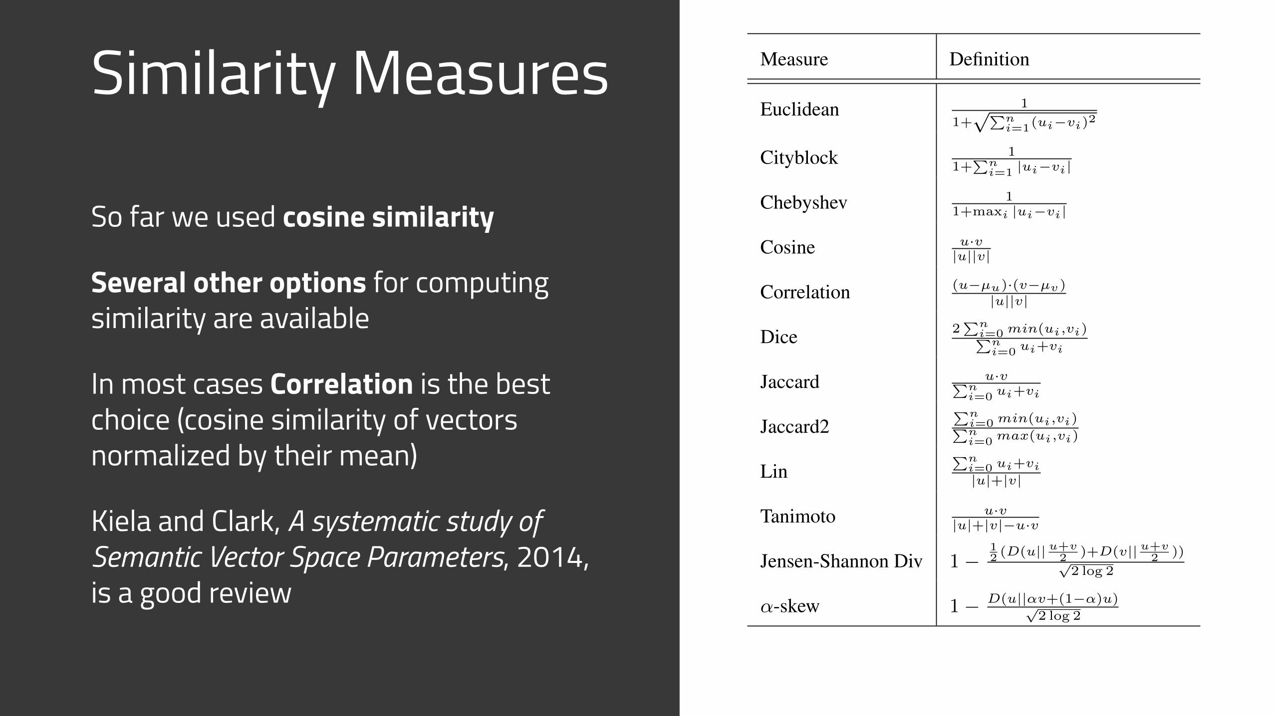
Similarity Measures

So far we used cosine similarity

Several other options for computing similarity are available

In most cases Correlation is the best choice (cosine similarity of vectors normalized by their mean)

Kiela and Clark, A systematic study of Semantic Vector Space Parameters, 2014, is a good review

Measure Definition

Euclidean 1

1+pPn

i=1(ui�vi)2

Cityblock 11+

Pni=1 |ui�vi|

Chebyshev 11+maxi |ui�vi|

Cosine u·v|u||v|

Correlation (u�µu)·(v�µv)|u||v|

Dice 2Pn

i=0 min(ui,vi)Pni=0 ui+vi

Jaccard u·vPni=0 ui+vi

Jaccard2Pn

i=0 min(ui,vi)Pni=0 max(ui,vi)

LinPn

i=0 ui+vi|u|+|v|

Tanimoto u·v|u|+|v|�u·v

Jensen-Shannon Div 1�12 (D(u||u+v

2 )+D(v||u+v2 ))

p2 log 2

↵-skew 1� D(u||↵v+(1�↵)u)p2 log 2

Table 2: Similarity measures between vectors vand u, where vi is the ith component of v

whether removing more context words, based ona frequency cut-off, can improve performance.

3 Experiments

The parameter space is too large to analyse ex-haustively, and so we adopted a strategy for howto navigate through it, selecting certain parame-ters to investigate first, which then get fixed or“clamped” in the remaining experiments. Unlessspecified otherwise, vectors are generated with thefollowing restrictions and transformations on fea-tures: stopwords are removed, numbers mappedto ‘NUM’, and only strings consisting of alphanu-meric characters are allowed. In all experiments,the features consist of the frequency-ranked first nwords in the given source corpus.

Four of the five similarity datasets (RG, MC,W353, MEN) contain continuous scales of sim-ilarity ratings for word pairs; hence we followstandard practice in using a Spearman correlationcoefficient ⇢s for evaluation. The fifth dataset(TOEFL) is a set of multiple-choice questions,for which an accuracy measure is appropriate.Calculating an aggregate score over all datasetsis non-trivial, since taking the mean of correla-tion scores leads to an under-estimation of per-formance; hence for the aggregate score we usethe Fisher-transformed z-variable of the correla-

Scheme Definition

None wij = fij

TF-IDF wij = log(fij)⇥ log( Nnj

)

TF-ICF wij = log(fij)⇥ log(Nfj)

Okapi BM25 wij =fij

0.5+1.5⇥fjfjj

+fijlog

N�nj+0.5

fij+0.5

ATC wij =(0.5+0.5⇥

fijmaxf

) log( Nnj

)rPN

i=1[(0.5+0.5⇥fij

maxf) log( N

nj)]2

LTU wij =(log(fij)+1.0) log( N

nj)

0.8+0.2⇥fj⇥ jfj

MI wij = logP (tij |cj)

P (tij)P (cj)

PosMI max(0,MI)

T-Test wij =P (tij |cj)�P (tij)P (cj)p

P (tij)P (cj)

�2 see (Curran, 2004, p. 83)

Lin98a wij =fij⇥f

fi⇥fj

Lin98b wij = �1⇥ lognj

N

Gref94 wij =log fij+1

lognj+1

Table 3: Term weighting schemes. fij denotes thetarget word frequency in a particular context, fithe total target word frequency, fj the total contextfrequency, N the total of all frequencies, nj thenumber of non-zero contexts. P (tij |cj) is definedas fij

fjand P (tij) as fij

N .

tion datasets, and take the weighted average ofits inverse over the correlation datasets and theTOEFL accuracy score (Silver and Dunlap, 1987).

3.1 Vector size

The first parameter we investigate is vector size,measured by the number of features. Vectors areconstructed from the BNC using a window-basedmethod, with a window size of 5 (2 words eitherside of the target word). We experiment with vec-tor sizes up to 0.5M features, which is close to thetotal number of context words present in the en-tire BNC according to our preprocessing scheme.Features are added according to frequency in theBNC, with increasingly more rare features beingadded. For weighting we consider both PositiveMutual Information and T-Test, which have beenfound to work best in previous research (Bullinariaand Levy, 2012; Curran, 2004). Similarity is com-puted using Cosine.

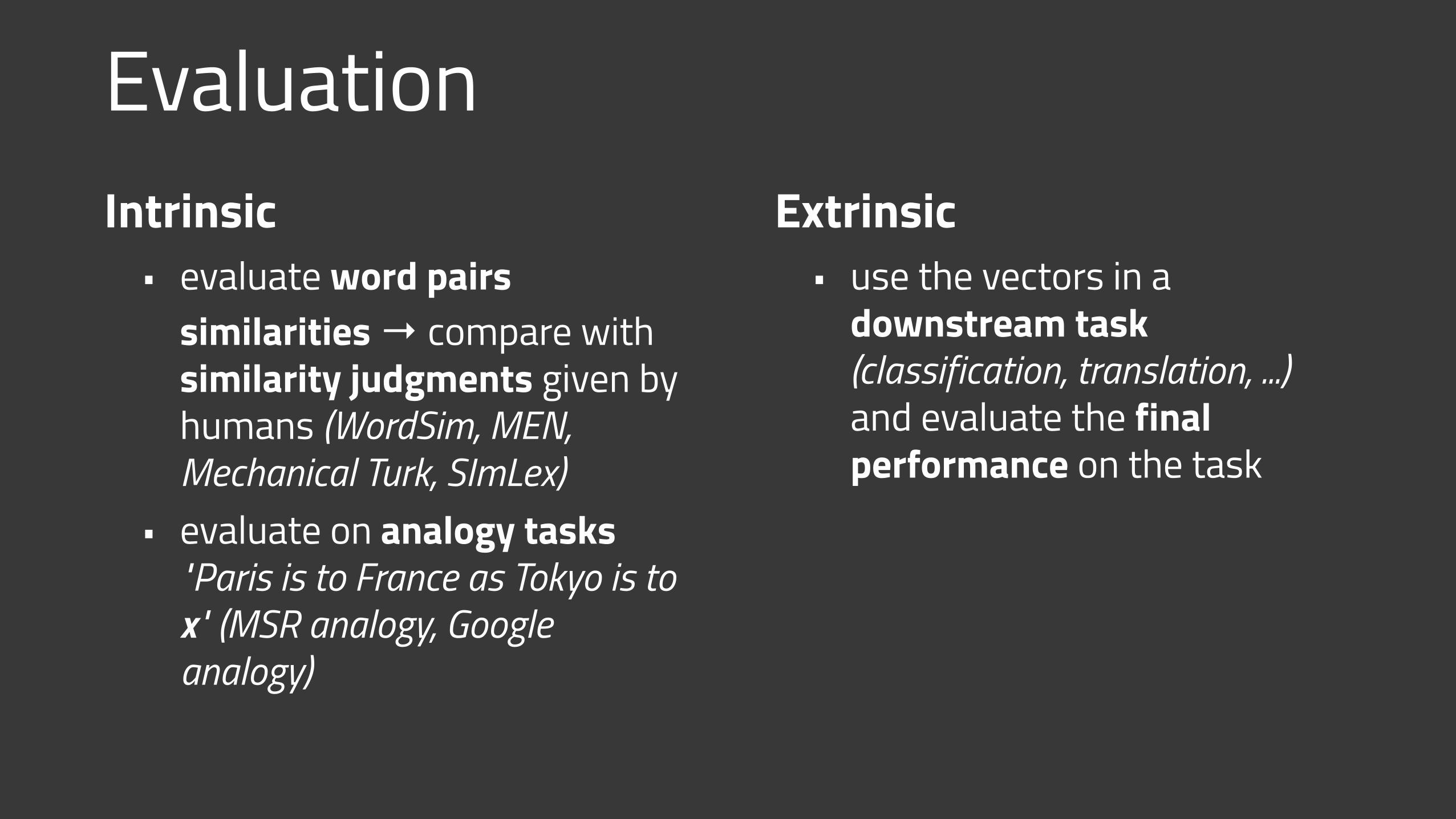
EvaluationIntrinsic

• evaluate word pairs similarities → compare with similarity judgments given by humans (WordSim, MEN, Mechanical Turk, SImLex)

• evaluate on analogy tasks "Paris is to France as Tokyo is to x" (MSR analogy, Google analogy)

Extrinsic • use the vectors in a

downstream task (classification, translation, ...) and evaluate the final performance on the task

Best parameters configuration? (context, similarity measure, weighting, ...)

Depends on the task!

Methods overview

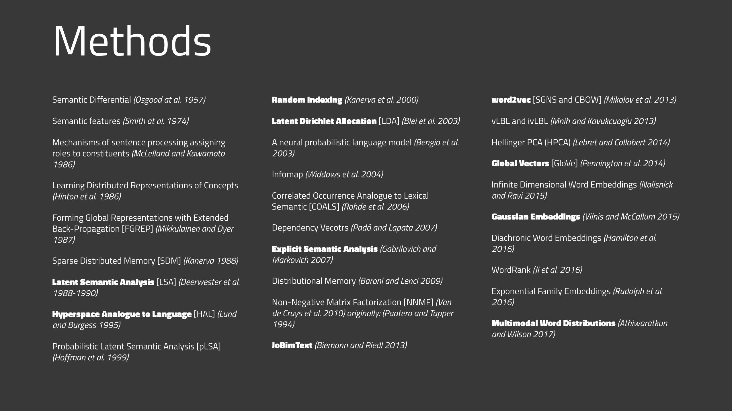
MethodsSemantic Differential (Osgood at al. 1957)

Semantic features (Smith at al. 1974)

Mechanisms of sentence processing assigning roles to constituents (McLelland and Kawamoto 1986)

Learning Distributed Representations of Concepts (Hinton et al. 1986)

Forming Global Representations with Extended Back-Propagation [FGREP] (Mikkulainen and Dyer 1987)

Sparse Distributed Memory [SDM] (Kanerva 1988)

Latent Semantic Analysis [LSA] (Deerwester et al.1988-1990)

Hyperspace Analogue to Language [HAL] (Lund and Burgess 1995)

Probabilistic Latent Semantic Analysis [pLSA] (Hoffman et al. 1999)

Random Indexing (Kanerva et al. 2000)

Latent Dirichlet Allocation [LDA] (Blei et al. 2003)

A neural probabilistic language model (Bengio et al. 2003)

Infomap (Widdows et al. 2004)

Correlated Occurrence Analogue to Lexical Semantic [COALS] (Rohde et al. 2006)

Dependency Vecotrs (Padó and Lapata 2007)

Explicit Semantic Analysis (Gabrilovich and Markovich 2007)

Distributional Memory (Baroni and Lenci 2009)

Non-Negative Matrix Factorization [NNMF] (Van de Cruys et al. 2010) originally: (Paatero and Tapper 1994)

JoBimText (Biemann and Riedl 2013)

word2vec [SGNS and CBOW] (Mikolov et al. 2013)

vLBL and ivLBL (Mnih and Kavukcuoglu 2013)

Hellinger PCA (HPCA) (Lebret and Collobert 2014)

Global Vectors [GloVe] (Pennington et al. 2014)

Infinite Dimensional Word Embeddings (Nalisnick and Ravi 2015)

Gaussian Embeddings (Vilnis and McCallum 2015)

Diachronic Word Embeddings (Hamilton et al. 2016)

WordRank (Ji et al. 2016)

Exponential Family Embeddings (Rudolph et al. 2016)

Multimodal Word Distributions (Athiwaratkun and Wilson 2017)

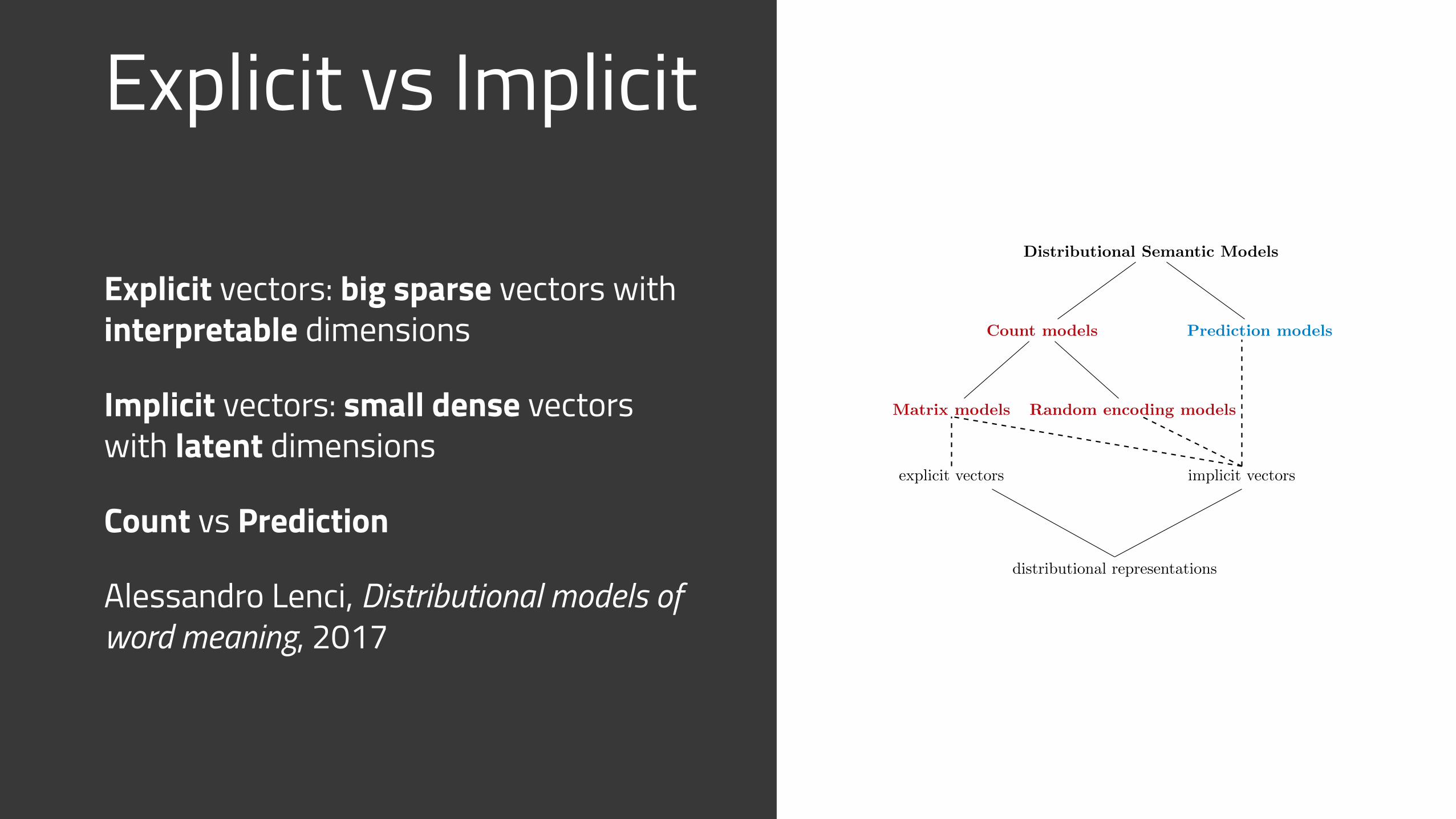
Explicit vs Implicit

Explicit vectors: big sparse vectors with interpretable dimensions

Implicit vectors: small dense vectors with latent dimensions

Count vs Prediction

Alessandro Lenci, Distributional models of word meaning, 2017

Distributional Semantic Models

Count models

Matrix models Random encoding models

Prediction models

distributional representations

explicit vectors implicit vectors

Distributional Semantic Models

Word models(lexemes)

Window-based models(window-based collocates)

Syntactic models(syntactic collocates)

Region models(text regions)

Figure 2

A classification of DSMs based on (left) context types and (right) methods to build distributional vectors

Table 2 Most common matrix DSMs.

Model name Description

Latent Semantic Analysis (LSA)a word-by-region matrix, weighted with entropy and reduced with SVD

Hyperspace Analogue of Language (HAL)b window-based model with directed collocates

Dependency Vectors (DV)c syntactic model with dependency-filtered collocates

Latent Relational Analysis (LRA)d pair-by-pattern matrix reduced with SVD to measure relational similarity

Distributional Memory (DM)e target–link–context tuples formalized with a high-order tensor

Topic Modelsf word-by-region matrix reduced with Bayesian inference

High Dimensional Explorer (HiDEx)g generalization of HAL with a larger range of parameter settings

Global Vectors (GloVe)h word-by-word matrix reduced with weighted least squares regression

aLandauer & Dumais (1997); bBurgess (1998); cPado & Lapata (2007); dTurney (2006); eBaroni & Lenci

(2010); fGri�ths et al. (2007); gShaoul & Westbury (2010); hPennington et al. (2014).

shown that narrow context windows and syntactic collocates are best to capture lexemes

related by paradigmatic semantic relations (e.g., synonyms and antonyms) or belonging to

the same taxonomic category (e.g., violin and guitar), because they share very close collo-

cates (Sahlgren 2006; Bullinaria & Levy 2007; Van de Cruys 2008; Baroni & Lenci 2011;

Bullinaria & Levy 2012; Kiela & Clark 2014; Levy & Goldberg 2014a). Conversely, collo-

cates extracted with larger context windows are biased towards more associative semantic

relations (e.g., violin and music), like region models.

The second dimension of variation among DSMs is the method to learn distributional

representations. Matrix models (see Table 2) are a rich family of DSMs that generalize the

vector space model in information retrieval (see Section 2). They are a subtype of so-called

count models (Baroni et al. 2014b), which learn the representation of a target lexeme by

recording and counting its co-occurrences in linguistic contexts. Matrix models arrange

distributional data into co-occurrence matrices. The matrix is a formal representation of

the global distributional statistics extracted from the corpus. The weighting functions use

such global statistics to estimate the importance of co-occurrences to characterize target

www.annualreviews.org • Distributional semantics 9

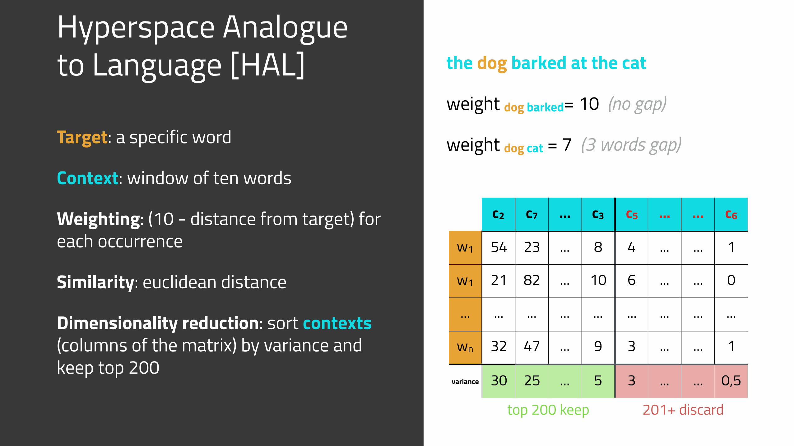
Hyperspace Analogue to Language [HAL]

Target: a specific word

Context: window of ten words

Weighting: (10 - distance from target) for each occurrence

Similarity: euclidean distance

Dimensionality reduction: sort contexts (columns of the matrix) by variance and keep top 200

the dog barked at the cat

weight dog barked= 10 (no gap)

weight dog cat = 7 (3 words gap)

c2 c7 ... c3 c5 ... ... c6

w1 54 23 ... 8 4 ... ... 1

w1 21 82 ... 10 6 ... ... 0

... ... ... ... ... ... ... ... ...

wn 32 47 ... 9 3 ... ... 1

variance 30 25 ... 5 3 ... ... 0,5

201+ discardtop 200 keep

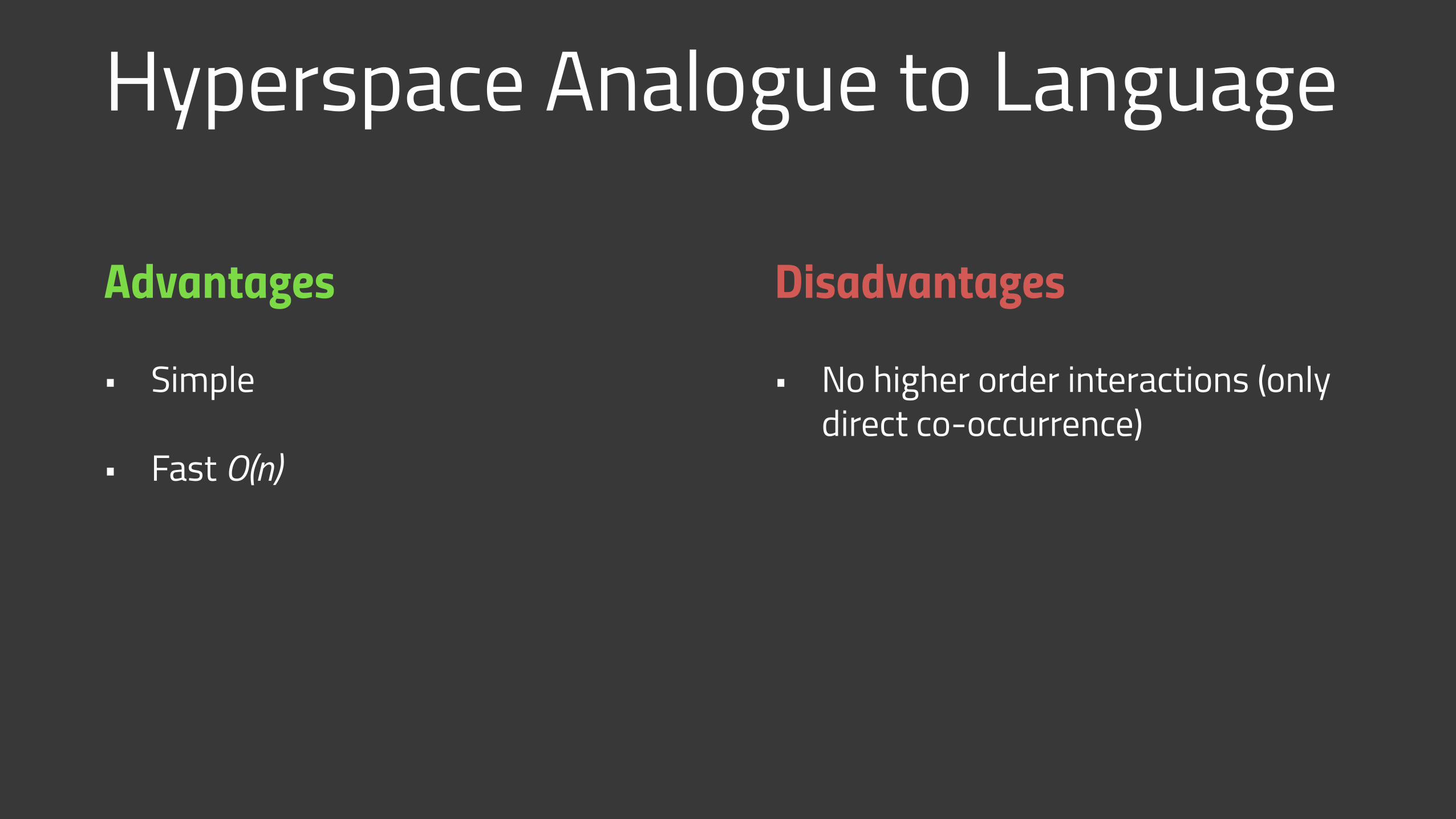
Hyperspace Analogue to Language

Advantages

• Simple

• Fast O(n)

Disadvantages

• No higher order interactions (only direct co-occurrence)

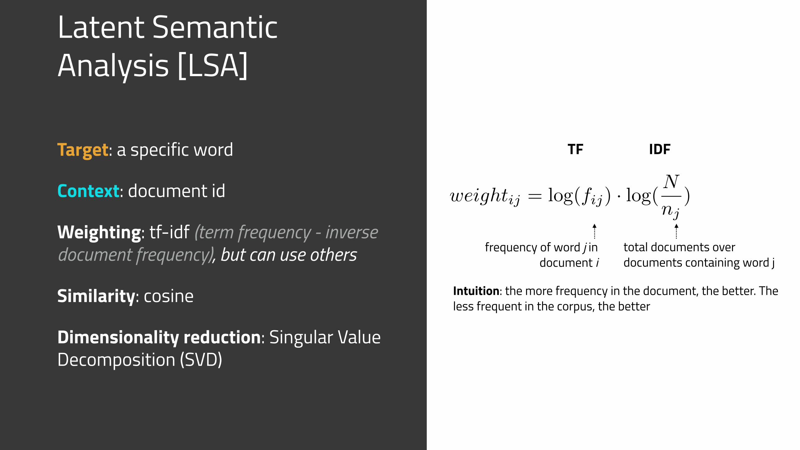
Latent Semantic Analysis [LSA]


Context: document id

Weighting: tf-idf (term frequency - inverse document frequency), but can use others

Similarity: cosine

Dimensionality reduction: Singular Value Decomposition (SVD)

weightij = log(fij) · log(N

nj)

frequency of word j in document i

total documents over documents containing word j

Intuition: the more frequency in the document, the better. The less frequent in the corpus, the better

TF IDF

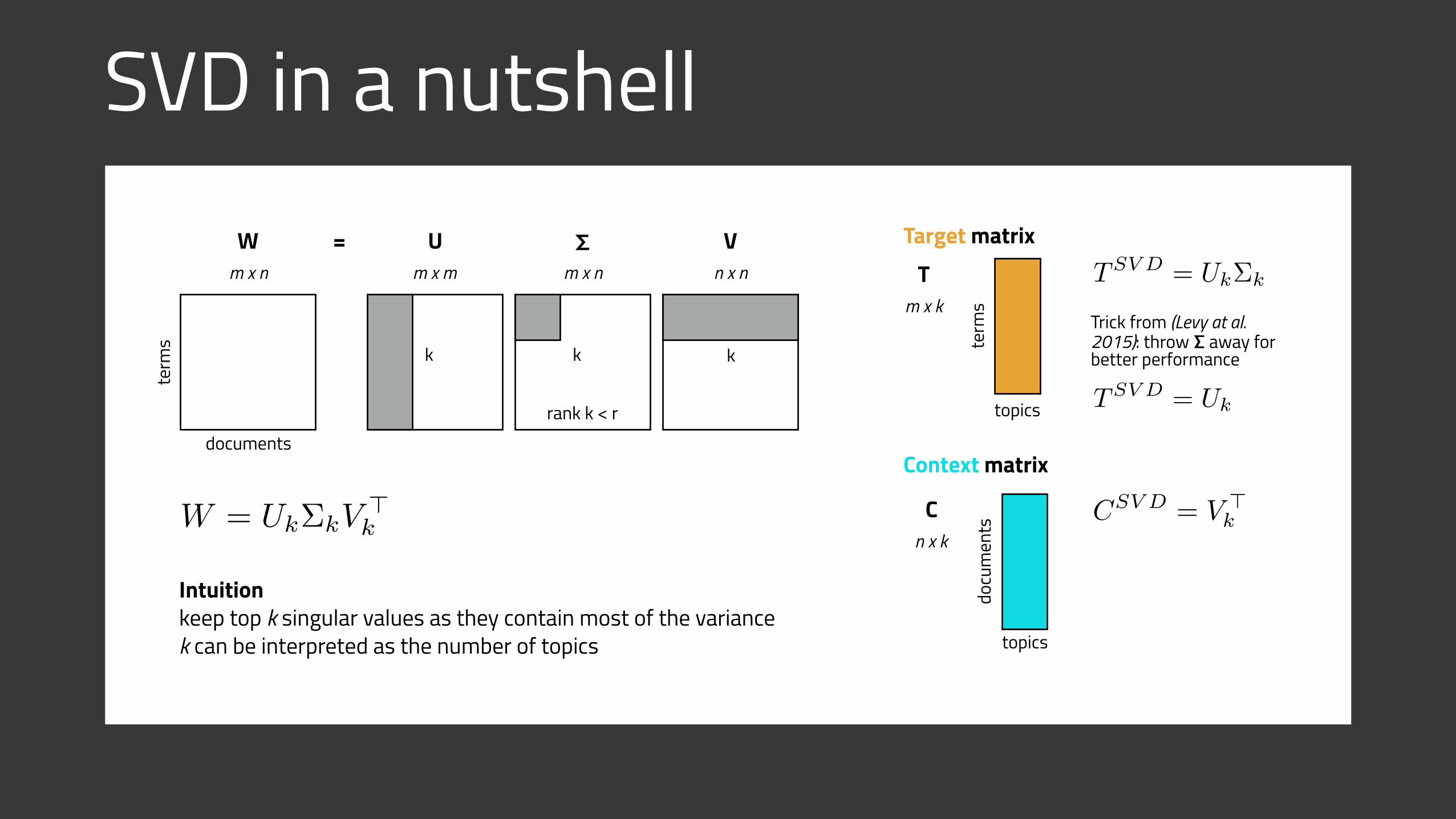
SVD in a nutshell

documents

term

s

Wm x n

Um x m

𝝨m x n

Vn x n

=

rank k < r

kk k

Intuition keep top k singular values as they contain most of the variance k can be interpreted as the number of topics

W = Uk⌃kV>k

Target matrixTSV D = Uk⌃k

TSV D = Uk

Context matrix

Trick from (Levy at al. 2015): throw 𝝨 away for better performance

Cn x k

topics

docu

men

ts

Tm x k

topics

term

s

CSV D = V >k

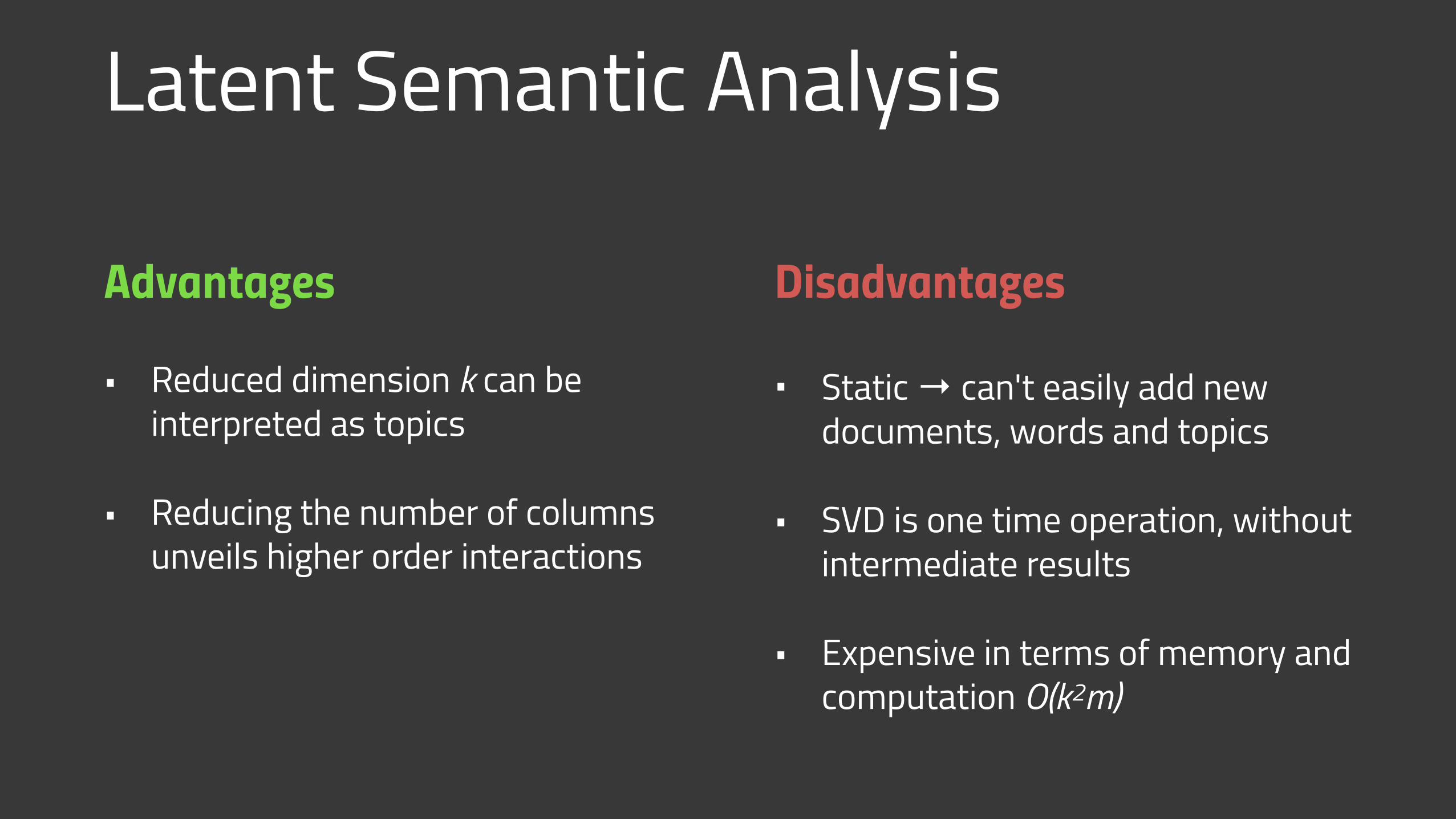
Latent Semantic Analysis

Advantages

• Reduced dimension k can be interpreted as topics

• Reducing the number of columns unveils higher order interactions

Disadvantages

• Static → can't easily add new documents, words and topics

• SVD is one time operation, without intermediate results

• Expensive in terms of memory and computation O(k2m)

Random Indexing [RI]

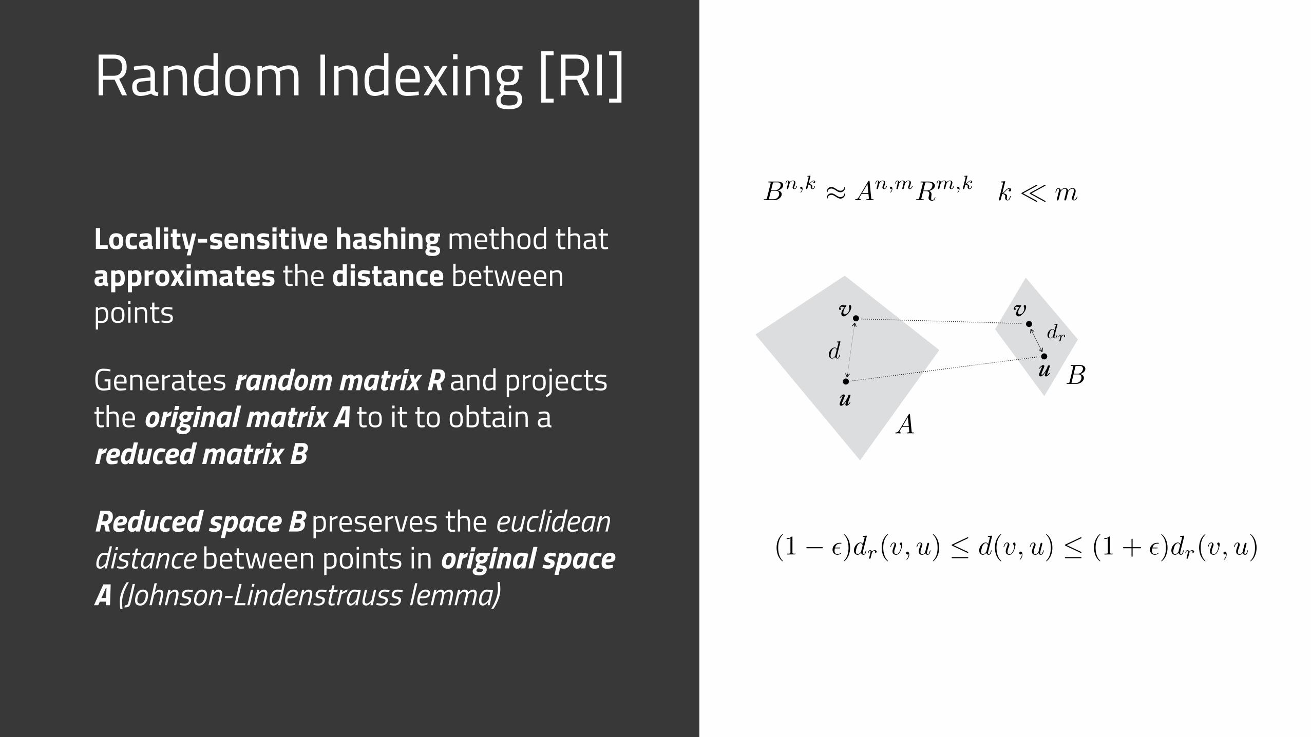
Locality-sensitive hashing method that approximates the distance between points

Generates random matrix R and projects the original matrix A to it to obtain a reduced matrix B

Reduced space B preserves the euclidean distance between points in original space A (Johnson-Lindenstrauss lemma)

Bn,k ⇡ An,mRm,k k ⌧ m

(1� ✏)dr(v, u) d(v, u) (1 + ✏)dr(v, u)

A

Bd

dr

uu

v v

Random Indexing [RI]

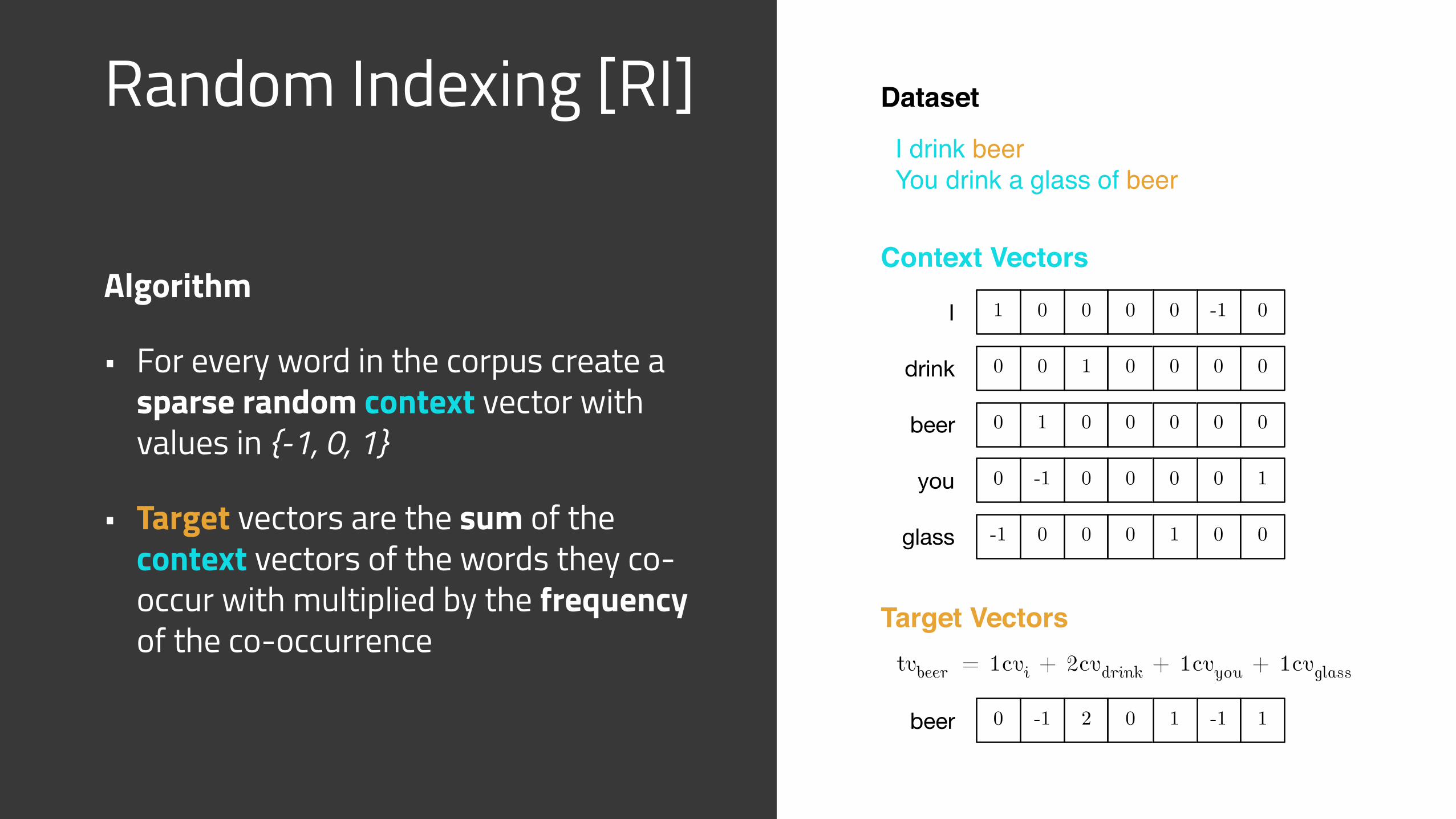
Algorithm

• For every word in the corpus create a sparse random context vector with values in {-1, 0, 1}

• Target vectors are the sum of the context vectors of the words they co-occur with multiplied by the frequency of the co-occurrence

1 0I 0 0 0 -1 0

drink 0 0 1 0 0 0 0

I drink beerYou drink a glass of beer

Dataset

Context Vectors

beer 0 1 0 0 0 0 0

you 0 -1 0 0 0 0 1

glass -1 0 0 0 1 0 0

tvbeer = 1cvi + 2cvdrink + 1cvyou + 1cvglass

Term Vectors

beer 0 -1 2 0 1 -1 1

Context Vectors

Target Vectors

Dataset

I drink beerYou drink a glass of beer

Random Indexing

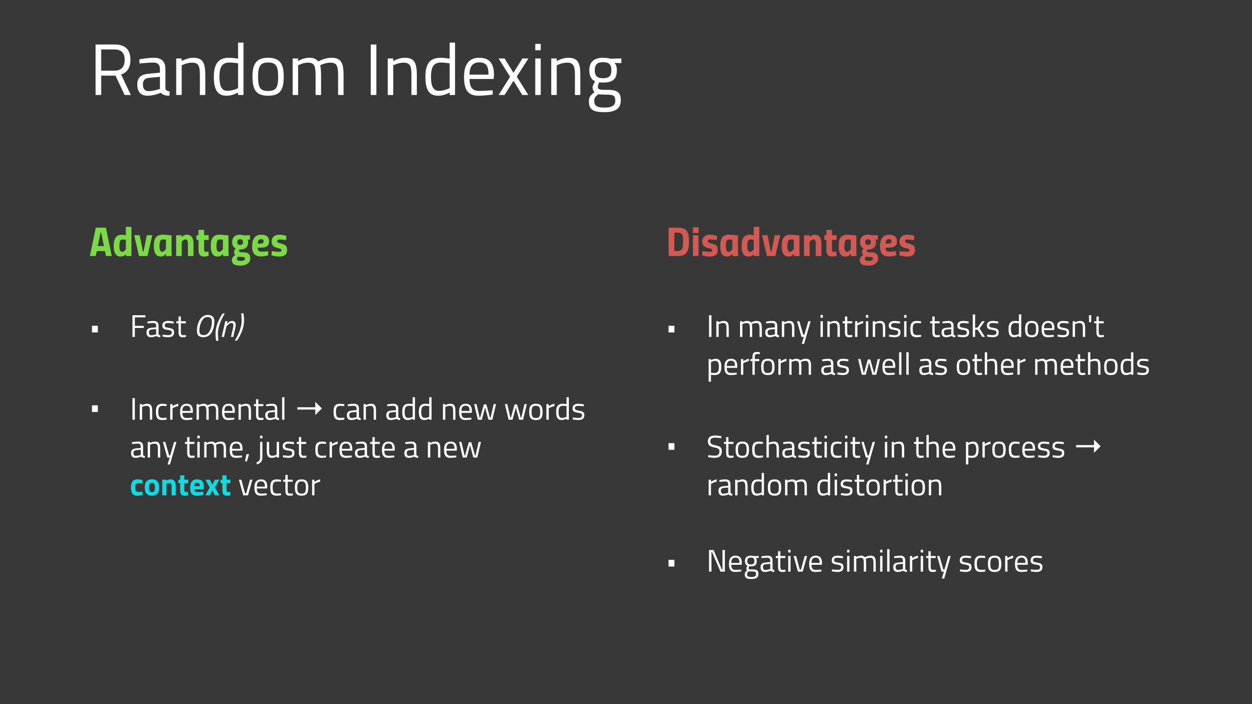
Advantages

• Fast O(n)

• Incremental → can add new words any time, just create a new context vector

Disadvantages

• In many intrinsic tasks doesn't perform as well as other methods

• Stochasticity in the process → random distortion

• Negative similarity scores

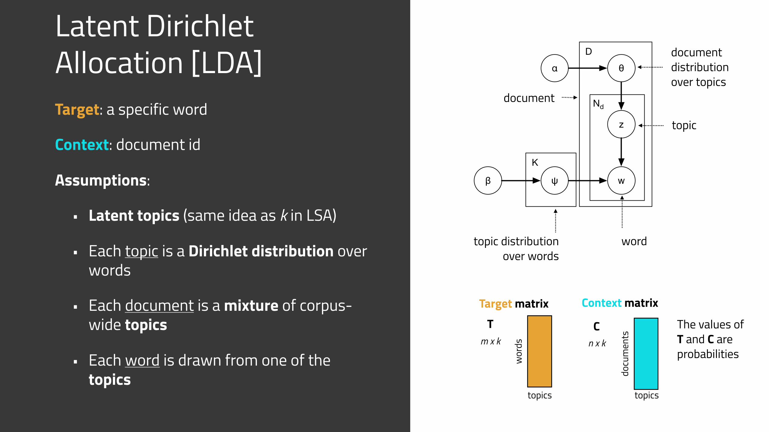
Latent Dirichlet Allocation [LDA]Target: a specific word

Context: document id

Assumptions:

• Latent topics (same idea as k in LSA)

• Each topic is a Dirichlet distribution over words

• Each document is a mixture of corpus-wide topics

• Each word is drawn from one of the topics

α θ

z

wψβ

K

D

Nd

topic distribution over words

word

topic

document distribution over topics

document

Target matrix Context matrix

Cn x k

docu

men

ts

Tm x k

topics

wor

ds

topics

The values of T and C are probabilities

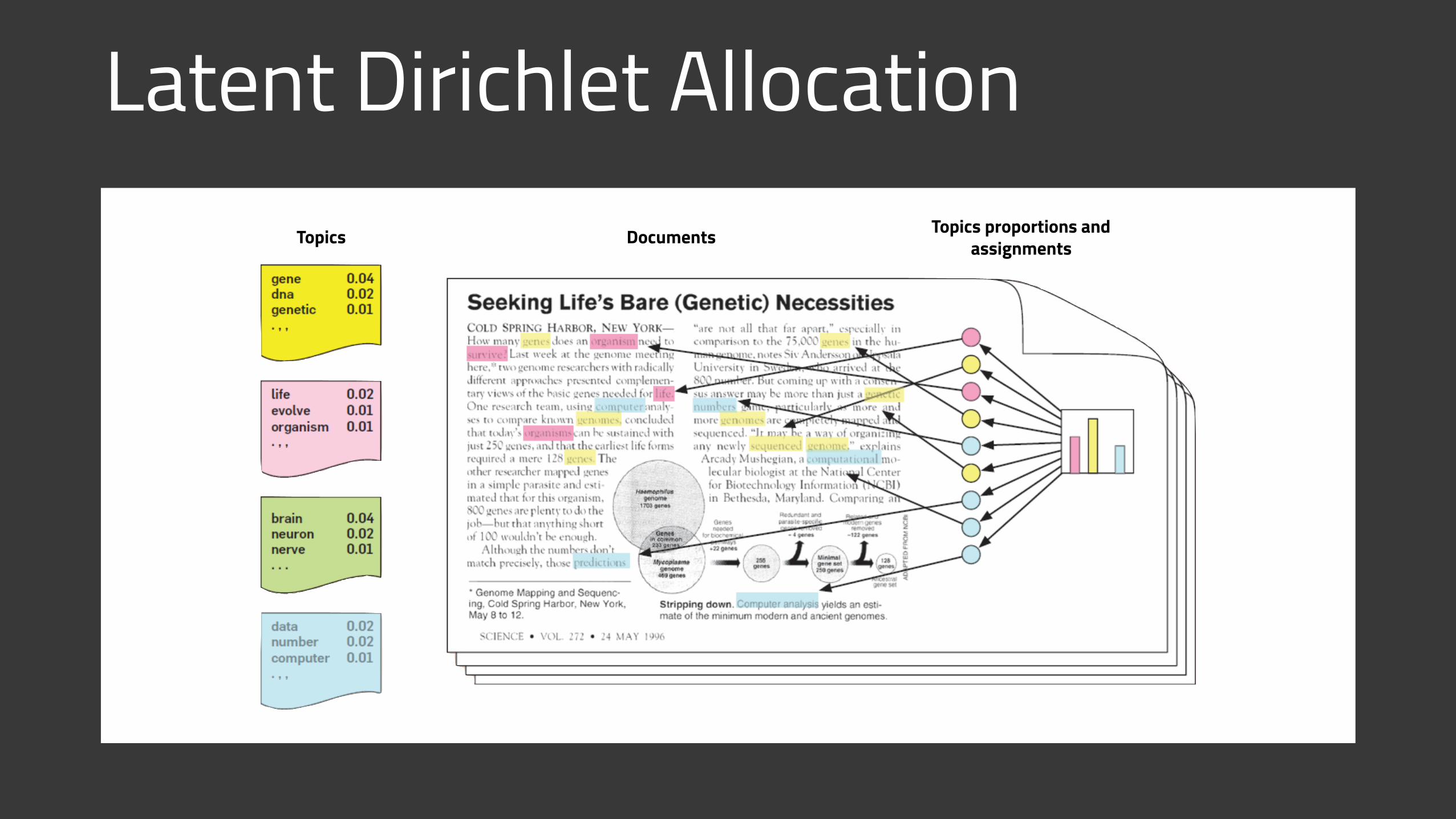
Latent Dirichlet AllocationDocumentsTopics Topics proportions and

assignments

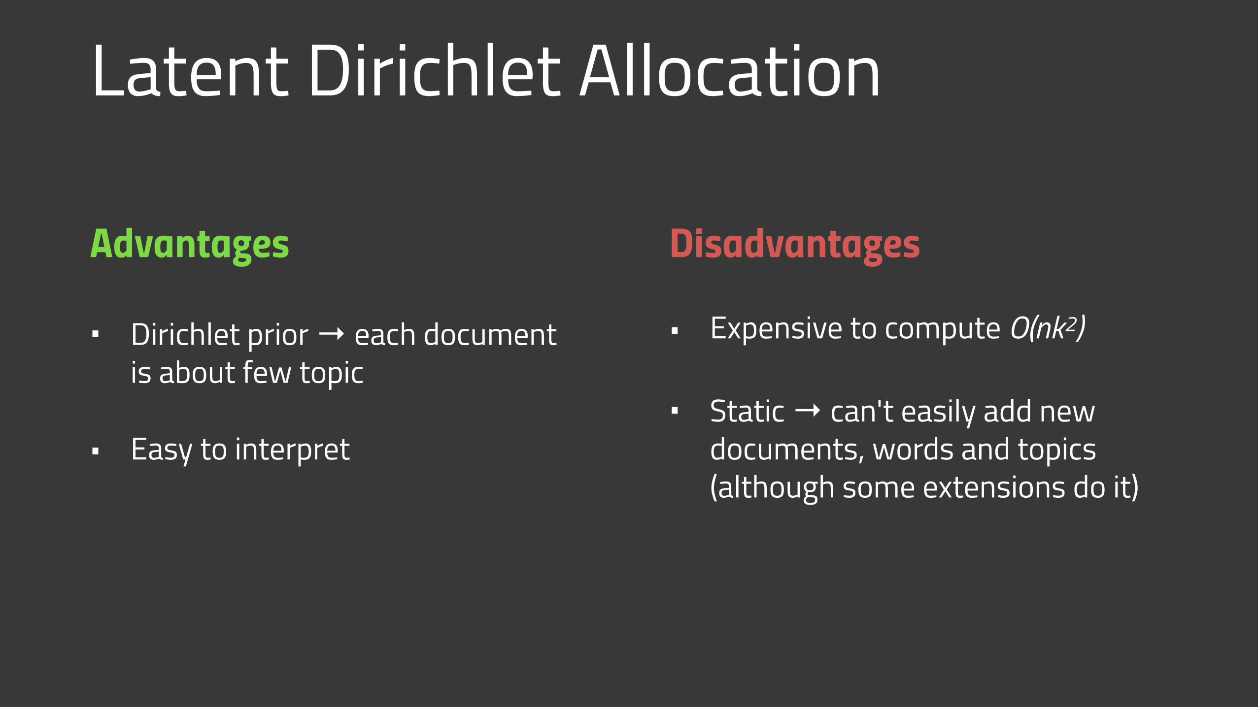
Latent Dirichlet Allocation

Advantages

• Dirichlet prior → each document is about few topic

• Easy to interpret

Disadvantages

• Expensive to compute O(nk2)

• Static → can't easily add new documents, words and topics (although some extensions do it)

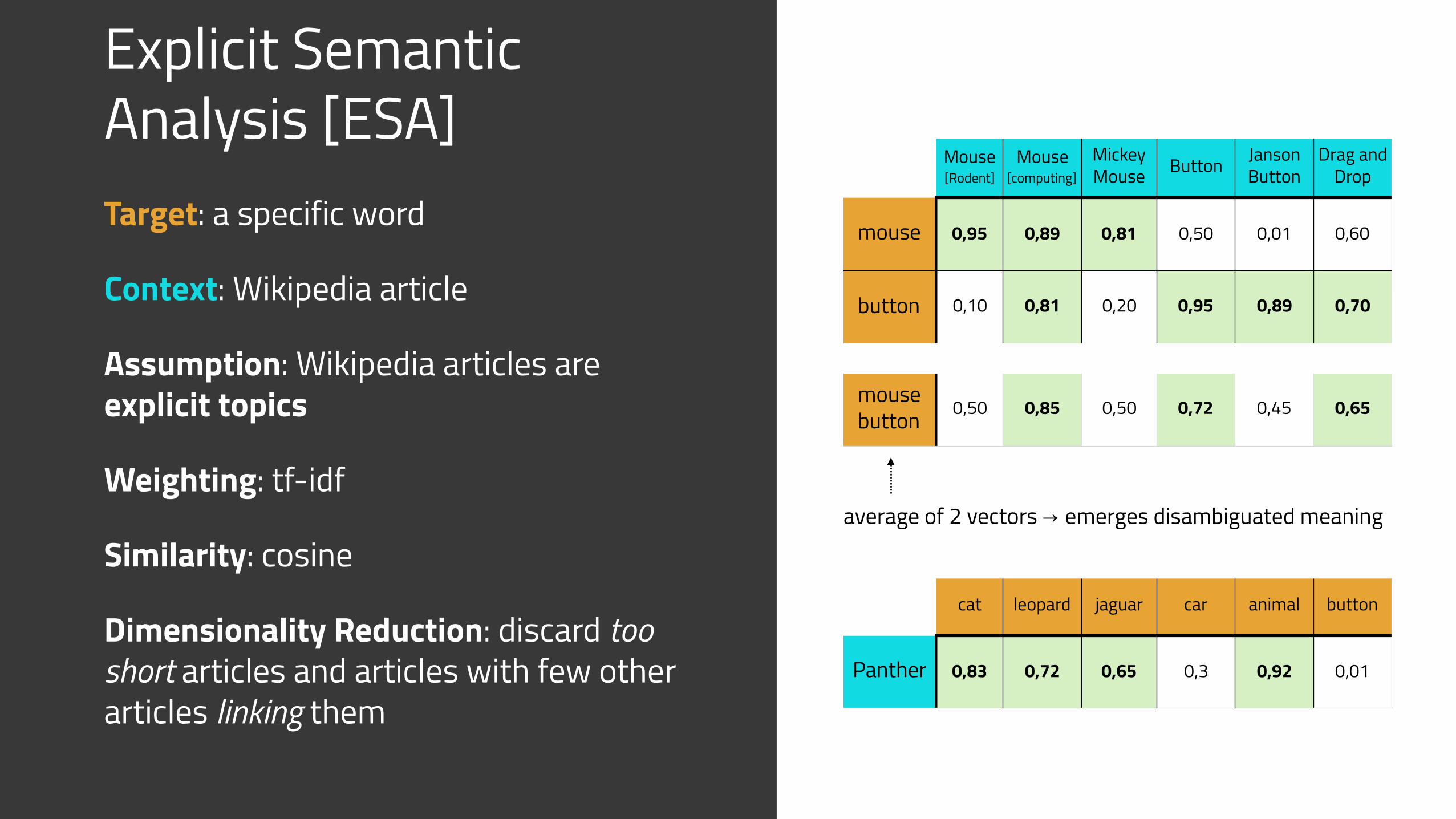
Explicit Semantic Analysis [ESA]Target: a specific word

Context: Wikipedia article

Assumption: Wikipedia articles are explicit topics

Weighting: tf-idf

Similarity: cosine

Dimensionality Reduction: discard too short articles and articles with few other articles linking them

Mouse [Rodent]

Mouse [computing]

Mickey Mouse Button Janson

ButtonDrag and

Drop

mouse 0,95 0,89 0,81 0,50 0,01 0,60

button 0,10 0,81 0,20 0,95 0,89 0,70

mouse button 0,50 0,85 0,50 0,72 0,45 0,65

average of 2 vectors → emerges disambiguated meaning

cat leopard jaguar car animal button

Panther 0,83 0,72 0,65 0,3 0,92 0,01

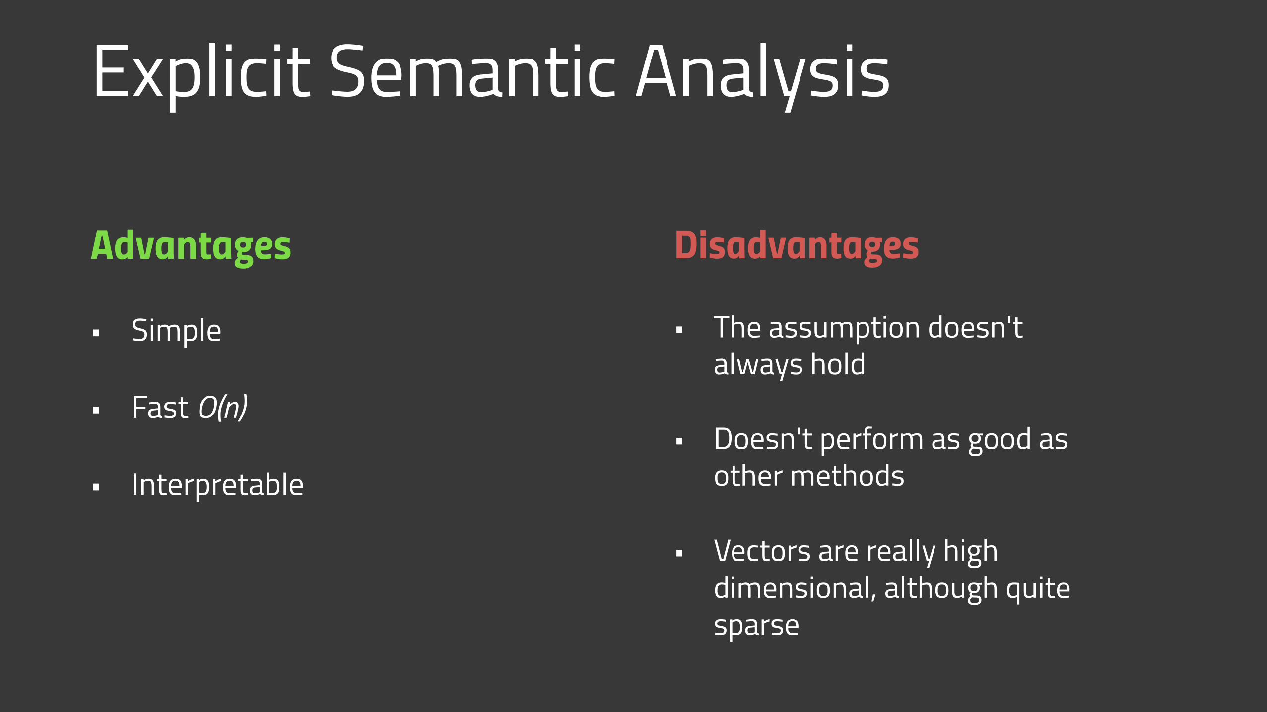
Explicit Semantic Analysis

Advantages

• Simple

• Fast O(n)

• Interpretable

Disadvantages

• The assumption doesn't always hold

• Doesn't perform as good as other methods

• Vectors are really high dimensional, although quite sparse

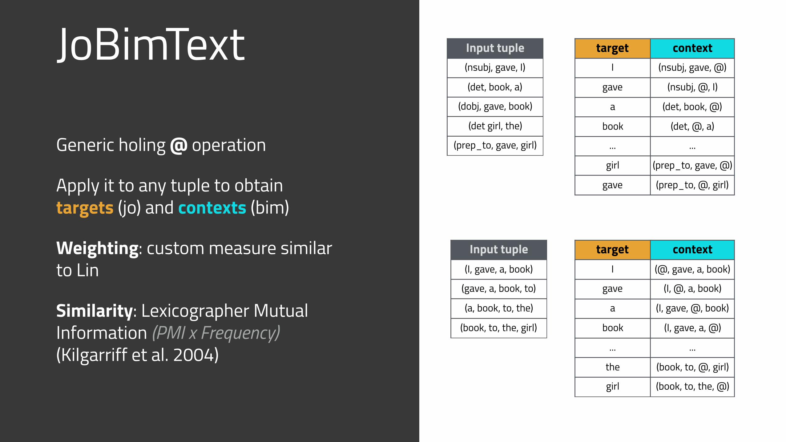
JoBimText

Generic holing @ operation

Apply it to any tuple to obtain targets (jo) and contexts (bim)

Weighting: custom measure similar to Lin

Similarity: Lexicographer Mutual Information (PMI x Frequency) (Kilgarriff et al. 2004)

target contextI (nsubj, gave, @)

gave (nsubj, @, I)

a (det, book, @)

book (det, @, a)

... ...

girl (prep_to, gave, @)

gave (prep_to, @, girl)

Input tuple(nsubj, gave, I)

(det, book, a)

(dobj, gave, book)

(det girl, the)

(prep_to, gave, girl)

target contextI (@, gave, a, book)

gave (I, @, a, book)

a (I, gave, @, book)

book (I, gave, a, @)

... ...

the (book, to, @, girl)

girl (book, to, the, @)

Input tuple(I, gave, a, book)

(gave, a, book, to)

(a, book, to, the)

(book, to, the, girl)

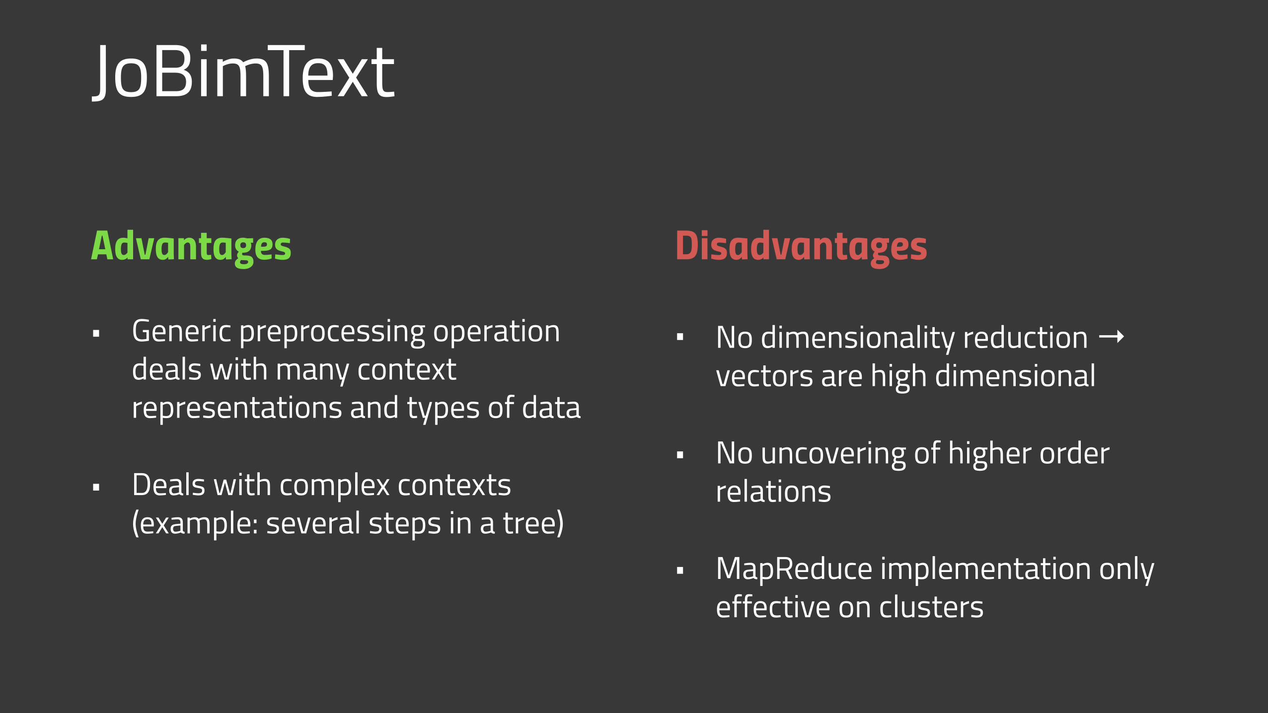
JoBimText

Advantages

• Generic preprocessing operation deals with many context representations and types of data

• Deals with complex contexts (example: several steps in a tree)

Disadvantages

• No dimensionality reduction → vectors are high dimensional

• No uncovering of higher order relations

• MapReduce implementation only effective on clusters

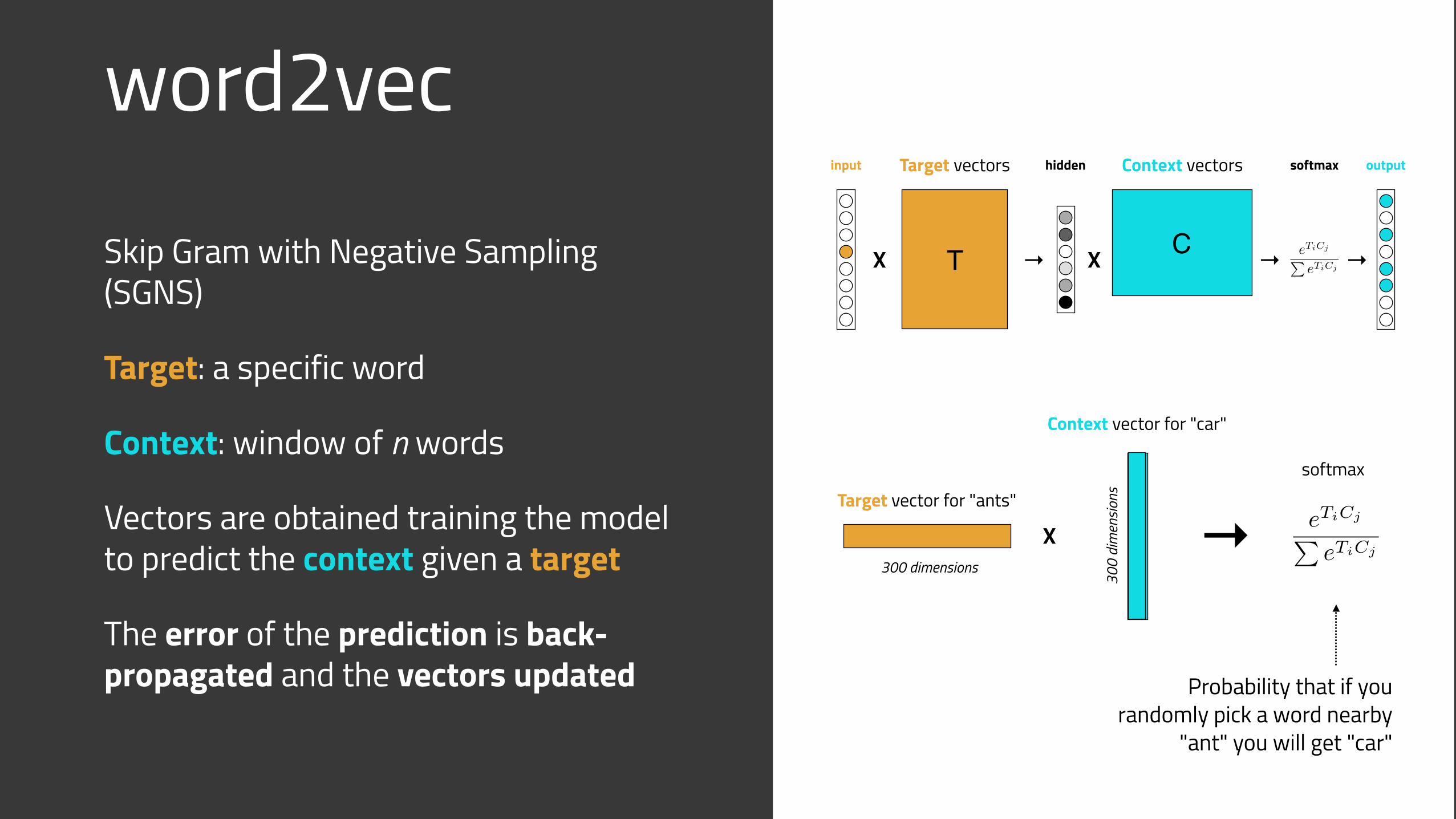
word2vec

Skip Gram with Negative Sampling (SGNS)


Context: window of n words

Vectors are obtained training the model to predict the context given a target

The error of the prediction is back-propagated and the vectors updated Probability that if you

randomly pick a word nearby "ant" you will get "car"

eTiCj

PeTiCj

X T X C

Target vectors Context vectorsinput

→

output

→→

hidden softmax

300 dimensions

300

dim

ensio

ns

X →Target vector for "ants"

Context vector for "car"

eTiCj

PeTiCj

softmax

Example

X

The quick brown fox jumps over the lazy dog

T XC

Target vectors Context vectors

the

one hot

softmax→brown

fox

quickjumps

over

doglazy

the

brownfox

quickjumps

over

doglazy

prediction

the

brownfox

quickjumps

over

doglazy

ground truth

They should be the same

→→

hidden

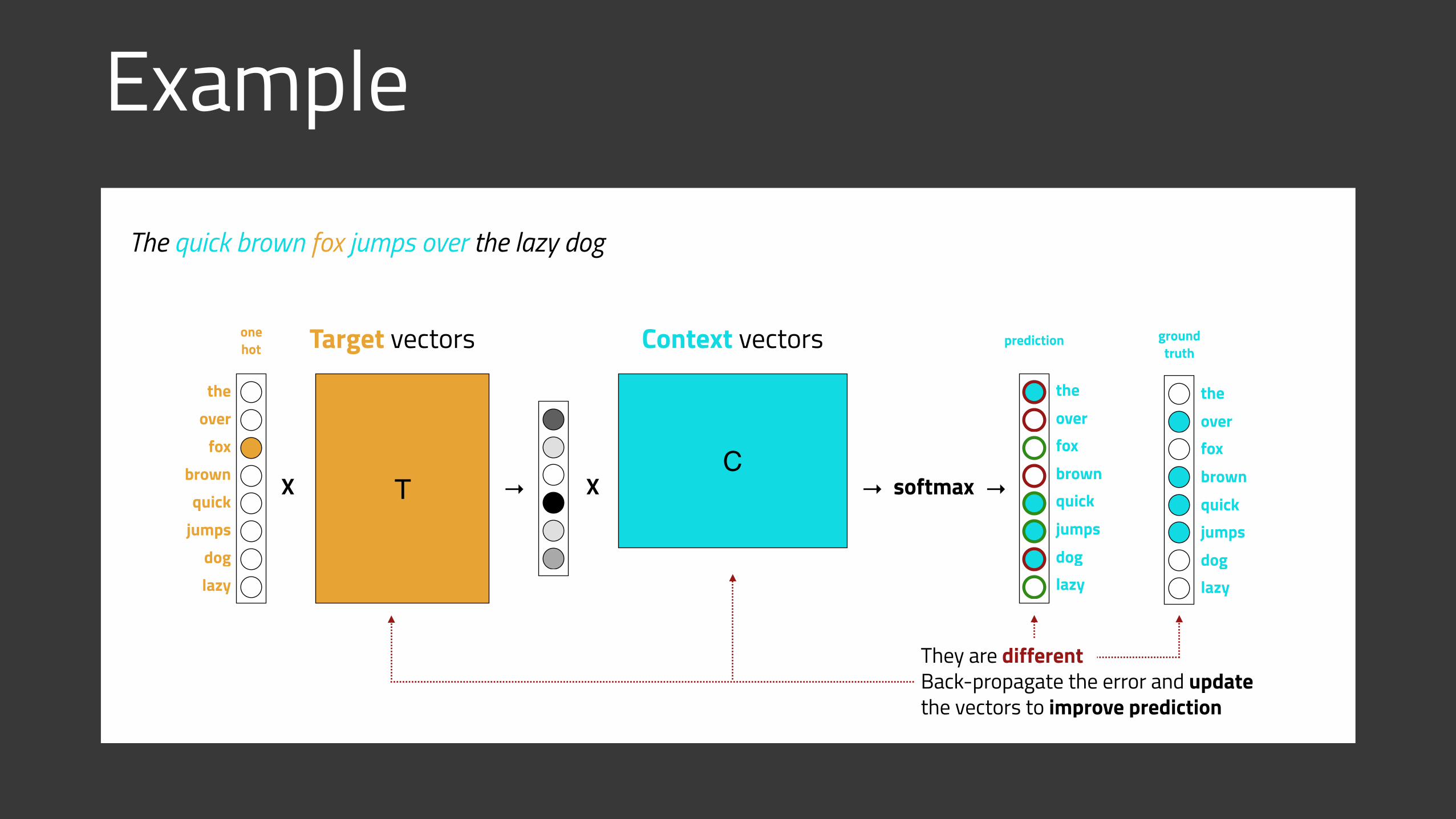
Example

X


T XC


the

one hot

softmax→brown

fox

quickjumps

over

doglazy

the

brownfox

quickjumps

over

doglazy

prediction

the

brownfox

quickjumps

over

doglazy

ground truth

They are different Back-propagate the error and update the vectors to improve prediction

→ →

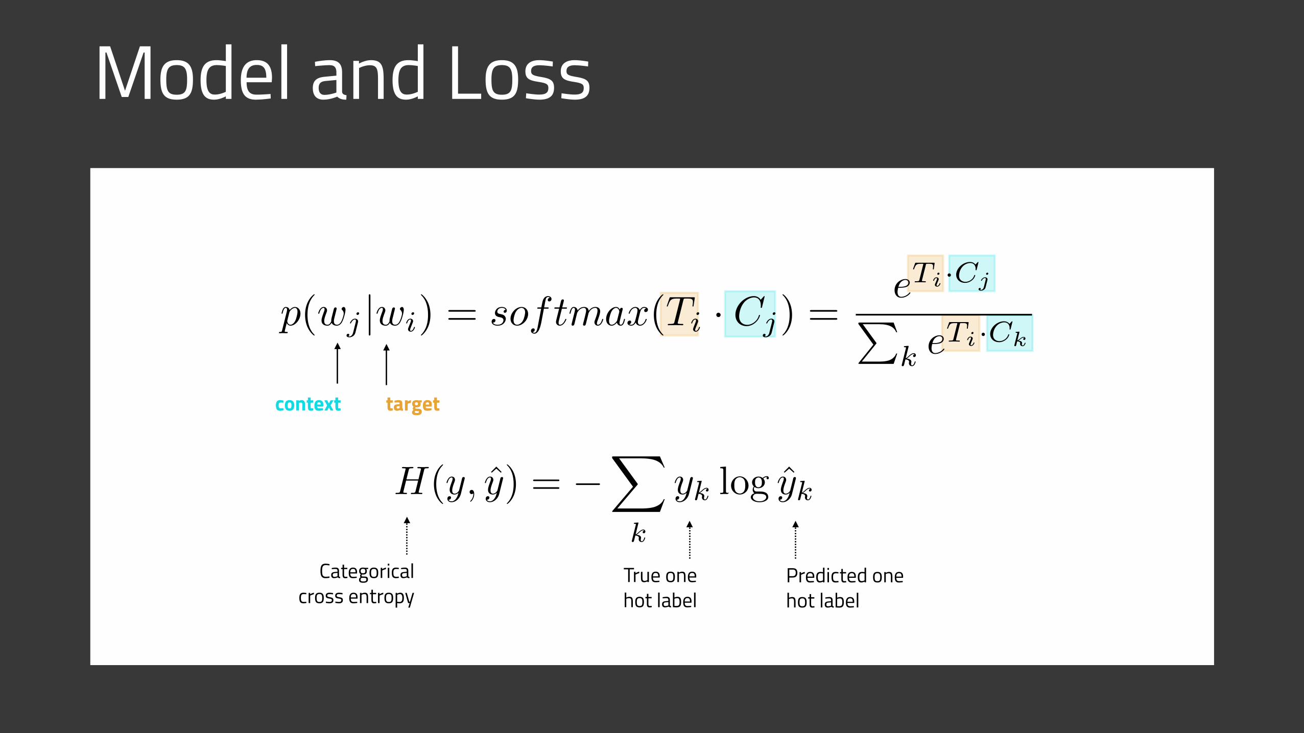
Model and Loss

H(y, y) = �X

k

yk log yk

Categorical cross entropy

True one hot label

Predicted one hot label

targetcontext

p(wj |wi) = softmax(Ti · Cj) =eTi·Cj

Pk e

Ti·Ck

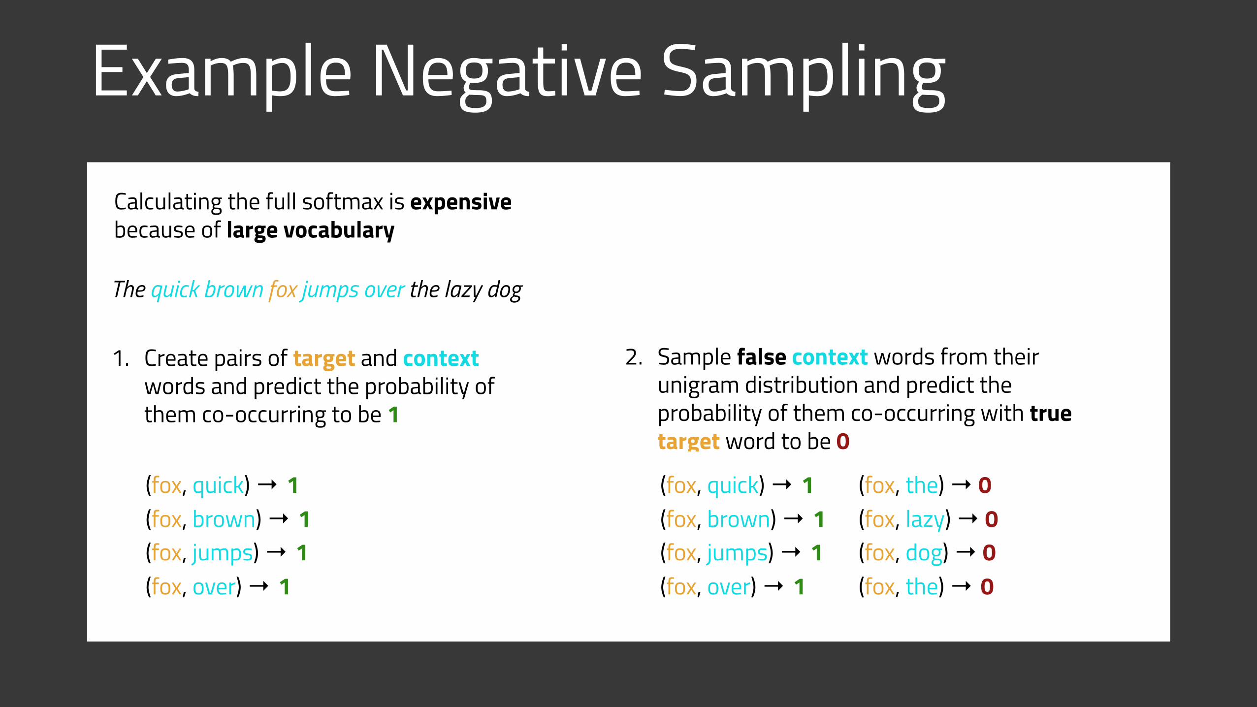
Example Negative Sampling


Calculating the full softmax is expensive because of large vocabulary

1. Create pairs of target and context words and predict the probability of them co-occurring to be 1

2. Sample false context words from their unigram distribution and predict the probability of them co-occurring with true target word to be 0

(fox, quick) → 1 (fox, brown) → 1 (fox, jumps) → 1 (fox, over) → 1

(fox, quick) → 1 (fox, brown) → 1 (fox, jumps) → 1 (fox, over) → 1

(fox, the) → 0 (fox, lazy) → 0 (fox, dog) → 0 (fox, the) → 0

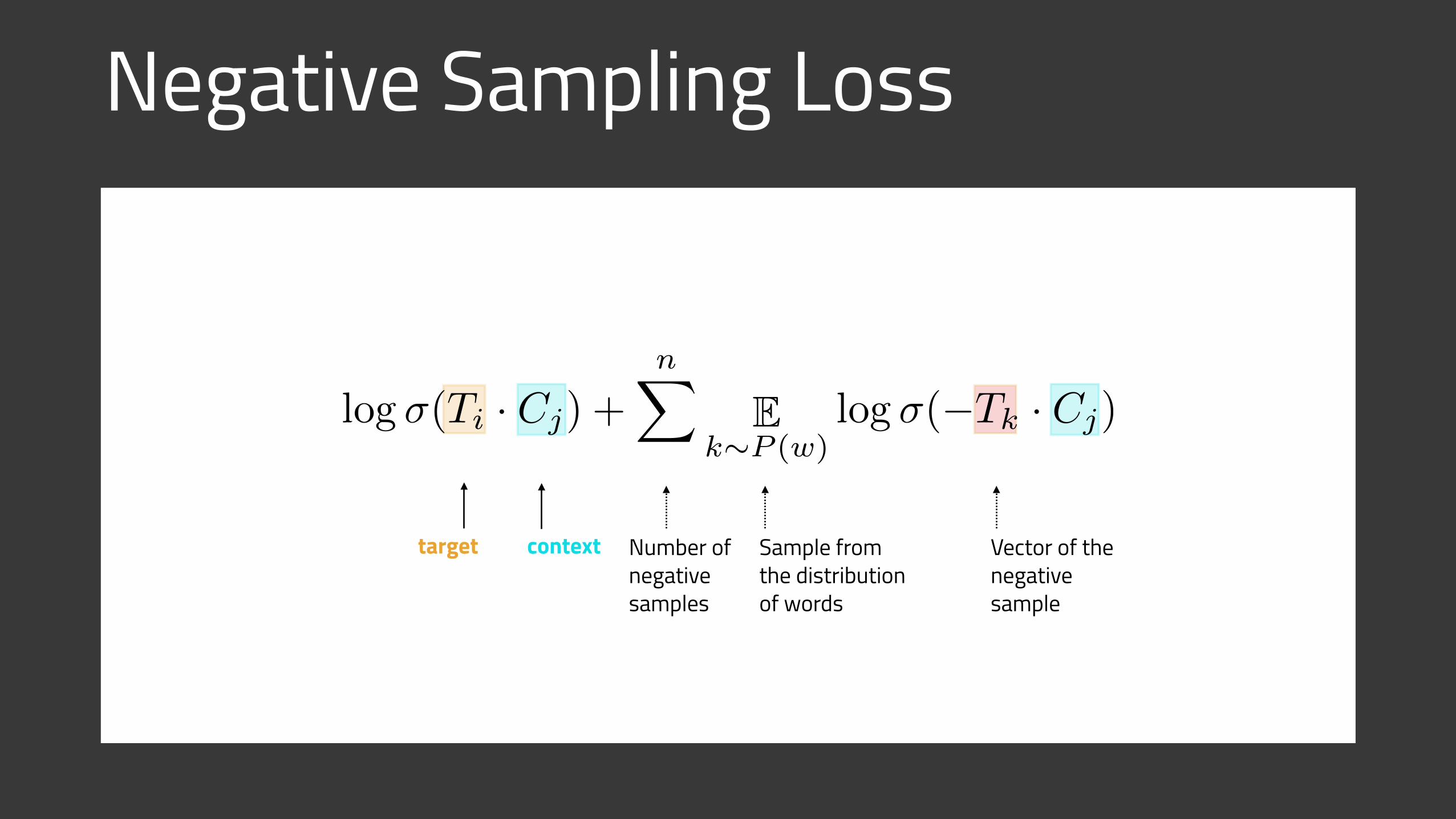
Negative Sampling Loss

Number of negative samples

target context Sample from the distribution of words

Vector of the negative sample

log �(Ti · Cj) +nX

Ek⇠P (w)

log �(�Tk · Cj)

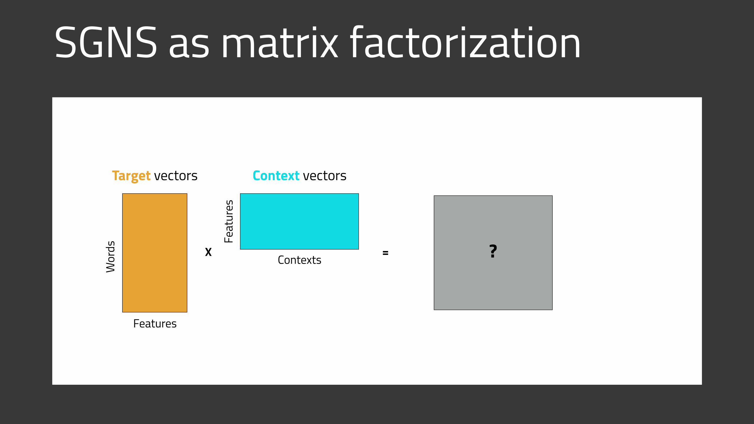
SGNS as matrix factorization

= ?

Wor

ds

Contexts

Features

Feat

ures

X


SGNS as matrix factorization

Wor

ds

Contexts

�log(k)= PMIX

Wor

ds

Contexts

Features

Feat

ures


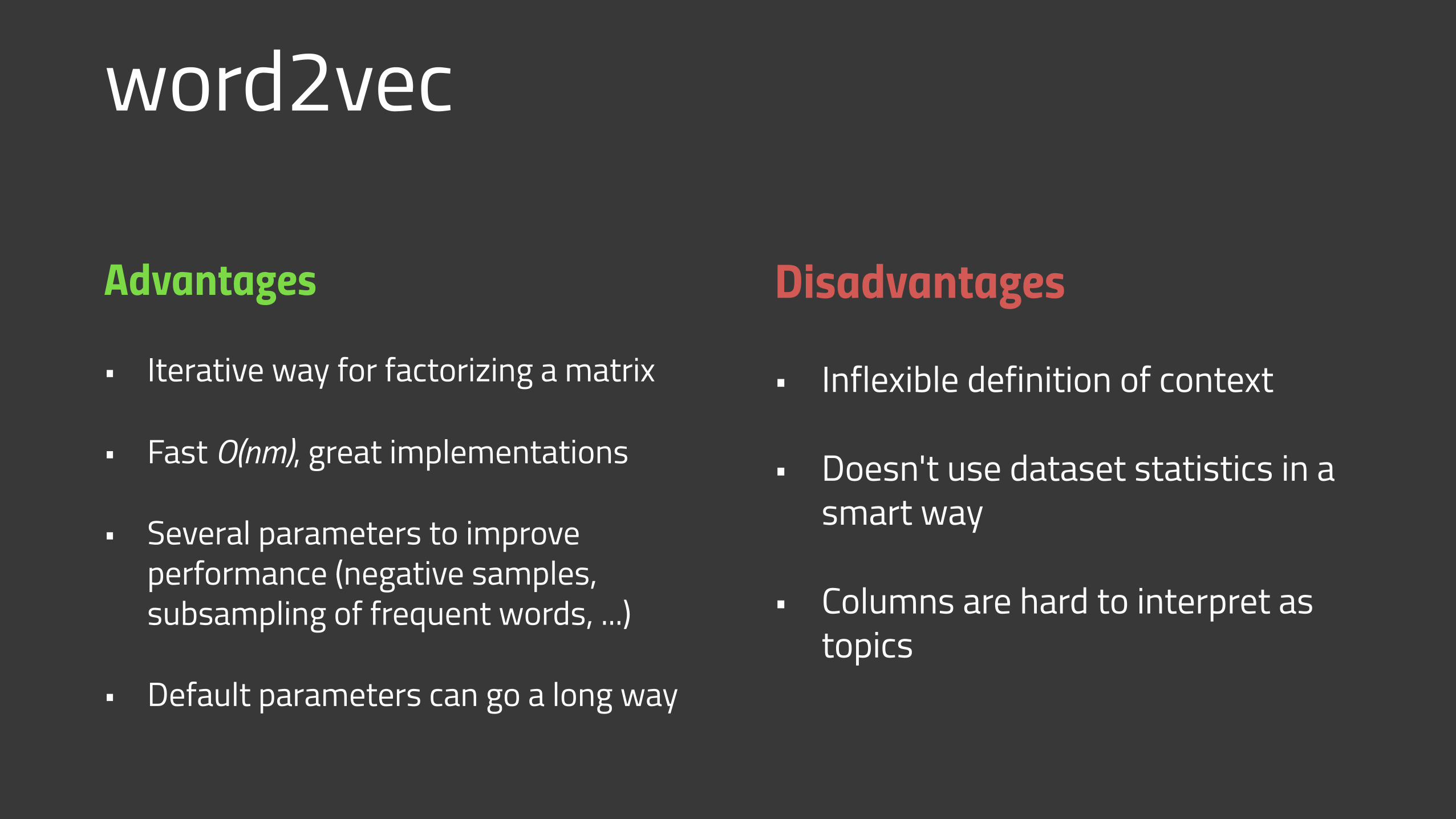
word2vec

Advantages

• Iterative way for factorizing a matrix

• Fast O(nm), great implementations

• Several parameters to improve performance (negative samples, subsampling of frequent words, ...)

• Default parameters can go a long way

Disadvantages

• Inflexible definition of context

• Doesn't use dataset statistics in a smart way

• Columns are hard to interpret as topics

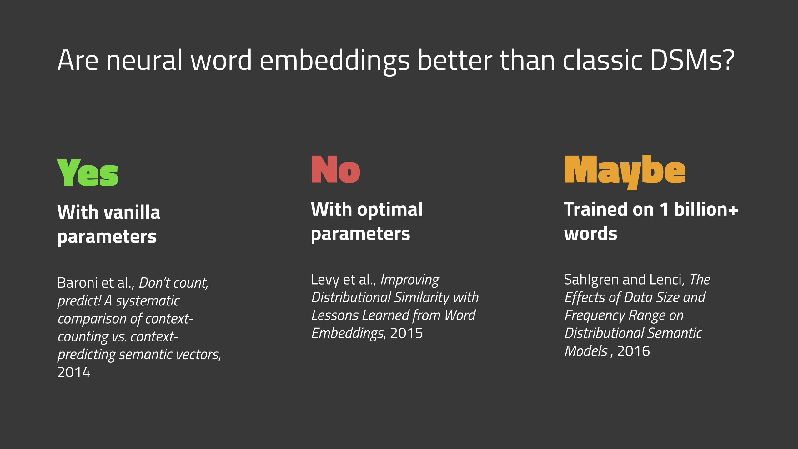
Are neural word embeddings better than classic DSMs?

Yes With vanilla parameters

Baroni et al., Don’t count, predict! A systematic comparison of context- counting vs. context-predicting semantic vectors, 2014

No With optimal parameters

Levy et al., Improving Distributional Similarity with Lessons Learned from Word Embeddings, 2015

Maybe Trained on 1 billion+ words

Sahlgren and Lenci, The Effects of Data Size and Frequency Range on Distributional Semantic Models , 2016

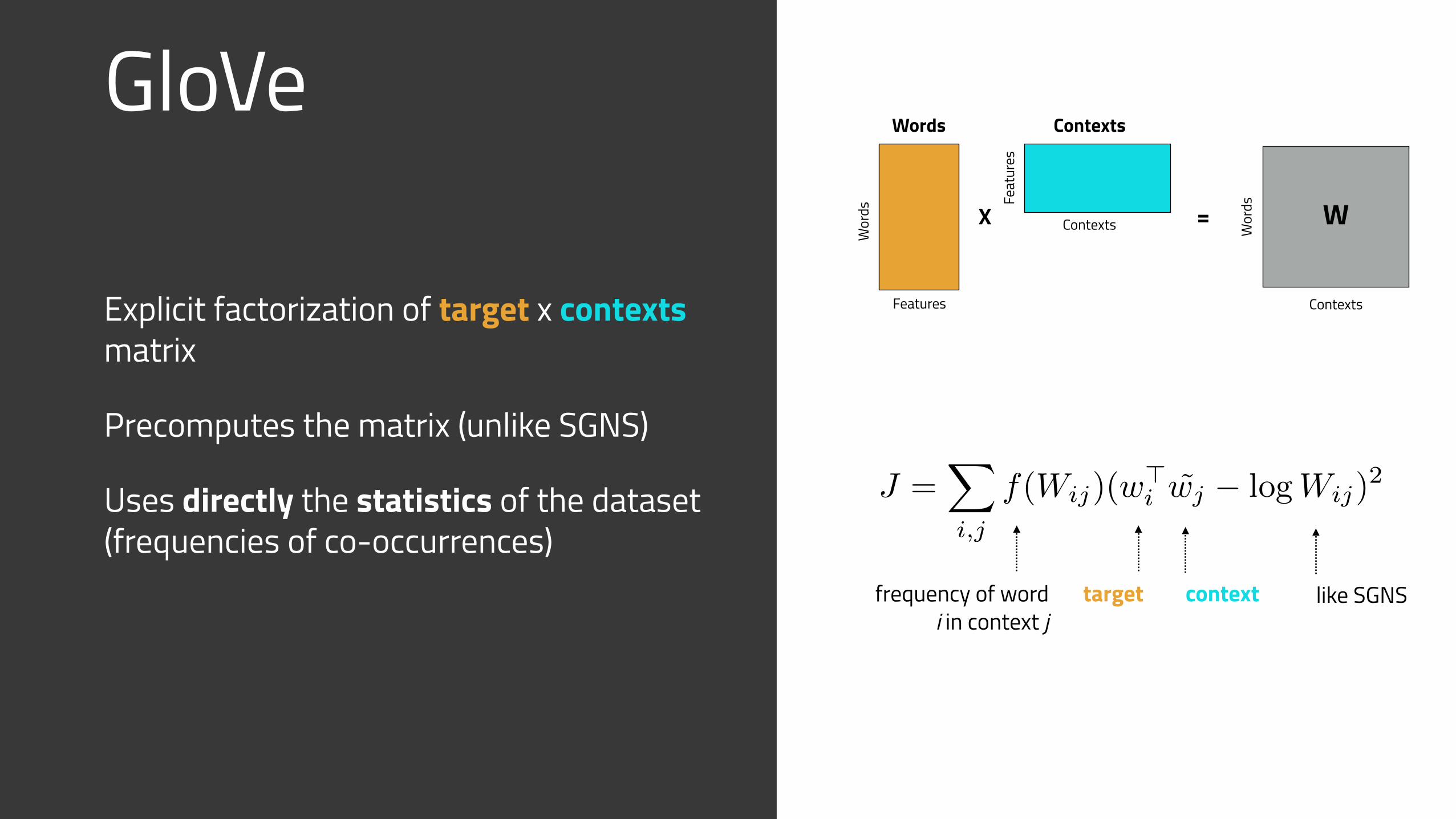
GloVe

Explicit factorization of target x contexts matrix

Precomputes the matrix (unlike SGNS)

Uses directly the statistics of the dataset (frequencies of co-occurrences)

J =X

i,j

f(Wij)(w>i wj � logWij)

2

frequency of word i in context j

target context like SGNS

Wor

ds

Contexts

= WX

Words Contexts

Wor

ds

Contexts

Features

Feat

ures

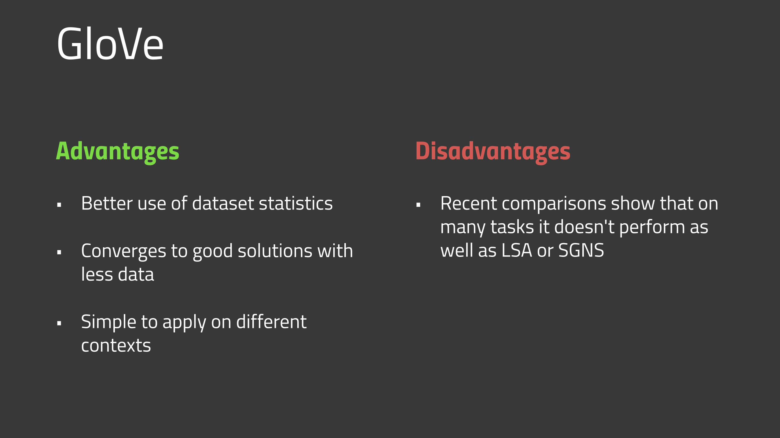
GloVe

Advantages

• Better use of dataset statistics

• Converges to good solutions with less data

• Simple to apply on different contexts

Disadvantages

• Recent comparisons show that on many tasks it doesn't perform as well as LSA or SGNS

Gaussian Embeddings and Multimodal Word Distributions

density

fw(~x) =KX

i=1

pw,i N [~x; ~µw,i,⌃w,i] (1)

=KX

i=1

pw,ip2⇡|⌃w,i|

e�12 (~x�~µw,i)>⌃�1

w,i(~x�~µw,i) ,

wherePK

i=1 pw,i = 1.

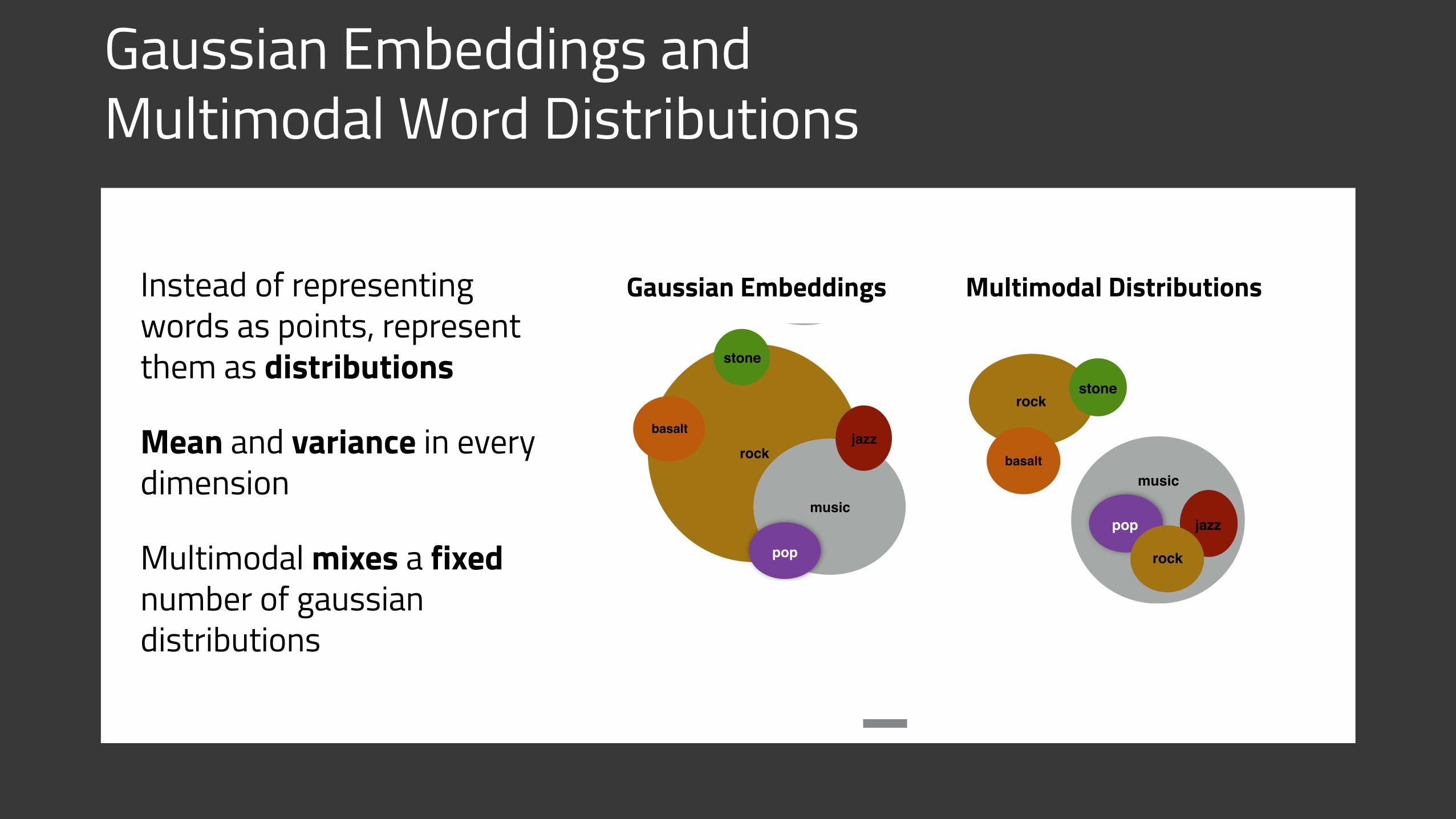
The mean vectors ~µw,i represent the location ofthe ith component of word w, and are akin to thepoint embeddings provided by popular approacheslike word2vec. pw,i represents the componentprobability (mixture weight), and ⌃w,i is the com-ponent covariance matrix, containing uncertaintyinformation. Our goal is to learn all of the modelparameters ~µw,i, pw,i,⌃w,i from a corpus of nat-ural sentences to extract semantic information ofwords. Each Gaussian component’s mean vectorof word w can represent one of the word’s distinctmeanings. For instance, one component of a pol-ysemous word such as ‘rock’ should represent themeaning related to ‘stone’ or ‘pebbles’, whereasanother component should represent the meaningrelated to music such as ‘jazz’ or ‘pop’. Figure1 illustrates our word embedding model, and thedifference between multimodal and unimodal rep-resentations, for words with multiple meanings.

3.2 Skip-Gram

The training objective for learning ✓ ={~µw,i, pw,i,⌃w,i} draws inspiration from thecontinuous skip-gram model (Mikolov et al.,2013a), where word embeddings are trained tomaximize the probability of observing a wordgiven another nearby word. This procedurefollows the distributional hypothesis that wordsoccurring in natural contexts tend to be semanti-cally related. For instance, the words ‘jazz’ and‘music’ tend to occur near one another more oftenthan ‘jazz’ and ‘cat’; hence, ‘jazz’ and ‘music’are more likely to be related. The learned wordrepresentation contains useful semantic informa-tion and can be used to perform a variety of NLPtasks such as word similarity analysis, sentimentclassification, modelling word analogies, or as apreprocessed input for complex system such asstatistical machine translation.

music

jazz

rock

basalt

pop

stone

rock

stone

Figure 1: Top: A Gaussian Mixture embed-ding, where each component corresponds to a dis-tinct meaning. Each Gaussian component is rep-resented by an ellipsoid, whose center is specifiedby the mean vector and contour surface specifiedby the covariance matrix, reflecting subtleties inmeaning and uncertainty. On the left, we show ex-amples of Gaussian mixture distributions of wordswhere Gaussian components are randomly initial-ized. After training, we see on the right thatone component of the word ‘rock’ is closer to‘stone’ and ‘basalt’, whereas the other componentis closer to ‘jazz’ and ‘pop’. We also demonstratethe entailment concept where the distribution ofthe more general word ‘music’ encapsulates wordssuch as ‘jazz’, ‘rock’, ‘pop’. Bottom: A Gaussianembedding model (Vilnis and McCallum, 2014).For words with multiple meanings, such as ‘rock’,the variance of the learned representation becomesunnecessarily large in order to assign some proba-bility to both meanings. Moreover, the mean vec-tor for such words can be pulled between two clus-ters, centering the mass of the distribution on a re-gion which is far from certain meanings.

3.3 Energy-based Max-Margin Objective

Each sample in the objective consists of two pairsof words, (w, c) and (w, c0). w is sampled from asentence in a corpus and c is a nearby word withina context window of length `. For instance, a wordw = ‘jazz’ which occurs in the sentence ‘I listento jazz music’ has context words (‘I’, ‘listen’, ‘to’, ‘music’). c0 is a negative context word (e.g. ‘air-plane’) obtained from random sampling.

The objective is to maximize the energy be-tween words that occur near each other, w and c,and minimize the energy between w and its nega-tive context c0. This approach is similar to neg-

Instead of representing words as points, represent them as distributions

Mean and variance in every dimension

Multimodal mixes a fixed number of gaussian distributions

density

fw(~x) =KX

i=1

pw,i N [~x; ~µw,i,⌃w,i] (1)

=KX

i=1

pw,ip2⇡|⌃w,i|

e�12 (~x�~µw,i)>⌃�1

w,i(~x�~µw,i) ,

wherePK

i=1 pw,i = 1.

The mean vectors ~µw,i represent the location ofthe ith component of word w, and are akin to thepoint embeddings provided by popular approacheslike word2vec. pw,i represents the componentprobability (mixture weight), and ⌃w,i is the com-ponent covariance matrix, containing uncertaintyinformation. Our goal is to learn all of the modelparameters ~µw,i, pw,i,⌃w,i from a corpus of nat-ural sentences to extract semantic information ofwords. Each Gaussian component’s mean vectorof word w can represent one of the word’s distinctmeanings. For instance, one component of a pol-ysemous word such as ‘rock’ should represent themeaning related to ‘stone’ or ‘pebbles’, whereasanother component should represent the meaningrelated to music such as ‘jazz’ or ‘pop’. Figure1 illustrates our word embedding model, and thedifference between multimodal and unimodal rep-resentations, for words with multiple meanings.

3.2 Skip-Gram

The training objective for learning ✓ ={~µw,i, pw,i,⌃w,i} draws inspiration from thecontinuous skip-gram model (Mikolov et al.,2013a), where word embeddings are trained tomaximize the probability of observing a wordgiven another nearby word. This procedurefollows the distributional hypothesis that wordsoccurring in natural contexts tend to be semanti-cally related. For instance, the words ‘jazz’ and‘music’ tend to occur near one another more oftenthan ‘jazz’ and ‘cat’; hence, ‘jazz’ and ‘music’are more likely to be related. The learned wordrepresentation contains useful semantic informa-tion and can be used to perform a variety of NLPtasks such as word similarity analysis, sentimentclassification, modelling word analogies, or as apreprocessed input for complex system such asstatistical machine translation.

music

rock

basalt

stone

music

jazz

pop

Figure 1: Top: A Gaussian Mixture embed-ding, where each component corresponds to a dis-tinct meaning. Each Gaussian component is rep-resented by an ellipsoid, whose center is specifiedby the mean vector and contour surface specifiedby the covariance matrix, reflecting subtleties inmeaning and uncertainty. On the left, we show ex-amples of Gaussian mixture distributions of wordswhere Gaussian components are randomly initial-ized. After training, we see on the right thatone component of the word ‘rock’ is closer to‘stone’ and ‘basalt’, whereas the other componentis closer to ‘jazz’ and ‘pop’. We also demonstratethe entailment concept where the distribution ofthe more general word ‘music’ encapsulates wordssuch as ‘jazz’, ‘rock’, ‘pop’. Bottom: A Gaussianembedding model (Vilnis and McCallum, 2014).For words with multiple meanings, such as ‘rock’,the variance of the learned representation becomesunnecessarily large in order to assign some proba-bility to both meanings. Moreover, the mean vec-tor for such words can be pulled between two clus-ters, centering the mass of the distribution on a re-gion which is far from certain meanings.

3.3 Energy-based Max-Margin Objective

Each sample in the objective consists of two pairsof words, (w, c) and (w, c0). w is sampled from asentence in a corpus and c is a nearby word withina context window of length `. For instance, a wordw = ‘jazz’ which occurs in the sentence ‘I listento jazz music’ has context words (‘I’, ‘listen’, ‘to’, ‘music’). c0 is a negative context word (e.g. ‘air-plane’) obtained from random sampling.

The objective is to maximize the energy be-tween words that occur near each other, w and c,and minimize the energy between w and its nega-tive context c0. This approach is similar to neg-

Gaussian Embeddings Multimodal Distributions

Gaussian Embeddings and Multimodal Word Distributions

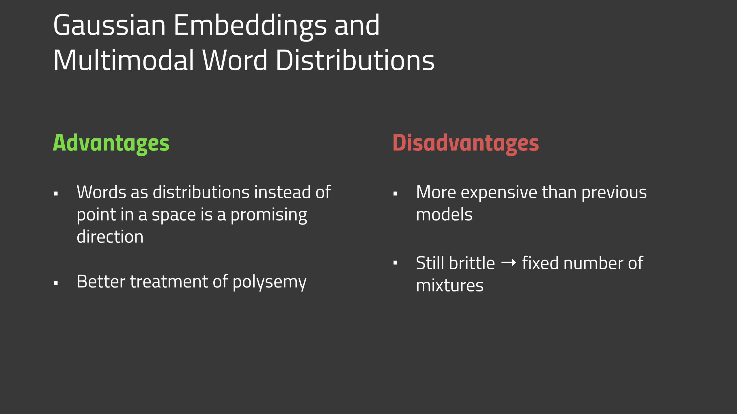
Advantages

• Words as distributions instead of point in a space is a promising direction

• Better treatment of polysemy

Disadvantages

• More expensive than previous models

• Still brittle → fixed number of mixtures

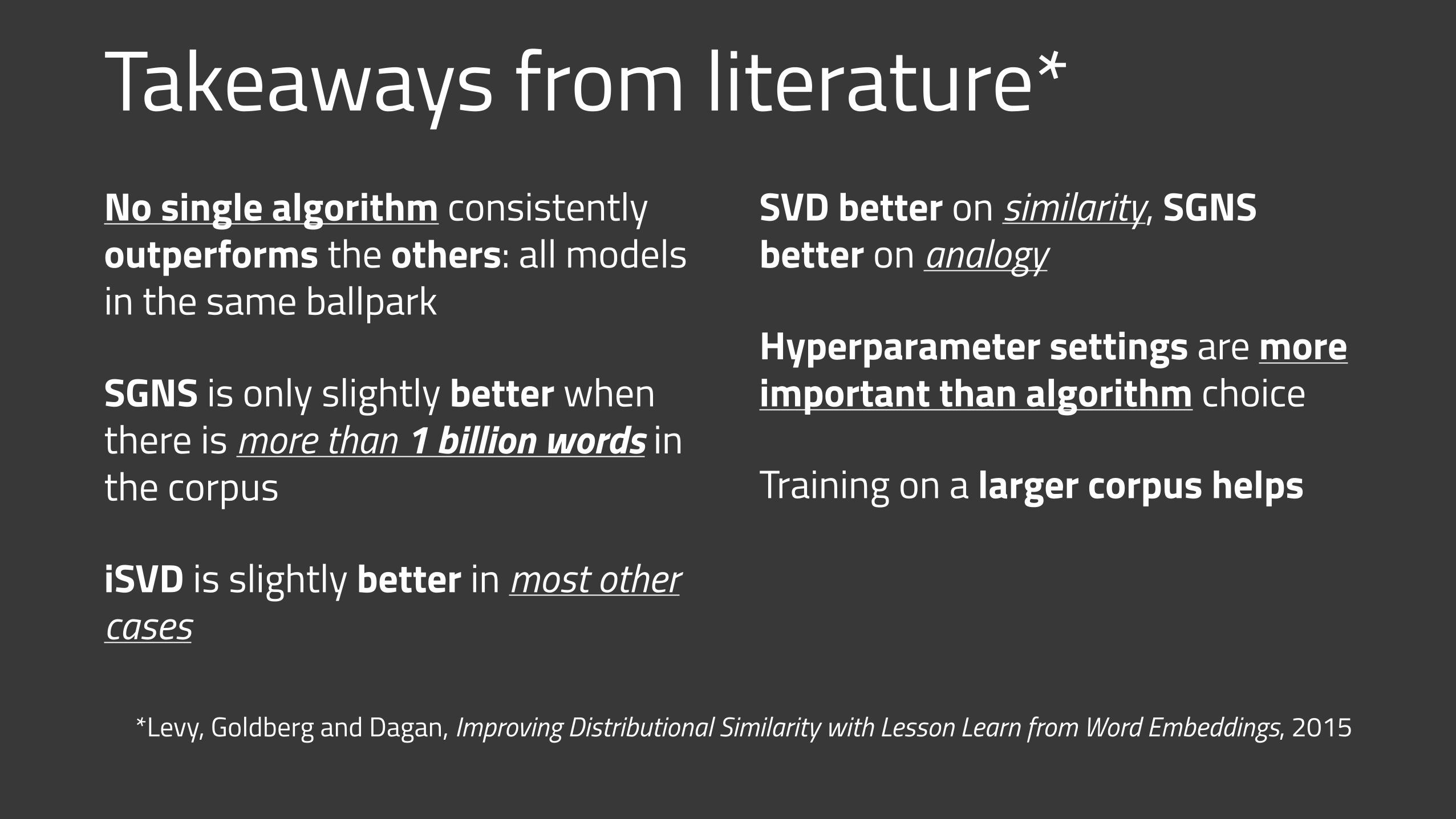
Takeaways from literature*No single algorithm consistently outperforms the others: all models in the same ballpark

SGNS is only slightly better when there is more than 1 billion words in the corpus

iSVD is slightly better in most other cases

SVD better on similarity, SGNS better on analogy

Hyperparameter settings are more important than algorithm choice

Training on a larger corpus helps

*Levy, Goldberg and Dagan, Improving Distributional Similarity with Lesson Learn from Word Embeddings, 2015

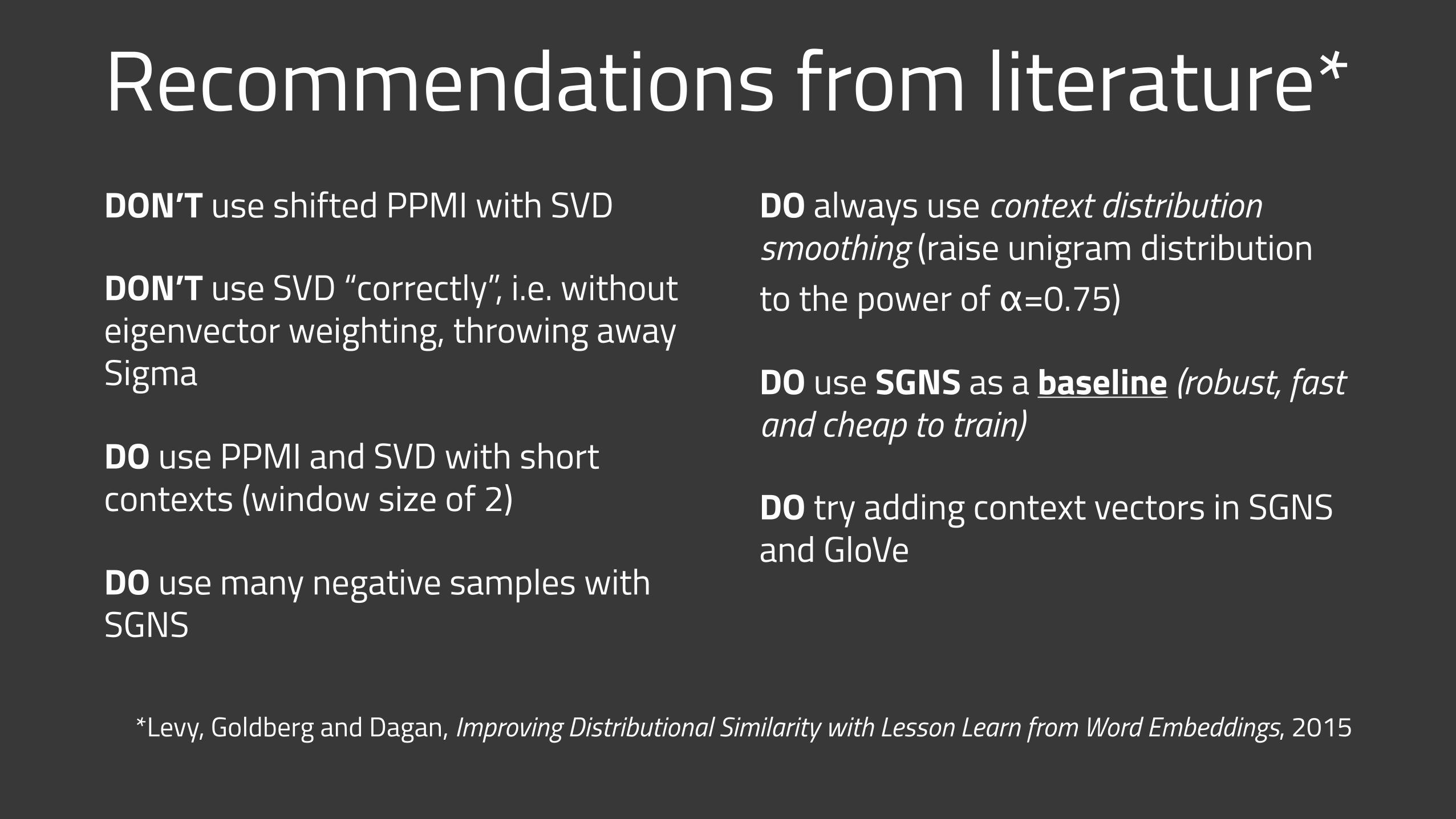
Recommendations from literature*DON’T use shifted PPMI with SVD

DON’T use SVD “correctly”, i.e. without eigenvector weighting, throwing away Sigma

DO use PPMI and SVD with short contexts (window size of 2)

DO use many negative samples with SGNS

DO always use context distribution smoothing (raise unigram distribution to the power of α=0.75)

DO use SGNS as a baseline (robust, fast and cheap to train)

DO try adding context vectors in SGNS and GloVe

*Levy, Goldberg and Dagan, Improving Distributional Similarity with Lesson Learn from Word Embeddings, 2015

Open questions and current trends

Compositionality

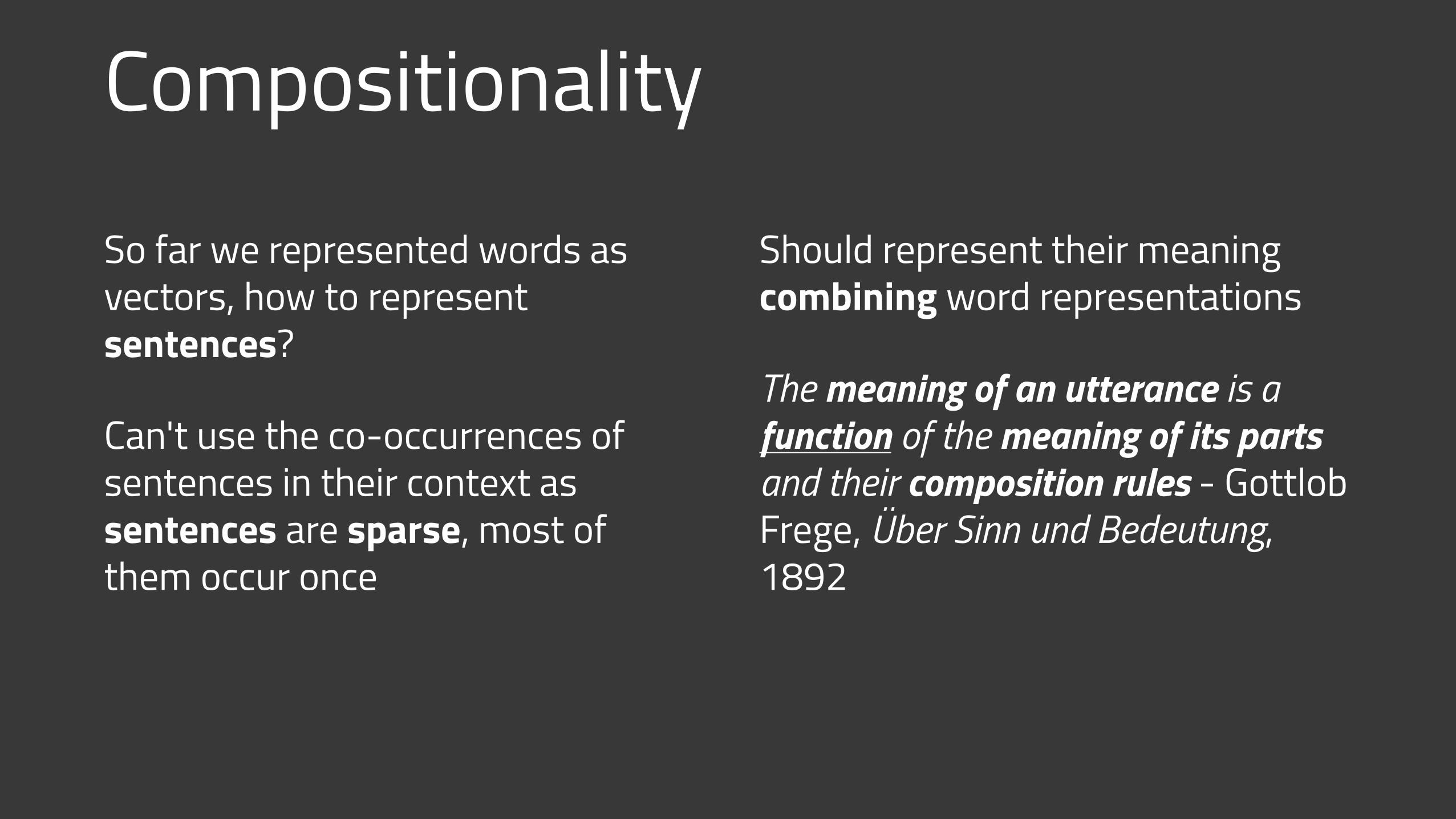
So far we represented words as vectors, how to represent sentences?

Can't use the co-occurrences of sentences in their context as sentences are sparse, most of them occur once

Should represent their meaning combining word representations

The meaning of an utterance is a function of the meaning of its parts and their composition rules - Gottlob Frege, Über Sinn und Bedeutung, 1892

Composition operators

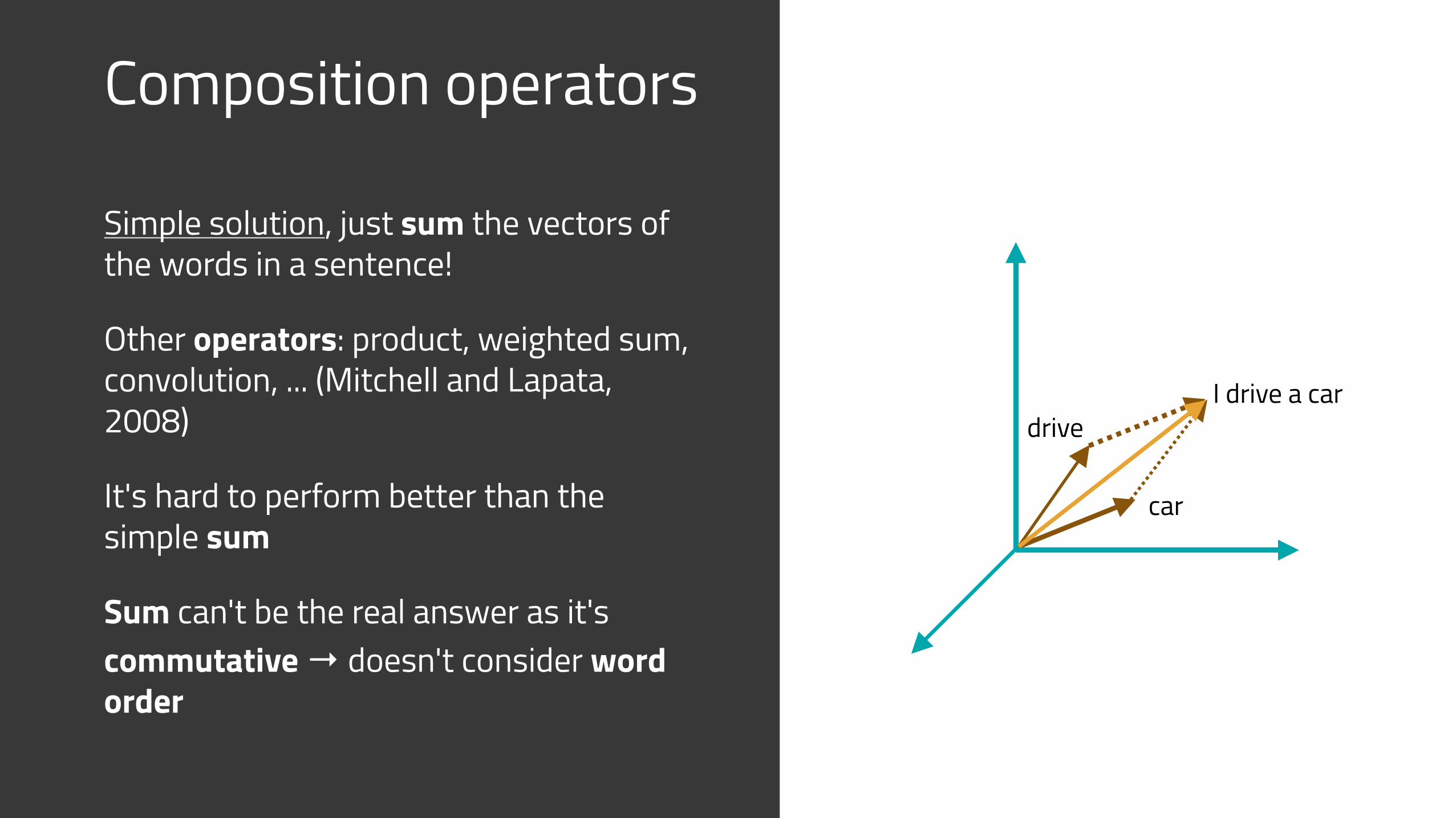
Simple solution, just sum the vectors of the words in a sentence!

Other operators: product, weighted sum, convolution, ... (Mitchell and Lapata, 2008)

It's hard to perform better than the simple sum

Sum can't be the real answer as it's commutative → doesn't consider word order

drive

car

I drive a car

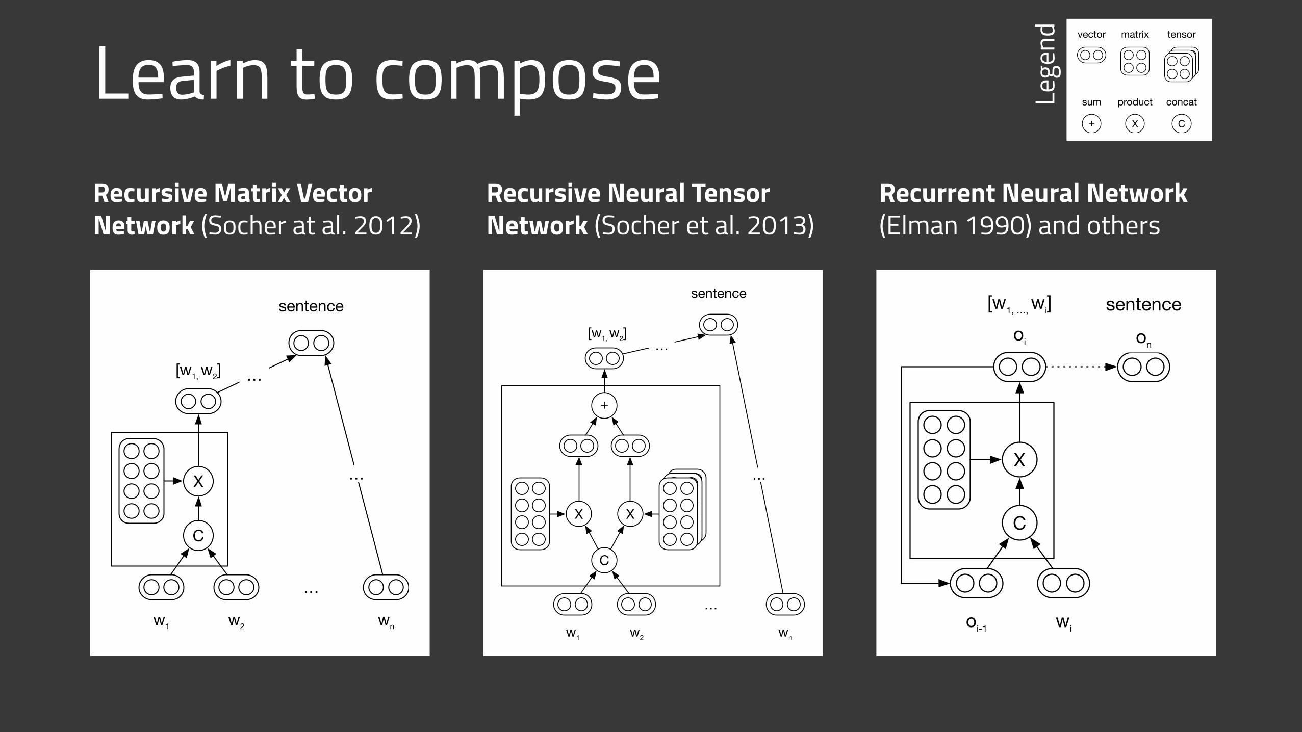
Learn to composeRecursive Matrix Vector Network (Socher at al. 2012)

Recursive Neural Tensor Network (Socher et al. 2013)

Recurrent Neural Network (Elman 1990) and others

C

X

oi-1 wi

sentence[w1, …, wi]oi on

C

X

…

…

…

w1 w2 wn

sentence

[w1, w2]

C

X

…

…

…

w1 w2 wn

sentence

[w1, w2]

X

+

vector matrix tensor

CX+

sum product concatLege

nd

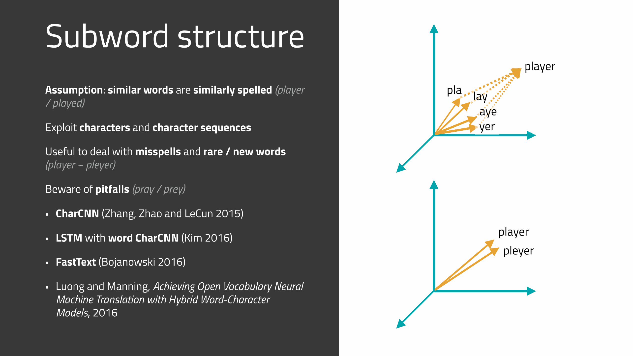
Subword structureAssumption: similar words are similarly spelled (player / played)

Exploit characters and character sequences

Useful to deal with misspells and rare / new words (player ~ pleyer)

Beware of pitfalls (pray / prey)

• CharCNN (Zhang, Zhao and LeCun 2015)

• LSTM with word CharCNN (Kim 2016)

• FastText (Bojanowski 2016)

• Luong and Manning, Achieving Open Vocabulary Neural Machine Translation with Hybrid Word-Character Models, 2016

pla

player

playerpleyer

layayeyer

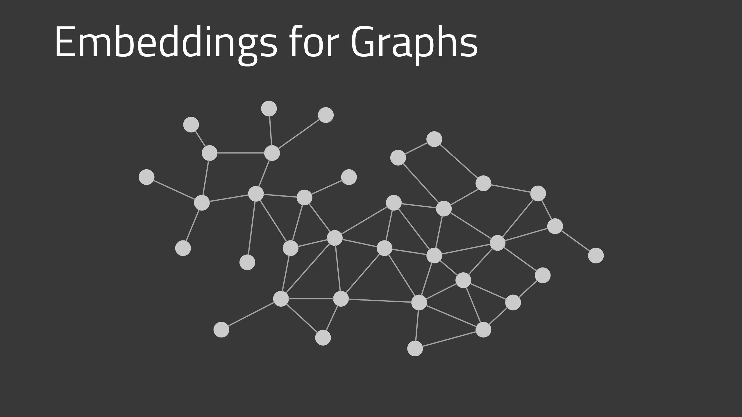
Embeddings for Graphs

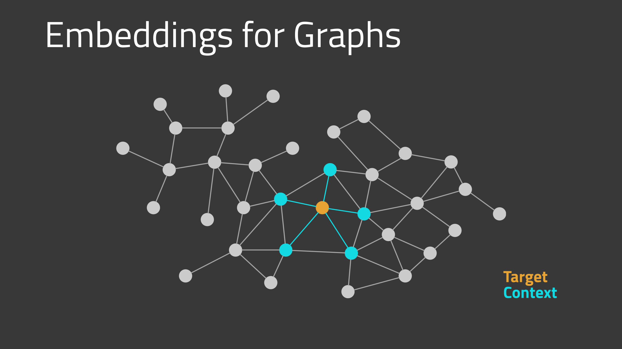
Embeddings for Graphs

TargetContext

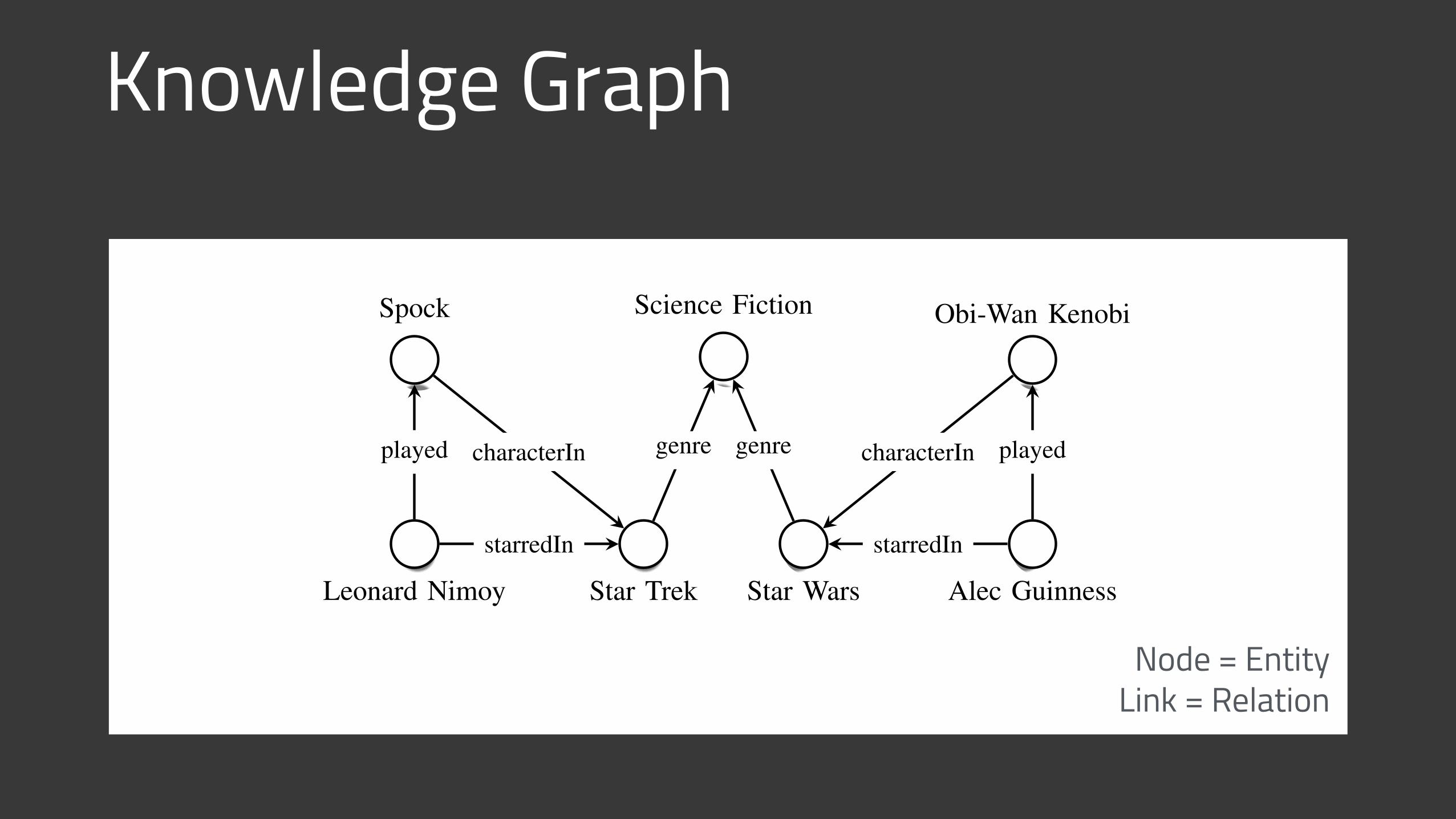
Knowledge Graph2

Leonard Nimoy

Spock

Star Trek

Science Fiction

Star Wars Alec Guinness

Obi-Wan Kenobi

starredIn

played characterIn genre

starredIn

playedcharacterIngenre

Fig. 1. Sample knowledge graph. Nodes represent entities, edge labels representtypes of relations, edges represent existing relationships.

frames [13]. More recently, it has been used in the SemanticWeb community with the purpose of creating a “web of data”that is readable by machines [14]. While this vision of theSemantic Web remains to be fully realized, parts of it havebeen achieved. In particular, the concept of linked data [15, 16]has gained traction, as it facilitates publishing and interlinkingdata on the Web in relational form using the W3C ResourceDescription Framework (RDF) [17, 18]. (For an introductionto knowledge representation, see e.g. [11, 19, 20]).

In this article, we will loosely follow the RDF standard andrepresent facts in the form of binary relationships, in particular(subject, predicate, object) (SPO) triples, where subject andobject are entities and predicate is the relation betweenthem. (We discuss how to represent higher-arity relationsin Section X-A.) The existence of a particular SPO tripleindicates an existing fact, i.e., that the respective entities are ina relationship of the given type. For instance, the information

Leonard Nimoy was an actor who played the char-acter Spock in the science-fiction movie Star Trek

can be expressed via the following set of SPO triples:

subject predicate object

(LeonardNimoy, profession, Actor)(LeonardNimoy, starredIn, StarTrek)(LeonardNimoy, played, Spock)(Spock, characterIn, StarTrek)(StarTrek, genre, ScienceFiction)

We can combine all the SPO triples together to form a multi-graph, where nodes represent entities (all subjects and objects),and directed edges represent relationships. The direction of anedge indicates whether entities occur as subjects or objects, i.e.,an edge points from the subject to the object. Different relationsare represented via different types of edges (also called edgelabels). This construction is called a knowledge graph (KG),or sometimes a heterogeneous information network [21].) SeeFigure 1 for an example.

In addition to being a collection of facts, knowledge graphsoften provide type hierarchies (Leonard Nimoy is an actor,which is a person, which is a living thing) and type constraints(e.g., a person can only marry another person, not a thing).

B. Open vs. closed world assumptionWhile existing triples always encode known true relationships

(facts), there are different paradigms for the interpretation of

TABLE IKNOWLEDGE BASE CONSTRUCTION PROJECTS

Method Schema Examples

Curated Yes Cyc/OpenCyc [23], WordNet [24],UMLS [25]

Collaborative Yes Wikidata [26], Freebase [7]

Auto. Semi-Structured Yes YAGO [4, 27], DBPedia [5],Freebase [7]

Auto. Unstructured Yes Knowledge Vault [28], NELL [6],PATTY [29], PROSPERA [30],DeepDive/Elementary [31]

Auto. Unstructured No ReVerb [32], OLLIE [33],PRISMATIC [34]

non-existing triples:‚ Under the closed world assumption (CWA), non-existing

triples indicate false relationships. For example, the factthat in Figure 1 there is no starredIn edge from LeonardNimoy to Star Wars is interpreted to mean that Nimoydefinitely did not star in this movie.

‚ Under the open world assumption (OWA), a non-existingtriple is interpreted as unknown, i.e., the correspondingrelationship can be either true or false. Continuing with theabove example, the missing edge is not interpreted to meanthat Nimoy did not star in Star Wars. This more cautiousapproach is justified, since KGs are known to be veryincomplete. For example, sometimes just the main actorsin a movie are listed, not the complete cast. As anotherexample, note that even the place of birth attribute, whichyou might think would be typically known, is missing for71% of all people included in Freebase [22].

RDF and the Semantic Web make the open-world assumption.In Section VII-B we also discuss the local closed worldassumption (LCWA), which is often used for training relationalmodels.

C. Knowledge base constructionCompleteness, accuracy, and data quality are important

parameters that determine the usefulness of knowledge basesand are influenced by the way knowledge bases are constructed.We can classify KB construction methods into four maingroups:

‚ In curated approaches, triples are created manually by aclosed group of experts.

‚ In collaborative approaches, triples are created manuallyby an open group of volunteers.

‚ In automated semi-structured approaches, triples areextracted automatically from semi-structured text (e.g.,infoboxes in Wikipedia) via hand-crafted rules, learnedrules, or regular expressions.

‚ In automated unstructured approaches, triples are ex-tracted automatically from unstructured text via machinelearning and natural language processing techniques (see,e.g., [9] for a review).

Construction of curated knowledge bases typically leads tohighly accurate results, but this technique does not scale well

Node = Entity Link = Relation

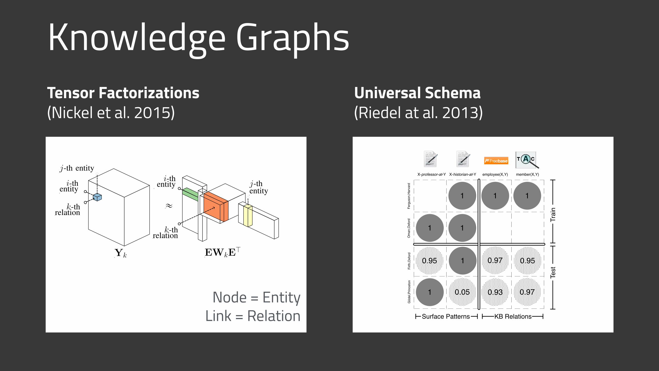
Knowledge GraphsTensor Factorizations (Nickel et al. 2015)

Universal Schema (Riedel at al. 2013)

7

«

i-thentity

j-th entity

k-threlation

i-thentity j-th

entity

k-threlation

Yk EWkEJ

Fig. 4. RESCAL as a tensor factorization of the adjacency tensor Y.

while it occurs in the triple xpiq as the object of a relationshipof type q. However, the predictions fijk “ eJ

iWkej and

fpiq “ eJpWqei both use the same latent representation ei

of the i-th entity. Since all parameters are learned jointly,these shared representations permit to propagate informationbetween triples via the latent representations of entities and theweights of relations. This allows the model to capture globaldependencies in the data.

Semantic embeddings: The shared entity representationsin RESCAL capture also the similarity of entities in therelational domain, i.e., that entities are similar if they areconnected to similar entities via similar relations [65]. Forinstance, if the representations of ei and ep are similar, thepredictions fijk and fpjk will have similar values. In return,entities with many similar observed relationships will havesimilar latent representations. This property can be exploited forentity resolution and has also enabled large-scale hierarchicalclustering on relational data [63, 64]. Moreover, since relationalsimilarity is expressed via the similarity of vectors, the latentrepresentations ei can act as proxies to give non-relationalmachine learning algorithms such as k-means or kernel methodsaccess to the relational similarity of entities.

Connection to tensor factorization: RESCAL is similarto methods used in recommendation systems [66], and totraditional tensor factorization methods [67]. In matrix notation,Equation (3) can be written compactly as as Fk “ EWkEJ,where Fk P RNeˆNe is the matrix holding all scores for thek-th relation and the i-th row of E P RNeˆHe holds the latentrepresentation of ei. See Figure 4 for an illustration. In thefollowing, we will use this tensor representation to derive avery efficient algorithm for parameter estimation.

Fitting the model: If we want to compute a probabilisticmodel, the parameters of RESCAL can be estimated byminimizing the log-loss using gradient-based methods such asstochastic gradient descent [68]. RESCAL can also be com-puted as a score-based model, which has the main advantagethat we can estimate the parameters ⇥ very efficiently: Dueto its tensor structure and due to the sparsity of the data, ithas been shown that the RESCAL model can be computedvia a sequence of efficient closed-form updates when usingthe squared-loss [63, 64]. In this setting, it has been shownanalytically that a single update of E and Wk scales linearlywith the number of entities Ne, linearly with the number ofrelations Nr, and linearly with the number of observed triples,i.e., the number of non-zero entries in Y [64]. We call this

algorithm RESCAL-ALS.9 In practice, a small number (say 30to 50) of iterated updates are often sufficient for RESCAL-ALSto arrive at stable estimates of the parameters. Given a currentestimate of E, the updates for each Wk can be computed inparallel to improve the scalability on knowledge graphs witha large number of relations. Furthermore, by exploiting thespecial tensor structure of RESCAL, we can derive improvedupdates for RESCAL-ALS that compute the estimates for theparameters with a runtime complexity of OpH3

eq for a single

update (as opposed to a runtime complexity of OpH5e

q fornaive updates) [65, 69]. In summary, for relational domainsthat can be explained via a moderate number of latent features,RESCAL-ALS is highly scalable and very fast to compute.For more detail on RESCAL-ALS see also Equation (26) inSection VII.

Decoupled Prediction: In Equation (3), the probabilityof single relationship is computed via simple matrix-vectorproducts in OpH2

eq time. Hence, once the parameters have been

estimated, the computational complexity to predict the score ofa triple depends only on the number of latent features and isindependent of the size of the graph. However, during parameterestimation, the model can capture global dependencies due tothe shared latent representations.

Relational learning results: RESCAL has been shownto achieve state-of-the-art results on a number of relationallearning tasks. For instance, [63] showed that RESCALprovides comparable or better relationship prediction resultson a number of small benchmark datasets compared toMarkov Logic Networks (with structure learning) [70], theInfinite (Hidden) Relational model [71, 72], and BayesianClustered Tensor Factorization [73]. Moreover, RESCAL hasbeen used for link prediction on entire knowledge graphs suchas YAGO and DBpedia [64, 74]. Aside from link prediction,RESCAL has also successfully been applied to SRL tasks suchas entity resolution and link-based clustering. For instance,RESCAL has shown state-of-the-art results in predicting whichauthors, publications, or publication venues are likely to beidentical in publication databases [63, 65]. Furthermore, thesemantic embedding of entities computed by RESCAL hasbeen exploited to create taxonomies for uncategorized data viahierarchical clusterings of entities in the embedding space [75].

B. Other tensor factorization modelsVarious other tensor factorization methods have been ex-

plored for learning from knowledge graphs and multi-relationaldata. [76, 77] factorized adjacency tensors using the CPtensor decomposition to analyze the link structure of Webpages and Semantic Web data respectively. [78] appliedpairwise interaction tensor factorization [79] to predict triplesin knowledge graphs. [80] applied factorization machines tolarge uni-relational datasets in recommendation settings. [81]proposed a tensor factorization model for knowledge graphswith a very large number of different relations.

It is also possible to use discrete latent factors. [82] proposedBoolean tensor factorization to disambiguate facts extractedwith OpenIE methods and applied it to large datasets [83]. In

9ALS stands for Alternating Least-Squares

Trai

n

0.95

Test

Surface Patterns KB Relations

X-professor-at-Y

1

1

0.05

X-historian-at-Y employee(X,Y) member(X,Y)

1 1

1

1 0.97

Rel. Extraction

1 0.93 0.97

Cluster Align

Reasoning with Universal Schema

Ferg

uson

,Har

vard

Om

an,O

xfor

dFi

rth,O

xfor

dG

ödel

,Prin

ceto

n

0.95

Figure 1: Filling up a database of universal schema.Dark circles are observed facts, shaded circles are in-ferred facts. Relation Extraction (RE) maps surface pat-tern relations (and other features) to structured relations.Surface form clustering models correlations between pat-terns, and can be fed into RE (Yao et al., 2011). Databasealignment and integration models correlations betweenstructured relations (not done in this work). Reasoningwith the universal schema incorporates these tasks in ajoint fashion.

introduce a series of exponential family models thatestimate this probability using a natural parameter✓r,t and the logistic function:

p (yr,t = 1|✓r,t) := � (✓r,t) =1

1 + exp (�✓r,t).

We will first describe our models through differ-ent definitions of the natural parameter ✓r,t. In eachcase ✓r,t will be a function of r, t and a set of weightsand/or latent feature vectors. In section 2.5 we willthen show how these weights and vectors can be es-timated based on the observed facts O.

Notice that we can interpret p (yr,t = 1) as theprobability that a customer t likes product r. Thisanalogy allows us to draw from a large body of workin collaborative filtering, such as work in probabilis-tic matrix factorization and implicit feedback.

2.1 Latent Feature Model

One way to define ✓r,t is through a latent featuremodel F. Here we measure compatibility betweenrelation r and tuple t as dot product of two latentfeature representations of size KF: ar for relation r,and vt for tuple t. This gives:

✓Fr,t :=

KFX

k

ar,kvt,k.

This corresponds to generalized PCA (Collins et al.,2001), a model were the matrix ⇥ = (✓r,t) of naturalparameters is defined as the low rank factorizationAV.

Notice that we intentionally omit any per-relationbias-terms. In section 4 we evaluate ranked answersto queries on a per-relation basis, and a per-relationbias term will have no effect on ranking facts of thesame relation. Also consider that such latent featuremodels can capture asymmetry by assigning morepeaked vectors to specific relations, and more uni-form vectors to general relations.

2.2 Neighborhood Model

We can interpolate the confidence for a given tupleand relation based on the trueness of other similarrelations for the same tuple. In collaborative filter-ing this is referred to as a neighborhood-based ap-proach (Koren, 2008). In terms of our natural pa-rameter, we implement a neighborhood model N viaa set of weights wr,r0 , where each corresponds to adirected association strength between relations r andr0. For a given tuple t and relation r we then sumup the weights corresponding to all relations r0 thathave been observed for tuple t:

✓Nr,t :=

X

(r0,t)2O\{(r,t)}

wr,r0 .

Notice that the neighborhood model amounts toa collection of local log-linear classifiers, one foreach relation r with feature functions fr,r0 (t) =I [r0 6= r ^ (r0, t) 2 O] and weights wr. This meansthat in contrast to model F, this model cannot har-ness any synergies between textual and pre-existingDB relations.

Node = Entity Link = Relation

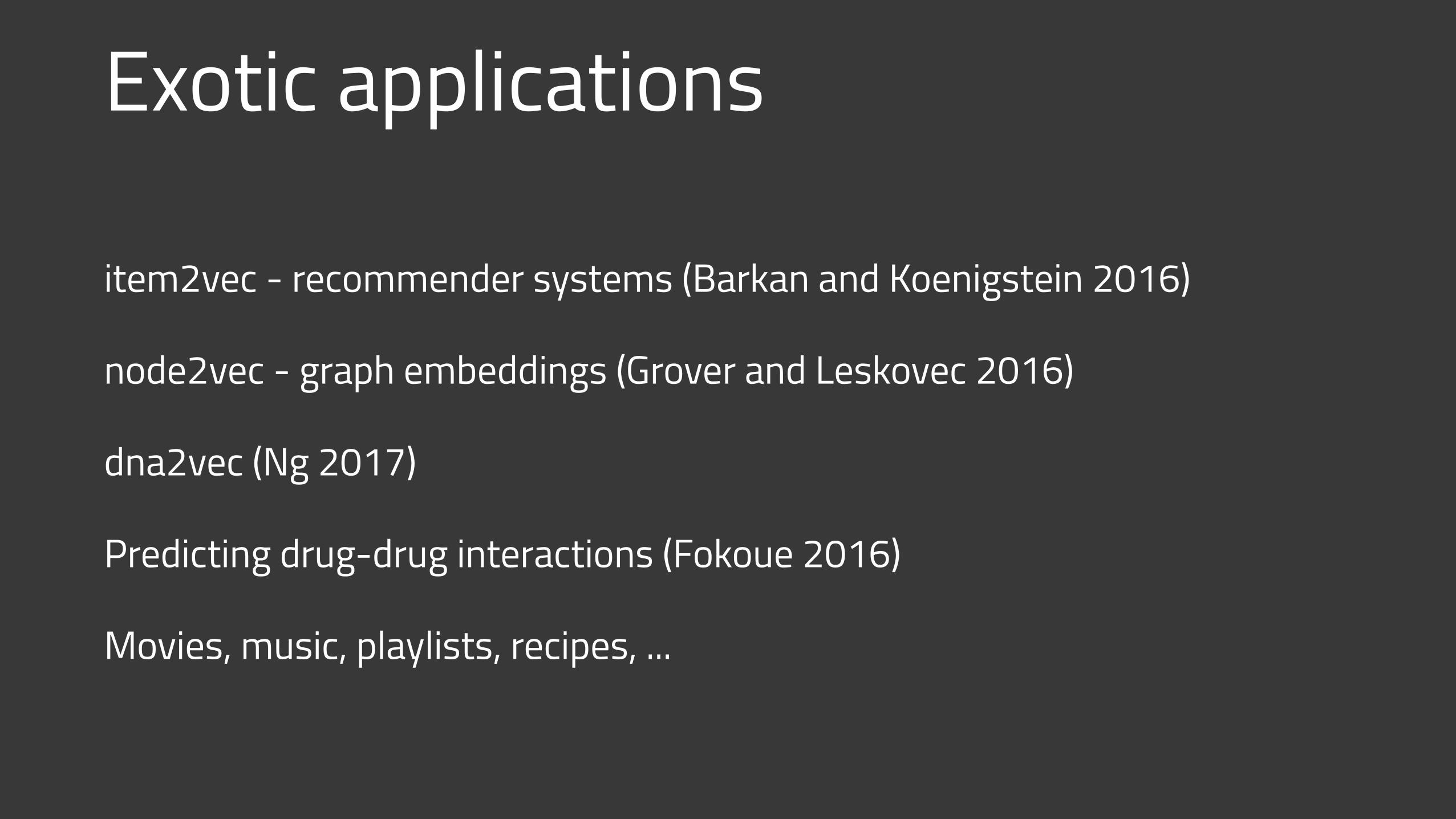
Exotic applications

item2vec - recommender systems (Barkan and Koenigstein 2016)

node2vec - graph embeddings (Grover and Leskovec 2016)

dna2vec (Ng 2017)

Predicting drug-drug interactions (Fokoue 2016)

Movies, music, playlists, recipes, ...

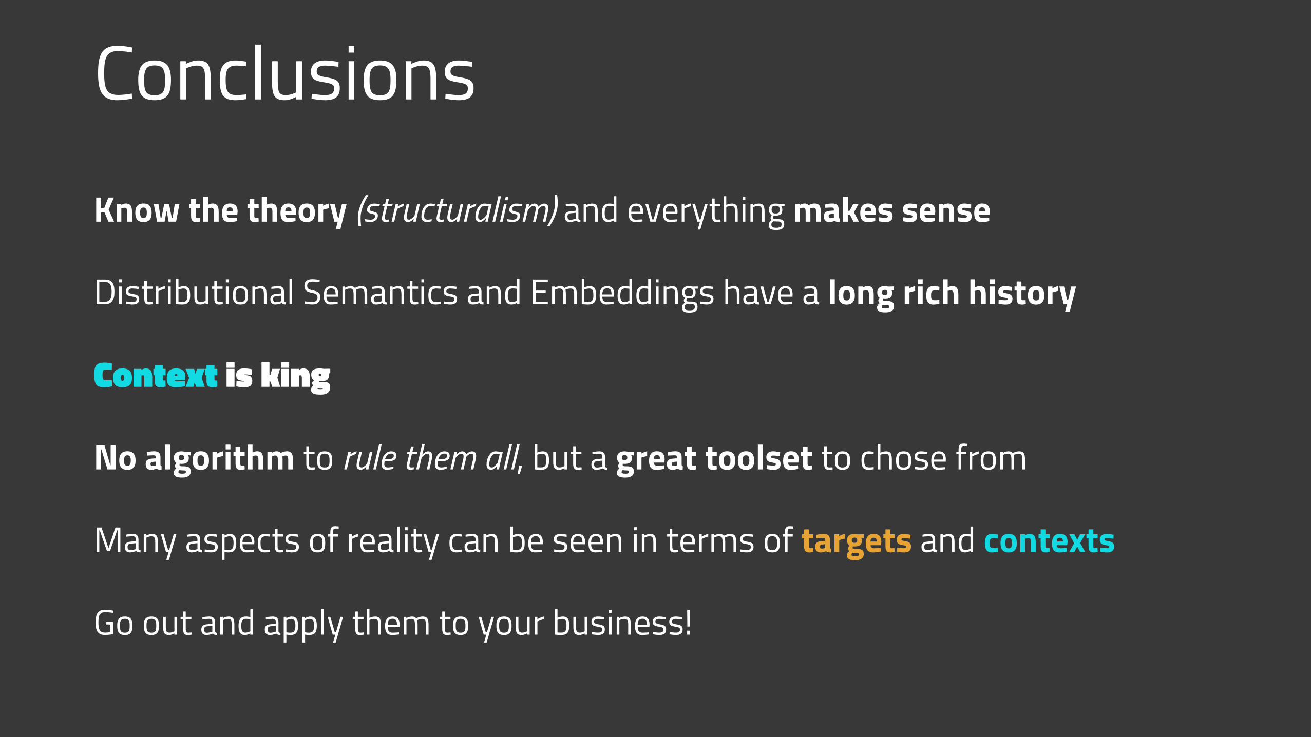
ConclusionsKnow the theory (structuralism) and everything makes sense

Distributional Semantics and Embeddings have a long rich history

Context is king

No algorithm to rule them all, but a great toolset to chose from

Many aspects of reality can be seen in terms of targets and contexts

Go out and apply them to your business!

ThanksInfluenced this talk:

Magnus Sahlgren

Alfio Gliozzo

Marco Baroni

Alessandro Lenci

Yoav Goldberg

Andre Freitas

Pierpaolo Basile

Aurélie Herbelot

Arianna Betti

Contacts [email protected] http://w4nderlu.st

mailto:[email protected]

http://w4nderlu.st