Paper ID #34057

Work in Progress: Hands-on Engineering Dynamics using Physical ModelsinLaboratory Sessions

Dr. Mohammad Shafinul Haque, Angelo State University

Assistant Professor (Mechanical Engineering) at Angelo State University.

c©American Society for Engineering Education, 2021

Work in Progress: Hands-on Engineering Dynamics using

Physical Models in Laboratory Sessions

Abstract

Engineering Dynamics is one of the fundamental courses that most engineering students have to

take in sophomore year. In Dynamics, students have to deal with problems of motion and apply

combined concepts from math and physics. Often student describes their struggle as “I don’t

know where to start.” Topics including curvilinear motion, relative motion, angular motion,

impact, impulse, conservation of force, and energy are difficult to comprehend for sophomores.

The instructor has to provide a similar real-world example to help the student perceive the

problem and move forward towards logical steps to the solution. Yet some concepts are hard (if

not impossible) to explain with a 2D image or verbal explanation. Research suggests that

introducing hands-on problem solving may overcome this problem. Many instructors use

custom-made physical models that are not commercially available, often difficult to replicate,

and/or time-consuming. Commercially available models are easy to obtain. However, the

textbook problems are not tailored to the commercially available models. Thus, a gap exists

between the commercially available models and textbook problems. A suitable solution would be

to have a textbook that comes with physical models to demonstrate the problems and/or

examples listed in the textbook, which is not available. This study aims to answer whether the

use of hand-on problem solving (representing textbook problems) improves comprehension and

retention in Dynamics; as well as how to bridge the gap between the textbook problems and

commercially available models to use in the classroom.

Towards these goals, the author introduced sixteen hands-on physical models in laboratory

sessions to help students to visualize, observe, and fully comprehend a wide range of dynamics

concepts/problems. In this work in progress, three different commercially available models are

reported facilitating experiential learning. A catapult is used for projectile motion, a rotating

beam with mounted carriages is used to show angular motion, and a set of wands and rings is

used to demonstrate the moment of inertia. Dynamics problems are developed around the

physical models such that students explore, apply, and validate the concepts of the dynamic

towards enhancing the learning experience. The students form a group of two to three per group.

At the beginning of the lab sessions, the groups are provided with a physical model and a set of

problems. The problems are similar to the textbook developed around the physical model. The

student will observe the model, explore the problem, take measurements, collect data, realize

why assumptions are made, discuss limitations, and finally find a solution.

To facilitate in-depth assessment, the course is divided into three learning modules. The 1st

module comprises the kinematics of a particle, and the 2nd module includes the kinetics of a

particle, and the 3rd module consists of rigid body motion. The assessment will be performed by

surveying each of the learning modules throughout the semester. An anonymous survey will be

performed after each hands-on learning module seeking students’ feedback and preference for

hands-on learning compared to the traditional approach. The exam results and course evaluation

will be compared with the past three semesters (without hands-on learning) to measure

improvement in passing rate.

Introduction

Motivation

Engineering Dynamics is one of the fundamental courses that most engineering students have to

take in sophomore year. This course serves as a gatekeeper for several upper-level courses such

as Intro to Fluid Mechanics, Intro to Environmental Engineering, Mechanism and Dynamics of

Machines courses. Student needs to develop an in-depth analytical skill of a dynamic system to

succeed in these upper-level courses. Students find the Dynamics course very challenging and

often define it as the hardest course [1]- [3]. In Dynamics, students have to deal with theories and

problems of motion and apply combined concepts from math and physics. This includes the

geometric aspects of bodies under motion (kinematics) and the effect of forces on motion

(kinetics) for particles and rigid bodies. Concepts such as relative motion, the moment of inertia,

rotation are difficult (if not impossible) to explain with a 2D image or verbal explanation [4].

Often student describes their struggle as “I don’t know where to start” or “I read the problem, but

I did not get it”. Over the years, many learning approaches have been proposed to address these

issues in mechanics courses. Some of these approaches overlap.

Learning Approaches including Hands-on Learning

In 1999, Pionke and colleagues presented an “engage strategy” for engineering mechanics

students that include four phases (see, feel, practice, and apply) for better understanding [5]. The

“see” and “feel the concept” is achieved by a traditional lecture followed by a hands-on physical

laboratory session. Assigned homework and problem-solving sessions facilitate the “practice”

phase; while a team design project ensures the “apply” phase of the program. The approach

creates a collaborative learning environment that showed improvement in student understanding.

Avitabile suggested that experimental problem solving improves student understanding [6],[7]. It

is emphasized that the experiments should have unpredictable outcomes enforcing critical

thinking. A data acquisition system is introduced to the students call RUBE (Response Under

basic Excitation) that generates non-identical data maintaining the originality of the learning

process.

Later it is identified that experimental learning serves only a part of the learning cycle. A

complete learning cycle comprises three phases (predict-observe-explain) that can be achieved

by hands-on inquiry-based learning activities (IBLAs) [8]. In an IBLA module, students are

provided with physical models and asked to predict the outcome of an activity. Afterward, they

work in groups to perform an experiment (observe) and explain the results.

Kolb stated that experiential learning includes all modes of learning cycle and ensures effective

knowledge acquisition [9]. Experiential learning includes four modes: Concrete Experience

(CE), Reflective Observation (RO), Abstract Conceptualization (AC), and Active

Experimentation (AE). The concrete experience can be achieved by hands-on experience of a

physical model followed by a recording of their observation. Afterward, the students are

expected to connect their observation to the derived theories (abstract conceptualization) and

actively solve experimental problems using the theories. Nakazawa applied this approach to the

engineering mechanics course by introducing different physical models for statics and kinetics

[10]. Vernon developed a device named interactive-Newton (i-Newton) to facilitate experiential

learning for dynamics. The i-Newton is a miniature sensing unit that can be attached to any

object to measure acceleration and angular velocity [11].

A novel approach is the blended learning applied to dynamics course, where the flipped

classroom is extended to achieve promising student outcomes [1]. In blended learning, a student

watches the pre-class lecture video supported by in-class supplemental notes, and problem-

solving. Besides the above approaches, there are more available, however, most of these

approaches emphasize hands-on active learning as a solution for the problem.

Limitations

Many instructors have used custom-made physical models that are not commercially available,

making them difficult to replicate, often time-consuming, and/or expensive. Some researchers

suggest semester-long project-based learning; however, a single project may not cover a wide

range of concepts of Dynamics. Besides, some use the physical models for theory demonstration,

while others use them for hands-on problem-solving; it is unclear whether the physical model

should be used in classroom demonstration and/or in the laboratory session. This study seeks to

answer whether the use of hand-on problem solving (representing textbook problem) in

laboratory sessions improves comprehension and retention in Dynamics; as well as how to

bridge the gap between the textbook problems and commercially available models?

Objectives

This study aims to introduce and assess hands-on problem-solving in Dynamics for improved

comprehension and retention. This goal is achieved by following steps: (a) identify the critical

concepts that students mostly struggle with, (b) select textbook problems that exercise these

concepts, (c) identify commercially available models and tools that closely represent the

problems, (d) tailor the textbook problems to match the physical model, (e) develop a teaching

framework engaging the students to experiential learning, (f) and finally conduct surveys and

compare the exam results for assessment.

First, the classroom and laboratory setup are described. Second, the critical concepts are

identified based on literature and experience. Third, example teaching frameworks for three

modules are presented. Each framework includes four sub-steps (objectives a-d) describing the

concept, textbook problem, physical model, and model problem. Finally, a plan for assessment is

provided.

Classroom and Laboratory Setup

There are three lectures and one laboratory session per week. The classroom follows a blended

format where the students have to come prepared for the class by watching pre-recorded videos

and taking a quiz due before class. It begins with reviewing the quiz followed by interactive

problem-solving. The entire class works as a single group while the instructor asks specific

questions and triggers guided discussion leading to problem-solving.

Towards the goal of improved comprehension and retention, a zero-credit laboratory session is

introduced to this course in Fall 2019 at Angelo State University. The lab session was a “self-

assessment problem solving” session where students are challenged with a random problem on

the concepts covered in the past week to self-assess their learning. Students may ask for help or a

discussion with the instructor if needed. Starting from Fall 2020, the author has introduced

hands-on problem-solving in the laboratory session.

Identification of Critical Dynamics Concepts

The selection of the concepts that need hands-on activities for improved comprehension can be

identified based on instructor experience and literature. A list of dynamics concepts and

representative physical models used in recent years is provided in Table 1. It is observed that

various concepts are deemed important, however, projectile motion, normal/tangential

acceleration, force, work, energy, the moment of inertia, and angular velocity are used more than

twice.

In this study, the Dynamics course is subdivided into three learning modules as “Kinematics of a

Particle”, “Kinetics of a Particle”, and “Rigid Body Motion”. For each module, the critical

concepts are identified followed by the selection of related textbook problems. Commercially

available models are purchased that represent (or need little modification) the selected problems.

A $2000 course enhancement FLC mini-grant was used to purchase all models and tools required

that can be used throughout the semester for 13 to 15 lab sessions. A list of purchased items with

intended dynamics concepts is listed in Table 2.

One hands-on problem-solving example from each module is presented. Projectile motion is

selected for “kinematics of a particle”, normal-tangential components of acceleration, force,

angular velocity are selected for “kinetics of a particle”, and moment of inertia is selected for

“rigid body motion”. The selected concepts are frequently used in literature for hands-on activity

as listed in Table 1. As a work-in-progress, several concepts listed in Table 2 are under

construction.

Hands-on Problem Solving

Teaching Framework Module 1: Kinematics of a Particle – Projectile Motion

(a) Concept - Projectile motion

Kinematics of a particle is taught at the beginning of the course. Projectile motion is one concept

that students struggle with within this module. Students who show a good understanding of

rectilinear kinematics in horizontal and/or vertical direction, often struggle to combine these to

formulate the concept of projectile motion. The instructor introduced subsequent tasks that

facilitate visualization and observation of a projectile motion leading to formulate correlation and

experimental problem-solving.

(b) Textbook problems

Three textbook problems are selected that exercise projectile motion as shown in Table 3. A

projectile experience free flight where the only force acting is the weight and air resistance is

neglected. There are five variables: velocity, travel distance, maximum height, initial angle, and

time. To solve projectile motion problems, students need to realize that during a free-flight only

force acting on a body is its weight. The selected problems are assigned as homework problems

that are due a week after the completion of the module.

Some guideline followed during the selection of the textbook problem is given below:

• Priority is given to the problems that are similar and can be represented with a physical

model.

• Often the problem selection and potential physical models are searched simultaneously.

• Problems that are difficult to represent with a physical model for classroom use are

avoided, for example, problems with a plane, rocket, or satellite. Such problems may be

revised or modified before including as homework. However, these types of problems

may be assigned as homework to enforce critical thinking.

(c) Representative physical model

A low-cost Xpult catapult is identified that can demonstrate projectile motion as shown in Figure

1 [23]. The Xpult is a simple catapult that allows launching a ping-pong ball at various angles.

The launch angle can be set using a lock pin, afterward, the ping-pong ball is placed in the ball

cup and the arm is pulled back and released.

Table 1: List of dynamics concepts and representative physical models used in recent years

Year Dynamics Concepts Physical Model Ref.

1998

Conservation of energy Bungee cord and weights [5],

[12] Friction, Angular velocity, Work, Mass

Moment of Inertia

Ramp with a Tennis Ball

2000 Angular motion and rigid body mechanics Low friction car with a fan [13]

2004 Projectile motion, conservation of energy,

Newton’s 2nd Law of motion

Catapult [14]

2011 Work and Energy, Dependent Motion,

Newtons 2nd Law of Motion

Pulley Module [15]

2012 Moment of inertia, angular velocity,

rotation of rigid body

Paper walking ball [10]

2013 Friction, Rotational motion Spool [8]

Work and Energy, Moment of Inertia,

Angular velocity

Cylinder and Pipe and inclined

flat plane

Gravitational acceleration Egg drop project [17]

Projectile motion Golf ball shooter

2014 The normal component of acceleration,

normal force, energy, and momentum

Daredevil Stunt Set [16]

Projectile motion Hot Wheels car launcher

2015 Angular velocity, Tangential acceleration,

Kinetic energy

Bicycle wheel [11]

2016 The normal component of acceleration Cart rolling on a circular track [1]

Angular motion, instantaneous center of

zero velocity

Disk rolling on a flat inclined

surface

Projectile motion Air canon [18]

Angular momentum Gyroscope [19]

Principle of Work and Energy Impact Pendulum

2017 Newtons 2nd law of motion Atwood machine [20]

2020 Structural dynamics Shake table testing [21]

Table 2: Commercially available models and dynamics concept

Item Name Justification: Problem Solving Topics

1) Ballistics Car with Remote Curvilinear Motion

2) Projectile Launcher Projectile motion

3) Linear Air Track kit velocity, force, and acceleration, potential

energy, kinetic energy, conservation of energy

4) Ballistic Pendulum momentum, velocity, conservation of

momentum and energy, potential energy, and

kinetic energy

5) ProPhysics Cars - Set of 8 Impulse and Impact

6) Double Cone, and Plane

Demonstration

Mass center

7) Gravity Investigations set Acceleration due to gravity

8) Coefficient of Restitution

Apparatus

Coefficient of Restitution

9) Mechanics Kit Newton’s law, friction, and acceleration

10) Centripetal Force

Apparatus

Centripetal force, normal and tangential

acceleration

11) Bicycle Wheel Gyroscope Angular Momentum

12) Dynamics Cart and Track

System with Motion

Encoder

Body under motion

13) Moment of Inertia kit Moment of Inertia

14) TecQuipment(TQ) Pulley

Kit

Relative Motion and Acceleration

15) TQ Gear Train Kit Rotation, angular velocity, and acceleration

16) TQ Simple Mechanism Kit Translation, General plane Motion

Figure 1: Xpult catapult that can be clamped on a flat surface allow to throw a ping pong ball

at an angle (left), Student performing hands-on projectile motion testing (right)

Table 3: Selected textbook problems for projectile motion [22]

Projectile motion problem 1:

Given: Travel time t from A to B,

(where B represents the maximum

height), distance 18xS = .

Find: The velocity Av , angle , and

maximum height h?

Projectile motion problem 2:

Given: Angle , traveled distances in X

and Y direction.

Find: The velocity Av , velocity while

passing point B?

Projectile motion problem 3:

Given: The velocity v , and angle .

Find: The range R and maximum height

h?

(d) Model-problem:

A model problem is a modified textbook problem tailored to match the physical model selected

in the previous step (c). A worksheet is developed that includes four tasks that will facilitate

experiential learning and hands-on problem solving that represent the textbook problem listed in

Table 3. The complete worksheet for projectile motion is shown in Table 4.

In task 1, the students are asked to create a crumpled paper ball and threw it into the nearby bin

in the classroom. Students encounter the projectile motion and observe the free flight of the

paper ball. In task 2, the students have to reflect on their observation by answering the guided

questions as shown in Table 4 (task 2). The instructor reviews their answer and discusses any

errors before moving to the next step. These two tasks facilitate the grasp of the concept of a

projectile motion.

Next, in task 3, the students are required to relate their observation in task 2 to the kinematic

equations (learned in previous classes) to derive equations for projectile motion in a rectangular

coordinate system as listed in Table 4(task 3). First, they identify the X and Y components of the

initial velocity u and resolve the kinematic equation listed in column 1 for the X and Y direction.

This step prepares them to solve projectile motion problems.

Finally, in task 4, they use the Xpult to solve an experimental problem as shown in Figure 1

(right). While working in groups, the Xpult is mounted on a table and the ball was thrown at a

known initial angle. A second group member uses a timer to record the flight time, while a third

student will locate the drop location. Next, the horizontal distance from the launch point to the

drop point is measured. These three values are given information for the problem (Given:

, , xt S ). Students are asked to solve for launch/initial velocity and maximum height using the

measurements (Find: max,Av h ). This problem exactly represents the textbook problems 1 and 2

and the derivative form of problem 3 that are assigned as homework listed in Table 3.

Table 4: Experiential learning framework for projectile motion

Task 1: Observe the projectile motion (free flight) of a crumpled paper

LO (Learning Objective): To be able to identify projectile motion

• Take a paper and create a crumpled paper ball and throw it to the nearby bin and

observe. Repeat if needed.

Task 2: Reflective observation of paper ball flight

LO: To be able to relate projectile motion with the real world.

a) State what forces may be acting on the paper ball during the fight?

• Sample answer: Weight of the paper ball.

b) Why do you think the ball fall?

• Sample answer: Due to gravitational acceleration that is acting downward.

c) If the bin were closer or further, would you put the same effort? Explain why or why

not?

• Sample answer: The longer the distance the more effort is needed.

d) If the bin were closer or further, would you throw at the same angle as the horizontal?

Explain why or why not?

- Sample answer: The launch angle depends on the location of the bin.

Task 3 (Abstract Conceptualization): Now, use your observation in task 2 and relate the

formulae in column 1 with column 2. Show your derivation steps.

LO: To be able to formulate a projectile motion equation for the rectangular coordinate system

Column 1 Column 2 Rectangular coordinate

2

2 2

1

2

2

s ut at

v u at

v u a s

= +

= +

= +

cos

sin

x

y

u u

u u

=

=

cosx

x x

s u t

v u

=

=

2

2 2

1

2

2

y x

y y

y y y

s u t gt

v u gt

v u g s

= −

= −

= −

Task 4 Perform experiment using an Xpult catapult.

LO: To be able to recognize and solve projectile motion problems (See assigned homework)

• Take the Xpult apparatus and attach it to the tabletop. Select an initial angle to launch the

ball. Ask your groupmate to measure the time of the flight using the provided timer. Locate

the drop point and measure the linear distance from the initial to the drop point. And

measure the height of the table.

Measure: flight time (t), horizontal distance (Sx), initial height (Sy,0)

Calculate: Determine the initial velocity (u), flight time (t), and maximum height (Sy, max)

reached by the ball? (Use the measured horizontal distance (Sx), initial height (Sy,0) as given)

Compare your calculated flight time with the measured time and explain if you see any

discrepancy? Does air resistance play any role?

Teaching Framework Module 2: Kinetics of a particle and planar kinematics of a rigid body

(a) Concept – Normal-Tangential component of acceleration, force, and angular velocity

A particle moving along a known curved path is preferably described in the normal and

tangential coordinate system. The equation of motion is written as

2

t t

n n

F ma

vF ma m

=

= =

(1)

where m is the mass of the particle, tF is the tangential force component, nF is the normal

component (centripetal force), ta and na are the tangential and normal acceleration respectively.

Students are uncomfortable approaching a problem in N-T coordinate system. This becomes

more complex when the angular velocity ( ) is introduced. Equation (1) can be expanded to

incorporate planar kinetics of rigid body as shown in equation (2).

22

n n

vF ma m mr

= = =

(2)

Students struggle with problems asking to find acceleration for a body rotating about a fixed axis

becomes a puzzle.

(b) Textbook problems:

Two kinetics of particle problems and one planar kinematics of rigid body problem are selected

for this module. The kinetics problem includes normal-tangential acceleration and force, while

the planar kinematics problem includes angular motion.

Table 5: Selected textbook problems for normal/tangential components of acceleration and

force, and angular motion [22]

Normal-Tangential acceleration and Force

problem 1:

Given: mass of block B and cylinder A,

radius r.

Find: The velocity ( v ), and

the normal component of acceleration ( na )?

Normal-Tangential acceleration and Force

problem 2:

Given: mass of collar A, spring constant k, at

S = 0 the spring is unstretched.

Find: The speed of the collar when S = 100

and normal force on the collar?

Angular motion problem 3:

Given: angular velocity of pulley A.

Find: Determine the angular velocity ( ) of

pulley B and C?

Table 6: Experiential learning framework for Normal-Tangential components acceleration and

force, angular velocity

Task 1: Observe the angular motion of a rotating beam with a sliding carriage

LO: To be able to identify angular motion

• Place the same amount of load on both the fixed and sliding carriage to counterbalance.

Rotate the beam manually and observe the sliding carriage and reading on the force

meter. Increase and decrease rotational speed and observe any change.

Task 2: Reflective observation of the angular motion

LO: To be able to relate angular motion and centripetal (normal) force with the real world.

a) What direction the sliding carriage moved?

• Sample answer: Outward.

b) How is the force meter reading change with an increase or decrease in rotational speed?

• Sample answer: Force increase with increase rotational speed and vice-versa.

c) What is the direction of centripetal (normal) force?

• Sample answer: Towards the center of rotation

Task 3 (Abstract Conceptualization): Now, use your observation in task 2 and relate the

formulae in column 1 with column 2. Show your derivation steps.

LO: To be able to formulate angular motion equations for the normal-tangential coordinate

system

Column 1 Column 2 Normal-Tangential coordinate

2

n

F ma

v r

va

r

=

=

=

2

t t

n n

F ma

vF ma m

=

= =

22

n n

vF ma m mr

= = =

2 2

t na a a= +

Task 4 Perform experiment using an angular motion apparatus.

LO: To be able to recognize and solve angular motion problems and find normal components

of acceleration and force (See assigned homework)

• Need at least two students to perform the test. Slowly increase the angular motion so that

the tangential component of acceleration may be neglected ( 0)ta = . This simplifies the

experiment such that the acceleration becomes equal to the normal component of the

acceleration (column 2). One student increases the angular motion to attain a target force

reading and maintain that rotational speed. Another student counts the number of rotations

over 30 seconds to determine the angular velocity. Repeat the test for additional 4 times at

different rotational speeds.

Plot: 2

nF vs and find trendline and slope

Calculate:

• Total mass, m = carriage (gm) + added weights (gm),

• Radial distance (r) of the carriage from the center of rotation,

• Tangential velocity, v r=

• Normal acceleration, 2

n

va

r= and acceleration, ?na a= =

Compare the slope of the 2

nF vs curve with ( )mr ? Does it agree with the 2

nF mr=

equation?

(c) Representative physical model

The instructor bought an angular motion apparatus and an analog force meter as shown in Figure

2 [24]. The carriage located left side of the image can be fixed at any distance from the center,

while the right carriage is free to move along the slotted beam connected to the force meter by a

cord. Each carriage is loaded with identical weights; upon angular rotation, the moving carriage

moves outward pulling the cord attached to an analog force meter [25]. A reading of the normal

force component nF is recorded.

(d) Model-problem:

A worksheet is developed that includes four tasks that will facilitate experiential learning and

hands-on problem solving that represents both the kinetic and planar kinematic problems of the

textbook problem listed in Table 5. The complete worksheet for projectile motion is shown in

Table 6.

This hands-on problem solving is performed in a group. Students are asked to slowly increase the

angular motion so that the tangential component of acceleration may be neglected ( 0)ta = . One

student increases the angular motion to attain a target force reading and maintains that rotation as

shown in Figure 2 (right). Another student counts the number of rotations over 30 seconds to

determine the angular velocity. The test is reported for additional 4 or 5 target forces to plot 2

nF vs . A straight trend-line is expected that will validate equation (2). The mass is the sum

of the empty carriage plus added weights, which should match the slope over radial distance r.

Next, they will find the velocity using the following equation (planar kinematics)

v r= (3)

Finally, they can calculate the acceleration. Similar textbook problems are assigned as homework

after completing the hands-on problem-solving listed in Table 5.

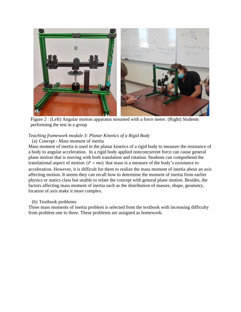
Figure 2 : (Left) Angular motion apparatus mounted with a force meter. (Right) Students

performing the test in a group

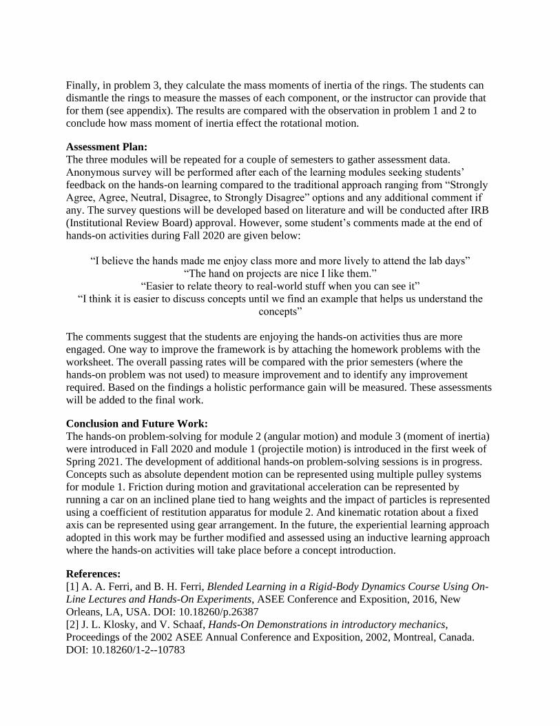
Teaching framework module 3: Planar Kinetics of a Rigid Body

(a) Concept - Mass moment of inertia

Mass moment of inertia is used in the planar kinetics of a rigid body to measure the resistance of

a body to angular acceleration. In a rigid body applied nonconcurrent force can cause general

plane motion that is moving with both translation and rotation. Students can comprehend the

translational aspect of motion ( )F ma= that mass is a measure of the body’s resistance to

acceleration. However, it is difficult for them to realize the mass moment of inertia about an axis

affecting motion. It seems they can recall how to determine the moment of inertia from earlier

physics or statics class but unable to relate the concept with general plane motion. Besides, the

factors affecting mass moment of inertia such as the distribution of masses, shape, geometry,

location of axis make it more complex.

(b) Textbook problems:

Three mass moments of inertia problem is selected from the textbook with increasing difficulty

from problem one to three. These problems are assigned as homework.

Table 7: Selected textbook problems for the moment of inertia [22]

Moment of inertia problem 1:

Given: mass of the ring 10 kg and each

slender rod 2 kg.

Find: find the moment of inertia about a

perpendicular axis passing through point A?

Moment of inertia problem 2:

Given: mass of the large ring, small ring, and

spokes are given.

Find: find the moment of inertia about a

perpendicular axis passing through point A?

Moment of inertia problem 3:

Given: mass per unit area is 20kg/m2.

Find: find the moment of inertia about a

perpendicular axis passing through point O?

(c) Representative physical model

A hands-on problem solving is developed to facilitate better comprehension of the moment of

inertia concept. Three problems are included in the lab session. The description of the problems

is given below, and the laboratory handout is provided in the appendix section.

(d) Model-problem:

Problem 1: Inertia

Experiential learning:

A set of two wands are used to experience inertia shown in Figure 3 (a). One is of the thick

aluminum shaft and the other one is thin with a movable mass. Students are asked to hold the

two wands in their hands and move up and down, changing the motion of the wands and note

their experience, which one requires more force Figure 3 (b). Next, they move the movable mass

outward and again note their experience. Afterward, the instructor explains that the masses of

both wands are the same and the resistance that the student feels during up & down motion is

inertia.

Figure 3: Set of two equal mass wands, one is of the uniform shaft and the other one is a thin

rod with movable mass.

Figure 4: Set of rings of equal mass, one with uniform shaft and the second one has a thin rod

with movable mass. Different moments of inertia cause the rings of equal mass to travel at a

different speed.

Problem 2: Moment of Inertia

Once students are clear about the inertia, next, they are given two rings; one with a uniform shaft

and the other one has a thin rod with a movable mass as shown in Figure 4 (left). Students are

asked to roll freely both ring down an inclined plane (a) the movable masses are near the center

and (b) the movable mass are near the rim. Students observe that though both rings are of the

same masses, the travel time is different Figure 4 (right). They can observe the effect of mass

distribution over the moment of inertia.

Finally, in problem 3, they calculate the mass moments of inertia of the rings. The students can

dismantle the rings to measure the masses of each component, or the instructor can provide that

for them (see appendix). The results are compared with the observation in problem 1 and 2 to

conclude how mass moment of inertia effect the rotational motion.

Assessment Plan:

The three modules will be repeated for a couple of semesters to gather assessment data.

Anonymous survey will be performed after each of the learning modules seeking students’

feedback on the hands-on learning compared to the traditional approach ranging from “Strongly

Agree, Agree, Neutral, Disagree, to Strongly Disagree” options and any additional comment if

any. The survey questions will be developed based on literature and will be conducted after IRB

(Institutional Review Board) approval. However, some student’s comments made at the end of

hands-on activities during Fall 2020 are given below:

“I believe the hands made me enjoy class more and more lively to attend the lab days”

“The hand on projects are nice I like them.”

“Easier to relate theory to real-world stuff when you can see it”

“I think it is easier to discuss concepts until we find an example that helps us understand the

concepts”

The comments suggest that the students are enjoying the hands-on activities thus are more

engaged. One way to improve the framework is by attaching the homework problems with the

worksheet. The overall passing rates will be compared with the prior semesters (where the

hands-on problem was not used) to measure improvement and to identify any improvement

required. Based on the findings a holistic performance gain will be measured. These assessments

will be added to the final work.

Conclusion and Future Work:

The hands-on problem-solving for module 2 (angular motion) and module 3 (moment of inertia)

were introduced in Fall 2020 and module 1 (projectile motion) is introduced in the first week of

Spring 2021. The development of additional hands-on problem-solving sessions is in progress.

Concepts such as absolute dependent motion can be represented using multiple pulley systems

for module 1. Friction during motion and gravitational acceleration can be represented by

running a car on an inclined plane tied to hang weights and the impact of particles is represented

using a coefficient of restitution apparatus for module 2. And kinematic rotation about a fixed

axis can be represented using gear arrangement. In the future, the experiential learning approach

adopted in this work may be further modified and assessed using an inductive learning approach

where the hands-on activities will take place before a concept introduction.

References:

[1] A. A. Ferri, and B. H. Ferri, Blended Learning in a Rigid-Body Dynamics Course Using On-

Line Lectures and Hands-On Experiments, ASEE Conference and Exposition, 2016, New

Orleans, LA, USA. DOI: 10.18260/p.26387

[2] J. L. Klosky, and V. Schaaf, Hands-On Demonstrations in introductory mechanics,

Proceedings of the 2002 ASEE Annual Conference and Exposition, 2002, Montreal, Canada.

DOI: 10.18260/1-2--10783

[3] S. Kaul, and P. Sitaram, Curriculum Design of Statics And Dynamics: An Integrated

Scaffolding And Hands-On Approach, In Proceedings of the 120th ASEE Annual Conference,

2013, Atlanta, Georgia. DOI:10.18260/1-2--19370

[4] J. Kadlowec, P. Von Lockette, E. Constans, B. Sukumaran, and D. Cleary, Hands-on

learning tools for engineering mechanics, Proceedings of the 2002 ASEE Annual Conference

and Exposition, 2002, Montreal, Canada. DOI: 10.18260/1-2--10616

[5] C. D. Pionke, J. R. Parsons, J. E. Seat, F. E. Weber, and D. C. Yoder, Integration of statics

and particle dynamics in a hands-on project-oriented environment, ASEE Annual Conference

and Exposition,1999, Charlotte, North Carolina. Available: https://www.jee.org/7767

[6] P. Avitabile, C. Goodman, J. Hodgkins, K. White, T. Van Zandt, G. S. Hilaire, and N.

Wirkkala, Dynamic systems teaching enhancement using a laboratory-based hands-on project,

In Proceedings of the 2004 ASEE Annual Conference, 2004, Salt Lake City, Utah. DOI:

10.18260/1-2--13872

[7] P. Avitabile, T. Van Zandt, J. Hodgkins, and N. Wirkkala, Dynamic systems teaching

enhancement using a laboratory-based project (RUBE), In Proceedings of 2006 ASEE Annual

Conference, 2006, Chicago, Illinois. DOI: 10.18260/1-2--414

[8] B. P. Self, J. Widmann, M. J. Prince, J. and Georgette, Inquiry-based learning activities in

dynamics, In Proceedings of the 2013 ASEE Annual Conference and Exposition, 2013, Atlanta,

Georgia. 10.18260/1-2--19775

[9] D. A. Kolb, Experiential learning: Experience as the source of learning and development, FT

press, 2014.

[10] T. Nakazawa, M. Matsubara, S. Mita, and K. Saitou, “Teaching materials and lesson plans

for hands-on mechanics education,” Experimental Techniques, Society, of Experimental

Mechanics, vol. 38(6), pp. 72-80, 2014.

[11] J. Vernon, C. J. Finelli, N. C. Perkins, and B. G. Orr, Piloting i-Newton for the experiential

learning of dynamics, In Proceedings of the 2015 American Society of Engineering Education

Annual Conference and Exposition, 2015, Seattle, Washington. DOI: 10.18260/p.24565.

[12] D. C. Yoder, J. R. Parsons, C. D. Pionke, and F. Weber, Hands-on teaching of engineering

fundamentals, Paper presented at 1998 Annual Conference, Seattle, 1998, Washington. DOI:

10.18260/1-2--7157.

[13] J. Bernhard, Teaching engineering mechanics courses using active engagement methods,

In Physics Teaching in Engineering Education (PTEE 2000), 13-17 June 2000, Budapest,

Hungary.

[14] F. A. Bella, The Trebuchet Project: Launching a “Hands-On” Engineering Technology

Approach To Conducting Hands-On Statics and Dynamics Laboratory Courses, ASEE Annual

Conference and Exposition, 2004, Salt Lake City, Utah. DOI: 10.18260/1-2--12865

[15] J. A. Kypuros, H. Vazquez, C. Tarawneh, and R. R. Wrinkle, Guided discovery modules for

statics and dynamics, ASEE Annual Conference and Exposition, 2011, Vancouver, BC. DOI:

10.18260/1-2—18043

[16]B. R. Campbell, L. E. Monterrubio, Laboratory Development for Dynamic Systems Through

the Use of Low-Cost Materials and Toys, ASEE Annual Conference & Exposition, 2014,

Indianapolis, Indiana. DOI: 10.18260/1-2--20730.

[17] B. S. Sridhara, Course-related undergraduate projects for dynamics, In ASEE Annual

Conference and Exposition, 2013, Atlanta, Georgia. DOI: 10.18260/1-2--19359

[18] A. Osta, and J. Kadlowec, Hands-on project strategy for effective learning and team

performance in an accelerated engineering dynamics course, In ASEE Annual Conference and

Exposition, 2016, New Orleans, Louisiana. DOI: 10.18260/p.25444

[19] B. Self, J. Widmann, G. Adam, Increasing conceptual understanding and student

motivation in undergraduate dynamics using inquiry-based learning activities, In ASEE Annual

Conference and Exposition, 2016, New Orleans, Louisiana. DOI: 10.18260/p.25668

[20] B. P. Self, and J. M. Widmann, Demo or hands-on? A crossover study on the most effective

implementation strategy for inquiry-based learning activities, In ASEE Annual Conference and

Exposition, 2017, Columbus, OH. DOI: 10.18260/1-2—28101

[21] A. Bao, Active Learning in Dynamics: Hands-on Shake Table Testing, Paper presented at

2020 St. Lawrence Section Meeting, 2020, Rochester, NY. Available:

https://strategy.asee.org/33895

[22] R. C. Hibbler, Engineering Mechanics: Dynamics, 14th Edition, Hoboken, New Jersey:

Pearson Prentice Hall, Pearson Education, Inc. 2016.

[23] Xpult catapults.

https://www.xpult.com/?gclid=Cj0KCQjwgtWDBhDZARIsADEKwgP8vVQuJKC1QokjIbVnQ

XwOOqalyrlpKLFcBVifGAkxpzmKxDR3QMEaAoBUEALw_wcB

[24] Vernier Centripetal force apparatus. https://www.vernier.com/product/centripetal-force-

apparatus/

[25] Newton spring scale, https://www.fishersci.com/shop/products/clear-plastic-spring-scales-

4/p-7199126#?keyword=spring%20scale

[26] Science first moment of inertia apparatus. https://shop.sciencefirst.com/force-

equilibrium/3979-moment-of-inertia.html

Acknowledgment:

The physical models are purchased using a faculty development mini-grant 2020, Angelo State

University.

Appendix:

Lab: Inertia and Moment of Inertia

Problem 1: Inertia

LO: To be able to identify inertia and be able to relate inertia with real world

Given the two wands, one is of the thick aluminum shaft and the other one is thin with

movable mass.

(a) Secure the movable mass to the handle of the thin wand. Pick up the wand using one

hand and use the other hand to pick up the thick aluminum wand. Now compare and

write down which one is heavier.

Answer: The heavier wand is the ……………………………………..

(b) Next, slide the movable mass (brass weight) opposite the end of the thin wand. Pick up

the wand using one hand and use the other hand to pick up the thick aluminum wand.

Now compare and write down which one is heavier.

Answer: The heavier wand is the ……………………………………..

(c) Did you see any discrepancy in your results of (a) and (b)? Explain with an example of

a lever system why do the wands behave like this?

(d) While comparing the wands in your hands you move your hands up and down and

changing the motion of the wands. The resistance you feel is the inertia of the wands.

The tendency of an object to resist changes in its state of motion varies with mass. The

more mass that an object has, the more inertia that it has. However, if the mass of the

two wands is the same, why one wand felt heavier than the other?

(e) Considering the above observation and recall the concept of inertia that is a moving

object will continue to move in the same direction & velocity, and an object at rest will

stay at rest unless an unbalanced force is applied. Explain what do you think of

whether a force is required or not to keep an object moving?

Problem 2: Moment of Inertia/ Rotational inertia/ Angular mass

LO: To be able to describe the moment of inertia and be able to relate moment of inertia with

real world

Given the two rings, one with a thick bar and the other one is with movable masses. Set up an

inclined plane of 1 m length at a 30-degree angle and grab a stopwatch.

Items needed: ruler, stopwatch, inclined plane, support to have 30 degree

(a) Place the ring with a thick bar at the top on the inclined plane and allow it to roll

freely down the plane and measure the required time. Take at least three data.

Answer: Required time ………………..

(b) Take the other ring and push both movable masses into the center of the ring. Place the

ring at the top on the inclined plane and allow it to roll freely down the plane and

measure the required time. Take at least three data.

Answer: Required time …………………

(c) Next, push both movable masses to the outer rim of the ring. Place the ring at the top

on the inclined plane and allow it to roll freely down the plane and measure the

required time. Take at least three data.

Answer: Required time …………………

(d) Compare the required travel times of the rings and discuss which ring (whether thick or

thin) is heavier?

(e) What causes the time difference between test (b) and (c) since it is the same ring with

different mass distribution?

(f) If both rings are of equivalent mass what causes the change in the required time?

Problem 3: Determine the Moment of Inertia

LO: To be able to recognize and solve angular motion problems and find

normal components of acceleration and force (See assigned homework)

Calculate the moment of inertia of both rings about the ground (i.e. point

A). For the ring with movable mass; consider two scenarios (the masses are

at the out end of the rim, the masses are moved to the center of the rim).

Total three Moment of Inertia for three groups (one per each).

Measure the dimensions and mass of the rings:

• Thick-bar ring:

✓ Ring: 116.26 gm

✓ 2 screw: 2.87 gm

✓ Aluminum bar: 205.01 gm

✓ Ring inner dia.: 15 cm, outer dia.:

16 cm

Bar length: 14.6 cm

• Thin-bar ring:

✓ Ring: 118.47 gm

✓ 2 screw: 2.86 gm

✓ Cylindrical mass: 100.61 gm each

Each cylinder: 2.5 cm long, dia: 2.5 cm

Analyze your results and answer the following:

I. (True/False) The moment of Inertia depends on mass distribution around the axis about

which the moment of inertia is calculated.

II. Explain comparing the results why the three cases have different travel times while the

total mass is the same?

Note: Split the class into two groups. Problem 1 and 2 will be assigned to the two groups.

Which should take about 10 minutes. Next, allow 5 minutes for each group to explain the

solutions to the other group (the other group can ask questions). The last 30 minutes will be

dedicated to Problem 3 problem-solving. Split the class into three groups (one Moment of

Inertia or each group) though the dimensions are provided students will have access to the

physical model if needed.