r~3 HEWLETT~r. PACKARD

Work Notes on Elementary Matrices

Augustin A. DubrulleComputer Systems LaboratoryHPL-93-69July, 1993

dubrulle@hpl.hp.com

matrixcomputations,matrix blockalgorithms, linearalgebra

Elementary matrices are studied in a generalframework where the Gauss and Householdertypes are particular cases. This compendiumincludes an analysis of characteristic properties,some new derivations for the representation ofproducts, and selected applications. It is thecondensation of notes useful for the developmentand test of matrix software, including high­performance block algorithms.

© Copyright Hewlett-Packard Company 1993

Internal Accession Date Only

Work Notes on

ELEMENTARY MATRICES

AUGUSTIN A. DUBRULLEHewlett-Packard Laboratories

1501 Page Mill RoadPalo Alto, CA 94904

dubrulleGhpl.hp.com

July 1993

ABSTRACT

Elementary matrices are studied in a general framework where theGauss and Householder types are particular cases. This compendiumincludes an analysis of characteristic properties, some new derivationsfor the representation of products, and selected applications. It is thecondensation of notes useful for the development and test of matrixsoftware, including high-performance block algorithms.

1 Introduction

Elementary transformations [7, 8, 13] are the basic building blocks of nu­merical linear algebra. The most useful transformations for the solutionof linear equations and eigenvalue problems are represented by two typesof elementary matrices. Householder matrices (or reflectors), which con­stitute the first type, preserve the euclidean norm and are unconditionallystable. Gauss matrices, which make up the second type, are economical ofcomputation, but are not generally stable. The product of a Gauss matrixand a well-chosen, data-dependent, transposition matrix (another elemen­tary matrix) defines a transformation the instability of which is contained,and which sometimes constitutes a practical alternative to Householder re­flections. Such "stabilized" elementary transformations are the basis foralgorithms using techniques of pivoting in the solution of linear equationsand eigenvalue problems [13].

Real Householder and Gauss transformations are members of a largerclass represented by the generic matrix

T = I+vwT,

1

(1.1)

where the vectors v and ware arbitrary. Typically, elementary transfor­mations are used for the annihilation of selected elements of a vector or amatrix. The transformation of a nonzero vector

y=Tx, x f=. 0,

.' defines T from equation (1.1) by the following relations:

y-xv=-T-'wx

The elementary matrix so specified is not unique, and additional constraintshave to be placed on w to lift the uncertainty. Yet, selected components ofx can be annihilated by T with

i E I.

Conversely, the components of x corresponding to null components of v areinvariant under T:

Vj = 0 {:} Yj = Xj, j E:T.

These features have made the elementary matrix a powerful instrument ofalgorithm design and implementation. This report is a repertory of proper­ties, formulas, and other information useful for the development of matrixsoftware. Some of the material is new or hitherto unpublished.

2 Basics

We first derive some simple norms. Starting with the basic expressions

we get

(2.1)

The inverse of an elementary matrix, if it exists, is another elementary matrixdefined by

for which we have the norms

-1 T'Y- +w v, (2.2)

2

Condition numbers for the above norms are obtained from equations (2.1),(2.3),and the definition

A transformation is involutory if it coincides with its inverse. Fromequations (1.1) and (2.2), an elementary matrix is involutory if 'Y = -1, thatis,

T = T-1 {:} wTv = -2.

Using the property that the inverse and the transpose of an orthogonalmatrix are equal, we derive the condition for an elementary matrix to beorthogonal,

TT = T-1 {:} w = -2I1vll-2v,

where 11.11 designates the i 2(n) norm 11.112. Orthogonal elementary matricesare Householder reflectors, which are symmetric and involutory:

H =1+ auuT,

The Householder transformation Hi, that annihilates all components of avector x other than x k,

1,131 = II x ll,

is specified by

u = x - ,l3ek,

For implementation purposes, this matrix is often expressed in the followingequivalent forms,

1 THj, = 1+ -vv ,Vk

Hk =1+ VkwwT,

1w=-v,

Vk

where the vectors are normalized for trouble-free computation.A transposition matrix is a particular reflector defined by

Sk,m =1- (ek - em)(ek - emf,which exchanges the kt h and mth components of a vector.

Gauss (or Jordan) matrices are defined by the choice of a vector of thecanonical basis for w:

3

The most common use for a Gauss (or Jordan) matrix! is to annihilate allthe components of a vector x other than Xk, Xk =f 0:

For that matrix, l' = 1, and the inverse satisfies

Gk"l =1 - vef, that is, Gk +Gk"l = 21.

There is another type of Gauss matrix,

- - Tc, = I+vek,

which also reduces x to a stretching of ek. It is involutory, and is defined by_ xv = -ek --.

Xk

Note that, for a same vector x, the vectors v and v of Gk and G k differonly by their k th components. While the effects on x of Gk and Gk are verymuch the same in most practical applications (the sign change in the resultis seldom important), these two matrices have a fundamental difference thatwe shall discuss later. Although Gk is computationally equivalent to Gk formost algorithms, it is never used in practice.

From equations (2.1) and (2.3), we get the norms

p = 1,00.

For a same vector x, the corresponding fl(n) and foo(n) norms of Gk andGk take the same values. These matrices also have the same norms as theirinverses.

The transformation defined by the pairing

i = 1,2, ... , n,

is the basic operation of Gaussian elimination methods using partial piv­oting. It is referred to as a stabilized elementary transformation [13], asthe components of the vector v generated for Gk by 0k,mX are bounded byunity. A stabilized elementary transformation can be similarly built from aninvolutory Gauss matrix, but it must be noted that the product Gk8k,m isnot necessarily involutory. In the following, we refer to a Gauss matrix asstabilized if its associated v vector is bounded by unity in the infinity norm.

lSome authors [7] distinguish between Gauss and Jordan elementary matrices as follows:(1) a Jordan transformation annihilates the elements of a vector other than a designatedelement, and (2) a Gauss transformation annihilates the elements of a vector below aspecified element. For simplicity, noting that a Gauss transformation coincides with aJordan transformation in a subspace, we do not make such a distinction, and we use theappellation "Gauss matrix" for either type.

4

3 Proper and singular elements

We first look at the proper vectors and values of T. We note that thesubspace P orthogonal to w is an invariant subspace of dimension (n - 1)for the proper value unity:

We also have

Tx = x ¢} x E P, P 1. w.

Tv =,v.If v is not in P, v and P define a full set of proper vectors associated withthe proper values, and unity, the latter with multiplicity n - 1. This caseis exemplified by the matrices Hk and Gk of the previous section. If v is inP, , = 1, and T is defective: all the proper values are unity, and there areonly (n - 1) proper vectors. The above Gauss matrix Gk is of this type.

We now turn to the determination of the singular values and the rightsingular vectors. A singular vector x and the associated singular value (7

satisfy

(3.1)

where 11.11 denotes 11.112'We first assume that v and w are not collinear. Let S be the subspace

orthogonal to {v, w}. S is a singular subspace associated with (n - 2) unitsingular values, and any orthogonal basis of S forms a set of (n - 2) rightsingular vectors. Since neither of the two remaining right vectors can beparallel to v or w, we must have the generic representation

v wx = H + J.L IIwll ' (3.2)

to a scaling constant. Substituting this expression in equation (3.1) andseparating the terms in v and w, we get

(72 = , +J.LIIVIlIIWIl,

J.L(72 = 'J.L +,lIvllllwll +J.LllvIl 2I1 wIl2

•

The elimination of (72 from the second of these equations yields

(3.3)

(3.4)

Using the Cauchy-Schwartz inequality, it is easy to show that the discrimi­nant of this quadratic equation in J.L is non-negative. The roots are

J.L2 = _.2..,J.LI

5

which define the two right singular vectors Xl and X2 by formula (3.2). Thedetermination of the associated singular values immediately follows. Fromequations (3.4) and (3.3), we have

after taking a square root. Hence, the nonunit singular values

are associated with the (unnormalized) right singular vectors

v WX2 = IIvll - sgn(-Y)0"2

I1 w ll'

Using the squares ofthe singular values and the Cauchy-Schwartz inequality,it can be shown that 0"1 and 0"2 are the extreme singular values:

The corresponding (unnormalized) left singular vectors Yl and Y2 are definedby the basic equation

which yields

v W

Yl = O"lllvil + IIwll'

The other left singular vectors coincide with their right homologues in thesubspace S orthogonal to {v, w}. Since 0"1 and 0"2 are the extreme singularvalues, we have

or (T) _ / + O"lllvllllwilK,2 - 1,1 .

When v and ware collinear,

w=pv,

and S reduces to the subspace orthogonal to v. Any orthonormal basis of Sis a set of (n - 1) right (and left) singular vectors for the singular value unitywith corresponding multiplicity. The remaining singular value and vectorsare

V

xi = IIvll'

6

The Householder reflector is in that class of matrices, with 'Y = -l.From the above, we get the nonunit singular values and condition number

of the Gauss matrix Gk for w =ek and 'Y = 1:

Identical results are obtained for the involutory Gauss matrix Gk. Fromhere, it is easy to show that the l2(n) condition number of a stabilizedGauss transformation is bounded by (n + 1).

4 The Bischof-Van Loan expressions of products

Most methods for the numerical solution of the standard problems of linearalgebra rely on sequences of elementary transformations to reduce a matrixto some special form. In a serial implementation of these methods, r trans­formations cause some elements of the matrix to be fetched and stored r

times. Since the processing times of memory references and arithmetic oper­ations are about the same for high-performance computers, much effort hasbeen devoted to reducing the occurrence of the former for better efficiency.One successful approach to that end consists of representing a sequence of r

elementary transformations by a single operator, which, when applied to amatrix, generates substantially fewer than r memory references per matrixelement. The construction of that operator may create some computationaloverhead that can be controlled by the value assigned to r. Algorithms usingthat device are the basis for the design of recent high-performance libraries[1]. They are rich of matrix operations, and are often referred to as blockalgorithms. The derivations below follow the work by Bischof and Van Loan(B-VL) on the representation of products of Householder matrices [2].

Consider the product of r elementary matrices of order m with r < m,

Tk = I+VkWr,

where Vi and w, can be arbitrary. We show that any such product can beexpressed in the form

p(k) = I +X(k)W(k)T,k

W(k) == LWi. (4.1)i=l

Noting that this representation is obvious for r = 1 with X(l) = vlef, letus assume that identity (4.1) is true, for which we have

7

This last equation immediately yields the expression

X(k+l) = (I +vkHwIH)x(k) +vkHelH,

which verifies the representation

Similarly, it can be proved that there exists a formula

(4.2)

p(r) = 1+v(r)y(r)T, V(k) y(k) E R mxk, ,k

V(k) =LVi,i=l

for which y(r) is defined by the recurrence

Y (l ) - w eT- 1 l'

This type of representation leads to block algorithms with the best timeperformance [5].

5 The Schreiber-Van Loan variants

The Schreiber-Van Loan (S-VL) representation is a modification of the B-VLexpression of products that trades the x(r) (or y(r») matrix for a triangularmatrix of order r and thereby leads to implementations more economical ofstorage.

Starting fromxV) = v· J" < k

J J' -,

the recurrence (4.2) generates the equations

i = j +1, ... ,k,

which, after summation with respect to i, yield

This expression reveals x}k) as a linear combination of {Vj,VjH, ... ,Vk},

and implies the existence of a lower-triangular matrix r(k) with unit diagonalsuch that

X(k) = v(k)r(k), r(k) E R kxk .

r(k) is the "middle matrix" of the Schreiber-Van Loan representation [11]

p(k) = I + v(k)r(k)w(k)T,

8

which is more economical of storage than the alternatives of the previoussection for the case of Householder matrices. The identity

readily generates the recurrence

r(j) = r(j-I) +ej (W;y(j-I)r(j-I) +en ' (5.1)

which can be used to build r(k) row by row, starting from r(l) = elef. Thisis the approach taken in [11] for the case of Householder matrices. Note thatequation (5.1) is equivalent to

r(j) = r(j-I) +ej (w;X(j-I) +en '

where X(j-I) is the matrix of the B-VL representation. This matrix, how­ever, does not have to be computed.

Dropping superscripts for simplicity, let

P = I+yrWT, y,W E n ffl x r,

represent the product of r elementary matrices. For k ~ r, any matrix r(k)of the previous section is a leading principal submatrix of I', while y(k) andW(k) derive from the restriction of Y and W to their leading k columns.Left multiplication of equation (5.1) bye; yields

j=1,2, ... ,r, (5.2)

that is, the lh row of r. In that equation, the term crucial to closed-formexpression is the vector

wTy(j-I)J '

for which we introduce the additive triangular decomposition

WTy=£+u, iij = 0, i ~ j. (5.3)

With this definition, we have

wTy(j-I) = eTcJ J '

for which equation (5.2) generates the matrix expression

r=I+£r

9

and the following closed fomr' of the middle matrix:

(5.4)

Still making no particular assumption about Y and W other than 1+ U benot singular, we now derive the inverse of

(5.5)

The Sherman-Morrison formula applied to P in its original form yields

in which we use the decomposition (5.3) to get

(5.6)

an expression similar in form to that of equation (5.5).We now briefly consider the particular case of Householder matrices,

j = 1,2, ... ,r,

which we recast in the form

W = YD-I ,

The representation of the product reduces to

a =Dr-I, (5.7)

where a is lower-triangular. Using the orthogonality property of P and theexpression (5.6) of the inverse, we get the relation

a+aT = -vtv, (5.8)

which provides the algorithm for the computation of a from Y alone.The representation of the middle matrix by its inverse I-£' has inter­

esting computational implications that we explore below. The constructionof I' with the recurrence (5.1) requires about

2This expression was independently developed by Puglisi [10] for Householder matrices.

10

floating-point operations, while the computation of r- 1 with formula (5.4)takes

h ~mr2

operations. The difference in those numbers reflects the fact that the re­currence (5.1) actually combines the computation of r-1 and its inversion,as

r 3

ft-h~-3

is about the number of operations required for the inversion of a triangu­lar matrix of order r. Under the reasonable assumption that multiplicationby a lower-triangular matrix requires the same amount of work and machinetime as the multiplication by the inverse (a simple forward substitution), theimplementation of block methods based on the S-VL representation shouldbenefit from using r-1 instead of r. At each block step of the QR factoriza­tion of a matrix of order n with blocking parameter r, r 3 /3operations can beavoided, for an approximate total saving of nr2 /3floating-point operations.What is more important is that the construction of £ can be carried outwith some level-3 BLAS for the rank-r update of a symmetric matrix.

6 Remarks on implementation

Implementations of elementary transformations (and products thereof) forhigh-performance machines are far from being uniquely defined, even withthe use of tuned BLAS [9, 3, 4]. In this section, we briefly review some ofthe possible choices with a definite bias for fast scalar architectures withhierarchical storage (including a cache). The focus is on Householder ma­trices, which are computationally more complex than their Gauss relatives.To limit the scope of the discussion, we exclude the cases where the trans­formations have small dimensions (e.g., plane reflections, or transformationsof dimension three of the LR or QR algorithms for real Hessenberg matri­ces). Likewise, the assumption that the fast memory (proximal cache) canaccomodate more than just a few columns of the matrix being transformedeliminates the case of very large dimensions. Questions of stride of referenceto the matrix elements assume a FORTRAN organization of two-dimensionalarrays in which consecutive elements of a column are stored in contiguousmemory cells. Parentheses in equations below indicate computational blocksand order of operation.

We start with the left multiplication of a matrix A E R n x n by an ele­mentary matrix,

(6.1)

11

which, in this form, can be considered as a rank-I update of A. A naturalway to organize the computation is based on a partition of the matrix instrips of s columns (perhaps fewer for the last strip) such that a strip can becontained in the cache. As soon as the segment of w T A corresponding to astrip is computed, it can be used for the update of the strip, which at thatpoint may be overwritten in storage (in situ transformation). Computingand keeping the segment in s registers (the accumulators of the scalar prod­ucts) for immediate use in the matrix update minimizes storage referencesand efficiently exploits the data present in the fast memory. The determi­nation of the optimum value of s usually requires further information onmachine architecture. Note that a finer performance analysis of this compu­tation is likely to require some additional partitioning of the matrix for theefficient calculation of each segment of w T A (this remark in fact applies toall the transformations considered in this section). We shall not discuss thislevel of detail, which is usually handled by some efficient BLAS - or in-linesubstitute code.

Using a similar approach, and assuming that the cache can hold s rowsof A, we express the right multiplication by

which suggests for A a partitioning in strips of s rows, with a correspond­ing computation of Aw segment by segment. As each segment becomesavailable, it can be used for the update of the associated matrix strip.

The elementary orthogonal similarity transformation of a matrix,

naturally lends itself to a wider variety of algorithms. The first consists of asequence of two one-sided transformations,

B = A + (Aw)vT, (6.2)

which is entirely executed by level-2 (matrix-vector) operations. Anotheralgorithm expresses the transformation as two combined matrix updates ofrank one:

C = A + vfT +gvT,

f = ATw+! (wTAW) v, g = Aw+! (wTAw) v.

In general, this scheme is not as efficient as the one prescribed by equation(6.2), as the construction of f and g requires level-1 (vector) operations,

12

namely, one scalar product and two elementary linear combinations. WhenA is symmetric, however, the equality of f and g reduces complexity, andsymmetry can be preserved throughout the computation.

While the use of BLAS in the implementation of these operations isbeneficial, it prevents the kind of optimization outlined for the left trans­formation (6.1), where the registers containing partial results of Awareimmediately used for the update of a strip of matrix. At best, for re-useof the cache contents (a strip of matrix), stripping can be made an explicitpart of the program performing the operation, and the BLAS for matrix­vector multiplication and matrix update can be called in sequence for eachstrip. We do not consider this approach to be satisfactory, and not becauseof the minor performance loss due to nonoptimal use of registers. What ismore serious is the burden placed on the user for some optimization thatcan be better achieved with tuned subprograms implementing Householdertransformations. Such software, which is included in LAPACK in the formof obscure auxiliary routines (the _LARF_ set), fully deserves inclusion inthe BLAS.

The above comments carryover to products of Householder transforma­tions, for which best performance is achieved with B-VL representations.This level of efficiency is matched by the S-VL representation for one-sidedtransformations only if modified to use the inverse of the middle matrix(5.7) and the construction (5.8) . For similarity transformations, the B-VLimplementation is still slightly faster. The construction of its x(r) or y(r)

matrices (Section 4) is best performed by using the inverse I-£. or .6.-1

of the S-VL middle matrix and appropriate level-3 BLAS. In the following,we outline sample implementations of block methods that illustrate thesepoints (the operations are expressed for execution by level-3 BLAS).

Let Y be the matrix in R n x r whose columns are vectors associated witha sequence of Householder transformations. Using formula (5.8), .6. is con­structed by forming the lower-triangular part of - vtv and multiplying itsdiagonal by one half. These two matrices define the matrix of the productof the transformations:

P =1+ Y.6.-1y T ,

which we apply to a matrix A. We first consider the case of a left transfor­mation in situ,

A:=PA,

for which the S-VL implementation requires an ancillary array of (r X n)

13

cells for the intermediate matrices represented by Z:

Z:= ATV,

Z:=Z.o.-T,

A:=A+VZT •

(forward substitution)

Two arrays of (r X n) cells are needed for the intermediate matrices Y andZ in the B-VL implementation below:

Y:= V.o.-T,

Z:= ATy,

A:=A+VZT •

(forward substitution)

It is clear that the additional expense of storage for Y matrix of the the B­VL representation cannot be justified, since the two schemes differ only bythe order of operation. The same comment applies to right-hand transfor­mations. Hence, the S-VL implementation should be preferred for one-sidedtransformations.

The case of a similarity transformation

is somewhat different. Its S-VL implementation is represented by:

Z:=AV,

Z:= Z.o.-T,

A:=A+ZVT ,

Z:= ATV,

Z := Z.o.-T,

A:=A+VZT•

(forward substitution)

(forward substitution)

Note that this procedure uses only one ancillary array and performs twoforward substitutions. The B-VL approach uses two arrays and performs

14

only one forward substitution:

Z:=AV,

Y:= V.:l-1 ,

A:=A+ZyT,

Z:= ATV,

A:= A+YZT.

(forward substitution)

The gain in performance is very slight if r is a small fraction of n, a condi­tion usually satisfied in practice. This consideration should make the S-VLscheme based on the inverse of the middle matrix the preferred design forlibrary software".

7 Transformations in two dimensions

Transformations in two dimensions commonly appear in larger computationssuch as the solutions of standard and generalized eigenvalue problems, fromwhich the instances discussed below are borrowed.

We first consider orthogonal transformations. In most applications, theseare practically interchangeable with Givens rotations [7] represented by thematrix

which is not of the Householder type (it is the product of a Householdertransformation and a transposition). While reflectors in two dimensions canbe used in the general form of Section 2

H =1- 2uuT,

they can also be represented by

H=[C s]s -c '

lIuli = 1,

(7.1)

The equivalence of the two representations follows from letting Ul and U2 bethe sine and cosine of an arc, which defines s and C of equations (7.1) as thesine and the cosine of the double arc. A matrix (7.1) is usually referred toas a plane reflector or a Givens reflector.

3The current S-VL implementations in LAPACK do not use the inverse of the middlematrix, more likely by an accident of timing rather than by design.

15

The simplest use of a Givens reflector is found in the annihilation of acomponent of a vector, as illustrated by the transformation

which, as for a plane rotation, defines

A more complicated problem is the similarity reduction of a matrix A oforder two to some special form B:

[e s] [aus -e a2l

(7.2)

Assuming that e =J °and letting

1e - ---===- JI+t2' s = te,

we transform equation (7.2) into the equivalent form

a2lt2 +dt - a12 ]

allt2 - et + a22 •(7.3)

This expression is the basis for the derivation of special transformations, in­cluding the reduction of A to standard upper Schur form, which we considernow. The standard Schur form B of A is defined as follows: if A has realeigenvalues, B is upper-triangular, while if A has complex eigenvalues, blland b22 are equal and coincide with the common real part of the eigenvalues.Assuming that a2l =J 0, we first handle the simple case a12 = 0, for which theassignments c =°and s = 1 produce the desired result through an exchangeof the rows and columns of A. In the general case, the condition b21 = 0and equation (7.3) lead to

(7.4)

This equation has real roots if

6 ~ 0,

As expected, this is the condition for which A has real eigenvalues. It iseasy to check that the simple change of variable

16

tranforms equation (7.4) into A's characteristic equation. Instead of solvingequation (7.4) to determine the reflection that triangularizes A (when itexists), it is numerically better to perform (1) a similarity reflection thatproduces a matrix with equal diagonal elements, followed by (2) a similarityreflection that triangularizes that matrix when the eigenvalues are real. Thistechnique is used by the LAPACK auxiliary routine -LANV2 for a reductionto Schur form by plane rotations. Some of the reasons for the preferablilityof this approach are easily seen in equation (7.3). In the following, we treatthe two phases of the above computation as two separate problems.

From equation (7.3), the reflection for which bll = b22 is defined by

d t2- 2e t - d = 0 d# O.

This equation has real roots since its discriminant ~ is always positive,

Choosing the root of smaller magnitude to maximize c,

dt = -sgn(e) ~'lel+ ~

we obtain the formulas

_ 1 ( lei )1/2C-J2 1+~ ,

which prescribe safe computations for the solution of our first problem.For the second problem, we use again equation (7.3) with the assumptions

for which the triangularization formulas reduce to

_f¥12c- -,e

s= Ja;1,In principle, the problem of similarity triangularization can also be solved

with the use of Gauss transformationsv, albeit not as satisfactorily from aviewpoint of numerical stability. We briefly look at such an approach in theremaining part of this section.

4Such a triangularization is no longer a reduction to Schur form since Gauss transfor­mations are not orthogonal.

17

To parallel the above discussion, we consider the similarity transforma­tion of A by an involutory Gauss matrix,

[~ _~ ] [:~~ :~:] [~ _~ ] = [:~~ :~:], (7.5)

which leads to the expression

B = [ a1292+au -a12 ]

d,d = au - a22· (7.6)

a129 + 9 - a21 -a129 +a22

Predictably, the triangularization of A is predicated on the existence of areal solution 9 of the same equation as in the orthogonal case (7.4):

a1292 +d9 - a21 = 0,

If real roots exist, the root of smaller magnitude should be chosen to mini­mize the condition of the elementary matrix (see Section 3):

2a219 = sgn(d) Vi'Idl + c

c~ O.

In addition, the elementary matrix will be stabilized under the followingcondition,

la211 s la121 ::} 191 ::; 1,

which can be proved using the inequality C~ O.When the eigenvalues of A are complex, the specification bu = b22 is

realized with

d9 = ---,

2a12s< 0,

Finally, triangularization in the case where ail = a22 leads to

{!!;21g= -,a12

to which the usual stability condition applies. To satisfy this condition, asimilarity transposition may be needed first to bring the off-diagonal elementof smaller absolute value into sub-diagonal position. Preferably, this effectis achieved in practice by explicitly exchanging the columns of the Gaussmatrix for the left transformation in equation (7.5), and by exchanging itsrows for the right transformation (the scrambled matrices are no longerinvolutory). The similarity transformation (7.6) then becomes

B = [_~ ~] A [i -~],

18

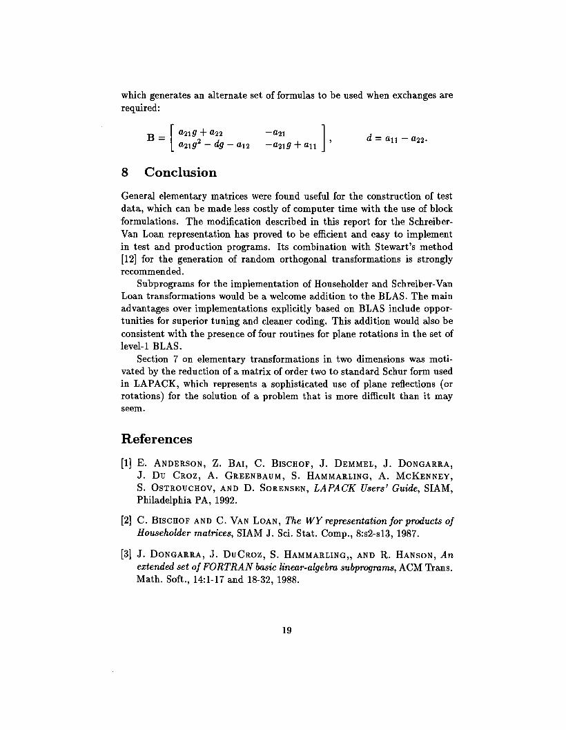
which generates an alternate set of formulas to be used when exchanges arerequired:

8 Conclusion

General elementary matrices were found useful for the construction of testdata, which can be made less costly of computer time with the use of blockformulations. The modification described in this report for the Schreiber­Van Loan representation has proved to be efficient and easy to implementin test and production programs. Its combination with Stewart's method[12] for the generation of random orthogonal transformations is stronglyrecommended.

Subprograms for the implementation of Householder and Schreiber-VanLoan transformations would be a welcome addition to the BLAS. The mainadvantages over implementations explicitly based on BLAS include oppor­tunities for superior tuning and cleaner coding. This addition would also beconsistent with the presence of four routines for plane rotations in the set oflevel-1 BLAS.

Section 7 on elementary transformations in two dimensions was moti­vated by the reduction of a matrix of order two to standard Schur form usedin LAPACK, which represents a sophisticated use of plane reflections (orrotations) for the solution of a problem that is more difficult than it mayseem.

References

[1] E. ANDERSON, Z. BAI, C. BISCHOF, J. DEMMEL, J. DONGARRA,J. Du CROZ, A. GREENBAUM, S. HAMMARLING, A. MCKENNEY,S. OSTROUCHOV, AND D. SORENSEN, LAPACK Users' Guide, SIAM,Philadelphia PA, 1992.

[2] C. BISCHOF AND C. VAN LOAN, The WY representation for products ofHouseholder matrices, SIAM J. Sci. Stat. Comp., 8:s2-s13, 1987.

[3] J. DONGARRA, J. DUCROZ, S. HAMMARLING" AND R. HANSON, Anextended set of FORTRAN basic linear-algebm subprogmms, ACM Trans.Math. Soft., 14:1-17 and 18-32, 1988.

19

[4] J. DONGARRA, J. DUCROZ, S. HAMMARLING" AND 1. DUFF, A set oflevel-S basic linear-algebra subprograms,ACM Trans. Math. Soft., 16:1-17and 18-28, 1988.

[5] A. DUBRULLE, On block Householder algorithms for the reduction of amatrix to Hessenberg form, in Sup ercomputing'88: Vol. II, Science andApplications, Martin and Lundstrom eds., IEEE Computer Society Press,Washington DC, 1989.

[6] A. DUBRULLE, On FORTRAN matrix software and vector computing,Proc. Third IMSL Users North America Conf., Monterey CA, 1990.

[7] G. H. GOLUB AND C. F. VAN LOAN, Matrix Computations, The JohnsHopkins University Press, Baltimore MD, 1989.

[8] A. S. HOUSEHOLDER, The Theory of Matrices in Numerical Analysis,Blaisdell, New York NY, 1964.

[9] C. LAWSON, R. HANSON, R. KINCAID, AND F. KROGH, Basic linear­algebra subprograms for FORTRAN usage, ACM Trans. Math. Soft.,5:308-323, 1979.

[10] C. PUGLISI, Modification of the Householder method based on the com­pact WY representation, SIAM J. Sci. Stat. Comp., 13:723-726, 1992.

[11] R. SCHREIBER AND C. VAN LOAN, A storage-efficient WY represen­tation for products of Householder transformations, SIAM J. Sci. Stat.Comp., 10:53-57, 1989.

[12] G. W. STEWART, The efficient generation of orthogonal matrices withan application to condition estimators, SIAM J. Num. Anal., 17:403-409,1980.

[13] J. H. WILKINSON, The Algebraic Eigenvalue Problem, Clarendon Press,Oxford, 1965.

20