workflows: attribute-assisted footprint suppression -...

Workflows: Attribute-Assisted Footprint Suppression

Attribute-Assisted Seismic Processing and Interpretation

ATTRIBUTE-ASSISTED FOOTPRINT SUPPRESSION – PROGRAMS kxky_prep, kxky_forward, generate_mask, kxky_reverse, AND

adaptive_subtraction

Acquisition footprint often poses a major problem for 3D seismic data interpretation. Ideally, footprint from acquisition is handled at the processing shop through more careful attention to trace balancing statics, noise reduction, and velocity

analysis (Hill et al., 1999; Gülünay, 2000). Such reprocessing is not feasible on many legacy data volumes where the pre-stack data cannot be found or no longer exists. Seismic attributes often provide an effective means of delineating subtle geological

features of interest such as channels, small faults, and fractures, but can also enhance acquisition footprint. For this reason attributes can be used to both design and evaluate the effectiveness of alternative footprint suppression workflows.

Computation flow chart for footprint suppression

The AASPI footprint suppression GUI is found under AASPI Workflows.



The footprint suppression tool is actually a processing workflow using kx-ky filters and adaptive subtraction. kx-ky filters are routinely used in the image processing industry to

remove periodic noise that contaminates medical images and maps. Filters can be

designed as a function of the wavenumber to remove coherent, periodic or aperiodic noise (Buttkus, 2000). The figure from Falconer and Marfurt (2006) shows the detailed workflow for this process.

Since we are addressing legacy post-stack data volumes, no source or receiver geometry information is retained in the headers. Therefore, the first step is to generate

footprint-contaminated attributes from the migrated seismic data. To estimate the noise, footprint is enhanced and stratigraphic signal suppressed by applying a vertical median filter that removes the stratigraphic features (1). Along with rescaling the attribute

amplitudes, a constant bias may need to be added to the attribute data to force noise-free (e.g. high coherence, c=1) values to be the same as null values in muted and dead trace zones. Once the footprint is enhanced, it is transformed to kx-ky space and smooth

pedestal filters are generated that best represent the acquisition footprint in the seismic attribute volume (2). Parallel to the footprint characterization steps described above, the seismic amplitude volume is transformed to kx-ky space and masked with the pedestal



filters generated from the attribute data(3). The reverse transform of the masked amplitude data yields modeled noise time or horizons slices (4 and 5) that are then adaptively subtracted from the original data to produce filtered seismic data (6). Finally

we unslice the filtered seismic data (7). Footprint sensitive attributes are computed from the filtered data to QC the filtering process and decide whether the data need more filtering or is ready for interpretation.

Step-by-Step Description of the Workflow The goal of the footprint suppression workflow is to generate an estimate of the footprint

noise component which will be subsequently subtracted from the original unfiltered data using a least-squares adaptive subtraction technique.



Step 1. Attributes often exacerbate the effects of acquisition footprint. The goal of step 1

is to first choose an attribute that enhances the footprint. If the footprint gives rise to anomalous amplitudes, then the total energy attribute may be a good choice. If we see

changes in apparent dip due to inaccurate velocities, a curvature attribute may work well. One of the first attributes to try is the Sobel filter similarity, which is sensitive to both lateral changes in amplitude and phase.

The goal of step 1 is to further enhance the footprint. If stratigraphic features such as channels are localized vertically, or if the faults have significant dip, then a median filter applied vertically to the attribute volume will reject some of these geological

components but retain, and possibly enhance the vertically-oriented acquisition footprint.

Step 2. For reasons of efficiency almost all land acquisition is designed as a repeatable

pattern that is rolled along with the source location. These patterns may be

perpendicular shot and receiver lines, a staggered brick pattern, vector tiles, or even diagonally oriented grids. This periodicity gives rise to periodic artifacts in the amplitude and phase components of the data. For this reason, step 2 first slices the smoothed attribute and then computes its kx-ky transform:



In order to better distinguish the structural signal and footprint noise in kx-ky domain of seismic attribute slice, we can apply a Laplacian-Gaussian filter and weight factor to

Step 2.



𝐺𝜎(𝑥, 𝑦) =1

√2𝜋𝜎2∙ 𝑒𝑥𝑝 [−

𝑥2 + 𝑦2

2𝜎2]

𝐺𝜎(𝑘𝑥, 𝑘𝑦) =1

𝜋𝜎2∙ [1 −

𝑘𝑥2 + 𝑘𝑦

2

2𝜎2] 𝑒𝑥𝑝 [−

𝑘𝑥2 + 𝑘𝑦

2

2𝜎2]

𝑟 = √𝑘𝑥2 + 𝑘𝑦

22

𝑟𝑚𝑎𝑥 = √𝑘𝑚𝑎𝑥𝑥2 + 𝑘𝑚𝑎𝑥𝑦

22

𝑤(𝑘𝑥, 𝑘𝑦) = 𝑒𝑥𝑝 (𝑟

𝑟𝑚𝑎𝑥)

Laplacian-Gaussian Filter (LoG):

As Laplace operator may detect edges as well as noise (isolated, out-of-range), it may be desirable to smooth the image first by a convolution with a Gaussian kernel of

width :

Transforming to kx-ky domain:

Therefore, after transforming the attribute slice from time-spatial domain to kx-ky domain, we can

get the magnitude slice raw_𝐴𝑀𝑃(𝑘𝑥, 𝑘𝑦) as well as phase slice 𝑃𝐻𝐼(𝑘𝑥 , 𝑘𝑦) (the results of

step2). Then we are going to filter the magnitude slice raw_ 𝐴𝑀𝑃(𝑘𝑥, 𝑘𝑦) using the Laplacian of

Gaussian Filter 𝐺𝜎(𝑘𝑥, 𝑘𝑦), to get the filtered magnitude slice 𝐴𝑀𝑃(𝑘𝑥, 𝑘𝑦).

Weighted Factor:

As we see the magnitude slice of step2, we can found that the values far away from the center

(large kx, ky values zone) is significantly small compared to the center part signal. We can

multiply by the weighted factor to get a better imaging for both signal and footprint signal. The

weighted factor will be calculated in follow:

and

wgt_ 𝐴𝑀𝑃(𝑘𝑥, 𝑘𝑦) = raw_ 𝐴𝑀𝑃(𝑘𝑥, 𝑘𝑦) * 𝐺𝜎(𝑘𝑥, 𝑘𝑦)* 𝑤(𝑘𝑥 , 𝑘𝑦)



Step 3. In order to suppress these periodic artifacts, we will also need to slice and

compute the kx-ky transform of the seismic amplitude data. Often, we have steeply-

dipping migration aliasing artifacts overprinting our data. The apparent frequency of such steeply dipping events is lowered by the factor cosθ. Ground roll also is inherently

low frequency. It may therefore be useful to first low-pass filter the seismic amplitude data to reject uncontaminated high frequency signal in order to enhance footprint artifacts:

Step 4. The next step is to determine which spectral components of the kx-ky

transformed attribute data area anomalous, that is, that do not follow the background trend of what we would like to think of as fairly random geology. The value of k_signal is easiest to understand. Perfectly flat events will map to values of kx-ky=0. Smooth, dipping events with slowly changing amplitudes will have low values of kx and ky. In general, channel edges and faults will have broad-band kx-ky components;

however, the high wavenumber (short wavelength) will in general be random for a meandering channel or curvilinear suite of faults and therefore will in general not give rise to a periodic anomaly. Thus, for all spectral components (kx

2+ky2) k_signal, is

(where most of our specular reflection data lie) and will be untouched. In order to estimate anomalous wavenumber components correlating to periodic

footprint, program generate_mask needs to first estimate the background value. The values of mx and my define a running rectangular window of size (2mx+1)(2my+1) in which we calculate either the (c) mean or median value, which we denote as μ(kx,ky). If

the unsmoothed magnitude a(kx,ky) at any location falls significant above a threshold, b, times this average value, the mask , M(kx,ky)=1. Specifically,



),(),( if 0

),(),( if 1),(

yxyx

yxyx

yx kkbkka

kkbkkakkM

.

Such discrete pedestals would give rise to a strong Gibb’s phenomenon if they were not smoothed. First, a logical fixed-variable is set to be TRUE at all values of M(kx,ky)=0.

Then all non-fixed values of the mask will be smoothed n-iter times using a 5-point

smoothing algorithm.

The resulting masked attribute:



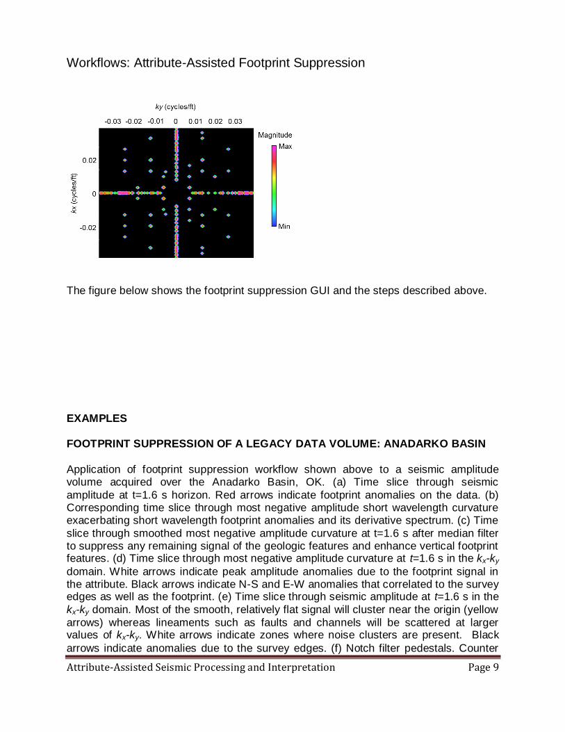
The figure below shows the footprint suppression GUI and the steps described above.

EXAMPLES FOOTPRINT SUPPRESSION OF A LEGACY DATA VOLUME: ANADARKO BASIN

Application of footprint suppression workflow shown above to a seismic amplitude volume acquired over the Anadarko Basin, OK. (a) Time slice through seismic

amplitude at t=1.6 s horizon. Red arrows indicate footprint anomalies on the data. (b) Corresponding time slice through most negative amplitude short wavelength curvature exacerbating short wavelength footprint anomalies and its derivative spectrum. (c) Time

slice through smoothed most negative amplitude curvature at t=1.6 s after median filter to suppress any remaining signal of the geologic features and enhance vertical footprint features. (d) Time slice through most negative amplitude curvature at t=1.6 s in the kx-ky

domain. White arrows indicate peak amplitude anomalies due to the footprint signal in the attribute. Black arrows indicate N-S and E-W anomalies that correlated to the survey edges as well as the footprint. (e) Time slice through seismic amplitude at t=1.6 s in the

kx-ky domain. Most of the smooth, relatively flat signal will cluster near the origin (yellow

arrows) whereas lineaments such as faults and channels will be scattered at larger values of kx-ky. White arrows indicate zones where noise clusters are present. Black

arrows indicate anomalies due to the survey edges. (f) Notch filter pedestals. Counter



intuitively in this step the signal is removed from the data in order to model the noise components. Noise (blue arrows) will then be adaptively subtracted from the data for a noise reduced seismic amplitude volume.



In the figure above: (a) Time slices at t=1.6 s through: original seismic amplitude data, kx-ky filtered seismic amplitude data and noise pattern for the dataset acquired in the

Anadarko Basin, OK. Notice that most of the N-S and E-W lineaments present due to

the footprint in the original data have been removed. Green arrows indicate geologic features that have been enhanced after the filtering. Yellow arrows indicate footprint pattern characterized by the kx-ky filter and removed from the data. (b) Representative

vertical section through the original seismic amplitude data, filtered seismic amplitude data, and noise pattern for the dataset acquired in the Anadarko Basin, OK. Green arrows indicate areas where the signal-to-noise ratio has increased compared to the



original data. Red arrows indicate areas where noise was removed but it is still present. Yellow arrows indicate geologic features removed by the filtering process represented by a kx-ky “noise” component.

FOOTPRINT SUPPRESSION OF A LEGACY DATA VOLUME: DELAWARE BASIN

Application of footprint suppression workflow shown above to a seismic amplitude volume acquired over the Delaware Basin, NM. (a) Time slice through seismic

amplitude at t=0.6 s horizon. Red arrows indicate footprint anomalies on the data. (b) Corresponding time slice through energy ratio similarity exacerbating short wavelength footprint anomalies and its derivative spectrum. (c) Time slice through smoothed energy

ratio similarity at t=0.6 s after median filter to suppress any remaining signal of the geologic features and enhance vertical footprint features. (d) Time slice through energy ratio similarity at t=0.6 s in the kx-ky domain without the application of LoG filter. White

arrows indicate peak amplitude anomalies due to the footprint signal in the attribute. Black arrows indicate N-S and E-W anomalies that correlated to the survey edges as well as footprint. (e) Time slice through energy ratio similarity at t=0.6 s in the kx-ky

domain with the application of LoG filter. The peal amplitude anomalies due to the footprint is more clear that the one in (d). Therefore, we are going to apply (e) in the following workflow. (f) Time slice through seismic magnitude at t=0.6 s in the kx-ky

domain. Most of the smooth, relatively flat signal will cluster near the origin (yellow arrows) whereas lineaments such faults and channels will be scattered at larger values of kx-ky. White arrows indicate zones where noise clusters are present. Black arrows

indicate anomalies due to the survey edges. (g) Time slice through seismic phase at t=0.6 s in the kx-ky domain. (h) Notch filter pedestals. Counter intuitively in this step the

signal is removed from the data in order to model the noise components. Noise (white

arrows) will then be adaptively subtracted from the data for a noise reduced seismic amplitude volume.



In the figure above: (a) Time slices at t=0.6 s through: original seismic amplitude data, kx-ky filtered seismic amplitude data and noise pattern for the dataset acquired in the

Delaware Basin, NM. Notice that most of the N-S and E-W lineaments and localized low

amplitude “spots” present due to the footprint in the original data have been removed. Green arrows indicate geologic features that have been enhanced after the filtering. (b) Representative vertical section through the original seismic amplitude data, filtered

seismic amplitude data and noise pattern for the dataset acquired in the Delaware Basin, NM. Red arrows indicate areas where footprint is strongest. Green arrows indicate areas where the signal-to-noise ratio has increased compared to the original



data. Yellow arrow indicate geologic features removed by the filtering process represented by a kx-ky “noise” component.

REFERENCES Buttkus, B., 2000, Spectral analysis and filter theory in applied geophysics: Springer.

Davogustto, O., and K. J. Marfurt, 2011, Footprint suppression applied to legacy seismic data volumes: to appear in the GCSSEPM 31st Annual Bob. F. Perkins Research Conference.

Drummond, J. M, J. L. A. Budd, and J. W. Ryan, 2000, Adapting to noisy 3D data—Attenuating the acquisition footprint: 70th Annual International Meeting, SEG, Expanded Abstracts, 9–12.

Falconer, S., and K. J. Marfurt, 2006, Attribute-driven footprint suppression: SEG Expanded Abstracts, 27, 2667-2671.

Gülünay, N., 2000, 3D acquisition footprint removal: 62nd Annual International

Conference and Exhibition: EAGE, Extended Abstracts, L0017. Hill, S., M. Shultz, and J. Brewer, 1999, Acquisition footprint and fold of stack plots: The

Leading Edge, 18, 686-695.

workflows: attribute-assisted footprint suppression -...

Documents