working and shirking: equilibrium in public goods … a predetermined age and then shirk thereafter;...
TRANSCRIPT

Dickson and Shepsle 1
Working and Shirking: Equilibrium in Public Goods Games with Overlapping Generations of Players *
Eric S. Dickson Kenneth A. Shepsle
Department of Government Harvard University
Cambridge, MA 02138
Abstract
In overlapping-generations models of public goods provision, in which the contribution
decision is binary and lifetimes are finite, the set of symmetric subgame-perfect equilibria
can be categorized into three types: seniority equilibria in which players contribute (effort)
until a predetermined age and then shirk thereafter; dependency equilibria in which players
initially shirk, then contribute for a set number of periods, then shirk for the remainder of
their lives; and sabbatical equilibria in which players alternately contribute and shirk for
periods of varying length before entering a final stage of shirking. In a world without
discounting we establish conditions for equilibrium and demonstrate that for any dependency
equilibrium there is a seniority equilibrium that Pareto-dominates it ex ante. We proceed to
characterize generational preferences over alternative seniority equilibria. We explore the
aggregation of these preferences by embedding the public goods provision game in a voting
framework and solving for the majority-rule equilibria. In this way we can think of political
processes as providing one natural framework for equilibrium selection in the original
public-goods provision game.
Dickson and Shepsle 2
Working and Shirking: Equilibrium in Public Goods Games
With Overlapping Generations of Players
Eric S. Dickson
Kenneth A. Shepsle
This paper examines the equilibrium norm structure of groups, organizations, even whole
societies, arising out of repeated strategic interaction among members. We use a repeat-play
game theory approach, but we ground our analysis in a set of realistic demographic assumptions –
at least more realistic than is often found in this literature. To keep things simple we focus here
on a group that produces a public good each period in an amount dependent on the contributions
(of effort, time, or some other valuable resource) of group members. As a collective entity the
group’s existence is timeless, but its composition changes. That is, while the group may be
thought of as indefinitely or infinitely lived, the individual members comprising it live finite, non-
coterminous lives. Old members leave the group through death, retirement, electoral defeat, or
term limit, while new members join through birth, enrollment, election, recruitment, or
competitive means. Consequently, at any point in time a cross-section of the group consists of
overlapping generations of members. Some are “rookies” anticipating a long future in the group,
others are in mid-career, while still others are “veterans” with foreshortened time horizons.
In our simple formulation the stage game is one in which each group member decides
whether or not to contribute a unit of (costly) effort to the production of a public good. These
decisions are made simultaneously by group members, the inputs provided are pooled in a public-

Dickson and Shepsle 3
good production process, and an amount of the good is thus produced. All group members enjoy
the public good, with those who have contributed to its production netting out the cost of effort
from their enjoyment level. As we proceed we will provide explicit detail about strategy sets,
payoff function, and information conditions of the stage game. This game is repeated; group
members age, ultimately reaching the end of their tenure in the group; new members arrive. This
is the temporal arrangement.
Substantively, we seek to characterize equilibrium patterns in demographically plausible
settings – those in which individual involvement is temporally bounded, but the institution or
organization or group both precedes and succeeds any particular member in a timeless manner. A
legislature producing public laws and bargaining over distributive benefits is one such instance
(Shepsle and Nalebuff, 1990; McKelvey and Riezman, 1992; Diermeier, 1995; Shepsle, Dickson,
and Van Houweling, 2000), with legislators coming and going but the legislature enjoying a
continuing existence. So, too, is a tribe or village attending to its common defense (Bates and
Shepsle, 1997; Shepsle, 1999) – current tribesmen and -women are both a cross-section of living
generations and part of an intergenerational chain of ancestors and progeny. A hierarchically
organized junta or party replete with unter- and über-officials is a third example (Soskice, Bates,
and Epstein, 1992; Shepsle, 1999).
In the model developed in the next section, conditions are derived that guarantee the
existence of one form of symmetric subgame-perfect equilibrium, called a seniority equilibrium.
The pattern revealed in this equilibrium is one in which a group member makes costly
contributions early in his or her tenure in the group, but this effort ceases at a particular point
when the member effectively is elevated into the ranks of seniors – a tribal elder, a committee
chair, a full professor, a senior bureaucrat, a party leader – and is no longer required to make the
contributions that were necessary earlier. To the proverbial outside observer, a seniority
equilibrium in the cross section looks like an intergenerational transfer scheme – one in which the

Dickson and Shepsle 4
young bear burdens and the old live off the fat of the land. It is what Rangel (1999) refers to as a
backward intergenerational good (BIG), effectively a benefit transmitted “backward” from the
most recent generations to those preceding them.1
Although one purpose of this paper is to present the seniority equilibrium, a second focus
is to show that there are other equilibrium patterns, and that they are logically related to one
another. One of these resembles what social policy makers characterize as dependency –
situations in which neither the very young nor the very old make costly contributions to the
group’s activities. Instead it is the middle-aged who contribute, in effect providing
intergenerational transfers backward to older generations and forward to younger ones. In the
language of Rangel (1999) these are BIGs for the old and FIGs (forward intergenerational goods)
for the young. This is characteristic of social arrangements in advanced industrial societies in
which there is dual intergenerational redistribution – revenue from the taxes on the labor income
of the working middle-aged provides pensions and medical care for retired people and
maintenance and education for dependent children.
Another equilibrium pattern, which we call a sabbatical equilibrium, describes a career in
which there are periods of contribution interrupted by a break (a sabbatical as it were), followed
by subsequent contribution periods (a pattern possibly repeated), ending in a permanent
sabbatical or retirement. Symmetric subgame-perfect equilibria are either of the seniority,
dependency, or sabbatical form.2 Seniority is a special case of dependency, which in turn is a
special case of sabbatical. We are also able to demonstrate for any strict dependency or
sabbatical equilibrium, that there is a seniority equilibrium which Pareto-dominates it ex ante.
These equilibria, as well as the one in which no one ever cooperates (Hobbesian equilibrium), are
displayed in Figure 1, where shaded regions correspond to periods in which an individual
contribution to the public good is made.
**Figure 1 about here**
Dickson and Shepsle 5
The final part of the paper returns to seniority equilibria. We are interested here in political
preferences over working conditions, as it were. Specifically, we explore how intergenerational
majority coalitions support or oppose particular seniority practices.
1 An OLG Model of Public Goods Production3
Preliminaries. Consider a group that meets once per period to decide on the level of a
public good. Individual decisions are made entirely on a voluntary basis where, to keep things
simple, the decision is a binary one – to contribute a unit of effort or not. Time is indexed by t
and is partitioned into periods, i.e., t = 1, 2, …, T,…. During each period the stage game
(described below) is played once by group members “alive” at that time. At the end of each
period payoffs are distributed. The play is then repeated.
At the beginning of each new play of the stage game, a new generation of group members
is “born” and an old generation “dies.” Generation t, Gt, possesses nt members and lives for
exactly T periods. When nt is a constant – assumed here equal to N – exact population
replacement is implied. That is, since the generations that are born and die in each period are the
same size, total population is unchanged.4 There are thus NT players alive in each period. The
oldest generation at time t* is Gt*-T+1 and the youngest is Gt*. The case of T = 3 is portrayed in
Table 1, where there are three generations: young, middle -aged, and old. Each column gives the
composition of the group at time t. A three-element diagonal gives the history of group
membership for a particular generation.
**Table 1 about here**
At each time t, a player chooses one of two actions, “do not contribute” or “contribute.”
That is, the “effort” of i ? G? at time t is eti? ? {0,1}. (In the case where each generation is a
single individual, or can be represented as a unitary actor, i can be suppressed and the discussion

Dickson and Shepsle 6
carried out exclusively in terms of generations as players.) The cost of the “do not contribute”
action is normalized to zero. If an actor contributes, then ? ? 0 is the cost. ? is the same in each
period and across players i.e., no learning effects, aging effects, or other differences among player
types.5
A vector of actions at time t is written et and the output of group activity is a public good,
F(et), where F?(?) ? 0 and F?(?) ? 0. I.e., the group’s production technology is increasing in
group effort, and exhibits (weakly) diminishing returns. (In the development of the model below,
F is assumed linear in the sum of contributed effort.) The stage-game payoff to i ? G? at time t is
F(et) - ? eti?. This is simply the enjoyment from the public good – linear in the amount supplied –
net of contribution. Undiscounted lifetime utility for each player in generation ? is simply the
sum over the stage-game payoffs corresponding to each period {?, ?+1, …, ?+T-1}. (The effects
of discounting are discussed in the extensions section later in the paper.) Each player knows the
demographic structure and production technology of the group, as well as the past history of play.
In sum, a public-good provision game stripped down to its bare essentials is played
repeatedly and indefinitely among finite-lived players. The stage game describes some collective
undertaking in which individuals must determine whether to contribute effort or not. The game is
the same each period, but the composition of the players changes as old players retire and new
players enter. On the basis of individual choices, a collective outcome results with associated
payoffs. Ex post the players know something (perhaps everything) about the choices made by
each of the others in a play of the stage game.

Dickson and Shepsle 7
Throughout we make the following assumptions:
T N
A1. ? ti? = ( ? ? et
i? ) - ? eti?.
?=1 i=1
A2. 1 ? ? ? NT.
In A1 we assume that production is linear in the sum of group effort, and utility for the public
good is linear in production. The payoff to member i of generation ? in period t is this utility net
of the cost of any effort expended. In A2 we restrict our analysis to interesting cost conditions. If
? ? 1 then an individual will always contribute effort since his or her own utility gain from the
increased production exceeds its cost. If, on the other hand, ? ? NT, then even the maximal
amount of public good would not compensate an individual for making a contribution. So we
exclude these uninteresting classes, giving us A2. The cost of effort as specified in A2 gives the
stage game the structure of a prisoners’ dilemma: “do not contribute” is a dominant stage-game
strategy (since ? > 1), but contribution by all members Pareto-dominates non-contribution by all
members (since ? < NT).
As a final preliminary we develop some notation to allow us to characterize all the
equilibrium patterns of repeat-play public goods production games. Let T = {1, 2, …, T} be the
T periods of group membership for an individual. Partition these into two sets, W = {W1, W2, …,
Wk} and S = {S1, S2, …, ST-k}. The first set lists the periods in which the individual contributes to
the group’s public good (“works”), where Wi represents the ith work period. There are k
(endogenously determined) periods of work. The second set lists the periods in which the

Dickson and Shepsle 8
individual does not contribute to the group’s public good (“shirks”), where Si represents the ith
period of shirking. There are T-k periods of non-work. For example, if the practice in the society
described in Table 1 is for its members to work for their first two periods in the group and shirk in
their last period, then T=3 and k=2, with T = {Y, M, O}, W = {Y, M} and S = {O}. That is, W1
= Y and W2 = M, whereas S1 = O.
Motivating Examples. The development thus far is abstract. It is desirable to fix some
examples that the reader may keep in mind. The language of working and shirking suggests the
practices of a labor market, but we believe that modern labor markets are more aptly
characterized by Gesellschaft arrangements like contracts and exogenous enforcement
institutions. Ours, in contrast, is a Gemeinschaft world in which neither official coercion nor
contract necessarily applies. Norms arise as the self-enforcing equilibrium practices of voluntary
behavior. We consider two illustrations of this.
?? Tribal Defense (Bates and Shepsle, 1997). The stage game consists of members of a
tribe providing for its common defense – a public good. The amount of defense is an
increasing function of member effort, but the contribution of effort is costly both because
time has other productive uses and the provision of defense is especially hazardous. Free-
riding is a dominant strategy in this stage game, but some provision of defense Pareto-
dominates the Hobbesian world of no defense. Our analysis focuses on a seniority
equilibrium in which tribesmen contribute effort while young (as “warriors”), and are
relieved of this responsibility when older (as “elders”). Perhaps more appropriate as a
characterization of repeated interaction – in that it comports well with descriptive evidence
– is the idea of a dependency equilibrium in which tribesmen contribute neither when
young nor when old. In raw youth they may not be capable of providing effort toward the
public good, instead serving more modest family objectives (minding animals, doing
household chores). In their older years they enjoy the privileges of land ownership, cattle,

Dickson and Shepsle 9
and wives, both as reward for earlier service and in recognition of the fact that their ability
to provide for defense has atrophied. In between they provide effort toward defense of the
tribal realm. In either the seniority or dependency equilibrium pattern, the question arises
of how much defense can be provided – indeed, can any positive amount be sustained? –
and, as a comparative statics matter, how this provision varies with changes in the cost of
effort (? ), life expectancy (T), size of generational cohort (N), and production technology
(F).
?? Legislative parties. As a second illustration, consider a legislative party consisting of
politicians who share common policy objectives but are at different career stages.
Achievement of their preferred policies requires effort. But the contribution of such effort
for the common objective means that the politician must forego valuable private activities
– campaigning, pork barreling, constituency service, preparation for a post-legislative
career. That is, the party public good comes at a private cost. A seniority equilibrium in
this case would consist of senior members claiming credit for party successes and
otherwise using public accomplishment for private purposes without doing any of the
“donkey work” that is required of the more junior party members. As the latter become
more veteran, they will no longer be required to make private sacrifices since these will be
shifted onto still newer party members. As a variation on this equilibrium practice, it may
be necessary for the most junior members to devote effort to “making their districts safe,”
and because of this be granted a grace period during which they are not expected to
contribute much in the trenches to party public goods. This variation serves as another
example of a dependency equilibrium.
Dickson and Shepsle 10
2 Seniority Equilibrium
Generally speaking, the idea of a seniority practice is that a young group member works
hard, bears burdens, makes sacrifices, and foregoes opportunities, expecting other young
members to do the same. In exchange for this the member has burdens lightened, sacrifices
diminished, and opportunities enhanced in his or her later years in the group. This arrangement
lends itself to two interpretations, one longitudinal and the other cross-sectional. From a
dynamic, individual perspective, it may be construed as deferred gratification, investment in
career, or a “retirement” bonus for service in the organization. This perspective interprets
seniority as early pain for later gain – i.e., early-to-late intertemporal redistribution over an
individual’s life in the group. From the static, collective perspective, on the other hand, it is an
instance of intergenerational redistribution from the currently young to the currently old. It is, in
effect, a pay-as-you-go pension scheme.
For k ? {0,1,…,T}, a k-seniority practice is a partition of T into two sets, W and S. The
first comprises k periods of work (contribution of effort toward the public good) and the second
T-k periods of non-work (non-contribution), such that Wj = j (j ? k). Thus, W1 = 1, W2 = 2, …,
Wk = k, and S1 = k+1, S2 = k+2, …, ST-k = T. The first work period is the member’s first period
in the group, the kth work period is the member’s kth period in the group, and the first “shirk”
period is not until the member’s (k+1)st period in the group. Importantly, the two sets in the
partition are unbroken. As we shall see this distinguishes seniority arrangements from other
equilibrium practices. A k-seniority practice is a seniority equilibrium if and only if it is subgame
perfect in the public goods game. A seniority practice is an equilibrium, that is, if at no age does
a member have an incentive to defect from the practice.
Two preliminaries follow immediately from this definition. First, it is easy to see that the
degenerate T-seniority practice (k=T) is not a seniority equilibrium. The T-seniority practice
Dickson and Shepsle 11
requires work in every period, and yet no one will contribute in his or her last period since this
effectively requires playing a dominated strategy in a one-shot PD stage game. This means that,
from a normative perspective, even though it is socially desirable for group members to
contribute every period – from assumption A2 – this will not constitute equilibrium behavior; at
most we can have a (T-1)-seniority equilibrium. Second, the degenerate 0-seniority practice
(k=0) is an equilibrium. This seniority practice is the Hobbesian equilibrium of the state of nature
in which no one contributes in any period, and no public good is produced at all. It is, of course,
well known that the repeated application of this stage-game equilibrium is an equilibrium of the
repeat-play game, and that is what the 0-seniority practice is.
For 0 ? k ? T, a k-seniority practice is an equilibrium if and only if, for every group
member at every age, the continuation value of playing in accord with the practice exceeds the
continuation value of deviating from it. According to the equilibrium, N members from each of
exactly k generations will contribute effort each period, so every member enjoys Nk units of the
public good per period; a contributor, however, must net out the contribution cost of ? . For a
member with kr remaining contribution periods, 0 ? kr ? k, the continuation value of remaining on
the equilibrium path is6:
U(kr) = kr (Nk - ? ) + (T-k)(Nk).
The continuation value of deviating depends, of course, on what happens to someone who
deviates. The grim-trigger punishment strategy is one in which any deviation is followed by
everyone in the group choosing permanent non-contribution.7 Thus, a deviant – someone who
does not contribute when he or she should – receives Nk-1 in the period of deviation, and zero
thereafter. It follows, then, that a k-seniority practice is an equilibrium only if U(kr) ? Nk-1 for
every kr.

Dickson and Shepsle 12
Two possibilities arise depending upon the exogenous cost, ? . If ? is small enough, so that
all individuals receive positive payoffs each period, even in those periods in which they
contribute effort to the public good, then it may be possible to sustain a k-seniority practice as an
equilibrium. This circumstance is characterized in Proposition 1 (and was initially proved by
Cremer, 1986). On the other hand, if ? is large, then the seniority practice will require
contributors to bear early net losses in equilibrium. Nonetheless, there are circumstances in
which certain k-seniority practices may be sustained as equilibria. This case is examined in
Proposition 2.
Several preliminaries are presented first. Consider a general k-seniority practice.
Claim 1. If Nk ? ? , then a member who would not defect in period Wk – the last
period of contribution – will not defect earlier.
In a trigger-strategy punishment regime, the continuation value from defection is Nk-
1, and this holds whenever one defects during the contribution phase, W. Let the
continuation value along the equilibrium path of a member with kr remaining
contribution periods be U(kr), where 0 ? kr ? k. Under the condition of this Claim,
U(kr-1) ? U(kr) – the continuation value of complying with the putative equilibrium
is decreasing in time. This is because as each period passes, the continuation value
of complying declines by Nk - ? , a positive payoff by the premise of this Claim. So
if U(1) ? Nk-1, then U(kr) satisfies the inequality for kr ? 1, i.e., if one does not
defect in the last contribution period, he or she will not defect in any earlier period
either.
Claim 2. If Nk ? ? , then a member who does not defect in period W1 – the first
period of contribution – will not defect later.

Dickson and Shepsle 13
Here the logic is the same, but the inequality runs the other way – U(kr) ? U(kr-1).
So, if U(k) ? Nk-1, then U(kr) satisfies this inequality for kr ? k.
These preliminary claims provide us with a method for establishing the conditions under
which a seniority practice is an equilibrium. If Nk ? ? , then Claim 1 provides the inequality that
must be satisfied for a k-seniority practice to be an equilibrium. If, on the other hand, Nk ? ? ,
then the inequality given in Claim 2 is germane. We establish conditions for seniority equilibria
in the next two propositions.
Proposition 1. Consider the game with period t payoff function given by A1,
cost of effort given by A2, and k ? {0,1,…,T-1}. If Nk-? ? 0, then the k-
seniority practice in which every member of each generation contributes for his
or her first k periods and does not contribute thereafter (unless someone has
deviated from this in an earlier period, in which case perpetual non-cooperation
is chosen) is a subgame perfect equilibrium.
To prove this result we appeal to Claim 1 and examine the inequality that must hold
in period Wk: (Nk-? ) + Nk(T-k) > Nk-1, or, with some algebra, (T-k)k > (? -1)/N.
But from the premise of Proposition 1, k ? {0,1,…,T-1}, and this implies that (T-k)k
> (1)k. And Nk-? ? 0 implies that k > ? /N and, a fortiori, k > (? -1)/N. Stringing
these inequalities together we see that the inequality of Claim 1 is satisfied. There
will be no defection from this k-seniority practice, and Proposition 1 is proved.
The notion here is that for ? small enough it will be possible to sustain a particular k-
seniority practice in a relatively painless way – namely one in which even contributors are net
beneficiaries each period. Indeed, so long as Nk = ? it will be possible to sustain any k-seniority
practice as an equilibrium for k < T.

Dickson and Shepsle 14
When net burdens must be borne during contribution periods, however, then additional
conditions must be satisfied, as demonstrated in the next proposition.
Proposition 2. Consider the game with period t payoff function given by A1,
cost of effort given by A2, and k ? {0,1,…,T-1}. If Nk-? ? 0 and if (T-1) k ? (k ?
- 1)/N, then the k-seniority practice in which every member of each generation
contributes for his or her first k periods and does not contribute thereafter
(unless someone has deviated from this in an earlier period, in which case
perpetual non-cooperation is chosen) is a subgame perfect equilibrium.
The proof of this result requires an appeal to Claim 2 in which non-defection in the
first contribution period is necessary. This means that U(k) > Nk-1 must hold. That
is, k(Nk-? ) + (T-k)Nk > Nk-1, which simplifies to the required inequality. (Clearly,
if T-1 ? (? -1)/N, then at least one period of contribution toward the public good can
be sustained as an equilibrium).
For high-cost public goods production processes, in which group members bear net losses
during periods of contribution, it may still be possible for an equilibrium k-seniority practice to
exist. This is the message of Proposition 2.
It may seem remarkable that we are able to derive non-Hobbesian equilibria at all. Our
agents, after all, are group members for finite periods of time. In many analyses with finite-lived
agents, there are end-game problems and unraveling that destroy any but the Hobbesian
equilibrium. It is the overlapping-generations structure, however, that overcomes the problem of
unraveling that often haunts finite repeat-play PD games.8 There is a price – namely, some
unraveling such that only second-best equilibria are possible. In this analysis we have also
learned that the truncated 0-seniority practice (the Hobbesian outcome) is an equilibrium, but not
a very interesting one either as a seniority practice or as an equilibrium. The T-seniority practice,

Dickson and Shepsle 15
on the other hand, cannot even be an equilibrium. Finally, we see that the “length” of the
contribution period is driven by the cost parameter, ? , but that non-trivial cooperation can take
place even in groups in which the cost of effort is high.
Propositions 1 and 2 provide an algorithm for determining whether or not a given seniority
practice is an equilibrium. However, they do not establish the existence of equilibria, and they do
not provide a mapping from the parameters of the model onto the set of seniority practices, if any,
which are in equilibrium. These are established in the following:
Proposition 3. Consider the game with period t payoff function given by A1, cost of
effort given by A2, and k ? {0,1,…,T-1}. Then
all k ? T-1 are equilibria if ? ?? (1, N(T-1)+1/(T-1)]
all k ? 1/(? -N(T-1)) are equilibria if ? ?? (N(T-1)+1/(T-1), N(T-1)+1]
k = 0 is the only equilibrium if ? ?? (N(T-1)+1, NT).
This is displayed in Figure 2. We see that the range of equilibrium practices is weakly increasing
in T, weakly increasing in N, and weakly decreasing in ? ???Further, if it is the case that some
practice k’ is a seniority equilibrium, then all practices k<k’ are also seniority equilibria. For a
given set of parameters N, T, and ? , we will refer to the largest equilibrium value of k as kmax.
**Figure 2 about here**
These results, we believe, are suggestive of the stylized regularities of many group settings
where seniors are the beneficiaries of group life, but only after first paying their dues as juniors.
Thus, referring back to our first running example, tribal defense is provided from the warrior-like
effort of younger members of the tribe, while privileges are enjoyed by elder members. And,
from the legislative example, common party policy positions are developed and advanced, with
all members “claiming credit” but junior members expected to do most of the work in the

Dickson and Shepsle 16
trenches. This pattern of seniority, however, does not exhaust the possibilities for equilibrium.
We explore alternatives in the next two sections.
3 Dependency Equilibrium
Informally, the idea of a dependency practice is that in some groups neither the very young
nor the very old contribute to the provision of public goods. Thus, there are two discontinuities in
the career of a group member, often identified by symbolic “rites of passage.” One is the move
out of dependency and into active group life (“Today I am a man.”). The other is the move out of
active group life and into a phase of privileged inactivity (symbolized by a pension and a pocket
watch).9
Formally, we define (in a manner parallel to our earlier definition) a k-dependency practice
as a partition of T into three sets such that Wj = j + b for fixed b ? {0, 1, 2, …, T-k}. This simply
says that there is a single continuum of periods during which an individual’s contributions to the
public good are made, and that this continuum may be “interior” to his or her tenure in the group;
on each side of the contribution continuum is a shirking continuum. The first work period, W1,
occurs in the (1+b)th period of a person’s life in the group, and this continues for a total of k
periods. A k-dependency practice is a dependency equilibrium if and only if it is subgame perfect
in the public goods game. Notice that b = 0 reduces a k-dependency practice to a k-seniority
practice. Hence, seniority is a special case of dependency. We refer to a dependency practice
(equilibrium, resp.) for which b ? 0 as a strict dependency practice (equilibrium, resp.). Notice,
also, that b = T-k is a k-dependency practice with no terminal phase of privilege – the k periods
of contribution are back-ended. No such k-dependency practice is an equilibrium, i.e., a non-
trivial terminal period of privilege is a necessary condition for equilibrium.
To simplify the analysis we rewrite notation so that an individual’s experience in the group
is given by dependency in periods 1 to D, contributions of effort from period D+1 until period P,

Dickson and Shepsle 17
and privilege from period P+1 through period T. In neither the dependency nor the privilege
phase does the member make contributions:
?? Dependency: D periods
?? Contribution: P-D periods
?? Privilege: T-P periods.
We now determine whether this arrangement (a (P-D)-dependency practice with b = D, in the
earlier notation) is a dependency equilibrium. To accomplish this we must show that no member
has an incentive to behave in other than the prescribed way. Note that the payoff to an individual
is (P-D)N in each period of the dependency and privilege phases, and (P-D)N-? during each
contribution period. It should be obvious that an individual will never defect in either a
dependency or privilege period. (In each of these periods an individual enjoys (P-D)N units of
the public good at no cost, and such enjoyment in no way commits the individual to a particular
course of action during the contribution phase.)
Consider first a group member in his or her last period of contribution. He or she will earn
(P-D)N-? in this period, followed by (T-P) periods of (P-D)N, for a continuation value of (T-
P+1)(P-D)N-? . The continuation value of defecting is (P-D)N-1. The difference between these
two terms is non-negative when
(T-P)(P-D)N ? ? -1. (1)
Since we have effectively set k = P-D, this inequality is the relevant condition that assures no
member will defect whenever (P-D)N ? ? (the premise of Claim 1 above). But notice that the
premise of Claim 1 implies that (T-P)(P-D)N ? ? so long as T-P is greater than one. That is, (1)
will hold when the premise of Claim 1 holds so long as there is a non-trivial period of privilege.
This establishes

Dickson and Shepsle 18
Proposition 4. Consider the game with period t payoff function given by A1,
cost of effort given by A2, and (P-D)-dependency practice with b=D. If (P-D)N-
? ? 0, and if the length of the period of privilege is such that P ? T-1, i.e., the
privilege phase commences before the next-to-last period, then the dependency
practice in which each member does not contribute for his or her first D
periods, contributes for the next P, and then does not contribute thereafter
(unless someone has deviated from this in an earlier period, in which case
perpetual non-cooperation is chosen) is a subgame -perfect equilibrium.
In effect, Proposition 4 says that if the (interior) continuum of group contribution in the life of a
member is sufficiently long relative to the cost of effort, then an equilibrium exists which
accommodates both early dependency, end-game privilege, and a positive level of the public
good. The next result indicates that positive public good production is possible even when the
productive period of a member’s life in the group is relatively short.
Consider now a group member in his or her first period of contribution – the member’s
(D+1)st period in the group. The continuation value for this member, if he or she remains on the
equilibrium path, entails (P-D)N units of the public good per period for the remainder of time in
the group – T-D periods – but P-D periods in which a contribution is required at a cost of ? per
period. Putting these together we have a continuation value of (T-D)(P-D)N - (P-D)? . Defection
at this time yields a continuation value of (P-D)N-1. Defection will not take place in this first
contribution period, therefore, if
(T-D-1)(P-D)N ? (P-D)? -1. (2)
From Claim 2, if (P-D)N ? ? , then (2) provides the condition for a dependency equilibrium. This
establishes
Dickson and Shepsle 19
Proposition 5. Consider the game with period t payoff function given by A1,
cost of effort given by A2, and (P-D)-dependency practice with b=D. If (P-D)N-
? ? 0, and if (2) holds, then the dependency practice in which each member does
not contribute for his or her first D periods, contributes for the next P, and then
does not contribute thereafter (unless someone has deviated from this in an
earlier period, in which case perpetual non-cooperation is chosen) is a subgame -
perfect equilibrium.
A little manipulation of the two requirements in Proposition 5 yields a conclusion very similar to
that of Proposition 4 – that a dependency practice with, in this case, a high cost-of-production
technology is an equilibrium so long as there is a non-trivial period of privilege (P ? T-1).10
We have noted that dependency often arises endogenously as a consequence of production
technology and cost.11 In Propositions 4 and 5, however, we have taken D as exogenous.
Nevertheless, we can ask what dependency parameters a group would choose if it were free to do
so – noting that the choice of D=0 is to transform dependency into seniority.
To begin we may ask: what values of D and P – for a given N, T, and ? – maximize
individual lifetime utility? In effect, this is a behind-the-veil question in which we seek to
determine what parameter values are best for an individual ex ante. For particular D and P, ex
ante lifetime utility from complying with these values entails D periods of [(P-D)N], followed by
P-D periods of [(P-D)N-? ], and then followed by another T-P periods of [(P-D)N]. Adding these
up yields (P-D)(NT-? ). The second term is fixed and positive (by A2). Thus, ex ante lifetime
utility is maximized when P-D is maximized, i.e., D=0 and P=T. But this cannot be an
equilibrium, since an individual will not contribute in his or her last period. Can we instead make
a useful generalization about the relative ex ante welfare implications of different types of
second-best equilibria? As an example, in Appendix B we demonstrate that

Dickson and Shepsle 20
Proposition 6. For any strict dependency equilibrium, there is a seniority equilibrium
that Pareto dominates it ex ante.
All other things equal, seniority practices are superior to dependency practices among second-
best forms of social organization – superior in the sense that dependency sacrifices social surplus;
second-best in the sense that, even if it is desirable for people to contribute to the production of
the public good every period, it is not possible to induce this as an equilibrium response.
4 Sabbatical Equilibrium
A distinguishing feature of both seniority and dependency practices is, to put it
colloquially, that life is divided into working and shirking. More accurately, life is divided into
phases, or epochs, or continua – some requiring working and others allowing shirking. In the
case of a seniority practice, life is partitioned into an early continuum (possibly of length zero –
the Hobbesian equilibrium) in which contribution to the group’s activities is required, and a later
continuum during which contribution is not expected – k periods of work followed by T-k periods
of non-work. In the case of a dependency practice, a continuum of non-contribution (possibly of
length zero) precedes the seniority pattern – D periods of non-contribution, followed by P-D
periods of contribution, and then T-P more periods of non-contribution. We have seen that for
either of these practices to be an equilibrium, it is necessary that there be a non-trivial phase of
non-contribution at the end of a person’s group tenure.
A third pattern, which we call a sabbatical practice, is characterized by nonconsecutive
work. There may be an initial period of non-work – as in a dependency practice. There
necessarily is a non-trivial non-work period at the end of a member’s term in the group – as in a
seniority practice. However, the set of contribution periods need not constitute a continuum, but
rather may be interrupted by periods of sabbatical (mid-career non-work). As the reader surely
sees, a sabbatical practice is a generalization of dependency which, in turn, generalizes seniority.

Dickson and Shepsle 21
Formally, let b be the number of periods before the first contribution period, i.e., W1 = 1+b.
A k-sabbatical practice is one in which, for k the number of contribution periods in a member’s
term in the group, the final contribution period is not 1+b+k. i.e., Wk ? 1+b+k. A sabbatical
practice is not a k-period contribution continuum beginning in period 1+b and concluding in
period 1+b+k. Contribution periods are interrupted by one or more sabbaticals of one or more
periods in which no contribution is made. A sabbatical practice is a sabbatical equilibrium if and
only if it is subgame perfect in the public good production game.
While we do not develop this category of equilibrium here, we note some new features that
arise. A complication associated with sabbatical equilibria that we haven’t encountered in the
other situations is informational. The rules governing sabbatical leaves must be very clear to the
members of the group. Whenever a person is not working, it must be evident to all that he or she
is entitled to be “on leave.” In a seniority practice the commencement of the privilege phase is
often marked by a ritualistic rite of passage. Likewise, the transition from shirk to work in a
dependency practice is also often marked by formal ritual. In each case there is a career
discontinuity that is common knowledge. Sabbaticals are trickier, requiring better information,
careful monitoring, and sometimes the capacity to verify in an audit.12
5 Time-Dependent Preferences over Equilibria
For many fixed values of the demographic and technological parameters, a large number of
equilibrium arrangements will be feasible. In Section 3, we derived a few results concerning the
relative ranking of these equilibria with respect to the ex ante lifetime utility they provide. In
particular, we demonstrated in Proposition 6 that each strict dependency equilibrium is Pareto-
dominated ex ante by at least one seniority equilibrium, and that the maximal seniority practice
(D=0, P=T-1) provides the greatest ex ante lifetime utility when this practice is an equilibrium.
These results provide intuition as to which practice might be selected by a benevolent social

Dickson and Shepsle 22
planner or behind a veil of ignorance, a state in which individuals lack information about their
particular private interests.
However, it is a stubborn fact of politics that real people tend to make decisions with their
personal interests very much in mind. A major contribution of formal theory to political science
has been its logical explication of the frequent conflict between individual interests and socially
optimal decision making. Even “second-best” equilibrium social practices may not be attainable
when selection is embedded in a political process. Whether this is so depends upon the particular
details of this decision-making process.13
In this section, we delve more deeply into these issues by considering individual
preferences over social practices and the ways in which these preferences change over time. It is
a central tenet of rational choice theory that individuals honor neither sunk costs nor sunk benefits
in deciding on future courses of action. Because of this, the rewards and obligations of the past,
once relevant to the individual’s optimization problem, no longer matter, and time inconsistencies
in actor preferences can be expected to arise as time unfolds in our overlapping-generations
world. Of course, we have already dealt with this implicitly when determining which social
practices are in equilibrium; we now turn our attention to the separate question of which ones an
individual can be expected to prefer as a function of his or her age.
For simplicity, we fix the demographic and technological parameters N, T, and ? , and
restrict our attention to k-seniority practices that are in equilibrium. How do preference orderings
over the equilibria in this set change as individuals grow older?
We begin our formal analysis by calculating the future value of each seniority equilibrium
for an individual in period t of play. By comparing the future value for two distinct equilibria, k
and k’, we can determine an age-t individual’s ranking over these alternative social arrangements.
The future value of a particular equilibrium for an individual is simply the aggregate quantity of
public goods produced per period times the number of periods he has remaining, minus the cost

Dickson and Shepsle 23
of effort per working period times the number of working periods he has remaining. An
individual at the beginning of period t will live for a further T-t+1 periods, while he will work for
a further k-t+1 periods if t ? k and not at all if t ? k. This implies that
Nk(T-t+1) - ? (k-t+1) if k ? t
FV(k,t) = (3)
Nk(T-t+1) if k < t.
A few properties of the preference orderings implicit in this future value function are contained in
the following proposition.
Proposition 7. Consider the set of equilibrium seniority practices, indexed by k.
?? The preference orderings of the youngest and the oldest generations are
always the same, and are identical to the ordering obtained by ranking the
alternatives according to their ex ante values.
?? For every generation, preferences over equilibrium seniority practices are
single -peaked in k.
The proposition is proved in Appendix C.
The first part of the proposition can be understood in the following way. Individuals from
the youngest generation are at the beginning of play, and hence their future value function is
identical to the ex ante value function. Their preferences are monotonic in equilibrium levels of
k. Consider now individuals in the last period of play. As we previously stated, such individuals
can never be expected to contribute in equilibrium, but they will wish for the level of public
goods production to be as large as possible to maximize their own consumption. As such, they
will naturally prefer equilibria with larger values of k to those with smaller values. Thus we see
that, in a world without discounting, the youngest and the oldest will always agree in our model,
and there is no distinction between their preferences and those of a benevolent social planner.
Dickson and Shepsle 24
Matters are rather more complicated for members of intermedia te generations. For
example, consider the incentives of an individual in his eighth period of play when life span is
eleven periods, i.e., T=11. On the one hand, the larger the value of k , the more public goods he
will be able to enjoy, both during work and in retirement. On the other hand, there is now at least
one potential reason for him to prefer a k=7 regime to a k=8 regime: he could spend the present
period shirking in the first equilibrium but not in the second. Which value of k he prefers will
depend upon the relative cost of working. If ? is small compared to the public goods benefit that
would be produced by having everyone else in his generational cohort work, then he will prefer a
social arrangement in which he himself works during the eighth period. If however ? is not so
small, we can expect to observe preference reversals during the aging process. Whether or not an
individual works in the eighth period of play is water under the bridge when that individual is in
his eleventh period of play, but not when he is in his eighth.
An intuitive feel for these concepts can be obtained through an examination of Figures 3
through 5. Each figure contains the future value curves corresponding to the seniority equilibria
that exist for one particular set of parameter values. The graphs display preference curves for
individuals from different generations. T and N are fixed and ? ?is allowed to vary from figure to
figure. Note that all of the curves are single -peaked and that the curves corresponding to the
youngest and oldest generations (represented by thick lines) are monotone increasing.
**Figures 3, 4, and 5 about here**
In our discussion of ex ante lifetime utilities, we noted that maximal k-seniority practices
have a particular focal property when they are in equilibrium. Now, however, the situation is
more complicated, as we have age-dependent preferences and cannot count on the unanimity that
would exist behind the veil of ignorance. One obvious means of aggregating these preferences is
through simple one-man-one-vote majority rule (in the simple demographic case of fixed
generation size that we consider here, this is effectively “one-generation-one-vote”). Of course, it

Dickson and Shepsle 25
is typical of real human societies that an asymmetry of power and influence exists among
generations, as tribal elders and senior congressmen illustrate. For the moment, however, we will
assume that each individual has equal influence in selecting the social arrangement. Given the
preferences of members of our model society, as established in the previous proposition, one k-
regime typically constitutes a majority-rule equilibrium – the median most-preferred k.
The following proposition summarizes this result.
Proposition 8. There exists a majority-rule equilibrium in intergenerational voting
over seniority equilibria, and the social preference order over all k-seniority equilibria
under simple majority rule is transitive.
The proof of the proposition is in Appendix D.
A Condorcet winner exists in each of the Figures 3-5. In Figures 3 and 4, it is the socially
second-best optimum, k=10, the result that would emerge “behind the veil.”14 In Figure 5,
however, it is k=8. This establishes that a majority-rule equilibrium need not be the maximal k-
seniority equilibrium that would have been chosen behind the veil.
In fact, we can derive a mapping from parameter values to Condorcet winner directly and,
more interestingly, carry out some simple comparative statics. This we do next, relegating details
and the proof to Appendix E. Let floor(?) be a function rounding its argument down to the
nearest integer.

Dickson and Shepsle 26
Proposition 9. Let kCW be the Condorcet-winning number of work periods. If T is
odd and if T? 7, then
T-1 if ? ?? (1, N(T+5)/2)
floor(T+1-? /N)+(T-1)/2 if ? ?? [N(T+5)/2, N(T-1)+1/(T-1)]
kcw = (T+1)/2 if ? ?? (N(T-1)+1/(T-1), N(T-1)+2/(T+3)]
floor(1/(? -N(T-1))) if ? ?? (N(T-1)+2/(T+3), N(T-1)+1]
0 if ? ?? (N(T-1)+1, NT).
(Analogous results for T=3 and T=5 can be found in Appendix E.) kCW is a weakly
increasing function of T – as individual life span increases, the Condorcet-winning
number of working periods either increases or remains the same. kCW is also weakly
increasing in N – as the cohort size grows, the majority-preferred number either
grows or stays fixed. Finally, kCW is a weakly decreasing function of ? – as it
becomes costlier to contribute, the amount of work in a majority-rule voting
equilibrium decreases over some intervals and remains the same over others.
As an illustration, Figure 6 displays kcw as a function of ? for a particular value of the
parameter pair (N,T).
**Figure 6 about here**
It is commonplace in repeated games for a multiplicity of equilibria to exist, and in this
regard overlapping-generations games are no different. Typically, as we have shown, multiple
equilibria exist even when one restricts attention to seniority practices. Proposition 8 suggests an
equilibrium refinement for overlapping generations games – namely, examining the robustness of
equilibria to majority rule. In certain contexts, especially those in which the selected social
practice is endogenously chosen by some political process, it may make sense to argue that a

Dickson and Shepsle 27
Condorcet-winning practice is more likely to be observed over the long-run, since it will always
be in the interests of a majority to renegotiate any equilibrium that is not a Condorcet winner.
The plausibility of such evolutionary appeals will of course differ depending on the particular
application of interest.
6 Extensions
In the present paper we have characterized equilibrium arrangements for the organization
of work, broadly construed. In effect we provide conditions under which individuals engaged in
the production of a public good, and organized into overlapping generations of members, are able
to arrange a pattern of cooperation that enables them to escape the Hobbesian equilibrium of zero
supply. With finite-lived agents it will not be possible to produce public goods optimally (as
conventionally defined), since it is not possible to induce a last-period willingness to contribute.
But, so long as the individual cost of contribution (? ) is sufficiently low relative to other social
parameters (generation size, N, and life span, T), some positive level of group production is
sustainable as an equilibrium. The equilibria sort themselves into three types – strict seniority,
strict dependency, and sabbatical.
Needless to say our results have not been produced under particularly general conditions,
though some version of them is likely to survive relaxation of various assumptions. Of the many
possible extensions along these lines, there are several that we believe are of special interest.
?? Variable cost of effort. The parameter ? is a constant in the results we present – across
individuals of the same generation and throughout the life of any individual. This
abstracts away not only differences in natural endowments (the differences within a
generational cohort that can be taken as exogenous), but also the variations in human
capital associated with aging and experience. Letting t represent a continuous measure of
length of elapsed tenure in the group, a learning effect may be represented by ? ?(t)

Dickson and Shepsle 28
<while an aging effect would have ? ?(t) > 0. In a mix of these, as seems intuitively
plausible in many circumstances, ? (t) declines until “mid-life” and then increases
thereafter.
A tribesman grows increasingly adept at providing warrior services until his physical
attributes begin to atrophy. At the same time, experientially based human capital permits
acquired guile and intelligence to reduce the cost of effort. Early in life, then, the trend
on ? is downward but, unless the learning effect dominates late in life, eventually ?
begins to increase as declining physical skills become controlling. These effects provide
endogenous pressures for social norms of “dependency” and “privilege.” A high ? when
a tribesman is very young would dispose a tribe to allow the talents of youngsters to
remain with private family activities for which they are more suited, while a high ? when
the tribesman is old would dictate relieving him of physically demanding effort (though
perhaps not from governance responsibilities for which the stock of guile and intelligence
is still appropriate). The career of a legislator, on the other hand, is more likely to be
affected through most of his or her career by the learning effect, with the aging effect
coming into play only at a very advanced age. Legislative warriors, so to speak, can
remain active for a considerable part of their legislative career, improving with age for
most of that period (see Shepsle and Nalebuff, 1990).
A variable ? is decidedly more realistic, and raises a host of quite interesting issues. As
mentioned, it would permit a more incisive analysis of dependency phenomena.15 It
would also allow for intra-generational differences to emerge, thereby compelling
attention to personal characteristics other than age in accounting for manifest differences
in participation in the life of a group, even among those from the same generational
cohort. Of course, these raise complexities exceeding the scope of the present, more
modest undertaking.
Dickson and Shepsle 29
?? Discounting. Discounting must accommodate both impatience and uncertainty.
Discounting for impatience reflects the fact that most individuals assess the utility of an
outcome in terms of the imminence of the associated benefits and costs. Discounting for
uncertainty reflects the fact that individuals take on board the prospect that there is some
probability they will not be in a position to enjoy benefits or bear burdens in some future
period. The first effect, perhaps the result of physiological hard-wiring, is a reasonable
assumption in most settings. As the future is discounted more heavily, any deal involving
promises of future benefits in exchange for bearing present burdens – as in our seniority
equilibrium – will be harder to sustain as an equilibrium. To satisfy incentive
compatibility constraints, it will be necessary either for less delay, bigger benefits, or
smaller costs. As such, one might expect dependency and sabbatical equilibria to play an
increasingly prominent role as the future is discounted more. In effect, impatience-
induced preferences provide another basis for endogenizing dependency periods and
sabbatical leaves as mechanisms for bringing net benefits forward.
The second basis for discounting – uncertainty – is technically more complicated, for it
forces a revision of the assumption of a fixed term of membership, T. Not only will an
individual be uncertain that he or she will be around to consume future benefits, but this
uncertainty will also extend to beliefs about the continued presence of, and contributions
by, other group members. This form of discounting will have a deleterious effect on
intertemporal cooperation in groups.
?? Production technology. An obviously restrictive feature of our analytical exercise is the
assumption that F(e t) is linear in the sum of effort contributions. This would constitute a
natural opportunity for extension, though it is not clear that any particular functional form
would cover a very wide range of phenomena. The production of military defense may,
over some ranges, be convex in effort, for example. Legislative production, on the other

Dickson and Shepsle 30
hand, may exhibit diminishing returns (indeed, possibly decreasing returns above some
level).
?? Asymmetric equilibrium. The seniority, dependency, and sabbatical equilibria we
identify are symmetric in the sense that individuals are treated identically, and like
individuals are assigned like equilibrium behaviors. Every individual is identical in the
sense that he or she lives exactly T periods, and has the same utility function, strategy set,
cost of effort, strategic opportunities, and information. The only feature distinguishing
individuals in any play of the game is age. By “symmetric” we mean that the equilibria
we identify stipulate equilibrium behavior in which age, and only age, determines who
contributes and who does not to the group’s public good. It occurs to us, however, as it
must to any student of human history and social behavior more generally, that various
groups and societies often organize themselves on the basis of characteristics other than
age. It would be of great interest to extend the kinds of arguments offered here to a world
in which there were, for example, elites and plebes. A seniority equilibrium that also
acknowledged social stratification would be a (ke, kp)-seniority practice in which elites
worked for ke periods, followed by T-ke periods of shirking, whereas plebes worked for
kp periods (presumably greater than ke).16
?? Age-dependent preferences. Finally, we note that it is of interest to extend the idea of
age-dependent preferences over group norms, and of voting in each period to sustain or
change some group norm, beyond seniority to the other equilibrium notions –
dependency and sabbatical.
7 Conclusion
We have provided a simple model establishing conditions under which a group of
constantly changing composition sustains collective cooperation over time and thereby provides

Dickson and Shepsle 31
itself with some level of a public good. We show that such practices may be partitioned into
seniority, dependency, and sabbatical equilibrium types, reflecting the various ways in which
contribution-of-effort requirements can be programmed. Of the many seniority practices that are
sustainable in equilibrium, we establish that collective choice by majority-rule voting refines
these, yielding in the case of odd-numbered groups a unique equilibrium amount of cooperation.
This follows from the median voter theorem and the single -peakedness of preferences over the
number of periods of cooperation – preferences that change in a regular and predictable fashion
with a member’s tenure in the group. The single -peakedness of age-dependent preferences – and
the concomitant majority-rule equilibrium this supports – is one of the more interesting
discoveries reported here. It allows us to characterize equilibrium even in circumstances in which
member preferences are not fixed, ex ante, as is the customary assumption in social choice-
theoretic analyses.
It is tempting to conclude by extending even further the list of extensions given in the
previous section. But we will only do so in a highly abbreviated fashion by offering some final
remarks concerning enforcement. Our model is one of circumstances in which a contractual
solution is unavailable, due to an absence of external sources of enforcement. The grim-trigger
form of self-enforcement on which our results are founded, however, seems implausible in two
respects. First, there is the problem of renegotiation, on which we are silent. Second, and related,
there is the idea that targeted punishment, especially in a world of full information, is both more
credible and more easily implemented than the grim-trigger alternative. Certainly the
anthropological literature is replete with instances of violator-specific mechanisms for dealing
with failures to behave in accord with group norms – of shunning, ostracizing, and banishing
shirkers rather than totally disbanding the group. The warrior who avoids his responsibilities is
sent into the wilderness to fend for himself. The party politician who violates the party work
ethic – behaving as a “show horse” when he or she should have been a “work horse,” for

Dickson and Shepsle 32
example, or endorsing a candidate from an opposition party (as happened among Democratic
legislators during the 1964 election) – is often denied the fruits of partisan loyalty (campaign
support, desirable committee assignments, or a committee chair). Punishment strategies are the
cornerstone of group life, and a better appreciation of how they work remains an important
intellectual challenge.
APPENDIXES
Appendix A. Proof of Proposition 3
We hold N and T fixed and consider three different regimes of ? .17
Regime I. ? ?? (1, N(T-1)+1/(T-1)]. If k ? ? /N, then k is an equilibrium by Proposition 1. If
k<? /N, then by Proposition 2, k is an equilibrium if (T-1)k ? (k? -1)/N. This can be rewritten (? -
N(T-1))k ? 1. For ? ?? (1, N(T-1)+1/(T-1)], (? -N(T-1))?? (1-N(T-1), 1/(T-1)]. But since 0 ? k
? T-1, the product (? -N(T-1))k can never exceed unity. So the condition of Proposition 2 is
satisfied. So, if k<? /N, then k is an equilibrium by Proposition 2. Combining our two cases we
have that all k ? T-1 are equilibria in this regime.
Regime II. ? ?? (N(T-1)+1/(T-1), N(T-1)+1].
We have ? ?> N(T-1)+1/(T-1) > N(T-1). So we cannot have k ? ? /N for any k ? T-1; we gain no
equilibria through Proposition 1. Thus we must turn to Proposition 2, where the condition for k
to be an equilibrium is once again (? -N(T-1))k ? 1. As ? ?> N(T-1) this yields k ? 1/(? -N(T-1)).
So all k ? 1/(? -N(T-1)) are equilibria in this regime.
Regime III. ? ?? (N(T-1)+1, NT).
We have ? ?> N(T-1)+1 > N(T-1); so as before, we cannot have k ? ? /N for any k ? T-1. The
18condition of Proposition 1 is not satisfied. Then the relevant condition for equilibrium comes

Dickson and Shepsle 33
from Proposition 2, namely (? -N(T-1))k ? 1. But ? ?? (N(T-1)+1, NT) implies (? -N(T-1))?? (1,
N), so that (? -N(T-1))?> 1. Thus the condition of Proposition 2 is not satisfied either unless k =
0. Hence there are no equilibria in this regime aside from k = 0.
Appendix B. Proof of Proposition 6
Every strict dependency equilibrium practice can be transformed into a seniority practice
by resetting D=0 and k=P. To prove the proposition it is sufficient to show that (1) the seniority
practice attained by this procedure is always an equilibrium and (2) that this seniority practice
Pareto dominates the antecedent strict dependency practice.
We begin by demonstrating (2). The ex ante expected utility of a seniority practice
consists of T periods of Nk, net of k periods of ? , or NTk - k? . Thus, the ex ante expected utility
of a dependency practice is given by NT(P-D)-(P-D)? . Consider now a seniority practice in
which privilege begins in the same period as it does under the dependency practice just given
(k=P), but there is no dependency period (D=0). The ex ante expected utility of this seniority
practice is NTP - P? . The expected utility difference between the transformed seniority practice
and the dependency practice in question is therefore [NTP - P? ] – [NT(P-D) - (P-D)? ] = D(NT-
? ). But by assumption A2, ? < NT, so that this utility difference is always positive, thus
demonstrating (2).
We now turn to (1), where we must now show that the “reset” seniority practice is an
equilibrium. We have two cases, corresponding to the separate equilibrium types of Propositions
4 and 5. We begin with the equilibria considered in Proposition 4, namely those for which N(P-
D) - ? ? 0. Since k=P by our resetting procedure, we have that k = P > P-D (since we are dealing
with a strict dependency practice). Thus Nk - ? > N(P-D) - ? ? 0, and therefore k ? ? /N. We
know further from Proposition 4 that for equilibria of this type, P < T-1. Since k = P this implies

Dickson and Shepsle 34
T-k > 1. Multiplying k ? ? /N and T-k > 1 yields the valid inequality (T-k)k ? ? /N since all of the
quantities involved are nonnegative. But of course ? /N > (? -1)/N. Therefore (T-k)k ? (? -1)/N.
Thus we have Nk-? ? 0 and (T-k)k ? (? -1)/N, which corresponds to the sufficient conditions for
a seniority equilibrium given in Proposition 1.
We conclude by considering equilibria of the type considered in Proposition 5, for which
N(P-D) - ? < 0. In this instance we cannot unambiguously order Nk - ? and 0 as we could in the
previous case. However, we do not need to do so. From Proposition 5, we know that
(T-D-1)(P-D)N ? (P-D) ? -1.
This can be felicitously rewritten as
(T-1)PN ? (P? -1) + D[(NT-? ) + N(P-(D+1))].
NT - ? > 0 by assumption A2, and P - (D+1) ? 0 and D > 0 because we are dealing with a strict
dependency practice. Thus, the second term on the right hand side of the above equation is
positive. Hence (P? -1) + D[(NT-? ) + N(P-(D+1))] > P? -1, so we can write (T-1)PN > P? -1.
Since k = P, we can rewrite this as (T-1)k ? (k? -1)/N, independent of the relationship between
Nk-? and 0. (Note that this is the inequality condition of Proposition 2.)
We can alternatively rewrite the expression from Proposition 5 as
(T-1)PN ? (P? -1) + D(N(T-D)- ? ) + ND(P-1).
If we solve the expression from Proposition 5 for N(T-D)- ? we find
N(T-D)- ? = N - 1/(P-D)
which is positive since N ? 1 and 1/(P-D) < 1 (because we are dealing with a strict dependency
practice). So N(T-D) - ? > 0. But this implies that
D(N(T-D)- ? ) + ND(P-1) > ND(P-1).

Dickson and Shepsle 35
The other condition from Proposition 5 is that N(P-D) - ? <0, which implies that PN-? <
DN. Hence ND(P-1) > (PN-? )(P-1) and combining this with the other inequality yields
D(N(T-D)- ? ) + ND(P-1) > (PN-? )(P-1).
But this implies that
(T-1)PN ? (P? -1) + (PN-? )(P-1)
which can be rewritten as
(T-P)PN ? ? -1 or equivalently as (T-k)kN ? ? -1.
(Note that this follows from the premise of Proposition 1.)
We have shown independent of the relative values of Nk-? and 0 that (T-k)kN ? ? -1 and
also that (T-1)k ? (k? -1)/N. Since either Nk-? < 0 or Nk-? ? 0, we have therefore shown – as
proclaimed in the parenthetical notes above – that either the condition of Proposition 1 or
Proposition 2 must hold. Therefore the transformed seniority practice is an equilibrium, which
completes the proof.
Appendix C. Proof of Proposition 7
For the youngest generation, t = 1. Since k must be nonnegative, we have k ? t and
therefore according to the top line of (3):
FV(k,1) = (NT-? )k
By assumption ? < NT, so that the coefficient of k is positive. Thus, this future value function is
monotonically increasing in k; the youngest generation prefers k to be as large as possible.
For the oldest generation, t = T. Since no one can be compelled to work in their last period
of play, we have t>k and therefore by the bottom line of (3):
FV(k,T) = Nk

Dickson and Shepsle 36
Once again, the coefficient of k is positive, so the oldest generation also prefers k to be as large as
possible. Thus, the two generations have the same preference ordering over k. Further, since the
ex ante value of seniority equilibria was also found to be strictly increasing in k, both generations
share the same ordering as that obtained by ranking the ex ante value of the equilibria.
We conclude by proving that the preferences over seniority equilibria are single -peaked
for every generation. Consider the future value function given in (3). Holding t fixed at some
value, this function represents the preferences of a given generation over k-seniority equilibria.
Taking the partial derivative with respect to k, we obtain
N(T-t+1) - ? k ? t
? FV(k,t)/?k = (C1)
N(T-t+1) k ? t
Remember that we are holding t fixed to analyze the preferences of an arbitrary generation. Over
the domain k ? t, this partial derivative is a positive constant, since t ? T. Over the domain k ? t,
the partial derivative is a constant that may be positive, negative, or zero. Consequently, the FV
function increases initially with k (in the range k ? t), and then either continues to increase, levels
off, or decreases, all cases that are consistent with single peakedness. Thus, for each generation,
preferences over k are single -peaked.
Appendix D. Proof of Proposition 8
We demonstrated in Proposition 7 that all generations have single-peaked preferences
over k. Hence, by Black’s Median Voter Theorem, the median ideal preference – that is, the
median most-preferred k-seniority practice – is a Condorcet winner (and thus a majority-rule
equilibrium). Moreover, the social preference ordering under simple majority rule is transitive.
Dickson and Shepsle 37
Appendix E. Proof of Proposition 9
In this appendix we explicitly calculate the Condorcet-winning seniority equilibrium as a
function of the parameters N, T, and ? when T is odd, i.e. when T={3,5,7,…}. We begin by
calculating the ideal points of individual generations. We then proceed to aggregate these
generational preferences into social outcomes using majority rule and results from Proposition 8
and Appendix A.
In the proof of Proposition 7, we demonstrated that the preferences of a given generation
are always single -peaked. The future value function FV(k,t)—equation (3) in the text—was
shown always to be increasing for k<t. However, for k ? t, the future value function sometimes
increases and sometimes decreases. From equation (C1) in the proof of Proposition 7, the future
value function is monotone increasing for generations t<T+1-(? /N); as such, these generations
have ideal point kmax, corresponding to the highest seniority-equilibrium value of k which exists
for given T, N, and ? . Generations t>T+1-(? /N) instead have an interior peak in their
preferences over k. Since the future value function increases up to k=t-1 and decreases after k=t,
and since FV(t-1,t)-FV(t,t) = -NT+Nt-N+? > 0 because t>T+1-(? /N) by assumption, the
maximum value of the function occurs at k=t-1. However, we cannot automatically state that this
value is the ideal point of generation t, since we have not yet determined whether given seniority
practices are in equilibrium. Suppose that kmax ? t-1. Then the set of equilibrium practices is
completely contained within the upward-sloping portion of the future value function, and we must
have kideal=kmax. If instead kmax >t-1, the set of equilibrium practices is not completely contained
within the upward-sloping portion of the future value function, so that k=t-1 is a feasible seniority
equilibrium and we have kideal =t-1. Combining these results yields

Dickson and Shepsle 38
kmax if t ? kmax + 1 or t < T + 1 – ? /N
kideal (t) = (E1)
t-1 if kmax + 1 > t > T + 1 – ? /N.
We defer discussion of the knife-edge case t = T + 1 – ? /N until the end of this appendix.
**Figure 7 about here**
With the generational ideal points given in (E1), we can now proceed to the aggregation of
these preferences into a social outcome by majority rule. Equation (E1) tells us that we must
have either kideal = kmax for all t, or else kideal increases with t over some range but is equal to kmax
for all t outside of this range. An example of this latter case in shown in Figure 7. Note that the
interval of t for which kideal = kmax includes both large and small t. In this latter circumstance
where kideal does not always equal kmax, the generation with the smallest value of kideal is the
generation indexed by the smallest integer t larger than T+1-? /N—namely floor(T+1-? /N)+1,
where floor is the function that rounds its argument down to the nearest integer. Because kideal(t)
is increasing for kmax + 1 > t > T + 1 – ? /N, but is fixed at the maximal value kmax for values of t
above and below this range, the sequence of ideal points {kideal(floor(T+1-? /N)+1),
kideal(floor(T+1-? /N)+2), …, kideal(T), kideal(1), …, kideal(floor(T+1-? /N))} is nondecreasing. With
reference to Figure 7, we have simply ordered the points by beginning with the minimum value,
listing each successive point to the right of this minimum value, and then “wrapping around” to
the leftmost point and listing each successive point up to but not including the minimum value.
(Of course, even in the other case, for which kideal = kmax for all t, this sequence is still
nondecreasing.) But then by the median voter theorem, the Condorcet-winning value in either
case is simply the ideal point of the median generation, namely the (T+1)/2 th element in this
sequence.
Dickson and Shepsle 39
We can derive a direct expression for kcw, the Condorcet-winning seniority equilibrium,
in terms of kmax. First note that kideal(t) takes on values other than kmax only for t ? {floor(T+1-
? /N)+1, floor(T+1-? /N)+2, …, kmax}. If there are at least (T+1)/2 members in this set, then we
can set kcw equal to the ideal point of the (T+1)/2 th member of the set, namely the ideal point of
generation t = floor(T+1-? /N) + (T+1)/2. But kideal(t) = t-1 in this range so we simply have kcw =
floor(T+1-? /N)+(T-1)/2. We can express the relevant condition by writing that (kmax –
[floor(T+1-? /N)+1] + 1) ? (T+1)/2, or as it will prove convenient to write, kmax ? floor(T+1-? /N)
+ (T+1)/2. If there are not at least (T+1)/2 members in the above set, then clearly we must have
kcw = kmax. Hence
floor(T+1-? /N) + (T-1)/2 if floor(T+1-? /N) + (T+1)/2 ? kmax
kcw= (E2)
kmax otherwise.
We can now simplify this expression by using the results of Appendix A. As we
demonstrated, the parameter space is conveniently divided into three separate regimes of ? . In
regime I, for which ? ?? (1, N(T-1)+1/(T-1)], we have kmax = T-1; substituting this into the
condition of equation (E2) yields
floor(T+1-? /N) ? (T-3)/2.
Since we are working with odd T only, (T-3)/2 must be an integer. But for any integer Z, floor(x)
? Z is equivalent to x ? Z. So we can rewrite the above as
(T+1-? /N) ? (T-3)/2
or
? ? N(T+5)/2.
If T ? {3,5}, then this condition and ? ?? (1, N(T-1)+1/(T-1)] are incompatible, so that we must
have kcw = kmax =T-1 for all ? ?? (1, N(T-1)+1/(T-1)]. If T ? 7, however, it is possible for both

Dickson and Shepsle 40
conditions to be satisfied simultaneously. When this is true, regime I is divided into two parts:
kcw = kmax = T-1 for ? ?? (1, N(T+5)/2), and kcw = floor(T+1-? /N) + (T-1)/2 for ? ? [N(T+5)/2,
N(T-1)+1/(T-1)]. This establishes the first two relationships of Proposition 9.
Now consider regime II from Appendix A, for which ? ?? (N(T-1)+1/(T-1), N(T-1)+1].
In this regime kmax = floor(1/(? -N(T-1))). This implies that the condition in equation (E2) must
be
floor(T+1-? /N) + (T+1)/2 ? floor(1/(? -N(T-1))). (E3)
Since ? ?? (N(T-1)+1/(T-1), N(T-1)+1], we must have (T+1-? /N) ? (T+1-(N(T-1)+1/(T-
1))/N,T+1-(N(T-1)+1)/N], which simplifies to (T+1-? /N)?? (2-1/(N(T-1)),2-1/N]. Clearly then
we must have floor(T+1-? /N)=1 throughout this regime. Equation (E3) can therefore be
simplified to
(T+3)/2 ? floor(1/(? -N(T-1))).
Since we are restricting ourselves to odd T, (T+3)/2 must be an integer. But for any integer Z,
floor(x) ? Z is equivalent to x ? Z. So we can simplify the above as
(T+3)/2 ? 1/(? -N(T-1)))
or
? ?? N(T-1) + (2/(T+3)).
If T ? {3,5}, then this condition and ? ?? (N(T-1)+1/(T-1), N(T-1)+1] are incompatible, so that
we must have kcw = kmax = floor(1/(? -N(T-1))) for all ? ?? (N(T-1)+1/(T-1), N(T-1)+1]. If T ? 7,
however, it is possible for both conditions to be satisfied simultaneously. When this is true,
regime II is divided into two parts: kcw = kmax = floor(1/(? -N(T-1))) for ? ?? (N(T-
1)+(2/(T+3)),N(T-1)+1], and kcw = floor(T+1-? /N) + (T-1)/2 = (T+1)/2 for ? ? [N(T-1)+1/(T-1),
N(T-1)+2/(T+3)]. These are the third and fourth relationships of Proposition 9.

Dickson and Shepsle 41
Regime III from Appendix A is straightforward. The only equilibrium seniority practice
is k=0, so kcw = 0 for all ? ?? (N(T-1)+1, NT).
In summary, we therefore have the following results for T={3,5}:
T-1 if ? ?? (1, N(T-1)+1/(T-1)]
kcw = floor(1/(? -N(T-1))) if ? ?? (N(T-1)+1/(T-1), N(T-1)+1]
0 if ? ?? (N(T-1)+1, NT).
And we have shown the following for T={7,9,…}:
T-1 if ? ?? (1, N(T+5)/2)
floor(T+1-? /N)+(T-1)/2 if ? ?? [N(T+5)/2, N(T-1)+1/(T-1)]
kcw = (T+1)/2 if ? ?? (N(T-1)+1/(T-1), N(T-1)+2/(T+3)]
floor(1/(? -N(T-1))) if ? ?? (N(T-1)+2/(T+3), N(T-1)+1]
0 if ? ?? (N(T-1)+1, NT).
Throughout we neglected the possibility that we might have t = T + 1 – ? /N for some
generation t—that is, we assumed that generational preferences are either monotonic in k or have
a strict maximum in k. When t = T + 1 – ? /N, however, generation t is indifferent among k = t-1
and all larger values of k. (Note that for a given set of parameters, at most one generation is
indifferent in this way.) In certain circumstances, this indifference can lead to multiple majority-
rule equilibria—there can be more than one point for which there exists no alternative that would
be strictly preferred by a majority. Consider the above relation for kcw when T?7. Imagine that N
and T are held fixed while ? is varied. The values for which T+1-? /N is an integer—and
therefore could possibly be equal to the index of some generation—correspond to the threshold
points at which the floor function jumps discontinuously. At each of these points, one (pivotal)
individual is indifferent between the majority-rule equilibria on either side of the threshold. Our
derivation neglected the possibility that we could have t = T + 1 – ? /N; as these knife-edge

Dickson and Shepsle 42
occurrences are of limited interest, we set this issue aside by assuming that indifferent actors
behave in such a way as to make the above relation correct.

Dickson and Shepsle 43
REFERENCES
Bates, Robert and Kenneth A. Shepsle. 1997. “Intertemporal Institutions,” in J.N. Drobak and
J.V.C. Nye, eds., The Frontiers of the New Institutional Economics. New York:
Academic Press.
Cooper, Russell and Andrew Daughety. 1989. “Cooperation in Infinite Horizon Games with
Finitely Lived Players.” Typescript. University of Iowa.
Cremer, Jacques. 1986. “Cooperation in Ongoing Organizations,” 101 Quarterly Journal of
Economics 33-49.
Diermeier, Daniel. 1995. “Commitment, Deference, and Legislative Institutions.” 89 American
Political Science Review 344-355.
Kandori, Michihiro. 1992. “Repeated Games Played by Overlapping Generations of Players.” 59
Review of Economic Studies 81-92.
McKelvey, Richard D. and Raymond Riezman. 1992. “Seniority in Legislatures.” 86 American
Political Science Review 951-965.
Rangel, Antonio. 1999. “Forward and Backward Intergenerational Goods: A Theory of
Intergenerational Exchange.” Typescript. Stanford University.
Shepsle, Kenneth A. 1999. “From Generation to Generation: A Formal Analysis of Intertemporal
Strategic Interaction.” Typescript. Harvard University.
Shepsle, Kenneth A. and Barry Nalebuff. 1990. “The Commitment to Seniority in Self-Governing
Groups.” 6 Journal of Law, Economics & Organization S45-S72.

Dickson and Shepsle 44
Shepsle, Kenneth A., Eric S. Dickson, and Robert Van Houweling. 2000. “Bargaining in
Legislatures with Overlapping Generations of Politicians.” Presented at the Annual
Meeting of the American Political Science Association, Washington, D.C., 2000.
Smith, Lones. 1992. “Folk Theorems in Overlapping Generations Games.” 4 Games and
Economic Behavior 424-449.
Soskice, David, Robert Bates, and David Epstein. 1992. “Ambition and Constraint: The
Stabilizing Role of Institutions.” 8 Journal of Law, Economics & Organization 547-561.

Dickson and Shepsle 45
TABLE AND FIGURE CAPTIONS Table 1. Overlapping Generations Figure 1. A graphical representation of different classes of working equilibria. Periods of life in which individuals work are shaded. Figure 2. A graphical representation of the three regimes of Proposition 3.
Figure 3. Age-Dependent Preferences over k-Seniority Equilibria. N=5, T=11, ? =23
Figure 4. Age-Dependent Preferences over k-Seniority Equilibria. N=5, T=11, ? =33
Figure 5. Age-Dependent Preferences over k-Seniority Equilibria. N=5, T=11, ? =43
Figure 6. Condorcet-Winning k-Seniority Equilibrium as a Function of ? . N=5, T=11
Figure 7. Ideal Point over k-Seniority Equilibria as a Function of Age. N=5, T=11, ? =43
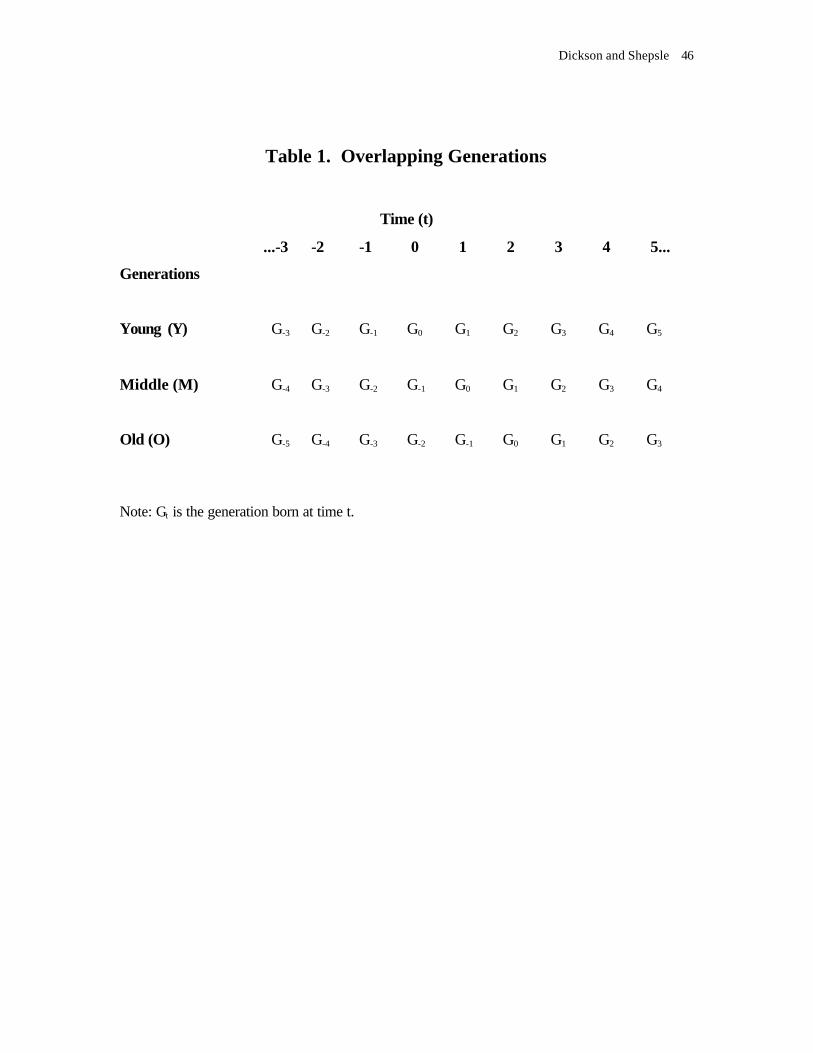
Dickson and Shepsle 46
Table 1. Overlapping Generations
Time (t)
...-3 -2 -1 0 1 2 3 4 5...
Generations
Young (Y) G-3 G-2 G-1 G0 G1 G2 G3 G4 G5
Middle (M) G-4 G-3 G-2 G-1 G0 G1 G2 G3 G4
Old (O) G-5 G-4 G-3 G-2 G-1 G0 G1 G2 G3
Note: Gt is the generation born at time t.

Dickson and Shepsle 47
Seniority
Dependency
Sabbatical
Hobbesian
Figure 1. A graphical representation of different classes of working equilibria. Periods of life in
which individuals work are shaded.
Age

Dickson and Shepsle 48
1 NT N(T-1) + 1/(T-1) N(T-1) + 1
?
All k ? T-1 are equilibria
Some k < T-1 are equilibria
No k>0 is an equilibrium
Figure 2. A graphical representation of the three regimes of Proposition 3.

Dickson and Shepsle 49
FOOTNOTES *Dickson ([email protected]) is a PhD candidate in Government at Harvard University. Shepsle
([email protected]) is Markham Professor of Government at Harvard. An earlier version of
this paper was prepared for the meetings of the Public Choice Society, Charleston, SC, March 10-12, 2000.
We are especially appreciative of John Chant’s comments at that time. A penultimate draft was presented
to the Research Workshop in Positive Political Economy at Harvard. We thank its participants and
especially Macartan Humphreys for detailed, constructive comments. We are also grateful for the
contributions of Rob Van Houweling, a PhD candidate at Harvard who collaborates with us in a larger
project. This larger project is funded in part by a grant to Shepsle from the National Science Foundation
(SBR-9812385). We thank the Center for Basic Research in the Social Sciences at Harvard University, the
Centre for Economic Learning and Social Evolution at University College London, and the Department of
Government at the London School of Economics for providing office space and support. Finally, we are
very appreciative of the excellent remarks and insights of two referees and the editors of JLEO.
1 Note that in the seniority equilibrium an individual’s career switches from one status to another in a
discontinuous manner. This may only be approximated in some empirical contexts where the transition is
more gradual.
2 By “symmetric” we mean that all players of a specific organizational age play the same strategy;
equilibrium strategies are age-specific.
3 This is an adaptation of a model originally presented in Cooper and Daughety (1989).
4 This is an appropriate assumption for a group of fixed size like a legislature, committee, or court. It is
approximately correct for roughly stable groups like bureaucracies and perhaps primitive tribes. The
assumption grows tenuous for groups with highly variable membership.
5 This is clearly a simplifying assumption. In principle, ? could vary with age – capturing either learning or
aging effects – or with calendar date – reflecting temporal changes in the technology of effort. We discuss
these further in the extensions section.

Dickson and Shepsle 50
6 If a member is beyond the kth period of his or her term in the group, then the equilibrium requires no
further contribution, and the continuation value is simply Nk times the number of remaining periods.
7 While this particular punishment regime may seem absurdly severe for many applications, it is
nonetheless useful analytically as a limiting case, since if a grim-trigger strategy cannot sustain cooperative
behavior in equilibrium, then no punishment regime can.
8 Our propositions are special cases of OLG Folk Theorems – see Kandori (1992) and Smith (1992). These
imply that any payoff stream that exceeds individually rational payoffs is sustainable as a subgame perfect
equilibrium. The continuation-value calculation in our results reflects this consideration.
9 The language ties the analysis a bit too closely to the world of labor markets, where “privileged
inactivity” means retirement. In fact, the analysis applies to any situation where the privileged phase
means that the member no longer is required to contribute to the group’s public good but may nevertheless
continue to enjoy it. Thus, elder status in the tribal setting – in effect, the beginning of one’s private life –
captures this idea better than retirement in the labor-market setting.
10 The premise of Claim 2 gives ? ? (P-D)N. Substituting into (2) yields (T-D-1)? ? (P-D)? -1 which holds
if P ? T-1.
11 For example, a tribal village intent upon providing for its common defense probably cannot rely upon
young boys below a certain age to contribute to this enterprise. Nor, perhaps, can it rely upon elderly men
either. This, in turn, suggests that we should not treat ? as invariant with age and experience, and that it is
probably changing cost conditions that require dependency to be taken as constraining. Likewise, even if a
changing ? did not inhibit contributions from the young, the introduction of discounting may well do so. If
future net benefits are discounted steeply enough, a new member of the group might choose to defect early
rather than to have front-ended contributions required. In this case an equilibrium necessarily must not
entail contributions from the (too) young. We will take up the issue of discounting shortly.
12 There is a second complication worth noting briefly. We have implicitly assumed that the equilibrium
specifies not only the number of sabbaticals (N-k), but also the particular periods in which a member is
entitled to take one (e.g., “every seventh period”). Thus, members know that Nk units of the public good
will be produced every period, barring defection. This allows a member to determine his or her defection

Dickson and Shepsle 51
payoff, namely Nk-1. If, on the other hand, a sabbatical practice specifies only the number of sabbatical
periods to which a member is entitled, so that members choose sabbatical dates independently, then the
payoff in any particular period is not know with certainty.
13 In other words, we can think of society as playing a larger game to determine which of the equilibria of
the public goods allocation subgame to adopt. The winning alternative is then an equilibrium both of the
subgame and of the larger game. The identity of the winner will of course depend on the rules of the larger
game.
14 In Figure 3, k=10 is most-preferred by eight of eleven generations. In Figure 4, six of the eleven
generations prefer k=10 most.
15 In this regard, the phenomenon of sabbatical leaves, with which those of us in universities are familiar, is
quite interesting. Initially, the motivation for sabbatical leaves – and the arcane rules in some universities
requiring that they be taken on a regular basis – derived from concerns by boards of trustees about faculty
burnout, not from a desire to allow for a period of intensive research. Effort, in the language of this paper,
grew ever more costly in a cyclical manner, necessitating a break to permit the intellectual batteries to
recharge and the cost of effort to return to an earlier level.
16 We thank Macartan Humphreys for suggesting this line of development.
17 These three regimes of ? were introduced in Proposition 3 and are depicted graphically in Figure 2.