working paper 16 27 - federal reserve bank of cleveland

w o r k i n g

p a p e r

F E D E R A L R E S E R V E B A N K O F C L E V E L A N D

16 27

Spatial Dependence and Data-Driven Networks of International Banks

Ben Craig and Martin Saldías

Working papers of the Federal Reserve Bank of Cleveland are preliminary materials circulated to stimulate discussion and critical comment on research in progress. They may not have been subject to the formal editorial review accorded offi cial Federal Reserve Bank of Cleveland publications. The views stated herein are those of the authors and are not necessarily those of the Federal Reserve Bank of Cleveland, the Board of Governors of the Federal Reserve System, the International Monetary Fund, Bundesbank, or the Eurosystem.

Working papers are available on the Cleveland Fed’s website: https://clevelandfed.org/wp

Working Paper 16-27 December 2016

Spatial Dependence and Data-Driven Networks of International BanksBen Craig and Martin Saldías

This paper computes data-driven correlation networks based on the stock returns of international banks and conducts a comprehensive analysis of their topological properties. We fi rst apply spatial-dependence methods to fi lter the effects of strong common factors and a thresholding procedure to select the signifi cant bilateral correlations. The analysis of topological characteristics of the resulting correlation networks shows many common features that have been documented in the recent literature but were obtained with private information on banks’ exposures. Our analysis validates these market-based adjacency matrices as inputs for the spatio-temporal analysis of shocks in the banking system.

JEL classifi cation: C21, C23, C45, G21.

Keywords: Network analysis, spatial dependence, banking.

Suggested citation: Craig, Ben, and Martin Saldías, “Spatial Dependence and Data-Driven Networks of International Banks,” Federal Reserve Bank of Cleveland, Working Paper no. 16-27.

Ben Craig is at the Federal Reserve Bank of Cleveland. Martin Saldías (corresponding author) is at the International Monetary Fund ([email protected]). The authors are grate-ful for suggestions and comments to conference participants at the Society for Economic Measurement (Chicago), Western Economic Association International Conference (Den-ver), V World Finance Conference (Venice), CEMLA Seminar on Network Analysis and Financial Stability Issues (Mexico City), 8th Financial Risks International Forum (Paris), Financial Risk & Network Theory Conference (Cambridge), INET Conference on Net-works (Los Angeles), and also to seminar participants at the Deutsche Bundesbank, EBS Business School and IMF.

1. Introduction

Financial stability research since the financial crisis has focused on interconnectedness

within the financial system. Developments in the recent financial crisis highlighted the

importance of identifying and understanding the role of specific elements within financial

networks as well as the channels of risk and stress transmission, including those that

are not purely contagion. Ambiguous results of initial theoretical work have emphasized

the need to get a clearer understanding of the functioning of financial networks from

empirical observation. Such an understanding should provide far more than a measure-

ment of simple terms within a clearly understood model. The theoretical literature needs

observation of the actual networks to drive the direction of future investigation. From

a macroprudential policy perspective, a clear understanding of networks’ structures and

functioning in the financial system should provide policymakers with the tools to quickly

react to financial shocks, mitigate risks, and take targeted precautionary actions.

While new empirical work is available, and it often makes use of new bilateral data

within a network, it is hampered by the fact that these data sets are rare, often highly

specific, and usually confidential and hard to access1.

This paper contributes to the empirical network analysis literature in financial stabil-

ity with a method to compute undirected and data-driven correlation networks based on

daily bank stock returns. Using a sample of 418 banks all across the world between Jan-

uary 1999 and December 2014, we apply recently developed spatial-dependence methods

that filter the effects of strong common factors in the correlation across banks and apply a thresholding method to obtain a sparse adjacency matrix, W , that can be used for spatio-

1Recent contributions in this area include Peltonen et al. (2014) for CDS markets, Alves et al. (2015)for insurers’ balance sheet exposures, Alves et al. (2013) and Langfield et al. (2012) for interbank balancesheet exposures, Minoiu and Reyes (2011) for international cross-border bank lending and Iori et al.(2008) and van Lelyveld and Liedorp (2004) for interbank money markets.

2

temporal analysis of shocks across banks in a spatial vector autoregression (SpVAR)or a

Global vector autoregression (GVAR) model, as outlined in Bailey et al. (2015b).

In order to assess the soundness and empirical accuracy of this approach, we analyze

the topological characteristics of the resulting networks and find a number of interesting

common features documented in the recent literature, which were derived from confiden-

tial data sources. In particular, the resulting networks show rich and hierarchical struc-

tures based on but not limited to geographical proximity, small world features, regional

homophily, and a core-periphery structure. This core-periphery structure is adapted from

Craig and von Peter (2014) and applied to a topological structure where domestic (mainly

peripheral) linkages coexist with regional and interregional linkages. All these character-

istics have relevant implications in the way shocks are diffused in the banking system.

We also demonstrate that our results and the performance of the filtering and thresh-

olding methods are robust to random noise resulting from changes in the structure of the

underlying data. Given that our dataset and most others are unbalanced and our filtering

and thresholding method does not depend on a balanced panel structure, we show that

our network structure does not suffer significant distortions from random noise which

would generate spurious correlation. Finally, as a result of the thresholding method, this

approach generates sparse networks that are useful in terms of the spatial modelling as

a regularization method that clearly distinguishes between neighbors and non-neighbors

and allows analysis of large scale datasets.

The rest of the paper is organized as follows. Section 2 provides a concise review of

models of networks based on stock market information in order to provide a context for

this research. An empirical application is thoroughly described in Section 3. Results are

provided in Section 4 and conclusions and discussion of future research are summarized

3

in Section 7.

2. Empirical models of financial networks

This section first reviews the empirical models of networks that have been developed from

stock market information and then describes the general features of the spatia-dependence

approach to network analysis that is used in this paper. Among the former models, the

most popular ones are grouped into graph theory methods and into multivariate time

series models. They differ in terms of the network structure assumed and their use of

model shocks within the network.

In particular, graph theory methods have well defined but rigid network structures.

Multivariate time series analysis methods allow for flexible network structure, generally

producing dense networks, but they put less emphasis on the characteristics and impli-

cations of the network’s structure on the transmission of shocks across nodes.

In both cases, the presence and importance of common factors are analyzed superfi-

cially, which is what takes us to the spatial-dependence approach. This literature belongs

to the panel vector autoregression (PVAR) literature 2 and hence allows us to easily iden-

tify and model shocks and their transmission. This approach also allows to introduce

the concept of spatial proximity in order to analyze the extent to which the strength of

interdependence is a result of common factors and whether it can be filtered out.

2.1. Graph theory methods

Generally, the existing methods using graph theory to extract an undirected network of

relevant interactions from a complete correlation matrix are based on two graph the-

ory concepts, namely Minimum Spanning Trees (MSTs) and Planar Maximally Filtered

2See Canova and Ciccarelli (2013) for a comprehensive review of the PVAR literature and alternativeapproaches.

4

Graphs (PMFGs). The application of MSTs is originally outlined in Mantegna (1999)

and consists of obtaining a subgraph of N − 1 links that connect all N nodes of the net-

work by minimizing the sum of the edge distances starting from the possible N(N − 1)/2

edges of a complete network. The method transforms each element ρij of the correlation

matrix into a distance metric3 and applies Kruskal’s algorithm or Prim’s algorithm to

find the MST.

As this method is generally applied to a set of constituents in a stock market index,

the resulting MST shows a well defined topological arrangement that allows us to group

the network nodes into industries, sectors or even sub-sectors and to establish a hierarchy

with an economic meaning4. This implies that the MST grouping is consistent with the

existence of underlying factors affecting the stock returns such as investors’ investment

focuses and economic activity. However, MSTs do only allow for single links, and thus

the formation of cliques or non-connected components of the network is not possible. As

a result, the MST becomes a simple but very restricted topological structure in terms of

modeling shock transmission channels between nodes.

Planar Maximally Filtered Graphs (PMFGs) are introduced in Tumminello et al.

(2005)5 and partially address the MST constraints by allowing for slightly richer sub-

structures, including cliques and loops of up to a predefined and small number of nodes.

PMFGs produce a network with 3(N − 2) edges, contain an MST as a subgraph and

share its hierarchical organization. They do however keep the completeness of the net-

work and, as in the MST, the resulting dependency structure determines by construction

the distribution of centrality or clustering measures across nodes in the network and hence

3The distance measure is defined as di,j =√

2 (1− ρij), which fulfills the three axioms of a metric,namely: 1) di,j = 0 if and only if i = j 2) di,j = dj,i and 3) di,j ≤ di,k + dk,j . Other relevant referencesalong these lines can be found in Bonanno et al. (2004) and Tumminello et al. (2010)

4When applied to stock indices and currencies or to stocks in different markets, MST groups nodesaccording to geography.

5See also Aste et al. (2005); Pozzi et al. (2013); Tumminello et al. (2010) and references therein.

5

their role as shock transmission channels. Recent developments in this literature include

models with network dynamics, more flexible community detection, the use of partial

correlations. These and alternative methods establish a distance metric and hierarchical

structure which can explain how shocks are transmitted.

2.2. Time series approach

The contributions from multivariate time series methods to network analysis are even

more recent. The resulting networks are mainly directed networks estimated from causal-

ity relationships or spillover effects. Regularization methods are often applied in order

to deal with large datasets, to induce sparsity and as an econometric identification tool.

These models also allow for dynamics in the interdependencies and tend to only include

observable factors to control for macrofinancial common factor exposures. Being at an

early stage, however, they focus on methodology rather than concentrate on the analysis

of the network topology.

For instance, Diebold and Yilmaz (2014) build and analyze static and time-varying

directed and complete networks based on variance decompositions from a vector autore-

gression (VAR) model applied to daily stock returns and realized volatilities of a relatively

small number of financial companies6. In Billio et al. (2012) network edges are formed

by linear and nonlinear Granger-causal relationships between financial institutions, i.e.

hedge funds, banks, broker/dealers, and insurance companies, for different sample sub-

periods and rolling windows. The authors provide a summary of network measures and

show robust results to the inclusion of observed common factors affecting the bilateral

relationships. The resulting networks are overall very dense and complete, especially in

crisis periods.

6Diebold and Yilmaz (2015) covers this approach and provides additional applications to macrofi-nancial data.

6

Hautsch et al. (2014a,b) model static and time-varying tail risk spillovers between

banks and insurance institutions. They use a LASSO-type quantile regression to select

the relevant risk drivers across banks and thus define the directed network’s edges and

gauge their systemic impact and changing roles in time. The authors also control for

observable common tail risk drivers and find substantial persistent country-specific risk

channels. Also recently, Barigozzi and Brownlees (2013) characterize cross-sectional con-

ditional dependence and define the links of a network using long-run partial correlations.

This model is based on a vector autoregressive representation of the data-generating

process as in Diebold and Yilmaz (2014) but turns to LASSO to estimate the long-run

correlation network. This approach takes into account contemporaneous and dynamic

aspects of network connectedness which allows us to deal with large dimensional data. In

an empirical application to 41 blue-chip stock returns, the authors control for only ob-

servable common factors using a one-factor model but obtain a relatively sparse matrix

with interesting features, including unconnected nodes and clustering.

2.3. Cross-sectional and spatial dependence in panels

Even though some work described in the previous section does explicitly account for ob-

servable common factors, empirical models of financial networks largely overlook the role

of spatial dependence in the data and its implications for interdependence. In this lit-

erature, relationships between spatial units include both purely spatial dependence and

the effect of common factors. If common factors are strong, e.g., aggregate shocks or

pure contagion, as defined in Chudik et al. (2011) and Bailey et al. (2015a), resulting

interdependences are misleading. As a result, strong common factors need to be detected

and removed from the data in order to highlight the purely spatial dependence.

Spatial dependence in a broad sense is illustrated in Conley and Topa (2002); Conley

7

and Dupor (2003); and more recently analyzed in depth in Chudik and Pesaran (2013b).

In the economic sense and applied to the banking sector and its stock market returns,

spatial proximity is related to a number of features, including similarity of business lines,

common balance-sheet or market exposures, common geographical exposures, accounting

practices, or technological linkages. Hence, removing strong common factors from bilat-

eral correlations highlights these features.

Bailey et al. (2015b) extend the cross-sectional dependence analysis from panel data

to network analysis by applying a model of spatiotemporal diffusion of shocks to house

prices. In this setting, the authors choose a hierarchical model based on geographical

areas and introduce a method to filter the strong common factors from the data and

establish the significant correlations that create the adjacency matrix (Bailey et al., 2014).

The authors compare their results to an exogenously defined adjacency matrix, but the

network properties become less relevant in their analysis. They do however provide the

motivation to apply this method to a different context and to stress its applicability in

financial stability analysis.

3. Empirical application

Following Bailey et al. (2015b), the extraction of the bank network based on correlations

comprises two steps, the removal of strong factors from the returns series; and the regu-

larization or thresholding. First, the potential existence of strong factors in the data is

evaluated using the cross-section dependence (CD) tests developed in Pesaran (2015)and

Bailey et al. (2015a). In case the null of weak dependence is rejected, sequential esti-

mation of common factors is conducted using principal components. Once the CD tests

confirm that the strong common factors have been purged, a correlation matrix is com-

puted to apply thresholding.

8

The thresholding step selects the correlation coefficients, ρij, among weakly-dependent

residuals that are statistically different from zero at a given significance (5%) level from

all possible N(N − 1)/2 elements of the correlation matrix using the Holm–Bonferroni

method. Finally, a data-driven undirected network, W, is obtained which can be analyzed

in terms of its topological properties. A detailed description of these steps and the

database is presented below.

3.1. Sample and preliminary data treatment

The sample consists of daily log-returns between January 1999 and December 2014 (4173

observations) of 418 banks located across 46 countries from three large geographical re-

gions (Table 1). In particular, the EMEA (Europe, the Middle East and Africa) region

includes 26 countries, Asia includes 12 and the Americas has 8. Due to the particularities

of each country’s banking sector and stock market, some countries, such as the USA,

Japan, or India, have many more banks in sample than countries where banks are not

as extensively listed, such as Germany or Mexico, or where the banking sector is highly

concentrated, like Singapore, Belgium, or the Netherlands.

The sample is unbalanced at both ends as it includes delisted, bankrupt, acquired

or merged, and also newly listed banks. Before the defactoring step, we first transform

the log-returns into series with zero means and unit variances to reduce the scale effects

in the data. This detail is relevant in two ways. First,it allows us to keep the effect

of the stock price movements of new or defunct banks in terms of the common factors

filtering and as a possible source of a strong dynamic factor (Chudik and Pesaran, 2013a).

Second, it avoids possible significant omissions due to survivorship bias that may affect

the resulting structure of the network. For instance, much of the stock market analy-

sis focused on Bear Stearns and (then on Lehman Brothers during 2008) and how their

stock price developments were transmitted as global factors to other markets. Similarly,

9

newly listed large Chinese banks have quickly become the largest in the world by market

capitalization and in terms of their regional and global relevance.

Then we the introduce standard normal random noise into the missing data to obtain

a block structure while keeping independence across the draws. This step brings correla-

tions toward zero when a pair of series have a minimum or no overlap, which is equivalent

to assuming those correlations are zero. Although Bailey et al. (2015b) do not rely on

the block structure of the data or on the length of the time series, some of the features

from the asymptotic behavior of eigenvalues rely on the block structure of the data matrix.

As the banks are located all over the world, the sample has to be robust to non-

synchronous market trading, which may induce spurious correlations and emphasize the

role of the countries where news arrives first and exacerbates regional clustering artificially

(Lin et al., 1994). Accordingly, all log-returns from Asian banks have been lagged one

trading day.

[Insert Table 1 here]

3.2. Removal of strong factors

The presence of strong cross-sectional dependence is modeled using unobserved common

factors, i.e. a principal components analysis (PCA), which provides a more flexible ap-

proach to capturing the strong common factors. Alternatively, cross-sectional averages

at national and regional levels could be used as in Bailey et al. (2015b) and outlined in

Pesaran (2006). This latter approach embeds hierarchical spatial and temporal relation-

ships, where the hierarchy is exogenously predetermined.

Although a geographical hierarchy is likely to be present in the case of stock returns,

as referred to in Section 2.1, the interlinkages in the banking sector go beyond the national

10

and regional boundaries and thus include other forms of spatial dependence across bor-

ders. In addition, the definition of regions has some degree of subjectivity that can affect

de-factoring and thus the resulting network structure7. Finally, the heterogeneous dis-

tribution of banks by nationality may also introduce some bias in the defactoring process.

The weakly dependent residuals are obtained from the following regression using ro-

bust methods to control for outliers8.

yit = αi + β′ift + uit (1)

where yit is the daily log-return of bank i on trading day t9. ft are the principal com-

ponents extracted through PCA with associated factor loadings βi = (βi1, βi2, . . . , βiN)′.

The de-factored log-returns are then given by the following equation:

uit = yit − αi − β′ift (2)

The cross-sectional dependence tests described below set the number of principal compo-

nents ft to be extracted from the stock returns. In this application, there is no prior to

the maximum number of factors.

3.3. Testing cross-sectional dependence

The cross-sectional dependence test, developed in Pesaran (2015), is based on pairwise

correlation coefficients, ρij, of regression residuals from equation 2 for a given number of

7As a robustness check, de-factoring was also conducted using cross-sectional averages at national,regional and aggregate level. The resulting residuals did not show enough evidence of being stripped fromthe strong dependence and the networks obtained under different definitions of regions showed unstabletopological properties.

8The robust estimation method is outlined in Andrews (1974).9Prior to the PCA estimation, the banks’ normalized daily log-returns yit were seasonally adjusted

using daily dummies and an intercept.

11

factors10.

CDP =

√2

N (N − 1)

(N−1∑i=1

N∑j=i+1

√Tij ρij

)(3)

Pesaran (2015) shows that the CDP implicit null depends on the relative rate at

which T and N expand. Under an implicit null of weak cross-sectional dependence,

CDP → N(0, 1), and this rate α, defined as the exponent of cross-sectional dependence

(Bailey et al., 2015a), is α < (2 − ε)/4, as N → ∞, such that T = κN ε for some

0 ≤ ε ≤ 1, and a finite κ > 0. In particular, when the null of weak dependence is not

rejected, 0 ≤ α < 12. When the null of weak dependence is rejected and 1

2< α < 1,

Bailey et al. (2015a) show that α can be estimated consistently using the variance of

cross-sectional averages, and this paper follows this procedure in order to ensure the

dataset is stripped from strong common factors.

3.4. Thresholding and data-driven correlation network W

Based on the weakly dependent residuals from a subset of the whole sample,11 the cor-

responding correlation matrix turns into a data-driven correlation network, W, through

a multiple testing of the significant correlation coefficients, ρij. In order to tackle the

potential dependence among tests and to control the familywise error rate (FWER), the

Holm-Bonferroni multiple comparison test uses the elements of the correlation matrix

and corresponding p-values. Holm-Bonferroni is a conservative test and therefore ensures

a sparse network, W.

In practice, the test consists of sorting the m = N(N−1)2

p-values P1, . . . Pm and asso-

10ρij =

∑t∈Ti∩Tj

(uit−¯ui)(ujt−¯uj) ∑t∈Ti∩Tj

(uit−¯ui)2

1/2 ∑t∈Ti∩Tj

(ujt−¯uj)2

1/2 , where uit and ujt are residuals from equation 2

11In particular, 31 banks from the initial 418 are excluded from the thresholding step as they weredelisted due to bankruptcy, M&A, etc. and their relevance for the network properties is less significant

as for the de-factoring. Consequently the network W analyzes only banks that are listed at the end ofthe selected time span.

12

ciated hypotheses of correlation significance, H1 . . . Hm, in order of smallest to largest.

Starting from P1 and for a significance level of 5%, if P1 ≤ αm

, the associated correlation

is significantly different from zero, and we move to P2 and compare it with αm−1

. The test

continues in this fashion until it fails to reject the hypothesis of significance, i.e., Pk ≥ αm−k

for k ≤ m, where k is the stopping index. All elements of the correlation matrix from that

point on are set to zero, and the first k−1 elements are set to one and form the W matrix.

3.5. Network analysis

Based on the W network, we estimate a number of measures that characterize it as an

undirected network and describe the properties of its nodes. In addition, we analyze

three sub-networks based on specific properties of the dataset. First, we construct three

sub-networks based on the regions of origin of the banks in the sample, two sub-networks

according to positive (complementary) and negative (substituting) connections and a sub-

network that focuses on cross-border relationships.

Based on the W network, we estimate a number of measures that characterize it

as an undirected network and describe the properties of its nodes. Then, we construct

three sub-networks based on the regions of origin of the banks in the sample and two

sub-networks that focus on cross-border relationships. In particular, we construct three

subnetworks based on the regions of origin of the banks in the sample (WEMEA, WAsia

and WAmericas) and two sub-networks that focus on cross-country (WCross−country) and

cross-regional relationships (WCross−region). In addition, each network is analysed with

respect to two sub-networks according to positive (complementary) and negative (substi-

tuting) connections.

As for network metrics,12 we compute network density and measures of degree dis-

12See Boccaletti et al. (2006) and Jackson (2008) for definitions and general interpretation of these

13

tribution (average degree, maximum degree, average neighbor degree, assortativity and

clustering), distance (diameter, average path length) and other complementary metrics.

Finally, a tiering analysis is conducted based on the method outlined in Craig and von

Peter (2014) in order to detect whether there is a hierarchical structure in the network that

makes transmission channels work through a core-periphery structure. In applications

reviewed in Section 2, in spite of the fact that networks are very dense, core-periphery

structures are quite common. In a sparse network context, this result has important

implications in terms of the channels of transmission of shocks, as it identifies those banks

that connect countries or regions and highlights their role as central in the network.

4. Results

4.1. Aggregate network W

Before turning to the topological properties of network W and in accordance with Section

3.3, CD tests were conducted to the balanced panel of seasonally adjusted and standard-

ized log-returns and sequentially to residuals from equation 2 for an increasing number

of factors until strong cross-sectionally was removed. The CDP statistic for the data

without any defactoring (2485.1) clearly rejects the null of cross-sectional weak depen-

dence compared to a critical value of 1.96 at the 5% significance level, pointing to the

presence of strong common factors. The corresponding bias-free estimate of the exponent

of cross-sectional dependence (standard error in parenthesis) from Bailey et al. (2015a)

is α = 0.996(0.022). The sequential inclusion of factors stopped at three, yielding a CDP

statistic of -1.82 (p − value = 0.0683), which ensured the weakly cross-section depen-

dence that allows us to proceed to thresholding. The associated bias-free estimate of the

exponent of cross-sectional dependence was reduced to α = 0.831(0.016), still above the

borderline value of 0.5 but way below the initial estimate.

measures.

14

The resulting network, W, is presented in a sparsity plot in Figure 1, where a square

represents the significant correlation coefficient between a given pair of banks. The square

colors represent the strength of the relationship.13 The banks are sorted first by region

and then by country in alphabetical order as shown in Table 1. As expected, the Holm-

Bonferroni method produced a sparse adjacency matrix with density of 0.0654, which

corresponds to 4,885 edges out of a total of 74,691 possible bilateral relationships. 14

[Insert Figure 1 here]

The network is not fully connected, as six banks are isolated from the rest. 15 After

removing these nodes, the resulting network diameter is 8, while the average path length

is 2.84 and the clustering coefficient is 0.5281, which is much larger than the network

density and the clustering coefficient of a random Erdos-Renyi graph of comparable den-

sity16 (see Table 2).

The degree distribution of the network is heavy tailed. Altogether, this provides ev-

idence of a small world network, which is a common feature found in recent research on

networks based on bank exposures (Alves et al., 2013; Peltonen et al., 2014). This result

is relevant if this network is used as an adjacency matrix in a spatial model of shock

transmission, as it means that second round and feedback effects of a shock to a given

bank are likely to propagate quickly to any other bank in the network.

13In particular, for both the positive and negative scales, weak, medium strong correlations correspondto correlation coefficients below one third, between one and two thirds, and above two thirds, respectively.

14Even after de-factoring, the correlation matrix that generates W shows significant correlation coeffi-cients in the range of -0.22 and 0.76 with a ±0.077 correlation defined by the chosen threshold significancelevel.

15The existence of non-connected nodes in filtered correlation networks means that shocks from and tothese nodes are not direct but take place through the common factors among stock returns. In this par-ticular case, these are banks from Austria, Switzerland, Finland and Japan(3) that have a predominantlydomestic activity.

16For a simulated Erdos-Renyi graph of size 387 and density of 0.0654, both average path length (2.10)and clustering coefficient (0.069) are smaller.

15

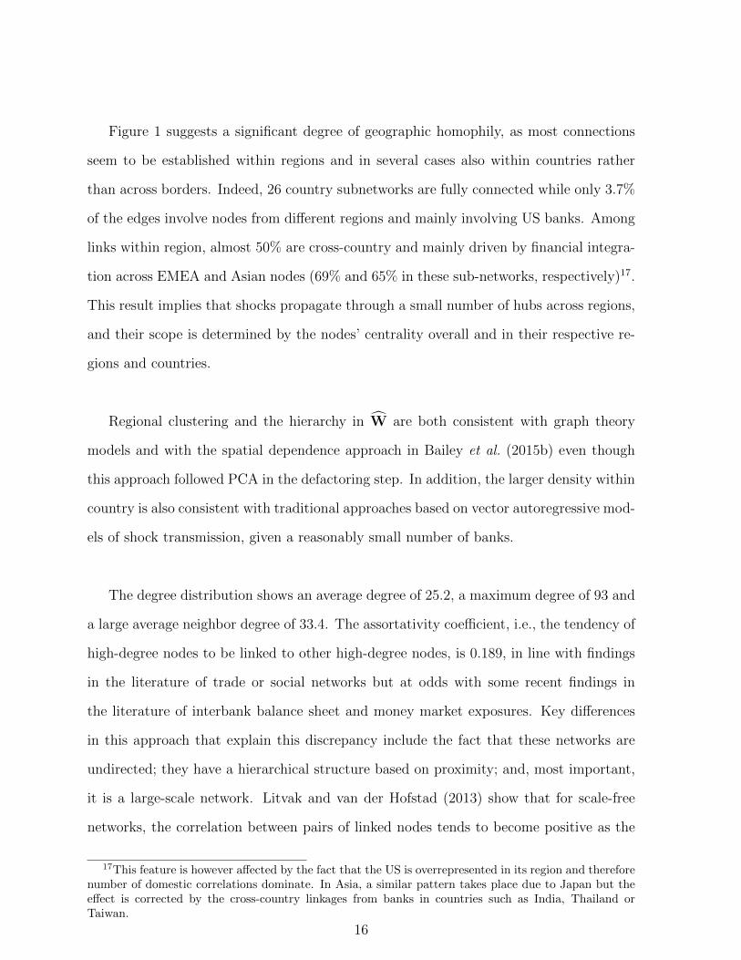
Figure 1 suggests a significant degree of geographic homophily, as most connections

seem to be established within regions and in several cases also within countries rather

than across borders. Indeed, 26 country subnetworks are fully connected while only 3.7%

of the edges involve nodes from different regions and mainly involving US banks. Among

links within region, almost 50% are cross-country and mainly driven by financial integra-

tion across EMEA and Asian nodes (69% and 65% in these sub-networks, respectively)17.

This result implies that shocks propagate through a small number of hubs across regions,

and their scope is determined by the nodes’ centrality overall and in their respective re-

gions and countries.

Regional clustering and the hierarchy in W are both consistent with graph theory

models and with the spatial dependence approach in Bailey et al. (2015b) even though

this approach followed PCA in the defactoring step. In addition, the larger density within

country is also consistent with traditional approaches based on vector autoregressive mod-

els of shock transmission, given a reasonably small number of banks.

The degree distribution shows an average degree of 25.2, a maximum degree of 93 and

a large average neighbor degree of 33.4. The assortativity coefficient, i.e., the tendency of

high-degree nodes to be linked to other high-degree nodes, is 0.189, in line with findings

in the literature of trade or social networks but at odds with some recent findings in

the literature of interbank balance sheet and money market exposures. Key differences

in this approach that explain this discrepancy include the fact that these networks are

undirected; they have a hierarchical structure based on proximity; and, most important,

it is a large-scale network. Litvak and van der Hofstad (2013) show that for scale-free

networks, the correlation between pairs of linked nodes tends to become positive as the

17This feature is however affected by the fact that the US is overrepresented in its region and thereforenumber of domestic correlations dominate. In Asia, a similar pattern takes place due to Japan but theeffect is corrected by the cross-country linkages from banks in countries such as India, Thailand orTaiwan.

16

network size grows.

Along these lines, Figure 2 shows the degree and average neighbor degree distribution

for the complete network and also for the regional subnetworks, where the corresponding

regions are displayed in different colors. Overall, the linear correlation between the nodes’

degree and average neighbor degree is positive for both the complete network (0.5988) and

the subnetworks. In particular, the correlation coefficients are 0.4733, 0.5396, and 0.6722

for the EMEA region, Asia, and the Americas, respectively. This evidence reinforces the

previous findings on the assortative characteristics of the network, and the differences in

association provides some additional insights about the regions.


A large degree concentration among the most connected nodes points to the rich-

club phenomenon, i.e., the existence of highly connected and mutually linked nodes, as

opposed to a structure comprised of many loosely connected and relatively independent

sub-communities, as defined in Colizza et al. (2006). Indeed, the rich-club coefficients18

for nodes with a degree over 40, 50, and 60 are 0.3370, 0.4273, 0.8693, respectively, which

means hubs are tightly connected but also are likely to serve as bridges across borders.


4.2. Properties of Regional Subnetworks

The regional subnetworks, presented in Figures 3, 4 and 5, show stronger small-world

properties due to the higher density across countries, and thus they reinforce those from

the W network. Columns 2 to 4 in Table 2 summarize them. Regional subnetworks

are at least twice as dense as the aggregate network, W. Their diameters are smaller

in every case, their average path lengths are shorter, and their clustering coefficients are

18In particular, this measure computes the fraction of edges actually connecting those nodes out ofthe maximum number of edges they might possibly share.

17

larger. As a corollary, all regional networks present positive assortativity, especially in the

EMEA region, and a rich-club analysis shows coefficients of 0.5654, 0.3951, and 0.5801

for EMEA, Asia, and the Americas for a degree higher than 20.19

[Insert Figures 3, 4 and 5 here]

The sub-network WCross−country includes all nodes in network W with at least one

edge with a bank in a different country and contains subnetwork WCross−regional, which

keeps only banks with cross-regional relationships. They are displayed in Figures 6 and

7 and, as in the regional subnetworks, these networks reinforce the topological properties

of the aggregate network, W. In particular, they have stronger evidence of a small-world

network, rich-club, and positive assortativity. The sparse distribution of links across

regions described above explains the large drop in size from subnetwork, WCross−country

(316) to WCross−regional (140). As several nodes with only domestic links are excluded

in the cross-regional subnetwork WCross−regional, its blocky structure is attenuated and

therefore its assortativity coefficient increases significantly compared to the cross-country

subnetwork WCross−country.

[Insert Figures 6 and 7 here]

5. Regions and the International Core

Having identified a blocky network structure with low density, low diameter, high degree

concentration, positive assortativity but strong regional homophily in W, the importance

of a small set of nodes in linking countries and regions needs to be analyzed in depth.

We turn therefore to a tiering analysis modifying the core-periphery model in Craig and

19If the higher degree is set to 30, the coefficient reaches 0.5952 in Asia, 0.7058 in the Americas andreaches 0.7749 in the EMEA region

18

von Peter (2014).20

The correlation networks analyzed in the previous section embed some of the essen-

tial international banking structure, particularly in the structure between a bank with

cross-border connections and banks that lie within a particular region or country. By

allowing regional cross-sectional strong dependence to persist while estimating interbank

linkages, we emphasize links that are created by banks within a region that are tied to a

national market, which is indistinguishable from the cross-sectionally weakly dependent

ones estimated in the international links.

However, by purging the regions of their regional strong factors, we would eliminate

those correlations that are implicit in an extraregional bank with ties to the region, which

is crucial to our understanding of international banking networks. This presents a co-

nundrum that is best resolved after the network has been computed, as the network is

analyzed.

We demonstrate this with estimates of the core-periphery structure of international

banking. Estimating a core using the method in Craig and von Peter (2014) directly

from the international correlation networks described above may lead to a misleading

core that overemphasizes domestic links. We therefore redefine and reestimate in this

section the core-periphery structure with a new measure that correctly allows domestic

links to exist within the periphery. This new structure leads to a much more revelatory

structure that is in line with the intuition about money-center banks, R-SIBs, and G-SIBs.

The core-periphery structure of Craig and von Peter (2014) is based upon the adja-

cency matrix of unweighted links, similar to network W, except in that it can be estimated

20Traditional analysis of centrality in this case is misleading as measures such as betweenness, eigen-vector or Katz-Bonacich centrality do not have consistency and their ranks are distorted by the structureof the network and regional subnetworks.

19

from both directed and undirected networks. The estimated structure depends upon an

ideal where within the core, all links are made between the core and periphery, and at

least one link occurs between a core bank and a periphery bank, and further, within

the periphery, there are no links. An example of an ideal core-periphery structure is in

Figure 8, where the top-left CC block includes three banks that are fully connected. The

off-block-diagonal blocks, CP and PC, have at least one link from each core bank to the

periphery. Finally, and most importantly for our discussion, the PP block illustrates no

links between the periphery banks.


The repair in this paper lies in redefining the core so that links within a country or

region are not penalized and prevented from being in an idealized periphery-to-periphery

block. To illustrate, Figure 9 shows an adjacency matrix where several countries are

indicated by the labels. In this ideal, the ones in the PP block are not penalized because

they represent domestic or regional links. However, the same ideal is observed in the

other blocks: core banks are required to interact tightly with other core banks, and the

periphery-to-core and core-to-periphery blocks are required to be column regular and row

regular respectively. Deviations from the ideal are penalized according to the same loss

function for the PP, CP, and PC blocks as for the standard core-periphery model, while

deviations from the ideal in the PP block of no links are penalized only if the links are

cross-border.


Table 3 reports the results of the estimation of the core structure of Craig and von

Peter (2014) (original core) and the alternative structure (new core) on the W network

and the three regional subnetworks. The core banks are then split (in columns) by com-

munities, as defined by the Louvain algorithm (Blondel et al., 2008), in order to add

20

additional information about the interconnectedness among core banks.

For the complete network W , the original core comprises 49 banks from the three

regions that also make up the three communities found by the Louvain algorithm. As the

original core-periphery algorithm does penalize periphery-to-periphery connections, the

number of core banks is larger and several Asian banks21 are included in because they

have simultaneously high domestic density and significant links to other international

banks, mainly American SIFIs. Core banks are therefore not a complete subnetwork and

shows some sparsity among detected communities (see Figure 10). American banks stand

out as the hubs linking not only core banks from EMEA and Asia but also linking regions.

In addition, 11 out of the 17 identifies American core banks are SIFIs as listed by the

FSB22.

[Insert Figures 10, 11 and 12 here]

We computed two sets of new core banks for the W network. The first set does not

penalize the periphery-to-periphery links if they belong to the same country. This new

core and is displayed in Figure 11. It is a subset of the former and includes 39 banks. In

contrast to the original core, no US banks are represented as the strong domestic density

and large domestic subnetwork exclude them from the core. However, several features

stand out. First, the core is more densely connected and positive correlations dominate.

Second, a more preeminent role is given to EMEA banks while new players emerge in the

Asian region, including Australian banks. Third, the Asian banks are divided into two

tightly connected communities that go beyond national borders..

Finally, the third definition of core allows does not penalize links if they belong to the

same region. The resulting new core, displayed in Figure 12, is therefore much smaller

21Mainly Thai and Indian banks, which however are considered systemically important institutionsdomestically.

22See details at http://www.fsb.org/wp-content/uploads/r_141106b.pdf

21

and comprises only 25 American banks. The loss function in this case is very small, which

is not surprising because all periphery intraregional links contribute marginally to the loss

function. This suggests that the US banks have a key role in intermediating across the

globe between regions, especially given that they still tend to rely on domestic funding

for their intermediation. As in the previous case, this set of core banks are largely a sub-

set of the former and mainly includes SIFIs. This core is almost a complete subnetwork

although there is no dominance of negative or positive correlations.

As in the case of the complete network, core composition applied to regional sub-

networks does not change significantly across models, especially because the countries’

networks sizes are less heterogeneous. There is only an alternative definition of cores

that does not penalize intra-country links to take place in the periphery. Well known

SIFIs and R-SIBs link countries within regions and show their importance as channels of

transmission regionally. These findings reinforce their systemic importance both globally

and regionally and provide support to our findings as a method to identify SIFIs using

correlation networks and tiering analysis.


6. Robustness Checks: Interconnectedness Driven by Random Noise

This robustness check applies the theory of random networks to analyze whether some

links in our network from weak cross-sectional dependent data could have been generated

by random noise. The methodology described in Section 3 is based on the successive

removal of factors that create strong cross-sectional dependence and that are often asso-

ciated with the largest principal components of the variance-covariance matrix, until our

tests indicate that weak cross-sectional variation is sufficient to be detected. However,

this procedure does not remove noise, which can generate links randomly, nor detect their

presence and importance.

22

The theory of random networks has a rich literature on noise reduction, where the

noise appears in independent observations that indicate correlations randomly. This

literature is based on Edelman (1988), Bowick and Brezin (1991), Litvak and van der

Hofstad (2013) and Sengupta and Mitra (1999) and applied to finance by Laloux et al.

(2000), whose notation we follow. If we have N banks with T observations of independent

normalized returns with mean zero and variance one, stacked into an NxT matrix M , then

the estimated correlation matrix is C = 1TMM ′, where the prime notation just denotes

the transpose. The estimated correlation matrix C has some very useful properties when

N and T both get large. If Q = TN≥ 1 is fixed, then as N →∞, T →∞, the density of

the probability of eigenvalues, f(λ), goes to the following function:

f(λ) =Q√

(λmax − λ)(λ− λmin)

2πλ(4)

where:

λmaxmin =Q+ 1

Q± 2

√1

Q(5)

This structure suggests that we look at those nodes which depend on variation that is

only present in the range of those eigenvalues where random noise could have produced it

and identify them. Our experiment consists of identifying a critical eigenvalue such that

random matrices with uncorrelated noise will generate eigenvalues lower than this level,

λmax, and then of obtaining the links that are generated by the variation entirely in this

region.

This ideal result differs from our matrix of correlations because we have a finite sample

size, which can be analyzed using the results of random matrices that calculate the rate

of convergence to the limiting density, as presented in Bowick and Brezin (1991). The

second difference we analyze using Monte-Carlo methods to see by how much a matrix

with a similar structure to ours differs from the limiting distribution implied by equation

23

4.


The Monte-Carlo experiments are reported in Figure 13 where the maximum eigen-

value distribution is shown. The eigenvalue distribution is very tightly distributed around

2.03. Any bandwidth that deletes all eigenvalues less than 2.2 will throw out noise in all

but a small fraction of the cases. Second, this represents a sample size value of Q that

is much smaller than our actual set of observations. To be more precise, if we were to

calculate Q naively from the size of our block, then Q = 4123387

= 10.65, which the theory of

random matrices would imply a maximum λ sharply distributed at 1.707. If, instead, Q is

calculated at the average value of T for our sample, which accounts for the missing values,

then Q = 3781387

= 9.77, which our theory would imply a maximum λ sharply distributed at

1.742. Instead, our observed maximum has a distribution that is only somewhat sharply

focused on 2.03, which is what the theory would predict for a sample T in a block sample

of around 2,150 implied by a Q = 5.56. Thus, by losing only 10% of our observations, we

are gaining noise that is equivalent to a reduction of 43% of our sample if this reduction

had been in block format. Going to an unbalanced sample is costly in terms of random

noise.

Having said all of this, our results were similar whether we used the cutoff points

implied by either the balanced or unbalanced panel. When we remove the information

of the lower eigenvalues from the sample our estimates of the correlation coefficients are

much more tightly focused. This implies is that the upper eigenvalues alone given corre-

lation coefficients that reject the value of zero given our significance level of 0.05 for very

many of the correlations. The implied networks have a density of nearly 0.5, because by

assuming that the lower eigenvalues contain only noise, we essentially assume that all

correlation measured in the upper eigenvalues is significant because it is lacking in this

noise. The resulting network is so dense as to be meaningless. As with the work cited24

above for random matrices as applied to the case of portfolio analysis, the information

included in the lower eigenvalues contains both noise and meaningful information that

should not be removed.

Instead, we ask an alternative question in exploring the information contained in the

lower eigenvalues, i.e. those eigenvalues that are less than the cutoff for the balanced panel

design. We ask which links in our network could be generated only by that information

contained in the set of eigenvalues that could be random noise. In other words, if A is

the set of links generated by the information in these eigenvalues (given the information

that could be generated by noise alone, which of the links are significant by our test) and

B is the set of links implied by our sample, what is the set A ∩ B. These are the links

in our networks that could have been generated solely by noise. We ask the question of

whether these are key links in our networks. We find that the number of these links is

small, and we also find that they are not key to any of our findings. In fact, these links

are scattered randomly across our networks with no clusters, with the small exception

of a cluster of seven links that correspond to middle eastern banks. These links do not

affect any of our reported results. Noise alone is not driving our conclusions.

7. Concluding Remarks

This paper outlines a method to compute undirected data-driven networks based on bank

stock returns of 418 banks all across the world between January 1999 and December 2014.

We use spatial-dependence methods that filter the effect of strong common factors and

obtain a large network and three regional subnetworks. The resulting networks show a

number of interesting topological properties when compared to other emerging approaches

in the literature and serve as a market-based adjacency matrix for a panel-data type of

analysis of shocks across banks in a spatial vector autoregression (SpVAR) or a Global

vector autoregression (GVAR) model. Our results provide valuable input into the anal-

25

ysis of contagion from a financial stability perspective. Networks embed a number of

characteristics that are important drivers in the recent financial-stability literature, and

our construction relies on public information rather than on confidential sources.

In particular, the networks and subnetworks show rich and hierarchical structures, in-

cluding geographical clustering, nonconnected nodes, sparsity, or large cliques. In general,

their sparsity or low density is a result of the Holm-Bonferroni method of thresholding, a

method that proves useful in terms of the spatial modeling as a regularization that clearly

distinguishes between neighbors and non-neighbors. The regularization technique is also

robust to other regularization methods. The network and subnetworks also have a very

clear hierarchical structure based on but not limited to geographical proximity.

All networks show small-world properties, which situates this method in line with

findings in recent research on networks based on actual banks’ exposures to different as-

set classes. This feature means that second-round and feedback effects of a shock to a

given bank are likely to propagate quickly and to reach any other bank in the network.

We also find a significant degree of regional homophily, as most connections seem to be

established within regions and intensively within countries. There is also evidence of a

rich-club phenomenon, where highly connected nodes are also mutually linked.

Finally, a joint centrality and tiering analysis of the networks shows evidence of a

core-periphery structure, also in line with recent empirical findings. In particular, a rel-

atively small number of banks serve as bridges for connections between banks in their

regions and between banks across regions.

26

References

Alves, I. et al. (2013), “ The European interbank market ”, Occassional Papers 2, Eu-

ropean Systemic Risk Board.

Alves, I., Brinkhoff, J., Georgiev, S., Heam, J.-C., Moldovan, I. and Scotto

di Carlo, M. (2015), “ Network analysis of the EU insurance sector ”, Occassional

Papers 7, European Systemic Risk Board.

Andrews, D. F. (1974), “ A robust method for multiple linear regression ”, Technomet-

rics, vol. 16 no 4: pp. 523–531.

Aste, T., Di Matteo, T., Tumminello, M. and Mantegna, R. N. (2005),

“ Correlation filtering in financial time series ”, in Abbott, D., Bouchaud, J.-P.,

Gabaix, X. and McCauley, J. L. (editors), Noise and fluctuations in econophysics

and finance, SPIE, vol. 5848, pp. 100–109.

Bailey, N., Hashem, P. M. and Smith, V. (2014), “ A Multiple Testing Approach

to the Regularisation of Large Sample Correlation Matrices ”, Working Paper 4834,

CESifo.

Bailey, N., Kapetanios, G. and Pesaran, M. H. (2015a), “ Exponent of Cross-

Sectional Dependence: Estimation and Inference ”, Journal of Applied Econometrics,

vol. forthcoming.

Bailey, N., Holly, S. and Pesaran, M. H. (2015b), “ A Two Stage Approach to

Spatio-Temporal Analysis with Strong and Weak Cross-Sectional Dependence ”, Jour-

nal of Applied Econometrics, vol. forthcoming.

Barigozzi, M. and Brownlees, C. (2013), “ Nets: Network Estimation for Time

Series ”, Working Papers 723, Barcelona Graduate School of Economics.

27

Billio, M., Getmansky, M., Lo, A. W. and Pelizzon, L. (2012), “ Econometric

measures of connectedness and systemic risk in the finance and insurance sectors ”,

Journal of Financial Economics, vol. 104 no 3: pp. 535 – 559.

Blondel, V., Guillaume, J., Lambiotte, R. and Lefebvre, E. (2008), “ Fast

unfolding of communities in large networks ”, Journal of Statistical Mechanics: Theory

and Experiment, vol. 2008 no 10: p. P10008.

Boccaletti, S., Latora, V., Moreno, Y., Chavez, M. and Hwang, D.-U. (2006),

“ Complex networks: Structure and dynamics ”, Physics Reports, vol. 424 no 4–5: pp.

175 – 308.

Bonanno, G., Caldarelli, G., Lillo, F., Micciche, S., Vandewalle, N. and

Mantegna, R. (2004), “ Networks of equities in financial markets ”, The European

Physical Journal B - Condensed Matter and Complex Systems, vol. 38: pp. 363–371.

Bowick, M. J. and Brezin, E. (1991), “ Universal scaling of the tail of the density of

eigenvalues in random matrix models ”, Physics Letters B, vol. 268 no 1: pp. 21–28.

Canova, F. and Ciccarelli, M. (2013), “ Panel vector autoregressive models: a sur-

vey ”, Working Paper Series 1507, European Central Bank.

Chudik, A. and Pesaran, M. H. (2013a), “ Econometric analysis of high dimensional

VARs featuring a dominant unit ”, Econometric Reviews, vol. 32 no 5–6: pp. 592–649.

Chudik, A. and Pesaran, M. H. (2013b), “ Large Panel Data Models with Cross-

Sectional Dependence: A Survey ”, in Baltagi, B. (editor), The Oxford Handbook on

Panel Data, Oxford University Press.

Chudik, A., Pesaran, M. H. and Tosetti, E. (2011), “ Weak and Strong Cross Sec-

tion Dependence and Estimation of Large Panels ”, The Econometrics Journal, vol. 14

no 1: pp. C45–C90.

28

Colizza, V., Flammini, A., Serrano, A. and Vespignani, A. (2006), “ Detecting

rich-club ordering in complex networks ”, Nature Physics, vol. 2 no 2: pp. 110 – 115.

Conley, T. G. and Dupor, B. (2003), “ A Spatial Analysis of Sectoral Complemen-

tarity ”, The Journal of Political Economy, vol. 111 no 2: pp. 311–352.

Conley, T. G. and Topa, G. (2002), “ Socio-Economic Distance and Spatial Patterns

in Unemployment ”, Journal of Applied Econometrics, vol. 17 no 4: pp. 303–327.

Craig, B. and von Peter, G. (2014), “ Interbank tiering and money center banks ”,

Journal of Financial Intermediation, vol. 23 no 3: pp. 322 – 347.

Diebold, F. and Yilmaz, K. (2015), Financial and Macroeconomic Connectedness. A

Network Approach to Measurement and Monitoring, Oxford University Press.

Diebold, F. X. and Yilmaz, K. (2014), “ On the network topology of variance decom-

positions: Measuring the connectedness of financial firms ”, Journal of Econometrics,

vol. 182 no 1: pp. 119–134.

Edelman, A. (1988), “ Eigenvalues and Condition Numbers of Random Matrices ”,

SIAM Journal on Matrix Analysis and Applications, vol. 9 no 4: pp. 543–560.

Hautsch, N., Schaumburg, J. and Schienle, M. (2014a), “ Financial network sys-

temic risk contributions ”, Review of Finance, pp. 1–54.

Hautsch, N., Schaumburg, J. and Schienle, M. (2014b), “ Forecasting systemic

impact in financial networks ”, International Journal of Forecasting, vol. 30 no 3: pp.

781 – 794.

Iori, G., De Masi, G., Precup, O. V., Gabbi, G. and Caldarelli, G. (2008),

“ A network analysis of the Italian overnight money market ”, Journal of Economic

Dynamics and Control, vol. 32 no 1: pp. 259–278.

Jackson, M. O. (2008), Social and Economic Networks, Princeton University Press.29

Laloux, L., Cizeau, P., Potters, M. and Bouchaud, J.-P. (2000), “ Random

matrix theory and financial correlations ”, International Journal of Theoretical and

Applied Finance, vol. 3 no 03: pp. 391–397.

Langfield, S., Liu, Z. and Ota, T. (2012), “ Mapping the UK interbank system ”,

Mimeo.

van Lelyveld, I. and Liedorp, F. (2004), “ Interbank Contagion in the Dutch Banking

Sector ”, DNB Working Papers 005, Netherlands Central Bank, Research Department.

Lin, W.-L., Engle, R. F. and Ito, T. (1994), “ Do bulls and bears move across bor-

ders? International transmission of stock returns and volatility ”, Review of Financial

Studies, vol. 7 no 3: pp. 507–538.

Litvak, N. and van der Hofstad, R. (2013), “ Uncovering disassortativity in large

scale-free networks ”, Physical Review E, vol. 87: p. 022801.

Mantegna, R. N. (1999), “ Hierarchical structure in financial markets ”, The European

Physical Journal B - Condensed Matter and Complex Systems, vol. 11 no 1: pp. 193–

197.

Minoiu, C. and Reyes, J. A. (2011), “ A network analysis of global banking: 1978-

2009 ”, IMF Working Papers 11/74, International Monetary Fund.

Peltonen, T. A., Scheicher, M. and Vuillemey, G. (2014), “ The network struc-

ture of the CDS market and its determinants ”, Journal of Financial Stability, vol. 13:

pp. 118–133.

Pesaran, M. H. (2006), “ Estimation and Inference in Large Heterogeneous Panels with

a Multifactor Error Structure ”, Econometrica, vol. 74 no 4: pp. 967–1012.

Pesaran, M. H. (2015), “ Testing Weak Cross-Sectional Dependence in Large Panels ”,

Econometric Reviews, vol. 34 no 6-10: pp. 1088–1116.

30

Pozzi, F., Di Matteo, T. and Aste, T. (2013), “ Spread of risk across financial

markets: better to invest in the peripheries ”, Scientific Reports, vol. 3 no 1665.

Sengupta, A. and Mitra, P. (1999), “ Distributions of singular values for some random

matrices ”, Physical Review E, vol. 60 no 3: p. 3389.

Tumminello, M., Aste, T., Di Matteo, T. and Mantegna, R. N. (2005), “ A tool

for filtering information in complex systems ”, in Proceedings of National Academy of

Sciences, 102 (30) 10421-10426.

Tumminello, M., Lillo, F. and Mantegna, R. N. (2010), “ Correlation, hierarchies,

and networks in financial markets ”, Journal of Economic Behavior & Organization,

vol. 75 no 1: pp. 40 – 58.

31

Tables and Figures

Table 1: Sample description

EMEA ASIA AMERICASAustria (AT) 3 Ireland (IE) 3 Australia (AU) 6 Argentina (AR) 4Belgium (BE) 3 Italy (IT) 18 China (CN) 13 Brazil (BR) 6Switzerland (CH) 8 Netherlands (NL) 2 Hong Kong (HK) 4 Chile (CL) 6Cyprus (CY) 1 Norway (NO) 3 India (IN) 22 Colombia (CL) 2Czech Republic (CZ) 1 Poland (PL) 4 Japan (JP) 80 Peru (PE) 1Germany (DE) 6 Portugal (PT) 3 Korea (KR) 6 Mexico (MX) 2Denmark (DK) 5 Russia (RU) 2 Sri Lanka (LK) 7 Canada (CA) 10Spain (ES) 8 Sweden (SE) 4 Malaysia (MY) 10 United States (US) 82Finland (FI) 2 Turkey (TR) 16 Philippines (PH) 6France (FR) 4 Israel (IL) 5 Singapore (SG) 3United Kingdom (UK) 9 South Africa (ZA) 6 Thailand (TH) 7Greece (GR) 6 Egypt (EG) 3 Taiwan (TW) 8Hungary (HU) 1 Qatar (QA) 7

Notes: Banks from Hong Kong and China are presented in the table separately due to the stock market where they

trade.

Table 2: Network measures

W WEMEA WAsia WAmericas WCross−country WCross−regionSize 387 116 166 105 316 140Density 0.0654 0.146 0.172 0.253 0.0871 0.1524Diameter1 8 6 5 6 6 5Average path length1 2.84 2.30 2.07 2.30 2.61 2.21Average degree 25.2 16.8 28.3 26.3 27.4 21.2Max degree 93 50 87 56 93 44Average neighbor degree 33.4 22.9 37.9 31.2 36.9 26.0Assortativity 0.189 0.100 0.083 0.297 0.122 0.235Power-law coefficient 5.9688 3.8553 4.5407 3.679 3.3947 5.678Clustering 0.5281 0.5345 0.5501 0.5858 0.5409 0.5304Core banks 49 27 42 33New core banks 39 25 37 21

Notes: (1) Calculation of diameter and average path length is applied to the giant components for all networks, with a

corresponding size of W and WEMEA. Core and new core banks are computed using the modified methodology described

in Craig and von Peter (2014) and Section 5. New core banks for the W network refers to the case where intra-country

links are allowed to be part of the periphery.

32

Table 3: Core Banks

Network Core Community Core Banks

W Original 1 FR2 FR3 IT11 IT122 CN12 CN13 CN3 CN4 CN5 CN6 HK1 HK2 HK3 IN10

IN11 IN17 IN2 IN9 JP21 JP38 JP49 SG1 SG2 SG3TH1 TH2 TH3 TH5 TW2 TW4 TW5 TW6

3 US12 US13 US15 US18 US21 US26 US4 US40 US41 US43US48 US5 US54 US6 US63 US73 US80

New Core 1 ES1 FR2 FR3 IT11 IT12(Cross-country) 2 AU4 AU5 CN13 CN4 CN5 CN6 HK1 HK2 KR4 TW1

TW2 TW4 TW5 TW6 TW7 TW83 AU1 CN12 CN3 HK3 IN10 IN11 IN9 JP38 JP49 SG1

SG2 SG3 TH1 TH2 TH3 TH4 TH5 TH6New Core 1 US15 US17 US18 US21 US27 US28 US37 US41 US48 US5(Cross-region) US53 US56 US58 US62 US63

2 US10 US12 US24 US26 US4 US54 US65 US70 US73 US80

W EMEA Original 1 ES6 IT10 IT11 IT12 IT14 IT17 IT18 IT2 IT4 IT5IT8 TR9

2 CH6 DE2 ES1 ES8 FR2 FR3 GB2 NL1 TR1 TR12TR13 TR14 TR15 TR16 TR7

New Core 1 ES6 ES7 IT11 IT12 IT14 IT18 IT2 IT4 IT5 TR1TR9

2 CH6 DE2 ES1 ES8 FR2 FR3 GB2 NL1 TR12 TR13TR14 TR15 TR16 TR7

W Asia Original 1 IN11 IN12 IN13 IN15 IN17 IN2 IN3 IN4 IN9 JP38JP64 SG1 SG2 SG3

2 AU1 AU5 CN13 CN4 CN5 CN6 HK2 HK3 JP21 JP47KR4 TW2 TW4 TW5 TW6 TW8

3 CN12 CN3 HK1 IN10 JP49 MY2 TH1 TH2 TH3 TH4TH5 TH6

New Core 1 AU1 CN13 CN3 CN4 CN5 CN6 HK2 HK3 IN10 IN11IN12 IN17 IN2 IN9 JP21

2 CN12 HK1 MY2 TH1 TH2 TH3 TH4 TH5 TH63 AU5 JP38 KR4 SG1 SG2 SG3 TW1 TW2 TW4 TW5

TW6 TW7 TW8

W Americas Original 1 US13 US15 US21 US29 US40 US43 US45 US48 US49 US51US53 US6 US64

2 US12 US18 US19 US24 US25 US26 US28 US36 US37 US41US54 US58 US62 US63 US65 US70 US71 US73 US80 US82

New Core 1 CA1 CA10 CA2 CA3 CA9 US26 US32 US71US12 US15 US19 US25 US39 US40 US43 US51 US54 US6US62 US64 US73

Notes: Original core uses the methodology described in Craig and von Peter (2014). The new cores used the modified

methodology as described in Section 5. Each core is split into communities using the Louvain algorithm from Blondel et al.

(2008)

33

Figure 1: Data-driven banking network

EMEA

Asia

Americas

EMEA Asia Americas

Weak negative correlationWeak positive correlationMedium positive correlationStrong positive corerlation

Source. Authors’ calculations.

Figure 2: Degree and average neighbor degree distribution

0 10 20 30 40 50 60 70 80 900

10

20

30

40

50

60

Degree

Aver

age

neig

hbor

deg

ree

EMEAASIAAMERICAS


34

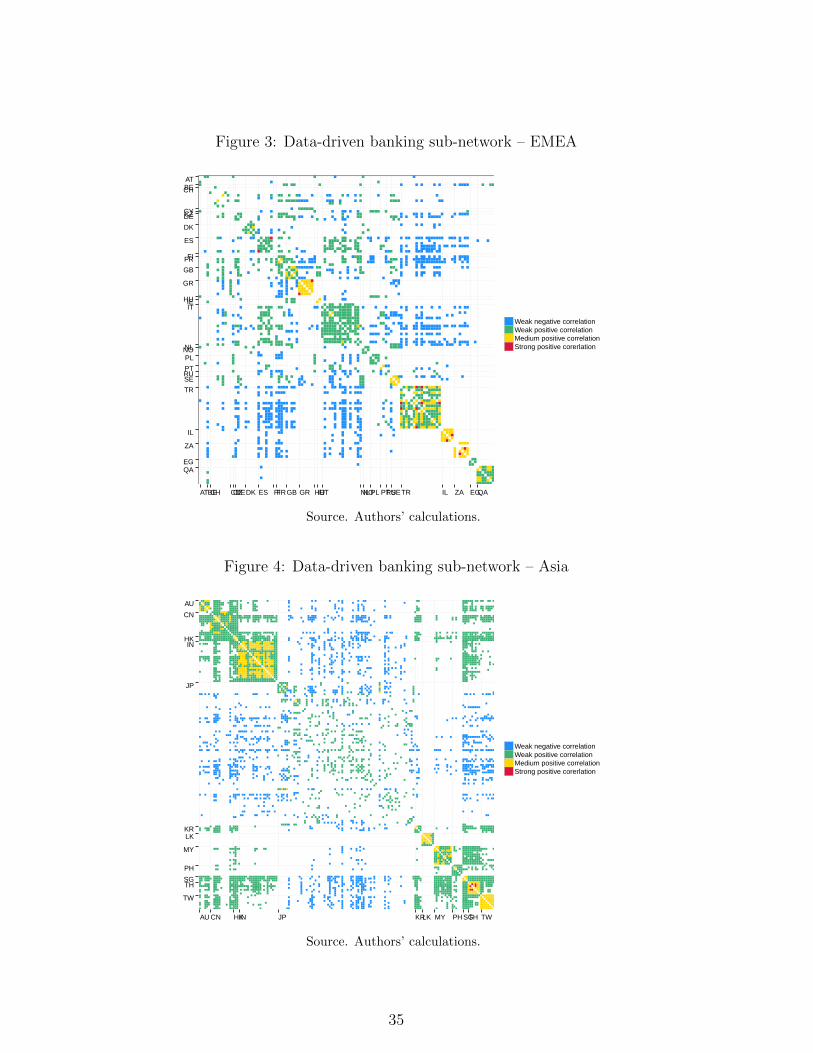
Figure 3: Data-driven banking sub-network – EMEA

ATBECH

CYCZDE

DK

ES

FIFR

GB

GR

HUIEIT

NLNOPL

PTRUSE

TR

IL

ZA

EGQA

ATBECH CYCZDEDK ES FIFRGB GR HUIEIT NLNOPL PTRUSETR IL ZA EGQA



Figure 4: Data-driven banking sub-network – Asia

AU

CN

HKIN

JP

KRLK

MY

PH

SGTH

TW

AU CN HKIN JP KRLK MY PHSGTH TW



35

Figure 5: Data-driven banking sub-network – Americas

AR

BR

CL

COPEMXCA

US

AR BR CL COPEMXCA US

Weak negative correlationWeak positive correlationMedium positive correlation


Figure 6: Data-driven banking sub-network – Cross-regional relationships

EMEA

Asia

Americas

EMEA Asia Americas



36

Figure 7: Data-driven banking sub-network – Cross-country relationships

EMEA

Asia

Americas

EMEA Asia Americas



Figure 8: Network model of tieringNetwork model of tiering

• A network exhibiting tiering should have this block-model form:

• Special kind of core-periphery model: emphasis on relation between core and periphery

• Tight on core, lax on periphery, makes sense for interbank market.


37

Figure 9: Network model of tiering - No penalty in PPInternational model of tiering

• A network exhibiting tiering should have this block-model form:

• If the ones in the periphery are due to regional factors, then these connections should not be penalized in the PP portion.


Figure 10: Core-periphery structure

Core

EMEA

Asia

Americas

Core EMEA Asia Americas


Source. Authors’ calculations. Original definition of the core as in Craig and von Peter (2014).

38

Figure 11: Core-periphery structure - Cross-country adjustment

Core

EMEA

Asia

Americas



Source. Authors’ calculations. Core definition allows intra-country links to be part of the periphery.

Figure 12: Core-periphery structure - Cross-region adjustment

Core

EMEA

Asia

Americas



Source. Authors’ calculations. Core definition allows intra-region links to be part of the periphery.

39

Figure 13: Random Matrices Eigenvalues

1.8 2 2.2 2.4 2.6 2.8 30

1

2

3

4

5

6

7

8

maximum eigenvalue

dens

ity


40

A. Sample of banks

Table A.1. Banks List

AT Erste Group Bank FR Natixis NO DNB ASA

Oberbank GB Alliance & Leicester SpareBank 1 SMN

Raiffeisen Bank International Barclays SpareBank 1 SR-Bank

BE Dexia Bradford & Bingley PL ING Bank Slaski

Fortis HBOS Bank Millennium

KBC HSBC Bank Pekao

CH Bank Coop Lloyds Banking Group PKO Bank Polski

Banque Cantonale Vaudoise Northern Rock PT Banco Comercial Portugues

Basler Kantonalbank Royal Bank of Scotland Banco Esprito Santo

Credit Suisse Standard Chartered BPI

EFG International GR Alpha Bank RU Sberbank

UBS National Bank of Greece VTB Bank

Valiant Eurobank Ergasias SE Nordea Bank

Vontobel Holding Attica Bank Skandinaviska Enskilda Banken

CY Hellenic Bank Public Bank of Greece Svenska Handelsbanken

CZ Komercni banka Piraeus Bank Swedbank

DE Commerzbank HU OTP Bank TR Akbank

Deutsche Bank IE Allied Irish Banks Albaraka Turk Katilim Bankasi

Deutsche Postbank Anglo Irish Bank Alternatifbank

Hypo Real Estate Bank of Ireland Asya Katilim Bankasi

Unicredit IT Banco di Desio e della Brianza DenizBank

IKB Banca Monte dei Paschi di Siena Finansbank

DK Danske Bank Banco Popolare Garanti Bank

Jyske Bank BP dell’Emilia Romagna Halk Bankasi

Spar Nord Bank Banca Popolare di Sondrio Turkiye Is Bankasi

Sydbank Capitalia Turkiye Kalkinma Bankasi

Vestjysk Bank Credito Bergamasco Sekerbank

ES BBVA Credito Emiliano Turk Ekonomi Bankasi

Bankinter Banca Carige Tekstilbank

Banco de Valencia Credito Valtellinese TSKB

Caixabank Intesa Sanpaolo VakifBank

Banco Pastor Mediobanca Yapi Kredi

Banco Popular Espanol Banca Etruria IL Israel Discount Bank

Banco de Sabadell Banca Popolare di Milano First International Bank of Israel

Santander Banca Profilo Bank Leumi Le-Israel

FI Aktia Bank Sanpaolo Imi Mizrahi Tefahot Bank

Pohjola Bank UBI Banca Bank Hapoalim

FR Credit Agricole Unicredit ZA Barclays Africa Group

BNP Paribas NL ING Group Capitec Bank

Societe Generale SNS Reaal FirstRand41

Table A.1. Banks List (continued)

ZA Nedbank IN Canara Bank JP Toho Bank Ltd

RMB Central Bank of India Tohoku Bank Ltd

Standard Bank Group Corporation Bank Michinoku Bank Ltd

EG Abu Dhabi Islamic Bank/Egypt Federal Bank Ltd Fukuoka Financial Group Inc

Suez Canal Bank Hdfc Bank Limited Shizuoka Bank Ltd

Commercial International Bank ICICI Bank Juroku Bank Ltd

QA Commercial Bank of Qatar Qsc Idbi Bank Ltd Suruga Bank Ltd

Doha Bank Qsc Indusind Bank Ltd Hachijuni Bank Ltd

Al Khaliji Bank Indian Overseas Bank Yamanashi Chuo Bank Ltd

Masraf Al Rayan Jammu and Kashmir Bank Ogaki Kyoritsu Bank Ltd

Qatar Islamic Bank Oriental Bank of Commerce Fukui Bank Ltd

Qatar International Islamic Punjab National Bank Hokkoku Bank Ltd

Qatar National Bank State Bank of India Shimizu Bank Ltd

AU ANZ Banking Group Syndicate Bank Shiga Bank Ltd

Bendigo And Adelaide Bank Uco Bank Nanto Bank Ltd

Bank of Queensland Union Bank of India Hyakugo Bank Ltd

Commonwealth Bank of Austral Ing Vysya Bank Ltd Bank of Kyoto Ltd

National Australia Bank Yes Bank Ltd Mie Bank Ltd

Westpac Banking Corp JP Shinsei Bank Ltd Hokuhoku Financial Group Inc

CN Ping An Bank Aozora Bank Ltd Hiroshima Bank Ltd

Bank of Ningbo Co Ltd -A Mitsubishi Ufj Financial Gro San-In Godo Bank Ltd

ICBC Resona Holdings Inc Chugoku Bank Ltd

Bank of Communications Co-H Sumitomo Mitsui Trust Holdin Tottori Bank Ltd

China Merchants Bank-H Sumitomo Mitsui Financial Gr Iyo Bank Ltd

Bank of China Ltd-H Daishi Bank Ltd Hyakujushi Bank Ltd

Huaxia Bank Co Ltd-A Hokuetsu Bank Ltd Shikoku Bank Ltd

China Minsheng Banking-A Nishi-Nippon City Bank Ltd Awa Bank Ltd

Bank of Nanjing Co Ltd -A Chiba Bank Ltd Kagoshima Bank Ltd

Industrial Bank Co Ltd -A Bank of Yokohama Ltd Oita Bank Ltd

Bank of Beijing Co Ltd -A Joyo Bank Ltd Miyazaki Bank Ltd

China Construction Bank-H Gunma Bank Ltd Higo Bank Ltd

China Citic Bank Corp Ltd-H Musashino Bank Ltd Bank of Saga Ltd

HK Hang Seng Bank Ltd Chiba Kogyo Bank Ltd Eighteenth Bank Ltd

Bank of East Asia Tsukuba Bank Ltd Bank of Okinawa Ltd

Boc Hong Kong Holdings Ltd Tokyo Tomin Bank Ltd Bank of The Ryukyus Ltd

Wing Hang Bank Ltd 77 Bank Ltd Yachiyo Bank Ltd

IN Allahabad Bank Aomori Bank Ltd Seven Bank Ltd

Axis Bank Ltd Akita Bank Ltd Mizuho Financial Group Inc

Bank of Baroda Yamagata Bank Ltd Kiyo Holdings Inc

Bank of India Bank of Iwate Ltd Yamaguchi Financial Group In

42

Table A.1. Banks List (continued)

JP Nagano Bank Ltd MY Rhb Capital Bhd CL Sm-Chile Sa-B

Bank of Nagoya Ltd PH Bdo Unibank Inc CO Bancolombia Sa

Aichi Bank Ltd Bank of The Philippine Islan Banco De Bogota

Daisan Bank Ltd Metropolitan Bank & Trust PE Bbva Banco Continental Sa-Co

Chukyo Bank Ltd Philippine National Bank MX Grupo Financiero Inbursa-O

Higashi-Nippon Bank Ltd Security Bank Corp Grupo Financiero Banorte-O

Taiko Bank Ltd Union Bank of Philippines CA Bank of Montreal

Ehime Bank Ltd SG Dbs Group Holdings Ltd Bank of Nova Scotia

Tomato Bank Ltd Oversea-Chinese Banking Corp Can Imperial Bk of Commerce

Minato Bank Ltd United Overseas Bank Ltd Canadian Western Bank

Keiyo Bank Ltd TH Bank of Ayudhya Pcl Home Capital Group Inc

Kansai Urban Banking Corp Bangkok Bank Public Co Ltd Laurentian Bank of Canada

Tochigi Bank Ltd Kasikornbank Pcl Genworth Mi Canada Inc

Kita-Nippon Bank Ltd Krung Thai Bank Pub Co Ltd National Bank of Canada

Towa Bank Ltd Siam Commercial Bank Pub Co Royal Bank of Canada

Fukushima Bank Ltd Thanachart Capital Pcl Toronto-Dominion Bank

Daito Bank Ltd Tmb Bank Pcl US Bear Stearns Cos Llc

Nomura Holdings Inc TW Chang Hwa Commercial Bank Associated Banc-Corp

KR Jeonbuk Bank Hua Nan Financial Holdings C American Express Co

Industrial Bank of Korea E.Sun Financial Holding Co Bank of America Corp

Woori Finance Holdings Co Mega Financial Holding Co Lt BB&T Corp

Shinhan Financial Group Ltd Taishin Financial Holding Bank of New York Mellon Corp

Hana Financial Group Sinopac Financial Holdings Bank of Hawaii Corp

Kb Financial Group Inc Ctbc Financial Holding Co Lt Bok Financial Corporation

LK Commercial Bank of Ceylon Pl First Financial Holding Boston Private Finl Holding

Dfcc Bank AR Banco Hipotecario Sa-D Shs Brookline Bancorp Inc

Hatton National Bank Plc Banco Macro Sa-B Bancorpsouth Inc

National Development Bank Pl Bbva Banco Frances Sa Citigroup Inc

Nations Trust Bank Plc Grupo Financiero Galicia-B Cathay General Bancorp

Sampath Bank Plc BR Banco ABC Brasil Commerce Bancshares Inc

Seylan Bank Plc Banco do Brasil Community Bank System Inc

MY Alliance Financial Group Bhd Banco Bradesco Cullen/Frost Bankers Inc

Affin Holdings Berhad Banco Panamericano City Holding Co

Ammb Holdings Bhd Banrisul Comerica Inc

Bimb Holdings Bhd Itau Unibanco Holding Sa Capital One Financial Corp

Cimb Group Holdings Bhd CL Banco De Credito E Inversion Columbia Banking System Inc

Hong Leong Bank Berhad Banco Santander Chile Cvb Financial Corp

Hong Leong Financial Group Banco De Chile City National Corp

Malayan Banking Bhd Corpbanca East West Bancorp Inc

Public Bank Berhad A.F.P. Provida S.A. First Commonwealth Finl Corp

43

Table A.1. Banks List (concluded)

US First Financial Bancorp US Susquehanna Bancshares Inc

First Finl Bankshares Inc Tcf Financial Corp

First Horizon National Corp Texas Capital Bancshares Inc

Fifth Third Bancorp Tfs Financial Corp

First Midwest Bancorp Inc/Il Trustmark Corp

Firstmerit Corp United Bankshares Inc

Fnb Corp Umb Financial Corp

First Niagara Financial Grp Umpqua Holdings Corp

Fulton Financial Corp Us Bancorp

Glacier Bancorp Inc Valley National Bancorp

Goldman Sachs Group Inc Westamerica Bancorporation

Huntington Bancshares Inc Washington Federal Inc

Hancock Holding Co Washington Mutual Inc

Hudson City Bancorp Inc Wachovia Corp

Iberiabank Corp Webster Financial Corp

JPMorgan Chase Wells Fargo

Keycorp Wintrust Financial Corp

Lehman Brothers Holdings Inc Zions Bancorporation

Mb Financial Inc

Mellon Financial Corp

Morgan Stanley

M&T Bank Corp

National City Corp

Natl Penn Bcshs Inc

Northern Trust Corp

New York Community Bancorp

Pacwest Bancorp

People’s United Financial

Provident Financial Services

Pnc Financial Services Group

Pinnacle Financial Partners

Park National Corp

Privatebancorp Inc

Regions Financial Corp

Signature Bank

Svb Financial Group

Synovus Financial Corp

S&T Bancorp

Suntrust Banks Inc

State Street Corp

Source. Bloomberg, The Banker.

44

working paper 16 27 - federal reserve bank of cleveland

Documents