working paper 437 september 2016 - center for global ... · pdf filepolicies are increasingly...
TRANSCRIPT

Working Paper 437September 2016
Results Through Transparency: Does
Publicity Lead to Better Procurement?
Abstract
Governments buy about $9 trillion worth of goods and services a year, and their procurement policies are increasingly subject to international standards and institutional regulation including the WTO Plurilateral Agreement on Government Procurement, Open Government Partnership commitments and International Financial Institution procurement rules. These standards focus on transparency and open competition as key tools to improve outcomes. While there is some evidence on the impact of competition on prices in government procurement, there is less on the impact of specific procurement rules including transparency on competition or procurement outcomes. Using a database of World Bank financed contracts, we explore the impact of a relatively minor procurement rule governing advertising on competition using regression discontinuity design and matching methods. The rule does appear to have a small, positive impact on bidding levels, suggesting the potential for more significant and strongly enforced transparency initiatives to have a sizeable effect on procurement outcomes..
JEL Codes: H57, D40, D73
Keywords: procurement, advertising, transparency, competition
www.cgdev.org
Charles Kenny and Ben Crisman
Center for Global Development2055 L Street NW
Washington, DC 20036
202.416.4000(f) 202.416.4050
www.cgdev.org
Results Through Transparency: Does Publicity Lead to Better Procurement?
Charles KennyCenter for Global Development
Ben CrismanCenter for Global Development
The authors thank Justin Sandefur for econometric advice and guidance and colleagues at CGD for valuable feedback during a presentation of early results.
The Center for Global Development is grateful for contributions from the Omidyar Network and the UK Department for International Development in support of this work.
Charles Kenny and Ben Crisman. 2016. "Results Through Transparency: Does Publicity Lead to Better Procurement?." CGD Working Paper 437. Washington, DC: Center for Global Development.http://www.cgdev.org/publication/results-through-transparency-does-publicity-lead-better-procurement-working-paper-437
The Center for Global Development is an independent, nonprofit policy research organization dedicated to reducing global poverty and inequality and to making globalization work for the poor. Use and dissemination of this Working Paper is encouraged; however, reproduced copies may not be used for commercial purposes. Further usage is permitted under the terms of the Creative Commons License.
The views expressed in CGD Working Papers are those of the authors and should not be attributed to the board of directors or funders of the Center for Global Development.
Table of Contents
Introduction 3
Literature Review 5
Data Overview 6
Econometric Strategy 11
Regression Discontinuity Design . . . . . . . . . . . . . . . . . . . . . . . . . . . . . 11
Matching Methods . . . . . . . . . . . . . . . . . . . . . . . . . . . . . . . . . . . . 15
Empirical Results 17
Regression Discontinuity Estimates . . . . . . . . . . . . . . . . . . . . . . . . . . . 20
Matching Estimates . . . . . . . . . . . . . . . . . . . . . . . . . . . . . . . . . . . 24
Conclusion 25
2

IntroductionCurrent estimates place the size of government contracting at $9,000,000,000,000 per year
globally (Kenny and Karver, 2012). This procurement is governed by rules on tender prepa-
ration, advertising, bidding procedures and selection methods that vary between countries,
institutions, and tender types. The stated aim of most rules is to ensure value for money
delivering a high quality product at the lowest price. An intermediate aim for many tenders
is to maximize competition as a tool to deliver that result. The presence of numerous bidders
is at least one indication of active competition for contracts. It may reflect a strong and clear
set of bid documents, a clear and simple bid process, the perception of a level playing field
for bidders, and a client with the capacity and incentives to treat winning contractors fairly.1
Procurement rules are frequently designed to maximize competition through creating a
(perceived) level playing field, standardizing processes and advertising bid opportunities. A
number of transparency initiatives including the Open Contracting Partnership seek to foster
the level playing field and awareness in the procurement process through publication and
data release.2 While we will see there is some nascent evidence that these approaches work,
the empirical case for the impact of transparency on procurement is still partial at best. This
paper seeks to add to the evidence base, using World Bank financed contracts as the subject
of analysis.
The World Bank finances approximately 20 billion USD in government contracting
each year.3 Bank-financed goods, works, and services are usually procured following a set
of guidelines published by the institution. The guidelines outline a number of different
procurement approaches applicable to different goods and services –including commodified
low-cost goods, consultancies, and more complex construction, or services projects. Amongst
competitively bid works procurements, one variation of rules is between National Competitive
Bid (NCB) and International Competitive Bid (ICB). The difference between the two are
comparatively minor, involving the language of documents and the advertising of the tender
opportunity. According to the procurement guidelines, NCB:
May be the most appropriate way of procuring goods or works which, by their
nature or scope, are unlikely to attract foreign competition. . . Advertising may
1At the same time we should note there is a significant difference between the number of bidders and thelevel of ‘actual’ competition in practice, especially in cases where a number of the bidders are colluding orsubmit frivolous or very weak bids. This has been found to be a common problem in the case of a sample ofWorld-Bank financed infrastructure bids in Africa, for example (Africon, 2008).
2See http://www.open-contracting.org/3http://go.worldbank.org/GM7GBOVGS0
3

be limited to the national press or official gazette, or a free and open access
website. Bidding documents may be only in a national language of the borrower’s
country. . . If foreign firms wish to participate under these circumstances, they
shall be allowed to do so.4
According to the procurement guidelines for ICB:
The Bank will arrange for. . . publication in UN Development Business online
(UNDB online) Prequalification and bidding documents and the bids shall be
prepared in one of . . . English, French, or Spanish. . . . Bidding documents shall
be so worded as to permit and encourage international competition.
ICB is designed to increase competition and attract leading international firms to work on
large, complex contracts. As such, it is linked to some of the oldest justifications for donor
involvement in investment lending –that client countries lack the hard currency and the
technical capacity to deliver complex development projects and require foreign exchange and
foreign expertise to compensate for these shortcomings. At the same time, the practical
difference between the approaches is limited –NCB is open to international bidders, for
example, and ICB is open to nationals. (Indeed, as a practical matter, nationals usually win
ICBs; looking at our dataset of World Bank financed goods and works contracts awarded
between 1995 and 2007, local firms have accounted for 70.38 percent of the value of ICB
contracts.)
Given the practical difference between NCB and ICB procurements is limited to advertising
and language, any difference in outcomes between ICB and NCB might be taken as a measure
of the impact of advertising and language. We will see the picture is not that simple, however:
ICB and NCB approaches are selected in part based on the nature of the goods and works
being contracted –including if they are likely to appeal to international bidders.
In an attempt to overcome this problem and measure the ‘true’ impact of transparency
we use a fuzzy regression discontinuity design that exploits the fact that the World Bank
sets thresholds on the size of contracts that mandates the use of ICB. Contracts just smaller
than the threshold are unlikely to be markedly different than contracts just larger than the
threshold, and so any difference in observed competition outcomes can more fairly be said
to reflect the impact of moving from NCB to ICB rules. While our regression discontinuity
design does present some evidence for a positive impact on bidding outcomes from ICB, our
4http://siteresources.worldbank.org/INTPROCUREMENT/Resources/ProcGuid-10-06-RevMay10-ev2.pdf
4
estimates suffer from what can be described as a weak instrument problem –for this reason
we also employ two matching techniques which similarly describe a positive impact of ICB
on bidding outcomes, though of lessened magnitude.
The outcomes we consider include the total number of bidders a contract receives, the
nationality of bidders, the number of addenda, and days to contract finalization. Both our
regression discontinuity design and matching techniques identify an increase in the number
of bidders and in ex-post renegotiation as a result of increased publicity. We find mixed
evidence on the effects of ICB on the nationality of bidders, however, the weight of the
evidence suggests that listing a contract through International Competitive Bidding results
in an increase in foreign bidders overall and an increase in bidders from OECD countries.
Unfortunately, we have no way of directly estimating price effects, though we offer some
suggestive evidence that prices were largely unaffected by ICB status.
Literature ReviewIt is a common argument that competition improves outcomes (Smith, 1776). There is
evidence that this applies to government procurement. Iimi (2006) finds that the winning
bid on Japanese aid projects falls as a proportion of the ex-ante cost estimate as the number
of bidders climbs to eight. Estache and Iimi (2008) suggest that improved competition on
developing country infrastructure projects would reduce prices by an average of 8 percent
with the effect reaching its maximum between 4 and 14 bids. Onur et al. (2012) finds that
competition reduces price of Turkish public procurements as does allowing foreign bidders.
Galletta et al. (2015) suggest DRC roads contract prices are lower where there are more
bidders.
There is also evidence that the form of procurement process as well as the environment
in which the procurement takes place can impact levels of competition and pricing. Ohashi
(2009) suggests that removing discretion on bidder qualification reduces prices by 3 percent
in Japanese local contracting. Soraya (2009) finds transparency in a World Bank Urban
Infrastructure Project in Bali may have generated prices that were lower by 21 percent while
Kenny (2010) finds World Bank Financed road construction costs are lower where measures
of Voice and Accountability are high.
Specifically regarding tender advertising and transparency, Pavel et al. (2013) look at
contracting in the Slovak Republic and find that e-procurement and advertising leads to
more bids and lower prices. And in perhaps the closest analysis to the one we will perform in
5
this paper, Coviello and Mariniello (2014) use regression discontinuity to suggest advertising
Italian local government tenders at the regional level increases bidders and reduces prices.
This paper uses a database of over 65,000 World Bank works contracts to look at specific
procurement rule around advertising/language, employing a regression discontinuity approach
in an attempt to find a causal link. We also look at the impact of procurement rules on the
participation of foreign bidders in particular as one of the primary reasons for employing ICB
is to attract such bidders. The discontinuity we exploit is that the World Bank mandates the
use of ICB on contracts over a threshold estimated contract size set at the country level. Many
ICBs involve contracts that are significantly below that threshold, but the threshold still
appears to act as a forcing mechanism for enough contracts that we can use that discontinuity
to evaluate the impact of moving from NCB to ICB.
As well as measuring the impact of transparency, this paper will provide some evidence
about the widespread assumption that ‘strong procurements’ –well designed, well managed bid
documents that attract high bidder interest– are associated with ‘strong agencies’ or ‘strong
institutional environments’ for procurement. This is linked to an assumption that country-
level characteristics are responsible for a substantial part of the variability in procurement
indicators. Not least, country-level procurement assessments based on this assumption feed
into World Bank Country Policy and Institutional Analysis rankings that in turn help to
determine allocations from the Bank’s soft lending arm, IDA. Similarly, at the agency level,
the focus on agency capacity in procurement risk assessments as part of World Bank project
appraisal, for example. This stands in contrast to Estache and Iimi (2008), who specify a
bid model in terms of particular technical details of a contract, suggesting it is such details
that predominate in determining procurement outcomes. The analysis should provide some
indication of whether ‘strong procurements’ as measured by competition as well as negotiation
time and number of amendments are largely the result of ‘strong agencies,’ ‘strong countries’
or contract idiosyncrasies.
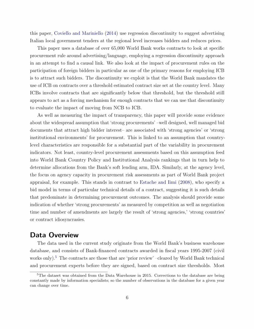
Data OverviewThe data used in the current study originate from the World Bank’s business warehouse
database, and consists of Bank-financed contracts awarded in fiscal years 1995-2007 (civil
works only).5 The contracts are those that are ‘prior review’ –cleared by World Bank technical
and procurement experts before they are signed, based on contract size thresholds. Most
5The dataset was obtained from the Data Warehouse in 2015. Corrections to the database are beingconstantly made by information specialists; so the number of observations in the database for a given yearcan change over time.
6
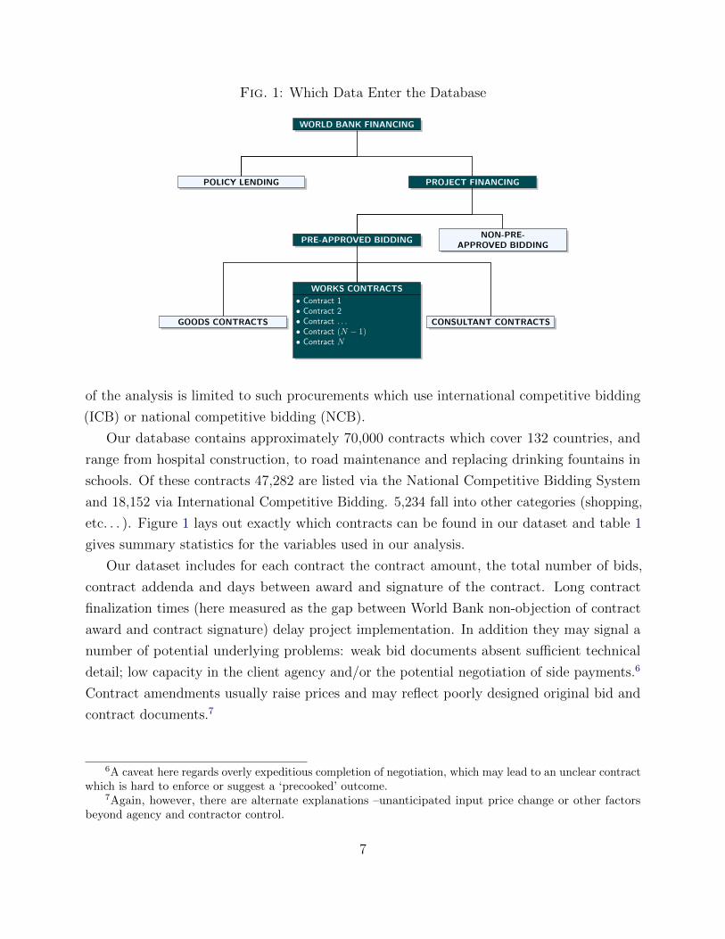
Fig. 1: Which Data Enter the Database
WORLD BANK FINANCING
POLICY LENDING PROJECT FINANCING
PRE-APPROVED BIDDINGNON-PRE-
APPROVED BIDDING
GOODS CONTRACTS CONSULTANT CONTRACTS
WORKS CONTRACTS
• Contract 1• Contract 2• Contract . . .• Contract (N − 1)• Contract N
of the analysis is limited to such procurements which use international competitive bidding
(ICB) or national competitive bidding (NCB).
Our database contains approximately 70,000 contracts which cover 132 countries, and
range from hospital construction, to road maintenance and replacing drinking fountains in
schools. Of these contracts 47,282 are listed via the National Competitive Bidding System
and 18,152 via International Competitive Bidding. 5,234 fall into other categories (shopping,
etc. . . ). Figure 1 lays out exactly which contracts can be found in our dataset and table 1
gives summary statistics for the variables used in our analysis.
Our dataset includes for each contract the contract amount, the total number of bids,
contract addenda and days between award and signature of the contract. Long contract
finalization times (here measured as the gap between World Bank non-objection of contract
award and contract signature) delay project implementation. In addition they may signal a
number of potential underlying problems: weak bid documents absent sufficient technical
detail; low capacity in the client agency and/or the potential negotiation of side payments.6
Contract amendments usually raise prices and may reflect poorly designed original bid and
contract documents.7
6A caveat here regards overly expeditious completion of negotiation, which may lead to an unclear contractwhich is hard to enforce or suggest a ‘precooked’ outcome.
7Again, however, there are alternate explanations –unanticipated input price change or other factorsbeyond agency and contractor control.
7

Table 1: Summary Statistics
Variable Mean Std. Dev. Min. Max. N
ICB 0.281 0.45 0 1 65,794No. Bids Received 5.99 22.99 0 824 71,028Foreign Bids 0.28 0.70 0 4 71,028OECD Bids 0.19 0.70 0 4 71,028Chinese Bids 0.21 0.79 0 4 71,028No. of Addenda 0.27 0.77 0 22 71,028Days to Finalization 44.42 79.70 0 2074 65,845
Value of Contract 1.03 4.90 0 446.62 71,028(in millions)School Contract 0.08 0.26 0 1 71,028Road Contract 0.16 0.37 0 1 71,028Construction Contract 0.31 0.461 0 1 71,028Hospital Contract 0.02 0.13 0 1 71,028Agency Experience 492.30 699.40 1 2885 71,028
In addition, we have data on the country of origin of bidders, as well as country and
agency issuing the contract. We use the agency data to construct a proxy for procurement
experience, simply using the number of times a particular agency is listed as the implementor
throughout the database. We also identify particular kinds of projects by their title, identifying
contracts whose title includes “constru,8” “road,” “hospital,” or “school.” Contracts are
further categorized by type (Maintenance, Infrastructure, Civil Works, Buildings) and sector
(Transportation, Sanitation, Agriculture, etc.). Taking data available from World Bank
documentation we construct a set of thresholds that mandate the use of ICB for contracts
over a given size in particular countries. A full tabulation of these variables can be found in
the appendix.
There are a number of caveats about data quality. First, the number of bidders is not
validated by World Bank staff, and practices on what is entered may vary (bid documents
purchased versus bids received versus bids evaluated, for example). There are a number of
extreme (and repeated) outliers in the number of bidders which received 800+ bids which
we take to be suggestive of coding error rather than overwhelming competition. For this
reason we censor our bids received variable at 100 bids. Similarly we only have the country of
origin for up to four bidders. Consequently our number of foreign bidders variable is heavily
censored at 4. Data on bidder country origin is based on country of registration –so that
local subsidiaries of international firms will be reported as national firms. Agency names
8For construction we require the string to include ‘constru’ rather than construction to avoid a number ofspelling errors and abbreviations.
8

are not standardized, suggesting that contracts issued by one agency may be listed under
two different agencies. This will add noise to the agency experience variable. Regarding the
thresholds data, there is a concern that given the approval dates for the contracts in this
dataset range from 1995 to 2007, the thresholds or procurement methods almost certainly
have changed over time.9 Certain projects will set their own ICB threshold levels which
might be lower than a country’s national threshold. However, use of these thresholds would
introduce substantial endogeneity issues. This and other data entry errors will at the least
add noise and may add unobserved bias. Given the (still) comparatively large sample size
of well-documented contracts, it is still to be hoped that these errors are comparatively
unimportant in terms of biasing results.
Additionally, the contract value data we have are for realized contract value, or the actual
value of the contract that was financed. The decision to mandate listing as ICB is made
based on the engineer’s estimate of what the (package of) contract(s) should cost, ex-ante.
Thus, if ICB “works” and reduces the price of an project, it could reduce it to below the
value of a similar NCB contract.10 We will discuss these and our econometric solutions to
these problems in more detail in section .
The data allows us to illustrate a number of interesting trends and country statistics
regarding World Bank financed works contracts. Looking at out three procurement measures
we find that:
1. On average ICB contracts are more likely to have a high number of bidders compared to
NCB and other procurement methodologies. As can be seen in Table 2, 77.3 percent of
9We have requested these historical thresholds data from the World Bank Feb. 29 2016 and are awaitinga response.
10An additional issue is that under World Bank procurement guidelines, similar, but discrete contractscan be listed together to allow large companies to bid for all of them at once. Paragraph 2.4 of Guidelines:Procurement under IBRD Loans and IDA Credits (2004) states the following: “For a project requiringsimilar but separate items of equipment or works, bids may be invited under alternative contract optionsthat would attract the interest of both small and large firms, which could be allowed, at their option, to bidfor individual contracts (slices) or for a group of similar contracts (package). All bids and combinations ofbids shall be received by the same deadline and opened and evaluated simultaneously so as to determinethe bid or combination of bids offering the lowest evaluated cost to the Borrower.” This means that theex-post contract values that we have may represent a fractional component of the engineer’s estimate. Forexample, a school building contract in Afghanistan listed under X-project requests a number of schools withthe same specifications in different areas. The actual value of each of these ICB listed works contracts isaround 500,000USD, well under the 5,000,000USD threshold for ICB procurement. Combined, they equalapproximately 12,000,000USD over the threshold. While there is no way to tell with certainty whether eachof these contracts was listed via this alternative contracts method, it would be less likely that X local schoolconstruction contracts would be listed through the ICB system were it not that the combined contract valuesurpassed the country threshold.
9
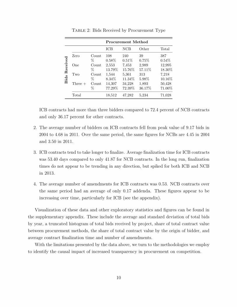
Table 2: Bids Received by Procurement Type
Procurement Method
ICB NCB Other Total
BidsReceived Zero Count 108 240 39 387
% 0.58% 0.51% 0.75% 0.54%One Count 2,553 7,453 2,989 12,995
% 13.79% 15.76% 57.11% 18.30%Two Count 1,544 5,361 313 7,218
% 8.34% 11.34% 5.98% 10.16%Three + Count 14,307 34,228 1,893 50,428
% 77.29% 72.39% 36.17% 71.00%
Total 18,512 47,282 5,234 71,028
ICB contracts had more than three bidders compared to 72.4 percent of NCB contracts
and only 36.17 percent for other contracts.
2. The average number of bidders on ICB contracts fell from peak value of 9.17 bids in
2004 to 4.68 in 2011. Over the same period, the same figures for NCBs are 4.45 in 2004
and 3.50 in 2011.
3. ICB contracts tend to take longer to finalize. Average finalization time for ICB contracts
was 53.40 days compared to only 41.87 for NCB contracts. In the long run, finalization
times do not appear to be trending in any direction, but spiked for both ICB and NCB
in 2013.
4. The average number of amendments for ICB contracts was 0.53. NCB contracts over
the same period had an average of only 0.17 addenda. These figures appear to be
increasing over time, particularly for ICB (see the appendix).
Visualization of these data and other exploratory statistics and figures can be found in
the supplementary appendix. These include the average and standard deviation of total bids
by year, a truncated histogram of total bids received by project, share of total contract value
between procurement methods, the share of total contract value by the origin of bidder, and
average contract finalization time and number of amendments.
With the limitations presented by the data above, we turn to the methodologies we employ
to identify the causal impact of increased transparency in procurement on competition.
10
Econometric StrategyOur primary aim is to estimate the effect of an increase in publicity mandated for World
Bank financed ICB contracts (as compared to NCB contracts) on measures of competition
as proxied by the number of bids a contract receives. To do this we estimate the following
equation:
Yi = α + βICB + γXi + θc + λt + ψs + εi (1)
Where Yi is the procurement outcome of interest, here number of bids received, type of bids
received, the number of addenda and time to contract finalization, for contract i; Xi is a
vector of contract characteristics including the log value of the contract, implementing agency
experience, the number of contracts in a project, and other contract characteristics; θc, λt, ψs
are, respectively, country, type (Maintenance, Infrastructure, Civil Works, Buildings) and
sector (Transportation, Sanitation, Agriculture, etc.) fixed effects for country c, type t, and
sector s; and ICB is an indicator variable for whether or not the contract was listed using
the ICB or NCB.
We begin by estimating a simple Ordinary Least Squares (OLS) regression. We estimate
the effects of being listed via the International Competitive Bidding system on procurement
outcomes (namely, number and qualities of bids) controlling for country and contract-level
characteristics. Due to characteristics of our dependent variables we also employ a negative-
binomial regression for total number of bids received (which displays negative binomial
distribution, see figure 7) and Tobit regressions for foreign, OECD, and China bidders as
they are heavily censored at four bids.11 For each of these regressions we calculate robust
standard errors.
Regression Discontinuity DesignWe are concerned that some unobservable characteristic(s) of contracts might cause
certain low-value contracts to be listed via ICB. For this reason, contracts with similar (low)
dollar values and similar control characteristics that only differ in method of listing and
thus seem comparable may be receiving different number of bids due to these unobservable
characteristics. The likely effect of this is indeterminate; it might induce a downward bias in
the estimated coefficient (because those contracts most likely to have fewest domestic bids
would be those listed through the international system), or it may bias estimates upward as
it may be that contracts most likely to attract foreign bids might be listed through ICB.
11Where Y ∗i is a latent variable for foreign/OECD/Chinese bids taking the form: Yi =
{4 if Y ∗
i > 4
Y ∗i if Y ∗
i ≤ 4
11
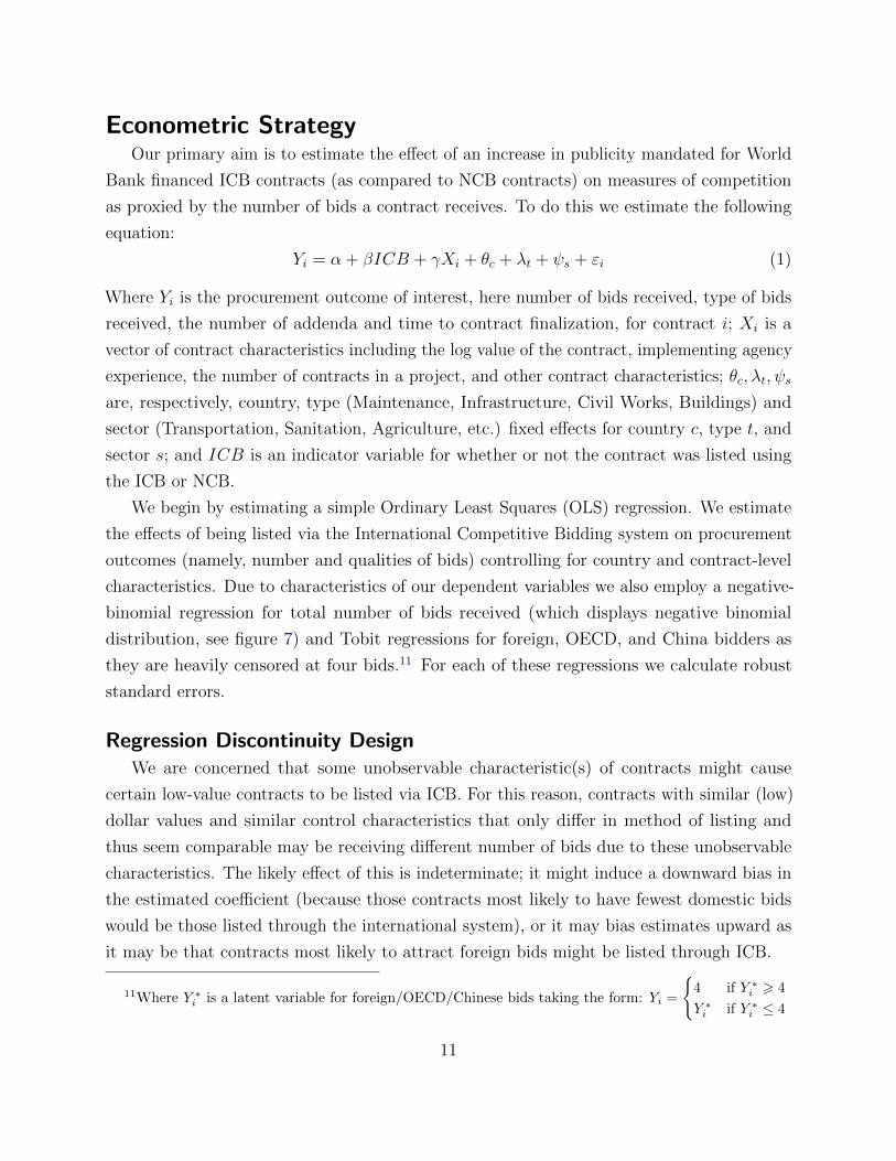
Fig. 2: Enforcement of Procurement Rules
Note: While World Bank procurement rules do allow for con-tracts lower than the threshold to be listed as ICB, we note thatthese distributions suggest that few observations are forced intobeing listed as ICB instead of NCB. Rather, we observe manyprocurement officers are self-selecting contracts into ICB.
For this reason, we attempt to employ a Regression Discontinuity Design (RDD) exploiting
the existence of a threshold value at which a contract is required to be listed via ICB. The
basic logic for the RDD is as follows; if procurement procedures are implemented and followed
as intended (with no manipulation), there should be no reason to believe that the average
contract with a value of one dollar less than the treatment (listing) determining threshold (T-
1) should be statistically different from the average contract immediately above the threshold
(T+1) except for the impact caused by the treatment (Lee and Lemieux, 2010). Thus, by
measuring the magnitude of the discontinuity immediately around the threshold, we should
be able to estimate the local average treatment effect (LATE) of increased advertising on bid
competition. We first estimate a sharp regression discontinuity design. We estimate local
linear regressions on either side of the cutoff, allowing the slope of the line to change either
side, as in equation 2:
Yi = β0 + β1Vic + τEi + β2Ei · Vic + εi (2)
This sharp RD estimates the Intention to Treat effect. As mentioned above, however, a valid
sharp RD would require that no contracts with a value above the threshold would be listed
via NCB (untreated) and no contracts with a value below the threshold would be listed via
ICB (treated) (Hahn et al., 2001). As can be seen in figure 2, this is not the case around our
12

threshold. We do see fairly consistent application of treatment to contracts which are above
the threshold –i.e. most of those who should be treated are treated. But there are many
contracts listed under the ICB system who have values far below the threshold. This likely
reflects a preference by the World Bank for financed contracts that could plausibly attract
international competition to be listed as ICB. However, given that there is still an observable
increase in the likelihood of being listed as ICB at the threshold (suggesting the cutoff still has
some independent influence to list as NCB or ICB), we are able to overcome this characteristic
by employing a Fuzzy Regression Discontinuity Design (FRDD) as presented in Lee and
Lemieux (2010).
We implement this approach using the 2SLS estimator as discussed in Hahn et al. (2001).
We first regress realized ICB (whether or not a contract was actually listed as ICB) against
an eligibility dummy, E. In the second stage, we estimate the impact of ICB on the outcome
variables using the value of ICB predicted in the first. In both stages, we include an
interaction terms between ICB/E and the logged value of the contract relative to country
threshold (denoted V ). This technique will estimate the effect of treatment on the treated
(ToT).
ICBi = α0 + α1Vic + πEi + α2Ei · Vic + µi (3)
Yi = β0 + β1Vic + τ ICBi + β2ICBi · Vic + εi (4)
Hahn et al. (2001) identify the key assumptions for the (F)RDD to be valid. First among
these is continuity in the running variable. If estimated contract values are being artificially
adjusted around the threshold so that the contract can be listed via NCB (or must be via
ICB), the regression discontinuity design would not be valid. Note we are using actual
contract values rather than estimates, which would blunt the impact of such manipulation.
Nonetheless, we can test for this assumption using the McCrary (2008) test. This test
determines if the density of the running variable experiences a discontinuous change at the
threshold, which, if it does, would suggest that individuals are purposefully altering estimated
contract values so that they will fall into either the treated or non-treated category.
We test the continuity in density of the running variables when transformed logarithmically.
We take the natural log of the value less the natural log of the country threshold, essentially
taking the natural log of the value of the contract relative to its country threshold. This
allows us to more consistently compare across countries while preserving a stable threshold
of zero when the contract value is equal to the threshold. When we run the McCrary test
with this transformation we observe a normal distribution of relative contract values with no
13

Fig. 3: Visualization of the McCrary Test
Note: Y-Axis is the density of observations. X-Axis is the runningvariable (log-centered value of the contract). Graphic constructedusing the -DCdensity- command in Stata.
observable or statistically significant change in density immediately around the threshold, see
figure 3. While we are unable to directly test price effects, this test also gives some indication
that there is no price effect.12
A final assumption in the validity of the Fuzzy Regression Discontinuity Design is that
there exists at the threshold a discontinuous jump in the likelihood of treatment. Figure 4
delineates the findings of the first stage of our FRDD estimator. At the bandwidth derived
using the Imbens and Kalyanaraman (2011) optimal bandwidth algorithm (bw = 2.94) we do
observe a small but significant jump in the likelihood of treatment. We observe the same
at twice this bandwidth, however, this jump loses significance at 50 percent of this optimal
bandwidth. The reason for this is likely stems from two data-related issues. First, while
contracts whose estimated value is above the threshold limit are required to be listed via
ICB the reverse is not true of those contracts with values below the threshold. As figure 4
makes clear, many contracts use ICB even below the required threshold value. Second, as
mentioned above, the data we have for the running variable and not the estimated value on
which the listing decision was made. There will be both positive and negative variation in
12For example, if the true value of the contract is equal to y∗, under NCB rules the price is simply y∗.However, if y∗ is greater than the threshold value c the probability of being listed as ICB should increase.Thus, assuming a smooth distribution of y∗, in the presence of a negative price effect (where the observedprice y < y∗) we should observe a decrease in the density of y immediately around the cut off. Therefore, wefind no evidence for a price effect, but neither should this be taken as rigorous evidence of a null effect.
14

Fig. 4: Discontinuity in the Probability of Being Listed as ICB
(A) 50% Bandwidth (B) 100% Bandwidth (C) 200% Bandwidth
Note: Local Linear Regressions over scatterplots of binned (rounded) values.
the difference between the actual and estimated costs. This uncertainty will likely reduce the
observed discontinuity in receiving treatment though the magnitude of this will depend on
the extent and average direction of this variation. We anticipate that if ICB works to reduce
the awarded price of a contract through increased competition, we should expect some ICB
contracts whose values were estimated immediately above the contract to appear in our data
just below the threshold. This reduction in size of the discontinuity will likely bias upwards
the final estimated LATE in that we underestimate the difference in the denominator of
the wald estimator. As this estimate approaches zero, the estimated LATE will increase
dramatically.
Matching MethodsAs we show in the preceding section, the discontinuous increase in the probability of being
listed as ICB is small and suffers from what can be considered a weak instrument problem.
For this reason, we also present the results of two matching techniques; traditional Nearest
Neighbor Propensity Score Matching (PSM), and Coarsened Exact Matching (CEM). In the
absence of randomization or the ‘as-if’ randomization induced via the regression discontinuity
design the researcher makes several assumptions to identify the treatment effect, τATT . The
true effect of treatment on the treated is characterized in equation 5; in essence, the difference
between an observation which has been treated and what that same observation would be in
the absence of treatment (Caliendo and Kopeinig, 2008).
τATT = E(τ |T = 1) = E[Y (1)|D = 1]E[Y (0)|D = 1] (5)
15

However, given that it is impossible for us to observe an individual contract’s outcome both
with and in the absence of treatment, matching techniques allow us to pair similar observations
from both treated and non-treated groups. As Rosenbaum and Rubin (1983) demonstrate,
it is possible to construct balancing scores from the propensity score, P (T = 1|X) = P (X).
A variety of algorithms allow us to match observations which hold a similar probability of
being selected into treatment based on relevant characteristics. From there we can estimate
the average treatment effect on the treated by comparing mean outcomes for both groups.
The estimator employed via the Propensity Score matching techniques can be generalized to
the following:
τPSMATT
= E(τ |T = 1) = E[Y (1)|D = 1]− E[Y (0)|D = 1] (6)
This methodology makes several assumptions to invoke a causal claim. First among this is that
there is no selection based on unobservables and that all values which do determine selection
can be observed (Y (0), Y (1)∐D|P (X),∀X). We concede that there are a number of reasons
why one might suspect that in this case selection on idiosyncratic contract unobservables
might play a role. However, we argue that as our regression discontinuity estimates, which will
not be responsive to this potential bias, similarly find a positive effect of ICB on bidding this is
of secondary concern. We match contracts on every contract characteristic that is unaffected
by treatment, including the natural log of the contracted amount, sector, type, year, country,
implementing agency experience, the number of contracts in a project (complexity), and
whether or not the contract name includes “constru,13”“road,” “hospital,” or “school.” The
second assumption is that of sufficient overlap in propensity scores between the treated and
non-treated groups. As can be seen in figure 5, there is substantial overlap in the propensity
score.
The third assumption14 demands an appropriate specification of the logit/probit model
used to estimate the propensity score. We estimate the propensity score with a number of
specifications, alternately excluding variables, and obtain qualitatively similar scores in each.
However, despite these efforts we are unable to completely reduce bias using these techniques.
This is likely due to the high-dimensionality of the data and overlapping contract level
characteristics which can be inversely correlated. For this reason we also employ Coarsened
Exact Matching (CEM) as presented in Iacus et al. (2011). CEM breaks variables into
appropriately sized categories on which it then performs an exact matching algorithm. This
13Several construction observations are abbreviated to “constru.” or include misspellings in the final fewcharacters.
14A fourth assumption requires stable unit treatment values, or that the outcome of one unit is not changedby the treatment status of others. We do not expect this dynamic here.
16
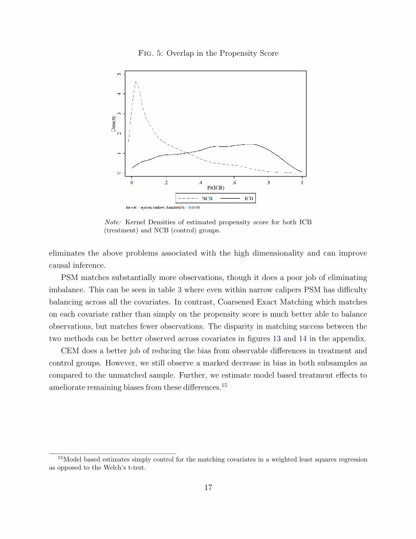
Fig. 5: Overlap in the Propensity Score
Note: Kernel Densities of estimated propensity score for both ICB(treatment) and NCB (control) groups.
eliminates the above problems associated with the high dimensionality and can improve causal inference.
PSM matches substantially more observations, though it does a poor job of eliminating imbalance. This can be seen in table 3 where even within narrow calipers PSM has difficulty balancing across all the covariates. In contrast, Coarsened Exact Matching which matches on each covariate rather than simply on the propensity score is much better able to balance observations, but matches fewer observations. The disparity in matching success between the two methods can be better observed across covariates in figures 13 and 14 in the appendix.
CEM does a better job of reducing the bias from observable differences in treatment and control groups. However, we still observe a marked decrease in bias in both subsamples as compared to the unmatched sample. Further, we estimate model based treatment effects to ameliorate remaining biases from these differences.15
15Model based estimates simply control for the matching covariates in a weighted least squares regressionas opposed to the Welch’s t-test.
17
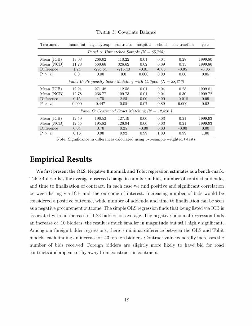
Table 3: Covariate Balance
Treatment lnamount agency exp contracts hospital school construction year
Panel A: Unmatched Sample (N = 65,785)
Mean (ICB) 13.03 266.02 110.22 0.01 0.04 0.28 1999.80Mean (NCB) 11.28 560.66 326.62 0.02 0.09 0.33 1999.86Difference 1.74 -294.64 -216.40 -0.01 -0.05 -0.05 -0.06P > |z| 0.0 0.00 0.0 0.000 0.00 0.00 0.05
Panel B: Propensity Score Matching with Calipers (N = 28,756)
Mean (ICB) 12.94 271.48 112.58 0.01 0.04 0.28 1999.81Mean (NCB) 12.78 266.77 109.73 0.01 0.04 0.30 1999.72Difference 0.15 4.75 2.85 0.00 0.00 -0.018 0.09P > |z| 0.000 0.447 0.05 0.07 0.89 0.000 0.02
Panel C: Coarsened Exact Matching (N = 12,526 )
Mean (ICB) 12.59 196.52 127.19 0.00 0.03 0.21 1999.93Mean (NCB) 12.55 195.82 126.94 0.00 0.03 0.21 1999.93Difference 0.04 0.70 0.25 -0.00 0.00 -0.00 0.00P > |z| 0.16 0.90 0.92 0.99 1.00 0.99 1.00
Note: Significance in differences calculated using two-sample weighted t-tests.
Empirical Results We first present the OLS, Negative Binomial, and Tobit regression estimates as a bench-mark. Table 4 describes the average observed change in number of bids, number of contract addenda, and time to finalization of contract. In each case we find positive and significant correlation between listing via ICB and the outcome of interest. Increasing number of bids would be considered a positive outcome, while number of addenda and time to finalization can be seen as a negative procurement outcome. The simple OLS regression finds that being listed via ICB is associated with an increase of 1.23 bidders on average. The negative binomial regression finds an increase of .10 bidders, the result is much smaller in magnitude but still highly significant. Among our foreign bidder regressions, there is minimal difference between the OLS and Tobit models, each finding an increase of .43 foreign bidders. Contract value generally increases the number of bids received. Foreign bidders are slightly more likely to have bid for road contracts and appear to shy away from construction contracts.
18
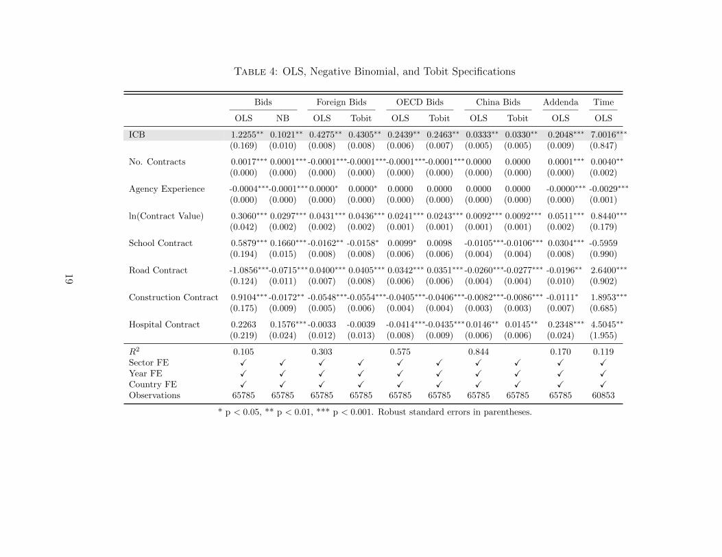
Table 4: OLS, Negative Binomial, and Tobit Specifications
Bids Foreign Bids OECD Bids China Bids Addenda Time
OLS NB OLS Tobit OLS Tobit OLS Tobit OLS OLS
ICB 1.2255∗∗∗ 0.1021∗∗∗ 0.4275∗∗∗ 0.4305∗∗∗ 0.2439∗∗∗ 0.2463∗∗∗ 0.0333∗∗∗ 0.0330∗∗∗ 0.2048∗∗∗ 7.0016∗∗∗
(0.169) (0.010) (0.008) (0.008) (0.006) (0.007) (0.005) (0.005) (0.009) (0.847)
No. Contracts 0.0017∗∗∗ 0.0001∗∗∗ -0.0001∗∗∗-0.0001∗∗∗-0.0001∗∗∗-0.0001∗∗∗0.0000 0.0000 0.0001∗∗∗ 0.0040∗∗
(0.000) (0.000) (0.000) (0.000) (0.000) (0.000) (0.000) (0.000) (0.000) (0.002)
Agency Experience -0.0004∗∗∗-0.0001∗∗∗0.0000∗ 0.0000∗ 0.0000 0.0000 0.0000 0.0000 -0.0000∗∗∗ -0.0029∗∗∗
(0.000) (0.000) (0.000) (0.000) (0.000) (0.000) (0.000) (0.000) (0.000) (0.001)
ln(Contract Value) 0.3060∗∗∗ 0.0297∗∗∗ 0.0431∗∗∗ 0.0436∗∗∗ 0.0241∗∗∗ 0.0243∗∗∗ 0.0092∗∗∗ 0.0092∗∗∗ 0.0511∗∗∗ 0.8440∗∗∗
(0.042) (0.002) (0.002) (0.002) (0.001) (0.001) (0.001) (0.001) (0.002) (0.179)
School Contract 0.5879∗∗∗ 0.1660∗∗∗ -0.0162∗∗ -0.0158∗ 0.0099∗ 0.0098 -0.0105∗∗∗-0.0106∗∗∗ 0.0304∗∗∗ -0.5959(0.194) (0.015) (0.008) (0.008) (0.006) (0.006) (0.004) (0.004) (0.008) (0.990)
Road Contract -1.0856∗∗∗-0.0715∗∗∗0.0400∗∗∗ 0.0405∗∗∗ 0.0342∗∗∗ 0.0351∗∗∗ -0.0260∗∗∗-0.0277∗∗∗ -0.0196∗∗ 2.6400∗∗∗
(0.124) (0.011) (0.007) (0.008) (0.006) (0.006) (0.004) (0.004) (0.010) (0.902)
Construction Contract 0.9104∗∗∗ -0.0172∗∗ -0.0548∗∗∗-0.0554∗∗∗-0.0405∗∗∗-0.0406∗∗∗-0.0082∗∗∗-0.0086∗∗∗ -0.0111∗ 1.8953∗∗∗
(0.175) (0.009) (0.005) (0.006) (0.004) (0.004) (0.003) (0.003) (0.007) (0.685)
Hospital Contract 0.2263 0.1576∗∗∗ -0.0033 -0.0039 -0.0414∗∗∗-0.0435∗∗∗0.0146∗∗ 0.0145∗∗ 0.2348∗∗∗ 4.5045∗∗
(0.219) (0.024) (0.012) (0.013) (0.008) (0.009) (0.006) (0.006) (0.024) (1.955)
R2 0.105 0.303 0.575 0.844 0.170 0.119Sector FE X X X X X X X X X XYear FE X X X X X X X X X XCountry FE X X X X X X X X X XObservations 65785 65785 65785 65785 65785 65785 65785 65785 65785 60853
* p < 0.05, ** p < 0.01, *** p < 0.001. Robust standard errors in parentheses.
19
Further, country and sector fixed effects are jointly very significant. And with an overall
R2 of 0.1, it is worth noting that the OLS results support an interpretation of contract
competition which emphasizes contract idiosyncrasies rather than features of agency, country
or sector. Other notable observations in the OLS results include a positive association between
having a foreign winner and time to finalization, and number of addenda. Interestingly, we
also observe a decrease in the total number of bids as foreign competition increases. For every
one foreign bidder, the total number of bidders would appear to decrease by two to two and
a half. This is consistent with foreign firms only choosing to bid in environments of limited
competition where the returns to bidding are higher. There are also legitimate concerns of
reverse causality here; for example, contracts might be listed as ICB particularly because
they are complex and competition is likely to be limited. These differences are unlikely to be
resolved in a simple OLS regression model. To account for this bias, we turn to the results of
our RDD and Matching methods.
Regression Discontinuity EstimatesFigure 6 illustrates the linear pattern in observed total number of bids received immediately
around the threshold, an approximation of our RD estimation. Even without accounting for
the ‘fuzziness’ in our estimation there appears to be a jump in the number of bids a contract
receives as it crosses over the threshold nominally mandating ICB. Table 5 outlays the results
of these Intention to Treat (ITT) estimations. In each case, the increase falls between an
additional one-half to one bid. However, as we recall from figure 4 there is only a small jump
in the observed probability of being list as ICB at the same threshold. However, given that
these estimates do not account for the imperfect enforcement, they likely underestimate the
size of the effect.
The results of our 2SLS regressions allow us to estimate the discontinuity in outcomes
with this while accounting for this feature. We also test the robustness of the first stage As
can be seen in table 6 we do observe a small but highly significant jump in the probability
of being listed as ICB of around 10 percent using at the bandwidth derived employing the
Imbens and Kalyanaraman (2011) optimal bandwidth selection algorithm. Instrumenting
ICB by the eligibility threshold estimates an increase of approximately 9 bids as a result of
being listed as ICB. At 200 percent of the optimal bandwidth, we observe broadly similar
results: a 20 percent increase in probability of ICB and an increase of 5.72 bids. For both of
these bandwidths, we reject a null hypothesis of weak instruments
However, at one-half the selected bandwidth, our results lose significance. We find highly
inflated and insignificant increase in the number of bidders (25.48) and only a 4 percent
20
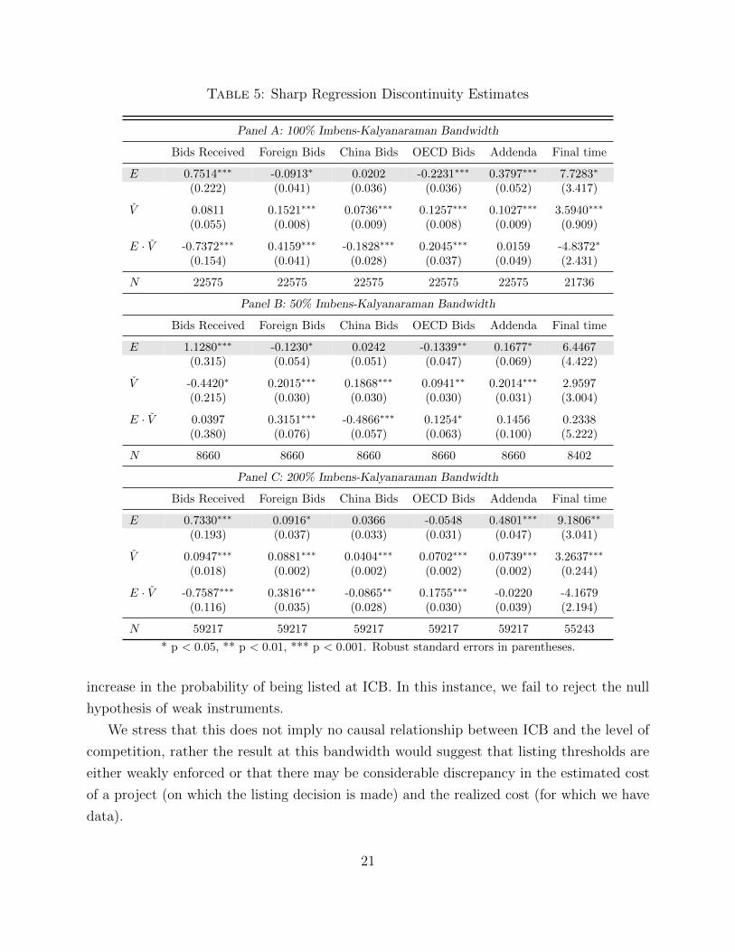
Table 5: Sharp Regression Discontinuity Estimates
Panel A: 100% Imbens-Kalyanaraman Bandwidth
Bids Received Foreign Bids China Bids OECD Bids Addenda Final time
E 0.7514∗∗∗ -0.0913∗ 0.0202 -0.2231∗∗∗ 0.3797∗∗∗ 7.7283∗
(0.222) (0.041) (0.036) (0.036) (0.052) (3.417)
V 0.0811 0.1521∗∗∗ 0.0736∗∗∗ 0.1257∗∗∗ 0.1027∗∗∗ 3.5940∗∗∗
(0.055) (0.008) (0.009) (0.008) (0.009) (0.909)
E · V -0.7372∗∗∗ 0.4159∗∗∗ -0.1828∗∗∗ 0.2045∗∗∗ 0.0159 -4.8372∗
(0.154) (0.041) (0.028) (0.037) (0.049) (2.431)
N 22575 22575 22575 22575 22575 21736
Panel B: 50% Imbens-Kalyanaraman Bandwidth
Bids Received Foreign Bids China Bids OECD Bids Addenda Final time
E 1.1280∗∗∗ -0.1230∗ 0.0242 -0.1339∗∗ 0.1677∗ 6.4467(0.315) (0.054) (0.051) (0.047) (0.069) (4.422)
V -0.4420∗ 0.2015∗∗∗ 0.1868∗∗∗ 0.0941∗∗ 0.2014∗∗∗ 2.9597(0.215) (0.030) (0.030) (0.030) (0.031) (3.004)
E · V 0.0397 0.3151∗∗∗ -0.4866∗∗∗ 0.1254∗ 0.1456 0.2338(0.380) (0.076) (0.057) (0.063) (0.100) (5.222)
N 8660 8660 8660 8660 8660 8402
Panel C: 200% Imbens-Kalyanaraman Bandwidth
Bids Received Foreign Bids China Bids OECD Bids Addenda Final time
E 0.7330∗∗∗ 0.0916∗ 0.0366 -0.0548 0.4801∗∗∗ 9.1806∗∗
(0.193) (0.037) (0.033) (0.031) (0.047) (3.041)
V 0.0947∗∗∗ 0.0881∗∗∗ 0.0404∗∗∗ 0.0702∗∗∗ 0.0739∗∗∗ 3.2637∗∗∗
(0.018) (0.002) (0.002) (0.002) (0.002) (0.244)
E · V -0.7587∗∗∗ 0.3816∗∗∗ -0.0865∗∗ 0.1755∗∗∗ -0.0220 -4.1679(0.116) (0.035) (0.028) (0.030) (0.039) (2.194)
N 59217 59217 59217 59217 59217 55243
* p < 0.05, ** p < 0.01, *** p < 0.001. Robust standard errors in parentheses.
increase in the probability of being listed at ICB. In this instance, we fail to reject the null
hypothesis of weak instruments.
We stress that this does not imply no causal relationship between ICB and the level of
competition, rather the result at this bandwidth would suggest that listing thresholds are
either weakly enforced or that there may be considerable discrepancy in the estimated cost
of a project (on which the listing decision is made) and the realized cost (for which we have
data).
21
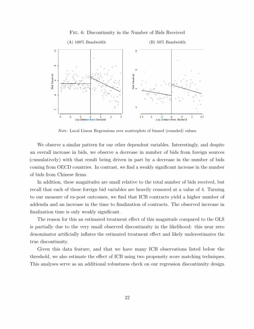
Fig. 6: Discontinuity in the Number of Bids Received
(A) 100% Bandwidth (B) 50% Bandwidth
Note: Local Linear Regressions over scatterplots of binned (rounded) values.
We observe a similar pattern for our other dependent variables. Interestingly, and despite
an overall increase in bids, we observe a decrease in number of bids from foreign sources
(cumulatively) with that result being driven in part by a decrease in the number of bids
coming from OECD countries. In contrast, we find a weakly significant increase in the number
of bids from Chinese firms.
In addition, these magnitudes are small relative to the total number of bids received, but
recall that each of these foreign bid variables are heavily censored at a value of 4. Turning
to our measure of ex-post outcomes, we find that ICB contracts yield a higher number of
addenda and an increase in the time to finalization of contracts. The observed increase in
finalization time is only weakly significant.
The reason for this an estimated treatment effect of this magnitude compared to the OLS
is partially due to the very small observed discontinuity in the likelihood: this near zero
denominator artificially inflates the estimated treatment effect and likely underestimates the
true discontinuity.
Given this data feature, and that we have many ICB observations listed below the
threshold, we also estimate the effect of ICB using two propensity score matching techniques.
This analyses serve as an additional robustness check on our regression discontinuity design.
22
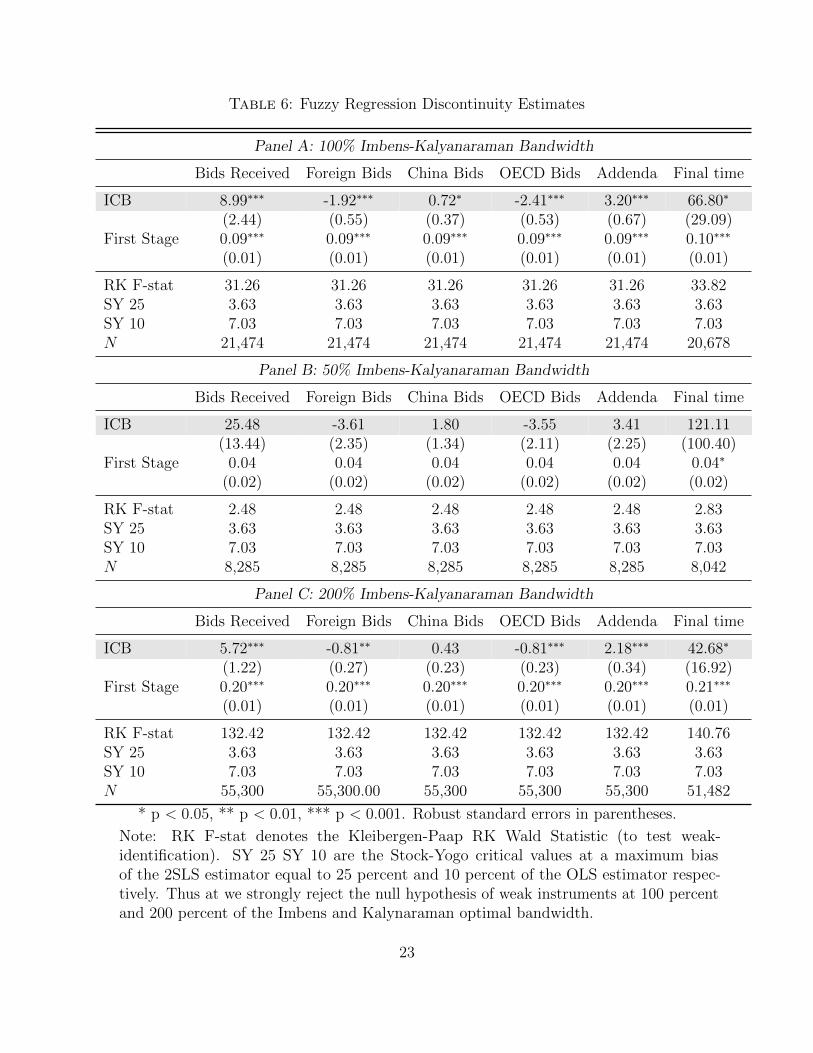
Table 6: Fuzzy Regression Discontinuity Estimates
Panel A: 100% Imbens-Kalyanaraman Bandwidth
Bids Received Foreign Bids China Bids OECD Bids Addenda Final time
ICB 8.99∗∗∗ -1.92∗∗∗ 0.72∗ -2.41∗∗∗ 3.20∗∗∗ 66.80∗
(2.44) (0.55) (0.37) (0.53) (0.67) (29.09)First Stage 0.09∗∗∗ 0.09∗∗∗ 0.09∗∗∗ 0.09∗∗∗ 0.09∗∗∗ 0.10∗∗∗
(0.01) (0.01) (0.01) (0.01) (0.01) (0.01)
RK F-stat 31.26 31.26 31.26 31.26 31.26 33.82SY 25 3.63 3.63 3.63 3.63 3.63 3.63SY 10 7.03 7.03 7.03 7.03 7.03 7.03N 21,474 21,474 21,474 21,474 21,474 20,678
Panel B: 50% Imbens-Kalyanaraman Bandwidth
Bids Received Foreign Bids China Bids OECD Bids Addenda Final time
ICB 25.48 -3.61 1.80 -3.55 3.41 121.11(13.44) (2.35) (1.34) (2.11) (2.25) (100.40)
First Stage 0.04 0.04 0.04 0.04 0.04 0.04∗
(0.02) (0.02) (0.02) (0.02) (0.02) (0.02)
RK F-stat 2.48 2.48 2.48 2.48 2.48 2.83SY 25 3.63 3.63 3.63 3.63 3.63 3.63SY 10 7.03 7.03 7.03 7.03 7.03 7.03N 8,285 8,285 8,285 8,285 8,285 8,042
Panel C: 200% Imbens-Kalyanaraman Bandwidth
Bids Received Foreign Bids China Bids OECD Bids Addenda Final time
ICB 5.72∗∗∗ -0.81∗∗ 0.43 -0.81∗∗∗ 2.18∗∗∗ 42.68∗
(1.22) (0.27) (0.23) (0.23) (0.34) (16.92)First Stage 0.20∗∗∗ 0.20∗∗∗ 0.20∗∗∗ 0.20∗∗∗ 0.20∗∗∗ 0.21∗∗∗
(0.01) (0.01) (0.01) (0.01) (0.01) (0.01)
RK F-stat 132.42 132.42 132.42 132.42 132.42 140.76SY 25 3.63 3.63 3.63 3.63 3.63 3.63SY 10 7.03 7.03 7.03 7.03 7.03 7.03N 55,300 55,300.00 55,300 55,300 55,300 51,482
* p < 0.05, ** p < 0.01, *** p < 0.001. Robust standard errors in parentheses.
Note: RK F-stat denotes the Kleibergen-Paap RK Wald Statistic (to test weak-identification). SY 25 SY 10 are the Stock-Yogo critical values at a maximum biasof the 2SLS estimator equal to 25 percent and 10 percent of the OLS estimator respec-tively. Thus at we strongly reject the null hypothesis of weak instruments at 100 percentand 200 percent of the Imbens and Kalynaraman optimal bandwidth.
23
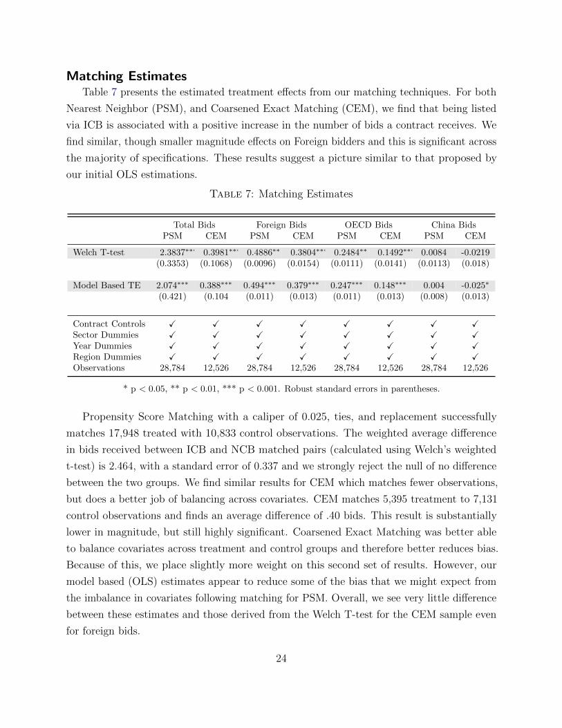
Matching EstimatesTable 7 presents the estimated treatment effects from our matching techniques. For both
Nearest Neighbor (PSM), and Coarsened Exact Matching (CEM), we find that being listed
via ICB is associated with a positive increase in the number of bids a contract receives. We
find similar, though smaller magnitude effects on Foreign bidders and this is significant across
the majority of specifications. These results suggest a picture similar to that proposed by
our initial OLS estimations.
Table 7: Matching Estimates
Total Bids Foreign Bids OECD Bids China BidsPSM CEM PSM CEM PSM CEM PSM CEM
Welch T-test 2.3837∗∗∗ 0.3981∗∗∗ 0.4886∗∗ 0.3804∗∗∗ 0.2484∗∗ 0.1492∗∗∗ 0.0084 -0.0219(0.3353) (0.1068) (0.0096) (0.0154) (0.0111) (0.0141) (0.0113) (0.018)
Model Based TE 2.074∗∗∗ 0.388∗∗∗ 0.494∗∗∗ 0.379∗∗∗ 0.247∗∗∗ 0.148∗∗∗ 0.004 -0.025∗
(0.421) (0.104 (0.011) (0.013) (0.011) (0.013) (0.008) (0.013)
Contract Controls X X X X X X X XSector Dummies X X X X X X X XYear Dummies X X X X X X X XRegion Dummies X X X X X X X XObservations 28,784 12,526 28,784 12,526 28,784 12,526 28,784 12,526
* p < 0.05, ** p < 0.01, *** p < 0.001. Robust standard errors in parentheses.
Propensity Score Matching with a caliper of 0.025, ties, and replacement successfully
matches 17,948 treated with 10,833 control observations. The weighted average difference
in bids received between ICB and NCB matched pairs (calculated using Welch’s weighted
t-test) is 2.464, with a standard error of 0.337 and we strongly reject the null of no difference
between the two groups. We find similar results for CEM which matches fewer observations,
but does a better job of balancing across covariates. CEM matches 5,395 treatment to 7,131
control observations and finds an average difference of .40 bids. This result is substantially
lower in magnitude, but still highly significant. Coarsened Exact Matching was better able
to balance covariates across treatment and control groups and therefore better reduces bias.
Because of this, we place slightly more weight on this second set of results. However, our
model based (OLS) estimates appear to reduce some of the bias that we might expect from
the imbalance in covariates following matching for PSM. Overall, we see very little difference
between these estimates and those derived from the Welch T-test for the CEM sample even
for foreign bids.
24

Looking at figure 12 –a visualization of the sharp RD with binned averages disaggregated by
listing status– we also note that in the case of Foreign Bids and OECD bids, the RD estimates
obscure some of the underlying trends in the data. For both of these outcome variables we
observe that the number of bidders is almost uniformly higher for ICB observations within
value categories. The high volume of ICB observations below this cutoff (coupled with a
non-linear trend) leads to the effect being averaged out.
Additionally, we reconcile the differences between our regression discontinuity estimates
and our matching estimates with the differences between average treatment on the treated
and local average treatment effects (ATT and LATE). Given the preponderance of ICB
observations that are below the threshold, the matching methodologies we employ here
will incorporate the differences between the dependent variables of ICB and NCB contracts
whose values are similarly far from the threshold in addition to those proximal to the cut-off.
These estimate the average treatment effect on the treated across the range of contracts.
ICB contracts below the threshold however are likely listed for reasons other than the size
of the contract. So while our matching estimators are non-localized and better able to
distinguish between treated and not-treated, they may be subject to bias due to selection
on unobservables. However, both of these methodologies identify a positive and significant
increase in the level of competition for contracts listed via more open procurement methods.
ConclusionWhile the results presented above are fragile and based on imperfect data, they are
suggestive of an economically meaningful impact of a reasonably limited increase in advertising
and transparency on procurement outcomes. In each of ordinary least squares regression,
regression discontinuity design, and several matching estimators, we find a significant increase
in the level of competition (bids) with an increase in advertising despite several data quality
issues and a number of potential biases. Our matching estimators suggest an increase in
the number of foreign bidders, driven mostly by OECD countries. These results suggest
a potential payoff to greater procurement transparency as advocated by groups including
the Open Contracting Partnership. Policy recommendations are fairly simple; increasing
advertising can improve competition and therefore procurement outcomes such as project
quality and price, though we are unable to directly test for these outcomes here.
Thus, there is substantial scope for further inquiry. A potential next stage of research
would be to investigate the effect of transparency on more closely monitored contracts. Namely,
does better and more open contract lead to improvements in outcomes and reductions in
25

costs. The Road Cost Knowledge System database from the World Bank collects detailed
information on the costs of road construction based on observable characteristics of the
style, size, material, and terrain across which the road will be built. Comparing across only
road projects would allow researchers to overcome many of the issues of comparability and
selection based on unobservable characteristics that we find in this paper.
26
ReferencesAfricon (2008). Unit costs of infrastructure projects in sub-saharan africa. Diagnostic, Africa
Infrastructure Country Background Paper, World Bank, Washington DC.
Caliendo, M. and Kopeinig, S. (2008). Some practical guidance for the implementation of
propensity score matching. Journal of economic surveys, 22(1):31–72.
Coviello, D. and Mariniello, M. (2014). Publicity requirements in public procurement:
Evidence from a regression discontinuity design. Journal of Public Economics, 109:76–100.
Estache, A. and Iimi, A. (2008). Procurement efficiency for infrastructure development and
financial needs reassessed. World Bank Policy Research Working Paper Series, Vol.
Galletta, S., Jametti, M., and Redonda, A. (2015). Highway to economic growth? competition
in public works tenders in the democratic republic of congo. South African Journal of
Economics, 83(2):240–252.
Hahn, J., Todd, P., and Van der Klaauw, W. (2001). Identification and estimation of
treatment effects with a regression-discontinuity design. Econometrica, 69(1):201–209.
Iacus, S. M., King, G., and Porro, G. (2011). Causal inference without balance checking:
Coarsened exact matching. Political analysis, page mpr013.
Iimi, A. (2006). Auction reforms for effective official development assistance. Review of
Industrial Organization, 28(2):109–128.
Imbens, G. and Kalyanaraman, K. (2011). Optimal bandwidth choice for the regression
discontinuity estimator. The Review of Economic Studies, page rdr043.
Kenny, C. (2010). Publishing construction contracts and outcome details. World Bank Policy
Research Working Paper Series, Vol.
Kenny, C. and Karver, J. (2012). Publish what you buy: the case for routine publica-
tion of government contracts. CGD Policy Paper 011 (Washington: Center for Global
Development).
Lee, D. S. and Lemieux, T. (2010). Regression discontinuity designs in economics. Journal
of Economic Literature, 48:281–355.
27
McCrary, J. (2008). Manipulation of the running variable in the regression discontinuity
design: A density test. Journal of Econometrics, 142(2):698–714.
Ohashi, H. (2009). Effects of transparency in procurement practices on government ex-
penditure: A case study of municipal public works. Review of Industrial Organization,
34(3):267–285.
Onur, I., Ozcan, R., and Tas, B. K. O. (2012). Public procurement auctions and competition
in turkey. Review of Industrial Organization, 40(3):207–223.
Pavel, J., Sicakova-Beblava, E., et al. (2013). Do e-auctions really improve the efficiency
of public procurement? the case of the slovak municipalities. Prague Economic Papers,
22(1):111–124.
Rosenbaum, P. R. and Rubin, D. B. (1983). The central role of the propensity score in
observational studies for causal effects. Biometrika, 70(1):41–55.
Smith, A. (1776). An inquiry into the nature and causes of the wealth of nations: Volume
one.
Soraya, G. (2009). Indonesian experience governance and anticorruption bali urban infras-
tructure project (buip) presentation to the world bank gac in projects group.
28
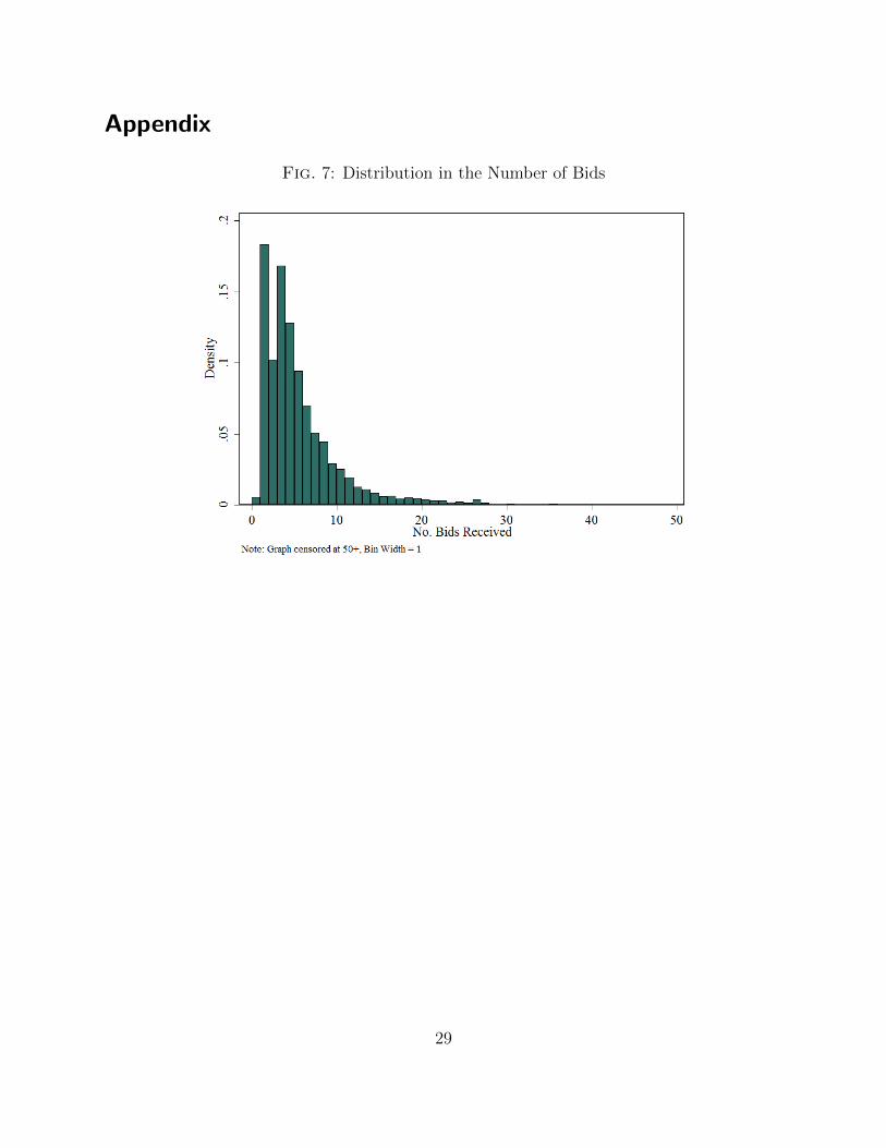
Appendix
Fig. 7: Distribution in the Number of Bids
29
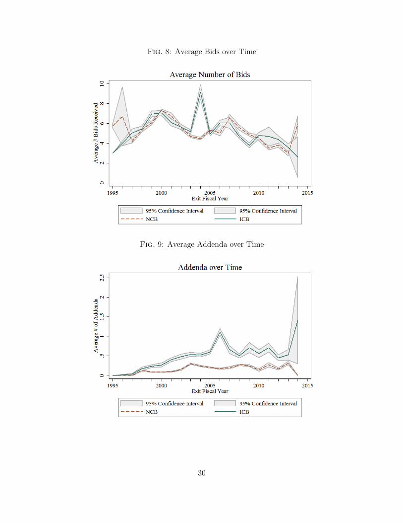
Fig. 8: Average Bids over Time
Fig. 9: Average Addenda over Time
30

Fig. 10: Average Time to Finalization
Fig. 11: Share of Total Contract Value by Procurement Method
31
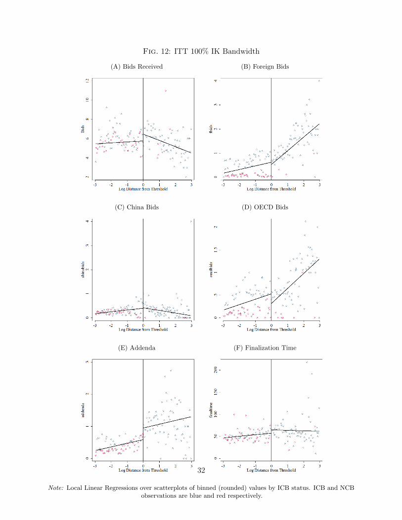
Fig. 12: ITT 100% IK Bandwidth
(A) Bids Received (B) Foreign Bids
(C) China Bids (D) OECD Bids
(E) Addenda (F) Finalization Time
Note: Local Linear Regressions over scatterplots of binned (rounded) values by ICB status. ICB and NCBobservations are blue and red respectively.
32
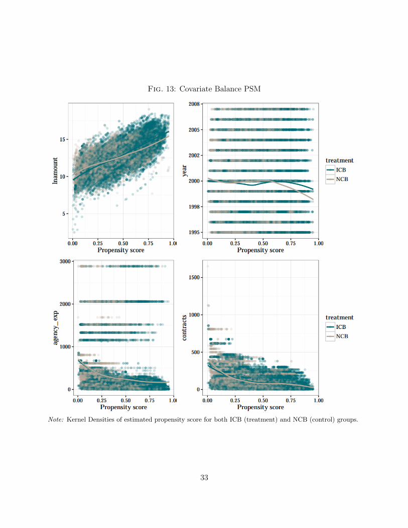
Fig. 13: Covariate Balance PSM
Note: Kernel Densities of estimated propensity score for both ICB (treatment) and NCB (control) groups.
33
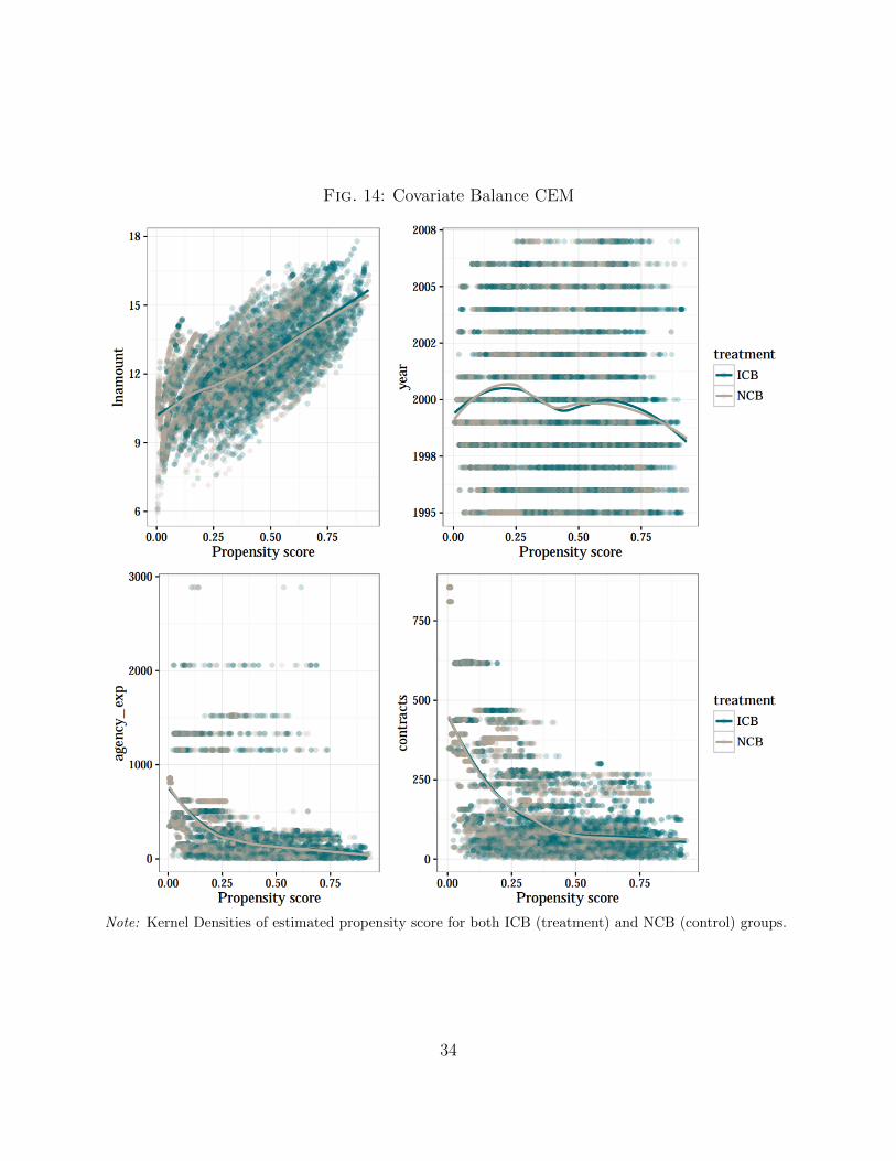
Fig. 14: Covariate Balance CEM
Note: Kernel Densities of estimated propensity score for both ICB (treatment) and NCB (control) groups.
34