working paper monetary policy, redistribution, and risk premia
TRANSCRIPT

5757 S. University Ave.
Chicago, IL 60637
Main: 773.702.5599
bfi.uchicago.edu
WORKING PAPER · NO. 2020-02
Monetary Policy, Redistribution, and Risk PremiaRohan Kekre and Moritz LenelMAY 2021
Monetary Policy, Redistribution,and Risk Premia∗
Rohan Kekre† Moritz Lenel‡
May 2021
Abstract
We study the transmission of monetary policy through risk premia in a het-
erogeneous agent New Keynesian environment. Heterogeneity in households’
marginal propensity to take risk (MPR) summarizes differences in portfolio choice
on the margin. An unexpected reduction in the nominal interest rate redis-
tributes to households with high MPRs, lowering risk premia and amplifying the
stimulus to the real economy. Quantitatively, this mechanism rationalizes the
role of news about future excess returns in driving the stock market response to
monetary policy shocks and amplifies their real effects by 1.3-1.5 times.
JEL codes: E44, E52, G12
Keywords: monetary policy, risk premia, heterogeneous agents
∗We thank Fernando Alvarez, Adrien Auclert, Markus Brunnermeier, Emmanuel Farhi, GitaGopinath, Francois Gourio, Veronica Guerrieri, Zhiguo He, Erik Hurst, Anil Kashyap, Nobu Kiyotaki,Stefan Nagel, Brent Neiman, Stavros Panageas, Juan Passadore, Greg Phelan, Monika Piazzesi, Mar-tin Schneider, Alp Simsek, Ludwig Straub, Gianluca Violante, Ivan Werning, Tom Winberry, andMoto Yogo for discussions. We thank Jihong Song and Menglu Xu for research assistance.†Chicago Booth and NBER. Email: [email protected].‡Princeton. Email: [email protected].
1 Introduction
A growing literature finds that expansionary monetary policy lowers risk premia. This
has been established for the equity premium in stock markets, the term premium
in nominal bonds, and the external finance premium on risky corporate debt.1 The
basic New Keynesian framework as in Woodford (2003) and Gali (2008) does not
capture this aspect of monetary policy transmission. As noted by Kaplan and Violante
(2018), this is equally true for emerging heterogeneous agent New Keynesian models in
which heterogeneity in the marginal propensity to consume enriches the transmission
mechanism but still cannot explain the associated movements in risk premia.
This paper demonstrates that a New Keynesian model with heterogeneous house-
holds differing instead in risk-bearing capacity can quantitatively rationalize the ob-
served effects of policy on risk premia, amplifying the transmission to the real economy.
An expansionary monetary policy shock lowers the risk premium on capital if it redis-
tributes to households with a high marginal propensity to take risk (MPR), defined as
the marginal propensity to save in capital relative to save overall. With heterogeneity
in risk aversion, portfolio constraints, rules of thumb, background risk, or beliefs, high
MPR households borrow in the bond market from low MPR households to hold lever-
aged positions in capital. By generating unexpected inflation, raising profit income
relative to labor income, and raising the price of capital, an expansionary monetary
policy shock redistributes to high MPR households and thus lowers the market price
of risk. In a calibration matching portfolio heterogeneity in the U.S. economy, this
rationalizes the observed role of news about lower future excess returns in driving the
increase in the stock market. The real stimulus is amplified by 1.3-1.5 times relative
to a representative agent economy without heterogeneity in portfolios and MPRs.
Our baseline environment enriches a standard New Keynesian model with Epstein
and Zin (1991) preferences and heterogeneity in risk aversion. Households consume,
supply labor subject to adjustment costs in nominal wages, and choose a portfolio of
nominal bonds and capital. Production is subject to aggregate TFP shocks. Monetary
policy follows a Taylor (1993) rule. Heterogeneity in risk aversion generates hetero-
geneity in MPRs and exposures to a monetary policy shock. Epstein-Zin preferences
allow us to flexibly model this heterogeneity as distinct from households’ intertempo-
ral elasticities of substitution. We begin by analytically characterizing the effects of a
monetary policy shock in a simple two-period version of this environment, providing an
1See Bernanke and Kuttner (2005), Hanson and Stein (2015), and Gertler and Karadi (2015).
1

organizing framework for the quantitative analysis of the infinite horizon which follows.
An expansionary monetary policy shock lowers the risk premium by redistributing
wealth to households with a high marginal propensity to save in capital relative to save
overall — that is, a high MPR. Redistribution to high MPR households lowers the risk
premium because of asset market clearing: if households on aggregate wish to increase
their portfolio share in capital, its expected return must fall relative to that on bonds.
An expansionary monetary policy shock redistributes across households by revaluing
their initial balance sheets: it deflates nominal debt, raises the profits earned using
capital, and raises the price of capital. More risk tolerant households hold leveraged
positions in capital and have a higher MPR. Hence, an expansionary monetary policy
shock will redistribute to these households and lower the risk premium.
The reduction in the risk premium amplifies the transmission of monetary policy to
the real economy. Conditional on the real interest rate — which reflects the degree of
nominal rigidity and the monetary policy rule — a decline in the required excess return
on capital is associated with an increase in investment. The increase in investment
crowds in consumption by raising household wealth. The stimulus to consumption and
investment implies an increase in output overall.
These results are robust to heterogeneity beyond risk aversion. We consider a richer
environment in which households may also face portfolio constraints or follow rules-of-
thumb; households may be subject to idiosyncratic background risk; and households
may have subjective beliefs regarding the value of capital. Because each of these forms
of heterogeneity imply that households holding more levered positions in capital will be
the ones with a high MPR, they continue to imply that expansionary monetary policy
will lower the risk premium through redistribution, amplifying real transmission.
Accounting for the risk premium effects of monetary policy is important given em-
pirical evidence implying that it may be a key component of the transmission mecha-
nism. We refresh this point from Bernanke and Kuttner (2005) using the structural vec-
tor autoregression instrumental variables (SVAR-IV) approach in Gertler and Karadi
(2015). We find that a monetary policy shock resulting in a roughly 0.2pp reduction in
the 1-year Treasury yield leads to a 2pp increase in the real S&P 500 return. Using a
Campbell and Shiller (1988) decomposition and accounting for estimation uncertainty,
20%− 100% of this increase is driven by lower future excess returns, challenging exist-
ing New Keynesian frameworks where essentially all of the effect on the stock market
operates instead through higher dividends or lower risk-free rates.
2
Extending the model to the infinite horizon, we investigate whether a calibration to
the U.S. economy is capable of rationalizing these facts. We match the heterogeneity in
wealth, labor income, and financial portfolios in the Survey of Consumer Finances, to-
gether disciplining the exposures to a monetary policy shock and MPRs. We use global
solution methods to solve the model. To make the computational burden tractable,
we model three groups of households: two groups corresponding to the small fraction
with high wealth relative to labor income, but differing in their risk tolerance and thus
portfolio share in capital, and one group corresponding to the large fraction holding
little wealth relative to labor income. In the data, the high-wealth, high-leverage group
is disproportionately composed of households with private business wealth, while the
high-wealth, low-leverage group is disproportionately composed of retirees.
We find that the redistribution across households with heterogeneous MPRs can
quantitatively explain the risk premium effects of an expansionary monetary policy
shock. Notably, the redistribution relevant for this result is between wealthy households
holding heterogeneous portfolios, rather than between the asset-poor and asset-rich.
Using the same Campbell-Shiller decomposition as was used on the data, 33% of the
return on equity in our baseline parameterization arises from news about lower future
excess returns, compared to 0% in a representative agent counterfactual. Consistent
with the analytical results, the redistribution to high-MPR households is amplified
with a more persistent shock and thus larger debt deflation; higher stickiness and
thus a larger increase in profit income relative to labor income; or higher investment
adjustment costs and thus a larger increase in the price of capital.
Further consistent with the analytical results, the reduction in the risk premium
through redistribution in turn amplifies the effect of policy on the real economy. In both
our baseline and counterfactual representative agent economies, we solve for monetary
policy shocks which deliver a 0.2pp decline in the 1-year nominal yield on impact.
Given these shocks, our model amplifies the response of quantities by 1.3-1.5 times:
the peak investment, consumption, and output responses are 2.3pp, 0.5pp, and 0.9pp,
while the counterparts in the representative agent economy are 1.6pp, 0.3pp, and 0.6pp.
Related literature Our paper contributes to the rapidly growing literature on het-
erogeneous agent New Keynesian (HANK) models by studying the transmission of
monetary policy through risk premia. We build on Doepke and Schneider (2006) in
our measurement of household portfolios, informing the heterogeneity in exposures to a
3
monetary policy shock. The redistributive effects of monetary policy in our framework
follow Auclert (2019). We demonstrate that it is the covariance of these exposures with
MPRs rather than MPCs which matters for policy transmission through risk premia.
Like Kaplan, Moll, and Violante (2018) and Luetticke (2021), we study a two-asset en-
vironment with bonds and capital. And like Alves, Kaplan, Moll, and Violante (2020),
Auclert, Rognlie, and Straub (2020), and Melcangi and Sterk (2021) we study the ef-
fects of monetary policy shocks on asset prices. Unlike these models, in our framework
assets differ in their exposure to aggregate risk rather than in their liquidity, allowing
us to account for the important role of risk premia in driving the change in asset prices.
In doing so, we bring to the HANK literature many established insights from het-
erogeneous agent and intermediary-based asset pricing. The wealth distribution is a
crucial determinant of the market price of risk as in other models with heterogeneous
risk aversion (e.g., Garleanu and Panageas (2015)), segmented markets (e.g., He and
Krishnamurthy (2013)), rules-of-thumb (e.g., Chien, Cole, and Lustig (2012)), back-
ground risk (e.g., Constantinides and Duffie (1996)), or heterogeneous beliefs (e.g.,
Geanakoplos (2009)).2 We build on this literature by focusing on the changes in
wealth induced by a monetary policy shock in a production economy with nominal
rigidities. In studying this question we follow Alvarez, Atkeson, and Kehoe (2009) and
Drechsler, Savov, and Schnabl (2018), who study the effects of monetary policy on
risk premia in an exchange economy with segmented markets and in a model of bank-
ing, respectively.3 We instead study these effects operating through the revaluation of
heterogeneous agents’ balance sheets in a conventional New Keynesian setting.
Indeed, our paper most directly builds on prior work focused on risk premia in New
Keynesian economies. We clarify the sense in which Bernanke, Gertler, and Gilchrist
(1999) served as a seminal HANK model focused on heterogeneity in MPRs rather
than MPCs.4 As we demonstrate, however, heterogeneity in MPRs need not rely
2In recent work, Panageas (2020) studies the common structure and implications of these models,and Toda and Walsh (2020) emphasize portfolio heterogeneity as a summary statistic to evaluate theeffects of redistribution with incomplete markets, as in our analysis.
3More recently, Bhandari, Evans, and Golosov (2019) construct a segmented markets model inthe spirit of Alvarez et al. (2009) in which monetary policy also has effects on risk premia. Chen andPhelan (2019) integrate the effects of monetary policy on risk premia in Drechsler et al. (2018) withthe macroeconomic framework of Brunnermeier and Sannikov (2014) to study the effects of monetarypolicy on financial stability. Coimbra and Rey (2020) study the effects of changes in interest rates onrisk premia and financial stability in a model with heterogeneous intermediaries.
4In Bernanke et al. (1999), households can only trade bonds while entrepreneurs can trade bondsand capital. In equilibrium, households have a zero MPR while entrepreneurs have a positive MPR.Changes in net worth across these agents thus affects credit spreads and economic activity.
4
on market segmentation, justifying its relevance even in markets which may not be
intermediated by specialists. In relating movements in the risk premium to the real
economy, we make use of the insight in Ilut and Schneider (2014), Caballero and Farhi
(2018), and Caballero and Simsek (2020) that an increase in the risk premium will
induce a recession if the safe interest rate does not sufficiently fall in response.5 We
build especially on the latter two papers, as well as Brunnermeier and Sannikov (2012,
2016), in emphasizing the effects of heterogeneity in asset valuations on risk premia.
Relative to these papers, we explore the importance of such heterogeneity for monetary
transmission in a calibration to the U.S. economy.6
Like all of these papers, our analysis also provides a theoretical counterpart to the
large empirical literature studying links between risky asset prices and real activity.
Focusing first on stock prices, the evidence in support of the q-theory of investment has
been mixed, and causal estimates of stock prices on consumption have been made diffi-
cult by the fact that they may simply be forecasting other determinants of consumption.
Recently, Pflueger, Siriwardane, and Sunderam (2020) and Chodorow-Reich, Nenov,
and Simsek (2020) have employed cross-sectional identification strategies to overcome
these challenges, finding evidence in support of the cost-of-capital and consumption
wealth mechanisms in our model. Moreover, taking a broader interpretation of our
model as studying the effect of monetary policy on risky claims on capital, there is
substantial evidence that spreads on risky corporate debt predict real activity (e.g.,
Gilchrist and Zakrajsek (2012) and Lopez-Salido, Stein, and Zakrajsek (2017)).
Outline In section 2 we characterize our main insights in a two-period environment.
In section 3 we compare empirical evidence on the equity market response to monetary
policy shocks to the quantitative predictions of our model enriched to the infinite
horizon and calibrated to the U.S. economy. Finally, in section 4 we conclude.
2 Analytical insights in a two-period environment
We first characterize our main conceptual insights in a two-period environment al-
lowing us to obtain simple analytical results. Heterogeneity in risk aversion induces
5While these authors make this point in the case of a time-varying price of risk (as in our model),a similar result obtains with a time-varying quantity of risk as in Fernandez-Villaverde, Guerron-Quintana, Kuester, and Rubio-Ramirez (2015), Basu and Bundick (2017), and DiTella (2020).
6In recent complementary work, Pflueger and Rinaldi (2021) study monetary transmission andrisk premia in a representative agent New Keynesian model augmented with consumption habits.
5

heterogeneity in household portfolios. An expansionary monetary policy shock lowers
the risk premium on capital by redistributing to relatively risk tolerant households.
A reduction in the risk premium amplifies the stimulus to investment, consumption,
and output. These results are robust to heterogeneity in rules-of-thumb, portfolio con-
straints, background risk, or beliefs. More generally, they hold whenever relatively
levered households, who benefit disproportionately from a monetary easing, have rela-
tively high propensities to save in capital relative to bonds — i.e., high MPRs.
2.1 Environment
There are two periods, 0 and 1. To isolate the key mechanisms, we make a number of
parametric assumptions which are relaxed later in the paper.
Households A unit measure of households indexed by i ∈ [0, 1] have Epstein-Zin
preferences over consumption in each period {ci0, ci1} and labor supply `0
log vi0 = (1− β) log ci0 − θ`1+1/θ0
1 + 1/θ+ β log
(E0
[(ci1)
1−γi]) 1
1−γi, (1)
with a unitary intertemporal elasticity of substitution, discount factor β, relative risk
aversion γi, (dis)utility of labor θ, and Frisch elasticity θ. Labor in period 0 is not
indexed by i because (as we describe below) households supply the same amount. In
period 1 production only uses capital and thus there is no labor supplied.
In addition to consuming and supplying labor, the household chooses its position
in a nominal bond Bi0 and in capital ki0 subject to the resource constraints
P0ci0 +Bi
0 +Q0ki0 ≤ W0`0 + (1 + i−1)B
i−1 + (Π0 + (1− δ0)Q0)k
i−1, (2)
P1ci1 ≤ (1 + i0)B
i0 + Π1k
i0. (3)
Bi−1 and ki−1 are its endowments in these same assets. The consumption good trades
at Pt units of the nominal unit of account (“dollars”) at t,7 the household earns a
wage W0 dollars in period 0, one dollar in bonds purchased at t yields 1 + it dollars at
t+ 1, and one unit of capital purchased for Qt dollars at t yields a dividend Πt+1 plus
(1− δt+1)Qt+1 dollars at t+ 1. Capital fully depreciates after period 1 (δ1 = 1).
7Following Woodford (2003), we model the economy at the cashless limit.
6
Supply-side The nominal wage is rigid at its level set the previous period
W0 = W−1. (4)
Each household is willing to supply the labor demanded of it from firms, appealing to
households’ market power in the labor market which we spell out later in the paper.
In period 0, the representative producer hires `0 units of labor and rents k−1 units
of capital from households to produce the final good with TFP of one. It also uses(k0k−1
)χxx0 units of the consumption good to produce x0 new capital sold to households,
where χx indexes adjustment costs and it takes k0 as given. The producer thus earns
Π0k−1 = P0`1−α0 kα−1 −W0`0 +Q0x0 − P0
(k0k−1
)χxx0. (5)
In period 1, the producer rents k0 units of capital and has TFP exp(εz1), so it earns
Π1k0 = P1 exp(εz1)kα0 . (6)
Future TFP is uncertain in period 0, following
εz1 ∼ N
(−1
2σ2, σ2
). (7)
Policy The government sets monetary policy {i0, P1} by committing to P1 = P0,
eliminating inflation risk in the nominal bond,8 and following the Taylor rule
1 + i0 = (1 + i)
(P0
P−1
)φexp(εm0 ) (8)
with reference price P−1, where εm0 is the shock of interest. It follows that the real
interest rate between periods 0 and 1 is9
1 + r1 ≡ (1 + i0)P0
P1
= (1 + i)
(P0
P−1
)φexp(εm0 ).
8It is straightforward to allow P1 = P0 exp(ιεz1) for ι 6= 0, so that there is inflation risk in thenominal bond. Our quantitative analysis in the next section features inflation risk.
9Between periods t and t + 1 we denote it the nominal interest rate known in period t and rt+1
the realized real interest rate depending on the price level in period t+ 1.
7
Market clearing Market clearing in goods is∫ 1
0
ci0di+
(k0k−1
)χxx0 = `1−α0 kα−1,
∫ 1
0
ci1di = exp(εz1)kα0 , (9)
in the capital rental market is∫ 1
0
ki−1di = k−1,
∫ 1
0
ki0di = k0, (10)
in the capital claims market is
(1− δ0)∫ 1
0
ki−1di+ x0 =
∫ 1
0
ki0di, (11)
and in bonds is ∫ 1
0
Bi0di = 0. (12)
Equilibrium Given the state variables {W−1, P−1, {Bi−1, k
i−1}, i−1, εm0 } and a stochas-
tic process for εz1 in (7), the definition of equilibrium is then standard:
Definition 1. An equilibrium is a set of prices and policies such that: (i) each house-
hold i chooses {ci0, Bi0, k
i0, c
i1} to maximize (1) subject to (2)-(3), (ii) wages are rigid
as in (4), (iii) the representative producer chooses {`0, x0} to maximize profits (5) and
earns profits (6), (iv) the government sets {i0, P1} according to P1 = P0 and (8), and
(v) the goods, capital, and bond markets clear according to (9)-(12).
We now characterize the comparative statics of this economy with respect to a
monetary policy shock εm0 in a sequence of three main propositions. Each result builds
on the last, and each makes use of only a few equilibrium conditions.
2.2 Monetary policy, redistribution, and the risk premium
We first provide a general result characterizing the effect of a monetary policy shock
on the expected excess return on capital.
We need to know each household’s chosen portfolio in capital. Define i’s real savings
ai0 ≡ bi0 + q0ki0,
8

and portfolio share in capital
ωi0 ≡q0k
i0
ai0,
where we use lower-case to denote the real analogs to the nominal variables introduced
earlier. Let 1 + rk1 denote the gross real returns on capital
1 + rk1 ≡Π1
Q0
P0
P1
=π1q0.
Then i’s optimality condition for ωi0 is given by
E0
[(ci1)−γi
(rk1 − r1)]
= 0. (13)
Taking a Taylor approximation of the expression inside the expectation up to second
order in the excess log return, it follows that the optimal portfolio share in capital
approximately satisfies
ωi0 ≈1
γiE0 log(1 + rk1)− log(1 + r1) + 1
2σ2
σ2. (14)
Given a positive risk premium, more risk tolerant households choose a larger portfolio
share in capital. This is the only approximation we use in the results which follow.
Simply by aggregating (14) and making use of the asset market clearing conditions
(10) and (12), we obtain the first result of the paper, the proof of which (along with
all other proofs) is in appendix A:
Proposition 1. The risk premium on capital is
E0 log(1 + rk1)− log(1 + r1) +1
2σ2 = γσ2,
where
γ ≡
(∫ 1
0
ai0∫ 1
0ai′0 di′
1
γidi
)−1.
The change in the risk premium in response to a monetary shock is
d[E0 log(1 + rk1)− log(1 + r1)
]dεm0
= γσ2
∫ 1
0
d[ai0/∫ 1
0ai′0 di′]
dεm0
(1− ωi0
)di. (15)
9

Hence, a monetary policy shock affects the risk premium if it redistributes across
households with heterogeneous portfolios. If monetary policy does not redistribute
(d[ai0/∫ 1
0ai′0 di′] /dεm0 = 0 for all i) or households have identical portfolios (ωi0 = 1 for
all i), there is no effect on the risk premium. Away from this case, redistributing wealth
to households with relatively high desired portfolios in capital lowers the risk premium.
Intuitively, such redistribution raises the relative demand for capital, lowering the
required excess return to clear asset markets.
2.3 Risk premium and the real economy
We now characterize why policy transmission through the risk premium is relevant for
the real economy.
The link between investment and the risk premium is due to the relation between
the expected return to capital and investment. Indeed, optimal investment solving (5)
and equilibrium dividends in (6) together imply that the expected return on capital is
given by
E0 log(1 + rk1) = logα + E0 log z1 + χx log k−1 − (1− α + χx) log k0. (16)
Hence, investment is declining in the expected return to capital.
The link between consumption and the risk premium is due to capital in households’
wealth. Indeed, household i’s optimal choice of consumption is given by
ci0 = (1− β)ni0(w0`0, P0, π0, q0),
where we collect i’s wealth as a function of non-predetermined variables in
ni0(w0`0, P0, π0, q0) ≡ w0`0 +1
P0
(1 + i−1)Bi−1 + (π0 + (1− δ0)q0)ki−1. (17)
Aggregating and making use of firms’ resource constraint (5) and the market clearing
conditions (9)-(12), we thus obtain:
Proposition 2. The change in investment in response to a monetary shock is
dk0dεm0
= − k01− α + χx
[d[E0 log(1 + rk1)− log(1 + r1)
]dεm0
+d log(1 + r1)
dεm0
]. (18)
10

The change in consumption c0 ≡∫ 1
0ci0di in response to a monetary shock is
dc0dεm0
=1− ββ
q0(1 + χx)dk0dεm0
.
The change in output y0 ≡ (`0)1−αkα−1 in response to a monetary shock is
dy0dεm0
=dc0dεm0
+ q0
(1 + χx
x0k0
)dk0dεm0
. (19)
Thus, conditional on the response of the real interest rate to a monetary shock, a
decline in the risk premium is associated with a decline in the required return on capital
and thus an increase in investment. The increase in investment in turn stimulates
consumption. Together, these stimulate output. These results apply to the case of a
monetary policy shock the more general insights of Caballero and Simsek (2020) linking
risk premia and the real economy.
2.4 Monetary transmission via the risk premium
We now sign the effects of a monetary policy shock on the risk premium and its
implications for the real economy.
The relevant measure of redistribution toward household i in Proposition 1 is the
change in its savings share. Since agents share the same marginal propensity to save
(β), this is equal to the change in its wealth share
d[ai0/∫ 1
0ai′0 di′]
dεm0=d[ni0/
∫ 1
0ni′0 di′]
dεm0. (20)
Given (17) and defining n0 ≡∫ 1
0ni0di, the change in its wealth share is in turn
d[ni0/
∫ 1
0ni′0 di′]
dεm0=
1
n0
[−1 + i−1
P0
Bi−1d logP0
dεm0+
(ki−1 −
ni0n0
k−1
)(dπ0dεm0
+ (1− δ) dq0dεm0
)]. (21)
Hence, in this setting there are three channels through which wealth is redistributed
on impact of a monetary policy shock: via inflation (which redistributes towards nom-
inal borrowers) or via an increase in profits or the price of capital (which redistribute
11

towards those with a disproportionate claim on capital). These heterogeneous expo-
sures to a monetary shock have been previously exposited in the HANK literature, as
by Auclert (2019). Propositions 1 and 2 imply that it is their covariance with portfolio
shares which matters for transmission through risk premia.
When agents’ initial endowments are consistent with their chosen portfolios in pe-
riod 0 — as would be the case in the steady-state of an infinite horizon model — and
they start with same initial levels of wealth, we can sharply sign these effects:
Proposition 3. Suppose agents differ in risk aversion {γi}; their initial endowments
are consistent with their chosen portfolio in period 0 ({ωi−1 = ωi0}); and they have the
same initial levels of wealth. Then:
• a cut in the nominal interest rate lowers the risk premium, and
• the resulting stimulus to investment, consumption, and output are larger than a
representative agent economy starting from the same aggregate allocation.
Intuitively, relatively risk tolerant agents finance levered positions in capital by
borrowing in nominal bonds. A cut in the nominal interest rate generates inflation,
an increase in profits, and an increase in the price of capital, redistributing wealth to
these agents. Proposition 1 implies that this lowers the risk premium. At least given
a conventional Taylor rule, the endogenous response of the real interest rate is not
sufficiently strong to overturn the amplification characterized in Proposition 2.
2.5 Other sources of heterogeneity
The preceding results do not rely on heterogeneity in risk aversion alone; they also
apply when there is heterogeneity in portfolios arising from other primitives.
Binding constraints or rules-of-thumb Suppose a measure of households are not
at an interior optimum in their portfolio choice because of the additional constraint
q0ki0 = ωi0a
i0,
reflecting either a binding leverage constraint or a rule-of-thumb in portfolios. When
ωi0 = 0 in particular, this means the household cannot participate in the capital market.
Such constraints are consistent with prior asset pricing models with segmented markets
or rules-of-thumb as well as macro models of the financial accelerator.
12
Background risk Suppose households are subject to idiosyncratic risk beyond the
aggregate risk already described: their capital chosen in period 0 is subject to a shock
εi1 in period 1, modeled as a multiplicative change in the efficiency units of capital.10
εi1 is iid across households and independent of the aggregate TFP shock εz1, and ηi
controls the degree of background risk according to
log εi1 ∼ N
(−1
2ηiσ2, ηiσ2
).
This environment captures features of the large literatures in macroeconomics and
finance with entrepreneurial income risk.
Subjective beliefs Suppose household i believes that TFP follows
εz1 ∼ N
(−1
2ς iσ2, ς iσ2
)even though the objective (true) probability distribution remains described by (7). As
in the large literature on belief disagreements, households with ς i > 1 are “pessimists”
and households with ς i < 1 are “optimists”.
We can then prove:
Proposition 4. Suppose households differ in risk aversion {γi}, being constrained and
(among those that are) constraints {ωi}, background risk {ηi}, and beliefs {ς i}. Further
suppose that their endowments are identical to their choices in period 0 and they are
otherwise identical. Then we obtain the same results as in Proposition 3.
Intuitively, in this more general environment a household’s portfolio share in capital
is falling in risk aversion γi, background risk ηi, and pessimism ς i, and rising in the
leverage constraint or rule-of-thumb ωi (if applicable). Regardless of these underlying
drivers, so long as households enter period 0 with endowments reflecting these same
portfolios, it will be the case that an expansionary monetary policy shock redistributes
to those wishing to hold relatively more capital. Thus, an expansionary shock lowers
the risk premium, amplifying the stimulus to the real economy.
10The assumption that εi1 scales the household’s return on capital differs from Krueger and Lustig(2010) in which idiosyncratic risk is instead on labor income.
13

2.6 Exposures and the marginal propensity to take risk
The robustness of these results derives from the tight link between households’ expo-
sures to a monetary policy shock and their marginal portfolio choices given a dollar of
income. In a more general environment, we now demonstrate that it is the covariance
between the two which governs the effects of such a shock on the risk premium.
Consider how a household’s optimal portfolio changes with an additional dollar of
income. Let the capital, bond, and total savings policy functions solving each house-
hold’s micro-level optimization problem be given by ki0(·), bi0(·), and ai0(·), respectively.
Their arguments are the household’s wealth ni0 and all other aggregates which the
household takes as given, such as the real interest rate r1 and price of capital q0. Then:
Definition 2. Household i’s marginal propensity to take risk (MPR) is
mpri0 ≡q0∂k
i0/∂n
i0
∂ai0/∂ni0
.
The MPR summarizes the household’s marginal portfolio choice in capital. It cap-
tures a dimension of household behavior in principle orthogonal to the marginal propen-
sity to consume emphasized in prior work. Note that the following results also hold
when inflation risk renders the nominal bond risky; we give the MPR its name because
under any realistic calibration the payoff on capital is more risky than on bonds.
In the environment studied in the prior subsections, households’ marginal and equi-
librium portfolios are identical (mpri0 = ωi0). This is no longer the case if households
have a non-unitary elasticity of intertemporal substitution or supply labor in period
1. We can still obtain analytical results in this more general environment, however,
by studying the limit as aggregate risk falls to zero. In doing so, we apply techniques
developed by Devereux and Sutherland (2011) in the context of open-economy macroe-
conomics to the present heterogeneous agent environment and our particular statistics
of interest.11 Letting variables with bars denote values at the point of approxima-
tion without aggregate risk, and returning to the case without portfolio constraints,
rules-of-thumb, background risk, and belief differences for simplicity, we obtain:
11In particular, a second-order approximation to optimal portfolio choice and the method of un-determined coefficients implies households’ limiting portfolios. A similar approach to the partialderivatives of households’ first-order conditions with respect to ni0 implies households’ limiting MPRs.
14
Proposition 5. At the limit of zero aggregate risk, i’s portfolio share in capital is
ωi0 ≡q0k
i0
ai0=
(ci1
(1 + r1)ai0
)γ
γi− w1
(1 + r1)ai0, (22)
and its MPR is
mpri0 =γ
γi, (23)
where
γ =
[∫ 1
0
ci1∫ 1
0ci′1 di′
1
γidi
]−1. (24)
is the harmonic average of risk aversion weighted by households’ future consumption.
This proposition naturally generalizes (14). Importantly and intuitively, it remains
that a household’s portfolio share in capital and its MPR are higher the less risk averse
it is relative to other households in the economy.12 Nonetheless, the portfolio share and
MPR are no longer the same: a household’s portfolio share in capital depends not only
on risk aversion but also its motive to hedge labor income also subject to TFP shocks,
captured by the last term in (22). This hedging motive is irrelevant on the margin.
The distinction between portfolios and MPRs is useful in clarifying their roles in a
generalization of Proposition 1, our final analytical result of the paper. Approximating
households’ optimal portfolio choice (13) and the asset market clearing conditions (10)
and (12) around the point with zero aggregate risk, and denoting with hats log/level
deviations from this point, we obtain:
Proposition 6. Up to third order in the perturbation parameters {σ, εz1, εm0 },
E0rk1 − r1 +
1
2σ2 =
γσ2 +
γ ∫ 1
0
d[ci1/∫ 1
0ci′1 di′]
dεm0
(1−mpri0
)di
εm0 σ2 + o(|| · ||4). (25)
Hence, a monetary policy shock will lower the risk premium if it redistributes wealth
to households with relatively high MPRs. This decouples and clarifies the respective
12Even though we are asking how the individual household allocates wealth both in equilibriumand when given a marginal dollar, the risk aversion of all other households is relevant because thiscontrols the prices faced by the household in general equilibrium.
15
role of portfolios and MPRs. Portfolios — more precisely, those which households enter
the period with — govern how wealth redistributes on impact of a monetary policy
shock, and are contained ind[ci1/
∫ 10 c
i′1 di′]
dεm0. MPRs govern how agents allocate the change
in wealth on the margin. Informed by these results, we will focus on heterogeneity in
both portfolios and MPRs in our quantitative results, to which we now turn.
3 Quantitative relevance in the infinite horizon
We first revisit the empirical evidence on the equity premium response to monetary
policy shocks which poses a challenge to workhorse models where risk premia barely
move. We then calibrate our model to match standard “macro” moments as well as
novel “micro” moments from the Survey of Consumer Finances which discipline the
cross-sectional heterogeneity in MPRs and exposures to monetary policy. In response
to an unexpected monetary easing in our model economy, wealth endogenously redis-
tributes to relatively high MPR households, rationalizing the equity premium response
found in the data and amplifying the stimulus in real activity.
3.1 Empirical effects of monetary policy shocks in U.S. data
The effects of an unexpected shock to monetary policy have been the subject of a large
literature in empirical macroeconomics. In response to an unexpected loosening, the
price level rises and production expands, consistent with workhorse New Keynesian
models. But, as found in Bernanke and Kuttner (2005) and a number of subsequent
papers using asset pricing data, the evidence further suggests that risk premia fall.13,14
We refresh the findings in Bernanke and Kuttner (2005) using the structural vec-
tor autoregression instrumental variables (SVAR-IV) approach in Gertler and Karadi
(2015). Using monthly data from July 1979 through June 2012, we first run a six-
variable, six-lag VAR using the 1-year Treasury yield, CPI, industrial production, S&P
500 return relative to the 1-month T-bill, 1-month T-bill relative to the change in CPI,
13This effect on risk premia may co-exist with the revelation of information, a channel studied byNakamura and Steinsson (2018) and others. The analysis of Jarocinski and Karadi (2020) impliesthat by confounding “pure” monetary policy shocks with such information shocks, our estimates mayunderstate the increase in the stock market following a pure monetary easing.
14In addition to this literature, there is also evidence that changes in the monetary policy rule affectrisk premia. For instance, using a regime-switching model Bianchi, Lettau, and Ludvigson (2021) findthat a more dovish monetary policy rule is associated with a lower equity premium.
16
0 20 40-0.4
-0.2
0
0.2
pp
1-yr Treasury
0 20 40-0.2
0
0.2
0.4
pp
CPI
0 20 40-0.5
0
0.5
1
pp
Industrial production
0 20 40-0.1
-0.05
0
0.05
pp
1-mo real rate
0 20 40-2
0
2
4
pp
1-mo excess return
0 20 40-0.02
-0.01
0
0.01
pp
Dividend/price
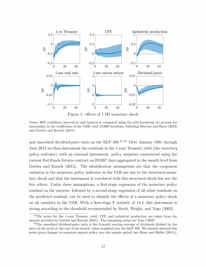
Figure 1: effects of 1 SD monetary shock
Notes: 90% confidence interval at each horizon is computed using the wild bootstrap (to account foruncertainty in the coefficients of the VAR) with 10,000 iterations, following Mertens and Ravn (2013)and Gertler and Karadi (2015).
and smoothed dividend-price ratio on the S&P 500.15,16 Over January 1991 through
June 2012 we then instrument the residuals in the 1-year Treasury yield (the monetary
policy indicator) with an external instrument: policy surprises constructed using the
current Fed Funds futures contract on FOMC days aggregated to the month level from
Gertler and Karadi (2015). The identification assumptions are that the exogenous
variation in the monetary policy indicator in the VAR are due to the structural mone-
tary shock and that the instrument is correlated with this structural shock but not the
five others. Under these assumptions, a first-stage regression of the monetary policy
residual on the surprise, followed by a second-stage regression of all other residuals on
the predicted residual, can be used to identify the effects of a monetary policy shock
on all variables in the VAR. With a first-stage F statistic of 14.4, this instrument is
strong according to the threshold recommended by Stock, Wright, and Yogo (2002).
15The series for the 1-year Treasury yield, CPI, and industrial production are taken from thedataset provided by Gertler and Karadi (2015). The remaining series are from CRSP.
16The smoothed dividend-price ratio is the 3-month moving average of dividends divided by theprice of the stock at the end of the month, value-weighted over the S&P 500. We linearly detrend thisseries given changes in corporate payout policy over the sample period (see Bunn and Shiller (2014)).
17
We then plot the impulse responses to a negative monetary policy shock using this
instrument in Figure 1. Since the structural monetary policy shock is not observed,
its magnitude should be interpreted through the lens of the approximately 0.2pp de-
crease in the 1-year yield on impact. Consistent with the wider literature, industrial
production and the price level rise, and the real interest rate falls. Excess returns rise
by 2pp on impact; given the comparatively tiny decline in the real interest rate, this
means the real return on the stock market is also approximately 2pp. Notably, excess
returns are small and negative in the months which follow, consistent with a decline in
the equity premium and the fall in the dividend/price ratio.
Following Bernanke and Kuttner (2005), we can decompose the 2pp real return on
the stock market into news about higher dividend growth, lower real risk-free discount
rates, and lower future excess returns using a Campbell-Shiller decomposition:
(real stock return)t − Et−1[(real stock return)t] = (Et − Et−1)∑j=0
κj∆(dividends)t+j
− (Et − Et−1)∑j=1
κj(real rate)t+j − (Et − Et−1)∑j=1
κj(excess return)t+j, (26)
where κ = 11+ d
p
and dp
is the steady-state dividend yield. Using the SVAR-IV to
compute the revised expectations in real rates and excess returns given the monetary
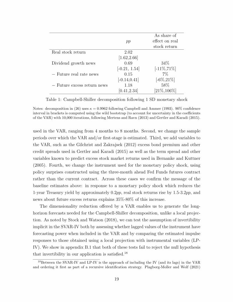
shock, we obtain the decomposition in Table 1.17 1.2pp (58%) of the initial return on
the stock market is due to news about lower future excess returns, 0.1pp (7%) is due to
news about lower future risk-free rates, and 0.7pp (34%) is due to news about higher
dividend growth. Accounting for estimation uncertainty, we conclude that at least 21%
and potentially all of the return on the stock market is due to news about lower future
excess returns, validating the original message from Bernanke and Kuttner (2005).
The important role of the risk premium in explaining the return on the stock market
is robust to details of the estimation approach. In appendix B.1 we modify the esti-
mation approach along a number of dimensions. First, we change the number of lags
17As in Bernanke and Kuttner (2005), we use our VAR to compute (excess return)t −Et−1[(excess return)t], (Et −Et−1)
∑j=1 κ
j(real rate)t+j , and (Et −Et−1)∑j=1 κ
j(excess return)t+j ,and we assign to dividend growth the residual implied by (26). As an alternative approach (availableon request), we use the estimated impulse responses for the dividend price ratio, real interest rate,and excess return to solve for the news about future dividend growth. The sum of terms on theright-hand side of (26) is slightly different from what the identity should imply, meaning that theestimated IRFs do not exactly satisfy this identity. However, we continue to find that news aboutfuture excess returns constitutes more than half of the sum of news from all three components.
18
ppAs share of
effect on realstock return
Real stock return 2.02[1.62,2.66]
Dividend growth news 0.69 34%[-0.21, 1.54] [-11%,71%]
− Future real rate news 0.15 7%[-0.14,0.41] [-6%,21%]
− Future excess return news 1.18 58%[0.41,2.34] [21%,106%]
Table 1: Campbell-Shiller decomposition following 1 SD monetary shock
Notes: decomposition in (26) uses κ = 0.9962 following Campbell and Ammer (1993). 90% confidenceinterval in brackets is computed using the wild bootstrap (to account for uncertainty in the coefficientsof the VAR) with 10,000 iterations, following Mertens and Ravn (2013) and Gertler and Karadi (2015).
used in the VAR, ranging from 4 months to 8 months. Second, we change the sample
periods over which the VAR and/or first-stage is estimated. Third, we add variables to
the VAR, such as the Gilchrist and Zakrajsek (2012) excess bond premium and other
credit spreads used in Gertler and Karadi (2015) as well as the term spread and other
variables known to predict excess stock market returns used in Bernanke and Kuttner
(2005). Fourth, we change the instrument used for the monetary policy shock, using
policy surprises constructed using the three-month ahead Fed Funds futures contract
rather than the current contract. Across these cases we confirm the message of the
baseline estimates above: in response to a monetary policy shock which reduces the
1-year Treasury yield by approximately 0.2pp, real stock returns rise by 1.5-3.2pp, and
news about future excess returns explains 35%-80% of this increase.
The dimensionality reduction offered by a VAR enables us to generate the long-
horizon forecasts needed for the Campbell-Shiller decomposition, unlike a local projec-
tion. As noted by Stock and Watson (2018), we can test the assumption of invertibility
implicit in the SVAR-IV both by assessing whether lagged values of the instrument have
forecasting power when included in the VAR and by comparing the estimated impulse
responses to those obtained using a local projection with instrumental variables (LP-
IV). We show in appendix B.1 that both of these tests fail to reject the null hypothesis
that invertibility in our application is satisfied.18
18Between the SVAR-IV and LP-IV is the approach of including the IV (and its lags) in the VARand ordering it first as part of a recursive identification strategy. Plagborg-Moller and Wolf (2021)
19
Finally, augmenting our VAR with cross-sectional data corroborates the redistribu-
tive mechanism through which our model rationalizes the risk premium response to a
monetary shock. In appendix B.1, we construct two measures of the relative wealth of
agents relatively more exposed to the stock market: a total return index of high beta
hedge funds relative to low beta hedge funds, and a total return index of high beta
mutual funds relative to low beta mutual funds. These measure the relative wealth of
a household continually (re-)invested in high beta funds relative to low beta funds. On
impact of a monetary easing, we find that the relative return of high beta funds rises
on impact and then falls thereafter — consistent with the wealth share of relatively
risk tolerant investors in our model, to which we now turn.
Objectives in the remainder of paper The rest of the paper enriches the model
from section 2 and studies a calibration to the U.S. economy matching micro evi-
dence on portfolio heterogeneity and conventional macro moments on asset prices and
business cycles. We first ask whether redistribution in such an environment can quan-
titatively rationalize the estimated stock market response to a monetary policy shock.
We then use the model to quantify the implications for the real economy.
3.2 Infinite horizon environment
We first outline the environment, building on that from section 2.1. We describe the
necessary changes here and present the complete environment in appendix C.
3.2.1 Household preferences and constraints
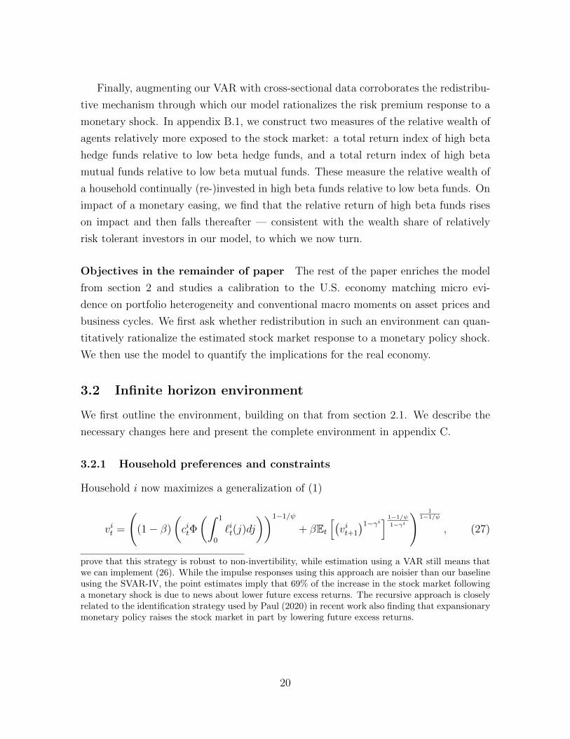
Household i now maximizes a generalization of (1)
vit =
((1− β)
(citΦ
(∫ 1
0
`it(j)dj
))1−1/ψ
+ βEt[(vit+1
)1−γi] 1−1/ψ
1−γi
) 11−1/ψ
, (27)
prove that this strategy is robust to non-invertibility, while estimation using a VAR still means thatwe can implement (26). While the impulse responses using this approach are noisier than our baselineusing the SVAR-IV, the point estimates imply that 69% of the increase in the stock market followinga monetary shock is due to news about lower future excess returns. The recursive approach is closelyrelated to the identification strategy used by Paul (2020) in recent work also finding that expansionarymonetary policy raises the stock market in part by lowering future excess returns.
20
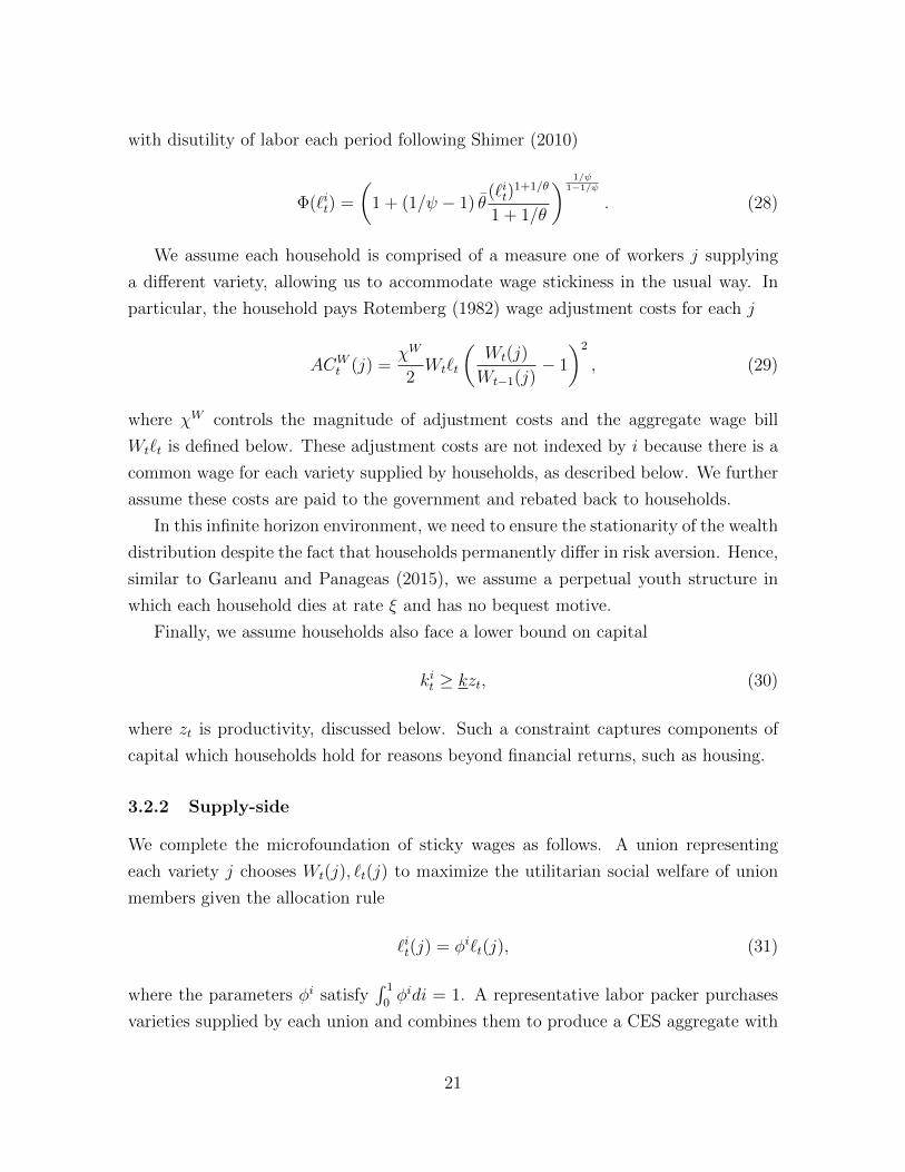
with disutility of labor each period following Shimer (2010)
Φ(`it) =
(1 + (1/ψ − 1) θ
(`it)1+1/θ
1 + 1/θ
) 1/ψ1−1/ψ
. (28)
We assume each household is comprised of a measure one of workers j supplying
a different variety, allowing us to accommodate wage stickiness in the usual way. In
particular, the household pays Rotemberg (1982) wage adjustment costs for each j
ACWt (j) =
χW
2Wt`t
(Wt(j)
Wt−1(j)− 1
)2
, (29)
where χW controls the magnitude of adjustment costs and the aggregate wage bill
Wt`t is defined below. These adjustment costs are not indexed by i because there is a
common wage for each variety supplied by households, as described below. We further
assume these costs are paid to the government and rebated back to households.
In this infinite horizon environment, we need to ensure the stationarity of the wealth
distribution despite the fact that households permanently differ in risk aversion. Hence,
similar to Garleanu and Panageas (2015), we assume a perpetual youth structure in
which each household dies at rate ξ and has no bequest motive.
Finally, we assume households also face a lower bound on capital
kit ≥ kzt, (30)
where zt is productivity, discussed below. Such a constraint captures components of
capital which households hold for reasons beyond financial returns, such as housing.
3.2.2 Supply-side
We complete the microfoundation of sticky wages as follows. A union representing
each variety j chooses Wt(j), `t(j) to maximize the utilitarian social welfare of union
members given the allocation rule
`it(j) = φi`t(j), (31)
where the parameters φi satisfy∫ 1
0φidi = 1. A representative labor packer purchases
varieties supplied by each union and combines them to produce a CES aggregate with
21
elasticity of substitution ε
`t =
[∫ 1
0
`t(j)(ε−1)/ε
]ε/(ε−1)(32)
which it then sells at Wt, earning
Wt`t −∫ 1
0
Wt(j)`t(j)dj. (33)
A representative producer then purchases the labor aggregate and rents capital, and it
uses consumption goods to produce new capital goods sold to households.
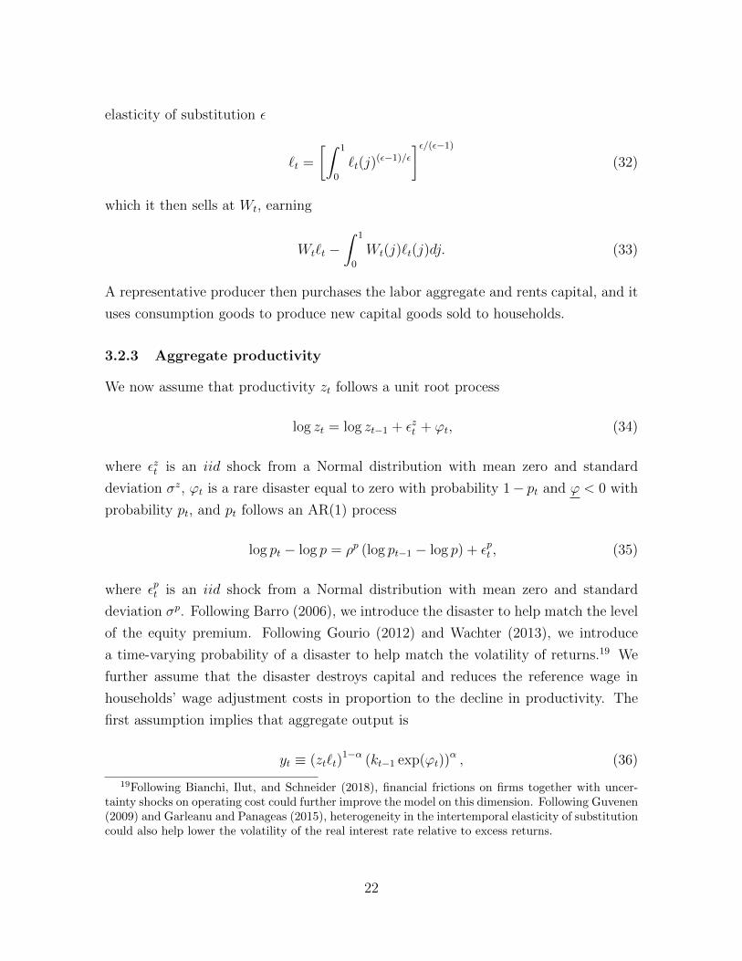
3.2.3 Aggregate productivity
We now assume that productivity zt follows a unit root process
log zt = log zt−1 + εzt + ϕt, (34)
where εzt is an iid shock from a Normal distribution with mean zero and standard
deviation σz, ϕt is a rare disaster equal to zero with probability 1− pt and ϕ < 0 with
probability pt, and pt follows an AR(1) process
log pt − log p = ρp (log pt−1 − log p) + εpt , (35)
where εpt is an iid shock from a Normal distribution with mean zero and standard
deviation σp. Following Barro (2006), we introduce the disaster to help match the level
of the equity premium. Following Gourio (2012) and Wachter (2013), we introduce
a time-varying probability of a disaster to help match the volatility of returns.19 We
further assume that the disaster destroys capital and reduces the reference wage in
households’ wage adjustment costs in proportion to the decline in productivity. The
first assumption implies that aggregate output is
yt ≡ (zt`t)1−α (kt−1 exp(ϕt))
α , (36)
19Following Bianchi, Ilut, and Schneider (2018), financial frictions on firms together with uncer-tainty shocks on operating cost could further improve the model on this dimension. Following Guvenen(2009) and Garleanu and Panageas (2015), heterogeneity in the intertemporal elasticity of substitutioncould also help lower the volatility of the real interest rate relative to excess returns.
22

where productivity is now labor-augmenting and thus consistent with balanced growth.
3.2.4 Monetary and fiscal policy
Finally, monetary policy is now characterized by the Taylor rule (8) each period
1 + it = (1 + i)
(PtPt−1
)φmt, (37)
where policy shocks follow an AR(1) process
logmt = ρm logmt−1 + εmt , (38)
where εmt is an iid shock from a Normal distribution with mean zero and standard
deviation σm.
Fiscal policy is characterized by three elements. First, the government subsidizes
workers’ labor income at a constant rate 1ε−1 rebated back to each household, eliminat-
ing the average wage markup in the usual way. Second, the government participates
in the bond market financed by lump-sum taxes in which household i pays a share
νi. Given the latter assumption (and that households face no constraints in the bond
market) the government bond position has no effect on the equilibrium allocation, so
we assume it is a constant real value relative to productivity: Bgt /(Ptzt) = bg. Its only
purpose is to make measured portfolios in model and data comparable. Third, the gov-
ernment collects the wealth of dying households and endows it to newborn households.
We describe the rule the government employs when doing so in the next subsection.
3.2.5 Equilibrium and model solution
The definition of equilibrium naturally generalizes Definition 1.
We solve the model globally using numerical methods. Given this, we limit the het-
erogeneity across households to make the computational burden tractable. We divide
the continuum of households into a finite number of groups within which households
have identical preferences. We choose three groups denoted i ∈ {a, b, c} where the
index i now refers to groups and the representative household of each group.20 The
20So that the model permits aggregation into representative households of each group despite theexistence of non-traded labor income, we allow households to trade claims to a labor endowment withother households in the same group, as further described in appendix C. This approach extends thatin Lenel (2020) to a setting with endogenous labor supply and production.
23
fraction of households belonging to group i is denoted λi, where∑
i λi = 1.
We solve a stationary transformation of the economy obtained by dividing all real
variables except labor by zt and nominal variables by Ptzt. In the transformed econ-
omy we obtain a recursive representation of the equilibrium in which the aggregate
state in period t is given by the monetary policy state variable mt, disaster proba-
bility pt, scaled aggregate capital kt−1/(zt−1 exp(εzt )), scaled prior period’s real wage
wt−1/(zt−1 exp(εzt )), and wealth shares {sit} of any two groups. Assuming that the gov-
ernment endows newborn households of each group with a share si of dying households’
wealth, these wealth shares follow
sit ≡ λi(1− ξ)(1 + it−1)(B
it−1 + νiBg
t−1) + (Πt + (1− δ)Qt)kit−1 exp(ϕt)
(Πt + (1− δ)Qt)kt−1 exp(ϕt)+ siξ. (39)
Productivity shocks inclusive of disasters only govern the transition across states, but
do not separately enter the state space itself.
We solve the model using sparse grids as described in Judd, Maliar, Maliar, and
Valero (2014). When forming expectations, we use Gauss-Hermite quadrature and
interpolate with Chebyshev polynomials for states off the grid. The stochastic equi-
librium is determined through backward iteration, while dampening the updating of
asset prices and individuals’ expectations over the dynamics of the aggregate states.
The code is written in Fortran and parallelized using OpenMP, so that convergence
can be achieved in a few minutes on a standard desktop computer.
3.3 Parameterization, first moments, and second moments
We now parameterize the model to match micro moments informing the heterogeneity
across groups as well as macro moments regarding the business cycle and asset prices.
3.3.1 Micro: the distribution of wealth, labor income, and portfolios
We seek to match the distribution of wealth, labor income, and financial portfolios in
U.S. data, giving us confidence in the model’s MPRs and exposures to a monetary
shock. We proceed in three steps with the 2016 Survey of Consumer Finances (SCF).
First, we decompose each household’s wealth (Ai) into claims on the economy’s
capital stock (Qki, in positive net supply) and nominal claims (Bi, in zero net supply
24
accounting for the government and rest of the world).21 We describe this procedure in
detail in appendix B.2 and provide a broad overview here. We first add estimates of
defined benefit pension wealth for each household since this is the major component
of household net worth which is excluded from the SCF.22 We then proceed by line
item to allocate how much household wealth is held in nominal claims versus claims
on capital.23,24 In the same spirit as Doepke and Schneider (2006), the key step in
doing this is to account for the implicit leverage households have on capital through
publicly-traded and privately-held businesses. In particular, if household i owns $1 in
equity in a firm which has net leverage
assets net of nominal assets
equity= lev,
then we assign the household Qki = lev and Bi = 1 − lev. The aggregate leverage
implicit in these equity claims must be consistent with that of the business sectors in
the Financial Accounts. We parameterize the dispersion in leverage in these claims to
match evidence on the dispersion in households’ expected rates of return.
Second, we stratify households by their wealth to labor income { Ai
W`i} and capital
portfolio share {QkiAi}, defining our three groups. We sort households on these variables
based on Proposition 5, which demonstrated that the capital portfolio share is infor-
mative about households’ risk aversion and thus MPR only after properly accounting
for their non-traded exposure to aggregate risk through labor income.25 Group a cor-
responds to households with high wealth to labor income and a high capital portfolio
share, group b corresponds to households with high wealth to labor income but a low
21Consistent with the traded assets in our model, we do not distinguish between nominal claimshaving different duration. In Kekre and Lenel (2021), we account for duration when calibrating amodel focused on the term premium.
22We use the estimates of Sabelhaus and Volz (2019) described further in the appendix. We thankJohn Sabelhaus for generously sharing their estimates with us.
23An alternative approach to measuring households’ portfolios would be to relate their changes inwealth to changes in asset prices using panel data, as in the recent work of Gomes (2019).
24We note in particular that we treat DB pension entitlements as a nominal asset of households,under the interpretation that households have a fixed claim on the pension sponsor which is then theresidual claimant on the investment portfolio. In contrast, DC pension assets, as with other mutualfund assets, are decomposed into nominal claims and claims on capital as described here.
25We sort households by a measure of their capital portfolio share after excluding from both thenumerator and denominator assets and liabilities associated with the primary residence and vehicles,even though for each group we report and target the capital portfolio share accounting for all assetsand liabilities. We sort households on the former measure since households’ decisions regarding theirprimary residence and consumer durables may reflect considerations beyond risk and return.
25
Ai
W`i
≥ p60 < p60
Qki
Ai
≥ p90
Group a
Share households: 4%∑i∈aW`i/
∑iW`i: 3% Group c∑
i∈aAi/∑
iAi: 18% Share households: 60%∑
i∈aQki/∑
i∈aAi: 2.0
∑i∈cW`i/
∑iW`i: 83%
< p90
Group b∑
i∈cAi/∑
iAi: 23%
Share households: 36%∑
i∈cQki/∑
i∈cAi: 1.1∑
i∈bW`i/∑
iW`i: 14%∑i∈bA
i/∑
iAi: 59%∑
i∈bQki/∑
i∈bAi: 0.5
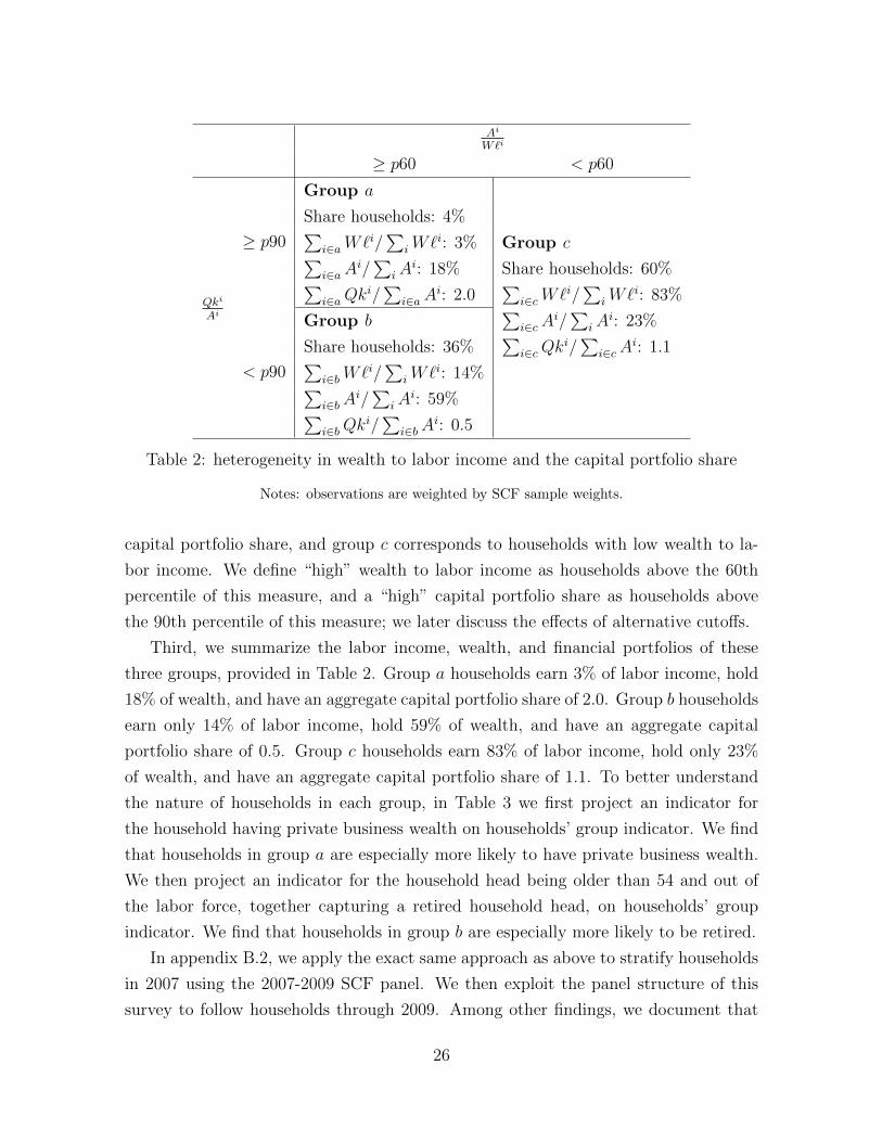
Table 2: heterogeneity in wealth to labor income and the capital portfolio share
Notes: observations are weighted by SCF sample weights.
capital portfolio share, and group c corresponds to households with low wealth to la-
bor income. We define “high” wealth to labor income as households above the 60th
percentile of this measure, and a “high” capital portfolio share as households above
the 90th percentile of this measure; we later discuss the effects of alternative cutoffs.
Third, we summarize the labor income, wealth, and financial portfolios of these
three groups, provided in Table 2. Group a households earn 3% of labor income, hold
18% of wealth, and have an aggregate capital portfolio share of 2.0. Group b households
earn only 14% of labor income, hold 59% of wealth, and have an aggregate capital
portfolio share of 0.5. Group c households earn 83% of labor income, hold only 23%
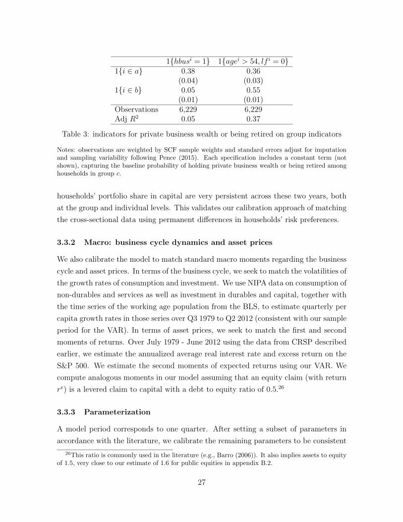
of wealth, and have an aggregate capital portfolio share of 1.1. To better understand
the nature of households in each group, in Table 3 we first project an indicator for
the household having private business wealth on households’ group indicator. We find
that households in group a are especially more likely to have private business wealth.
We then project an indicator for the household head being older than 54 and out of
the labor force, together capturing a retired household head, on households’ group
indicator. We find that households in group b are especially more likely to be retired.
In appendix B.2, we apply the exact same approach as above to stratify households
in 2007 using the 2007-2009 SCF panel. We then exploit the panel structure of this
survey to follow households through 2009. Among other findings, we document that
26
1{hbusi = 1} 1{agei > 54, lf i = 0}1{i ∈ a} 0.38 0.36
(0.04) (0.03)1{i ∈ b} 0.05 0.55
(0.01) (0.01)Observations 6,229 6,229Adj R2 0.05 0.37
Table 3: indicators for private business wealth or being retired on group indicators
Notes: observations are weighted by SCF sample weights and standard errors adjust for imputationand sampling variability following Pence (2015). Each specification includes a constant term (notshown), capturing the baseline probability of holding private business wealth or being retired amonghouseholds in group c.
households’ portfolio share in capital are very persistent across these two years, both
at the group and individual levels. This validates our calibration approach of matching
the cross-sectional data using permanent differences in households’ risk preferences.
3.3.2 Macro: business cycle dynamics and asset prices
We also calibrate the model to match standard macro moments regarding the business
cycle and asset prices. In terms of the business cycle, we seek to match the volatilities of
the growth rates of consumption and investment. We use NIPA data on consumption of
non-durables and services as well as investment in durables and capital, together with
the time series of the working age population from the BLS, to estimate quarterly per
capita growth rates in those series over Q3 1979 to Q2 2012 (consistent with our sample
period for the VAR). In terms of asset prices, we seek to match the first and second
moments of returns. Over July 1979 - June 2012 using the data from CRSP described
earlier, we estimate the annualized average real interest rate and excess return on the
S&P 500. We estimate the second moments of expected returns using our VAR. We
compute analogous moments in our model assuming that an equity claim (with return
re) is a levered claim to capital with a debt to equity ratio of 0.5.26
3.3.3 Parameterization
A model period corresponds to one quarter. After setting a subset of parameters in
accordance with the literature, we calibrate the remaining parameters to be consistent
26This ratio is commonly used in the literature (e.g., Barro (2006)). It also implies assets to equityof 1.5, very close to our estimate of 1.6 for public equities in appendix B.2.
27
with the macro and micro moments described above. All stochastic properties of the
model are estimated using a simulation where no disasters are realized in sample.27
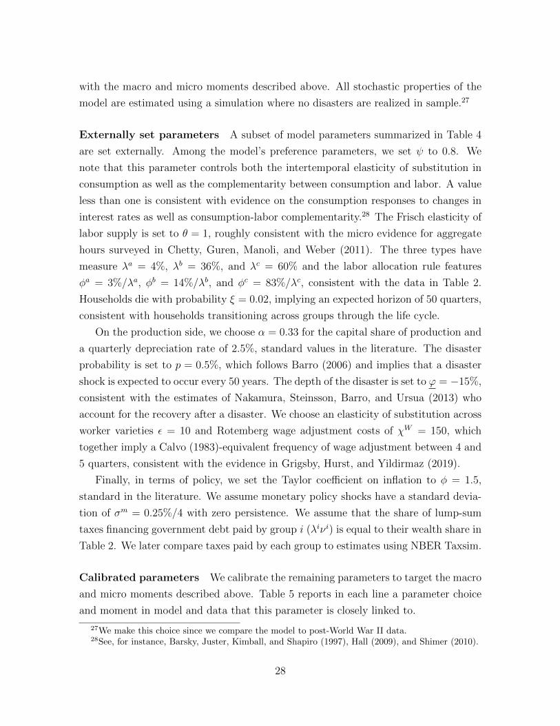
Externally set parameters A subset of model parameters summarized in Table 4
are set externally. Among the model’s preference parameters, we set ψ to 0.8. We
note that this parameter controls both the intertemporal elasticity of substitution in
consumption as well as the complementarity between consumption and labor. A value
less than one is consistent with evidence on the consumption responses to changes in
interest rates as well as consumption-labor complementarity.28 The Frisch elasticity of
labor supply is set to θ = 1, roughly consistent with the micro evidence for aggregate
hours surveyed in Chetty, Guren, Manoli, and Weber (2011). The three types have
measure λa = 4%, λb = 36%, and λc = 60% and the labor allocation rule features
φa = 3%/λa, φb = 14%/λb, and φc = 83%/λc, consistent with the data in Table 2.
Households die with probability ξ = 0.02, implying an expected horizon of 50 quarters,
consistent with households transitioning across groups through the life cycle.
On the production side, we choose α = 0.33 for the capital share of production and
a quarterly depreciation rate of 2.5%, standard values in the literature. The disaster
probability is set to p = 0.5%, which follows Barro (2006) and implies that a disaster
shock is expected to occur every 50 years. The depth of the disaster is set to ϕ = −15%,
consistent with the estimates of Nakamura, Steinsson, Barro, and Ursua (2013) who
account for the recovery after a disaster. We choose an elasticity of substitution across
worker varieties ε = 10 and Rotemberg wage adjustment costs of χW = 150, which
together imply a Calvo (1983)-equivalent frequency of wage adjustment between 4 and
5 quarters, consistent with the evidence in Grigsby, Hurst, and Yildirmaz (2019).
Finally, in terms of policy, we set the Taylor coefficient on inflation to φ = 1.5,
standard in the literature. We assume monetary policy shocks have a standard devia-
tion of σm = 0.25%/4 with zero persistence. We assume that the share of lump-sum
taxes financing government debt paid by group i (λiνi) is equal to their wealth share in
Table 2. We later compare taxes paid by each group to estimates using NBER Taxsim.
Calibrated parameters We calibrate the remaining parameters to target the macro
and micro moments described above. Table 5 reports in each line a parameter choice
and moment in model and data that this parameter is closely linked to.
27We make this choice since we compare the model to post-World War II data.28See, for instance, Barsky, Juster, Kimball, and Shapiro (1997), Hall (2009), and Shimer (2010).
28
Description Value Notes
ψ IES 0.8
θ Frisch elasticity 1 Chetty et al. (2011)
λa measure of a households 4% population in SCF
λb measure of b households 36% population in SCF
φa labor a households 3%/λa labor income in SCF
φb labor b households 14%/λb labor income in SCF
ξ death probability 0.02
α 1 - labor share 0.33
δ depreciation rate 2.5%
ε elast. of subs. across workers 10
χW Rotemberg wage adj costs 150 ≈ P(adjust) = 4− 5 qtrs
p disaster probability 0.5% Barro (2006)
ϕ disaster shock -15% Nakamura et al. (2013)
φ Taylor coeff. on inflation 1.5 Taylor (1993)
σm std. dev. MP shock 0.25%/4
ρm persistence MP shock 0
λaνa a share of taxes to finance −Bg 18% wealth in SCF
λbνb b share of taxes to finance −Bg 59% wealth in SCF
Table 4: externally set parameters
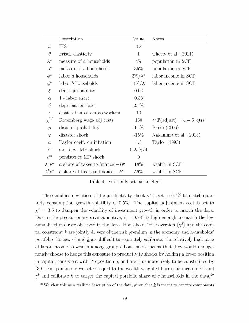
The standard deviation of the productivity shock σz is set to 0.7% to match quar-
terly consumption growth volatility of 0.5%. The capital adjustment cost is set to
χx = 3.5 to dampen the volatility of investment growth in order to match the data.
Due to the precautionary savings motive, β = 0.987 is high enough to match the low
annualized real rate observed in the data. Households’ risk aversion {γi} and the capi-
tal constraint k are jointly drivers of the risk premium in the economy and households’
portfolio choices. γc and k are difficult to separately calibrate: the relatively high ratio
of labor income to wealth among group c households means that they would endoge-
nously choose to hedge this exposure to productivity shocks by holding a lower position
in capital, consistent with Proposition 5, and are thus more likely to be constrained by
(30). For parsimony we set γc equal to the wealth-weighted harmonic mean of γa and
γb and calibrate k to target the capital portfolio share of c households in the data,29
29We view this as a realistic description of the data, given that k is meant to capture components
29
Description Value Moment Target Model
σz std. dev. prod. 0.7% σ(∆ log c) 0.5% 0.6%
χx capital adj cost 3.5 σ(∆ log x) 2.1% 2.1%
β discount factor 0.987 4Er+1 1.4% 1.5%
γb RRA b 26 4E[re+1 − r+1
]7.1% 7.1%
σp variation log dis. prob. 0.47 σ (4Er+1) 2.3% 2.1%
ρp persist. log dis. prob. 0.80 ρ(4Er+1) 0.80 0.76
γa RRA a 10 ka/aa 2.0 2.3
k lower bound ki 0.4k kc/ac 1.1 1.0
sa newborn endowment a 0% λaaa/∑
i λiai 18% 21%
sc newborn endowment c 40% λcac/∑
i λici 23% 21%
bg real value govt bonds -3.1 −∑
i λibi/
∑i λ
iai -11% -11%
Table 5: targeted moments and calibrated parameters
Notes: targeted business cycle moments are from Q3/79-Q2/12 NIPA and targeted asset pricingmoments are from 7/79-6/12 data underlying the VAR. The model assumes a debt/equity ratio of 0.5on a stock market claim. The first and second moments in the model are estimated over 50,000 quartersafter a burn-in period of 5,000 quarters, with no disaster realizations in sample. The disutilities oflabor {θa, θb, θc} are jointly set to {0.73, 3.24, 0.44} so that the average labor wedge is zero for eachgroup and ` = 1, where the latter is a convenient normalization.
obtaining k set to 0.4 times the average capital holdings of households in the model.
The variation σp and persistence ρp in the disaster probability are chosen to target the
standard deviation and autocorrelation of the annualized expected real interest rate
from our VAR. The initial endowments of newborns are chosen to target the measured
wealth shares of the three groups. We set bg so that on average, the aggregate bond
position of households relative to total wealth is 11%, as in the SCF data underlying
Table 2. Finally we set the disutilities of labor for each group so that the average labor
wedge is zero for each group and ` = 1, the latter being a convenient normalization.
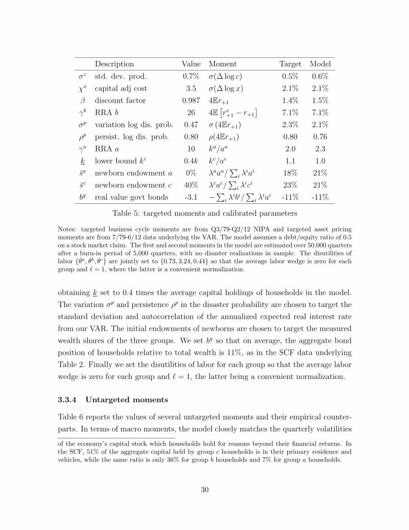
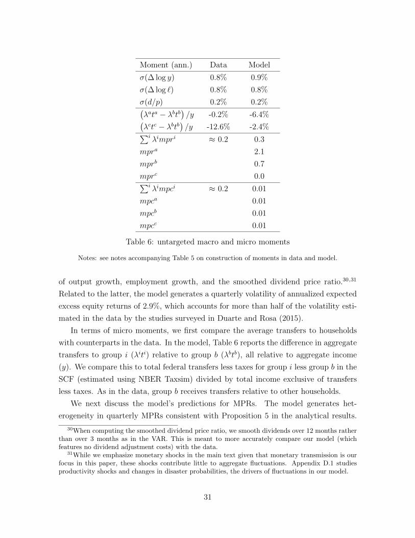
3.3.4 Untargeted moments
Table 6 reports the values of several untargeted moments and their empirical counter-
parts. In terms of macro moments, the model closely matches the quarterly volatilities
of the economy’s capital stock which households hold for reasons beyond their financial returns. Inthe SCF, 51% of the aggregate capital held by group c households is in their primary residence andvehicles, while the same ratio is only 36% for group b households and 7% for group a households.
30
Moment (ann.) Data Model
σ(∆ log y) 0.8% 0.9%
σ(∆ log `) 0.8% 0.8%
σ(d/p) 0.2% 0.2%(λata − λbtb
)/y -0.2% -6.4%(
λctc − λbtb)/y -12.6% -2.4%∑i λimpri ≈ 0.2 0.3
mpra 2.1
mprb 0.7
mprc 0.0∑i λimpci ≈ 0.2 0.01
mpca 0.01
mpcb 0.01
mpcc 0.01
Table 6: untargeted macro and micro moments
Notes: see notes accompanying Table 5 on construction of moments in data and model.
of output growth, employment growth, and the smoothed dividend price ratio.30,31
Related to the latter, the model generates a quarterly volatility of annualized expected
excess equity returns of 2.9%, which accounts for more than half of the volatility esti-
mated in the data by the studies surveyed in Duarte and Rosa (2015).
In terms of micro moments, we first compare the average transfers to households
with counterparts in the data. In the model, Table 6 reports the difference in aggregate
transfers to group i (λiti) relative to group b (λbtb), all relative to aggregate income
(y). We compare this to total federal transfers less taxes for group i less group b in the
SCF (estimated using NBER Taxsim) divided by total income exclusive of transfers
less taxes. As in the data, group b receives transfers relative to other households.
We next discuss the model’s predictions for MPRs. The model generates het-
erogeneity in quarterly MPRs consistent with Proposition 5 in the analytical results.
30When computing the smoothed dividend price ratio, we smooth dividends over 12 months ratherthan over 3 months as in the VAR. This is meant to more accurately compare our model (whichfeatures no dividend adjustment costs) with the data.
31While we emphasize monetary shocks in the main text given that monetary transmission is ourfocus in this paper, these shocks contribute little to aggregate fluctuations. Appendix D.1 studiesproductivity shocks and changes in disaster probabilities, the drivers of fluctuations in our model.
31
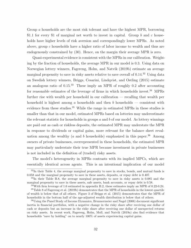
Group a households are the most risk tolerant and have the highest MPR, borrowing
$1.1 for every $1 of marginal net worth to invest in capital. Group b and c house-
holds have higher levels of risk aversion and correspondingly lower MPRs. As noted
above, group c households have a higher ratio of labor income to wealth and thus are
endogenously constrained by (30). Hence, on the margin their average MPR is zero.
Quasi-experimental evidence is consistent with the MPRs in our calibration. Weight-
ing by the fraction of households, the average MPR in our model is 0.3. Using data on
Norwegian lottery winners, Fagereng, Holm, and Natvik (2019b) estimate an average
marginal propensity to save in risky assets relative to save overall of 0.14.32 Using data
on Swedish lottery winners, Briggs, Cesarini, Lindqvist, and Ostling (2015) estimate
an analogous ratio of 0.15.33 These imply an MPR of roughly 0.2 after accounting
for reasonable estimates of the leverage of firms in which households invest.34 MPRs
further rise with wealth per household in our calibration — recalling that wealth per
household is highest among a households and then b households — consistent with
evidence from these studies.35 While the range in estimated MPRs in these studies is
smaller than that in our model, estimated MPRs based on lotteries may underestimate
the relevant statistic for households in groups a and b of our model. As lottery winnings
are paid out as cash or riskless deposits, the estimated MPR may understate the MPR
in response to dividends or capital gains, more relevant for the balance sheet reval-
uation among the wealthy (a and b households) emphasized in this paper.36 Among
owners of private businesses, overrepresented in these households, the estimated MPR
may particularly understate their true MPR because investment in private businesses
is not included in the definition of (traded) risky assets.
The model’s heterogeneity in MPRs contrasts with its implied MPCs, which are
essentially identical across agents. This is an intentional implication of our model
32In their Table 4, the average marginal propensity to save in stocks, bonds, and mutual funds is0.058 and the marginal propensity to save in these assets, deposits, or repay debt is 0.407.
33In their Table B.8, the average marginal propensity to save in risky assets is 0.085 and themarginal propensity to save in these assets, safe assets, bank accounts, or repay debt is 0.58.
34With firm leverage of 1.6 estimated in appendix B.2, these estimates imply an MPR of 0.22-0.24.35Table 8 of Fagereng et al. (2019b) demonstrates that the MPR of households in the lowest quartile
of wealth is below that of all others. Figure 3 of Briggs et al. (2015) demonstrates that the MPR ofhouseholds in the bottom half of the age-adjusted wealth distribution is below that of others.
36Using the Panel Study of Income Dynamics, Brunnermeier and Nagel (2008) document significantinertia in financial portfolios, with a negative change in the risky share after receiving one dollar ofcash or deposits but an increase in the risky share after receiving one dollar of unexpected returnson risky assets. In recent work, Fagereng, Holm, Moll, and Natvik (2019a) also find evidence thathouseholds “save by holding” on to nearly 100% of assets experiencing capital gains.
32
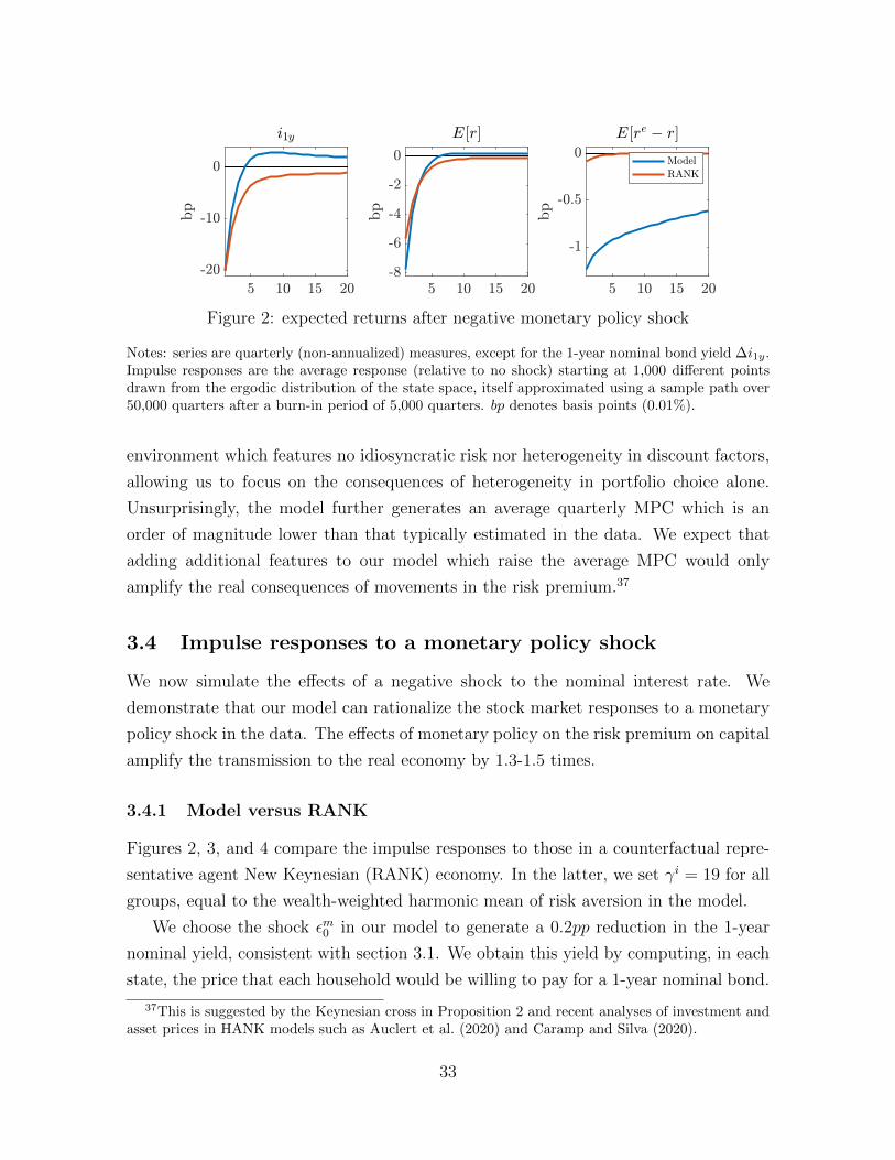
Figure 2: expected returns after negative monetary policy shock
Notes: series are quarterly (non-annualized) measures, except for the 1-year nominal bond yield ∆i1y.Impulse responses are the average response (relative to no shock) starting at 1,000 different pointsdrawn from the ergodic distribution of the state space, itself approximated using a sample path over50,000 quarters after a burn-in period of 5,000 quarters. bp denotes basis points (0.01%).
environment which features no idiosyncratic risk nor heterogeneity in discount factors,
allowing us to focus on the consequences of heterogeneity in portfolio choice alone.
Unsurprisingly, the model further generates an average quarterly MPC which is an
order of magnitude lower than that typically estimated in the data. We expect that
adding additional features to our model which raise the average MPC would only
amplify the real consequences of movements in the risk premium.37
3.4 Impulse responses to a monetary policy shock
We now simulate the effects of a negative shock to the nominal interest rate. We
demonstrate that our model can rationalize the stock market responses to a monetary
policy shock in the data. The effects of monetary policy on the risk premium on capital
amplify the transmission to the real economy by 1.3-1.5 times.
3.4.1 Model versus RANK
Figures 2, 3, and 4 compare the impulse responses to those in a counterfactual repre-
sentative agent New Keynesian (RANK) economy. In the latter, we set γi = 19 for all
groups, equal to the wealth-weighted harmonic mean of risk aversion in the model.
We choose the shock εm0 in our model to generate a 0.2pp reduction in the 1-year
nominal yield, consistent with section 3.1. We obtain this yield by computing, in each
state, the price that each household would be willing to pay for a 1-year nominal bond.
37This is suggested by the Keynesian cross in Proposition 2 and recent analyses of investment andasset prices in HANK models such as Auclert et al. (2020) and Caramp and Silva (2020).
33
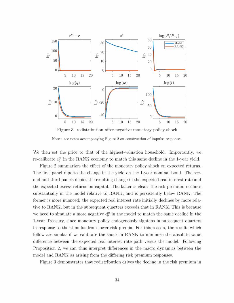
Figure 3: redistribution after negative monetary policy shock
Notes: see notes accompanying Figure 2 on construction of impulse responses.
We then set the price to that of the highest-valuation household. Importantly, we
re-calibrate εm0 in the RANK economy to match this same decline in the 1-year yield.
Figure 2 summarizes the effect of the monetary policy shock on expected returns.
The first panel reports the change in the yield on the 1-year nominal bond. The sec-
ond and third panels depict the resulting change in the expected real interest rate and
the expected excess returns on capital. The latter is clear: the risk premium declines
substantially in the model relative to RANK, and is persistently below RANK. The
former is more nuanced: the expected real interest rate initially declines by more rela-
tive to RANK, but in the subsequent quarters exceeds that in RANK. This is because
we need to simulate a more negative εm0 in the model to match the same decline in the
1-year Treasury, since monetary policy endogenously tightens in subsequent quarters
in response to the stimulus from lower risk premia. For this reason, the results which
follow are similar if we calibrate the shock in RANK to minimize the absolute value
difference between the expected real interest rate path versus the model. Following
Proposition 2, we can thus interpret differences in the macro dynamics between the
model and RANK as arising from the differing risk premium responses.
Figure 3 demonstrates that redistribution drives the decline in the risk premium in
34
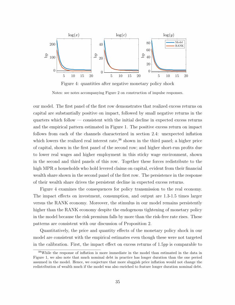
Figure 4: quantities after negative monetary policy shock
Notes: see notes accompanying Figure 2 on construction of impulse responses.
our model. The first panel of the first row demonstrates that realized excess returns on
capital are substantially positive on impact, followed by small negative returns in the
quarters which follow — consistent with the initial decline in expected excess returns
and the empirical pattern estimated in Figure 1. The positive excess return on impact
follows from each of the channels characterized in section 2.4: unexpected inflation
which lowers the realized real interest rate,38 shown in the third panel; a higher price
of capital, shown in the first panel of the second row; and higher short-run profits due
to lower real wages and higher employment in this sticky wage environment, shown
in the second and third panels of this row. Together these forces redistribute to the
high MPR a households who hold levered claims on capital, evident from their financial
wealth share shown in the second panel of the first row. The persistence in the response
of their wealth share drives the persistent decline in expected excess returns.
Figure 4 examines the consequences for policy transmission to the real economy.
The impact effects on investment, consumption, and output are 1.3-1.5 times larger
versus the RANK economy. Moreover, the stimulus in our model remains persistently
higher than the RANK economy despite the endogenous tightening of monetary policy
in the model because the risk premium falls by more than the risk-free rate rises. These
patterns are consistent with our discussion of Proposition 2.
Quantitatively, the price and quantity effects of the monetary policy shock in our
model are consistent with the empirical estimates even though these were not targeted
in the calibration. First, the impact effect on excess returns of 1.5pp is comparable to
38While the response of inflation is more immediate in the model than estimated in the data inFigure 1, we also note that much nominal debt in practice has longer duration than the one periodassumed in the model. Hence, we conjecture that more sluggish price inflation would not change theredistribution of wealth much if the model was also enriched to feature longer duration nominal debt.
35
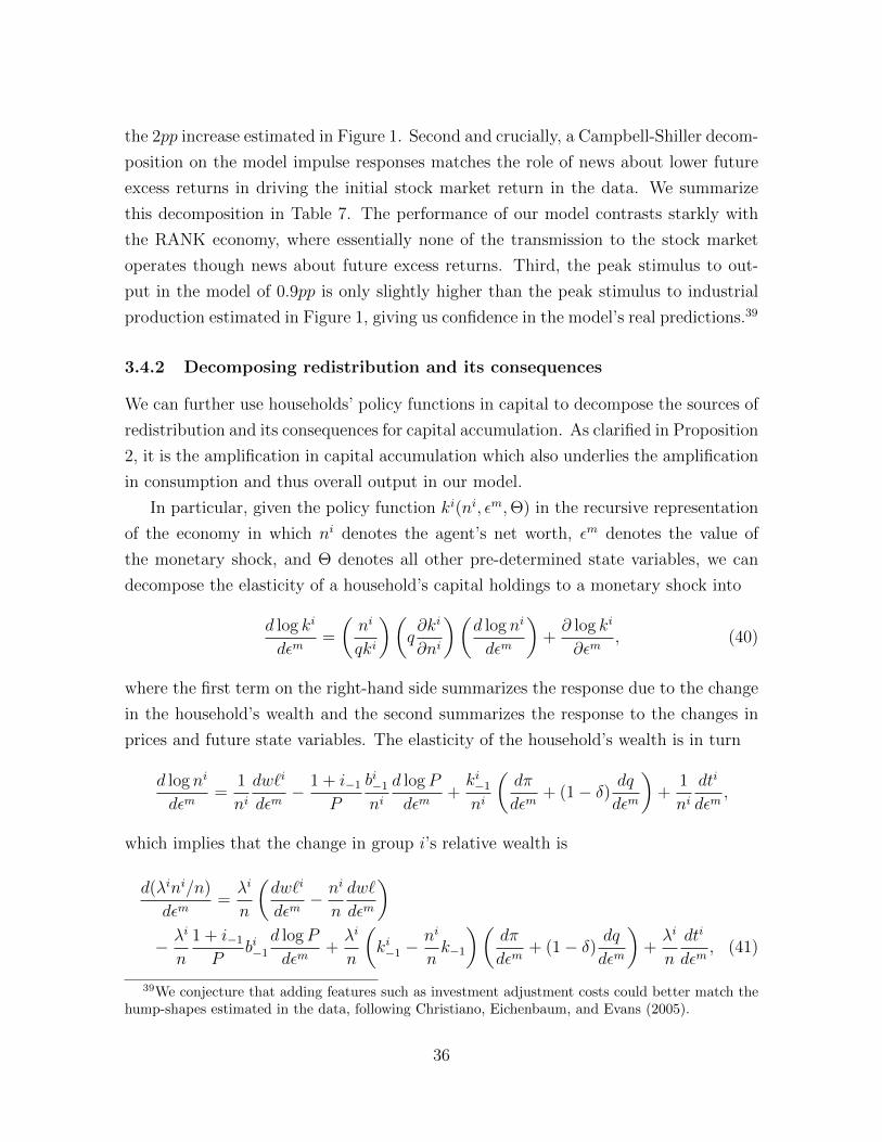
the 2pp increase estimated in Figure 1. Second and crucially, a Campbell-Shiller decom-
position on the model impulse responses matches the role of news about lower future
excess returns in driving the initial stock market return in the data. We summarize
this decomposition in Table 7. The performance of our model contrasts starkly with
the RANK economy, where essentially none of the transmission to the stock market
operates though news about future excess returns. Third, the peak stimulus to out-
put in the model of 0.9pp is only slightly higher than the peak stimulus to industrial
production estimated in Figure 1, giving us confidence in the model’s real predictions.39
3.4.2 Decomposing redistribution and its consequences
We can further use households’ policy functions in capital to decompose the sources of
redistribution and its consequences for capital accumulation. As clarified in Proposition
2, it is the amplification in capital accumulation which also underlies the amplification
in consumption and thus overall output in our model.
In particular, given the policy function ki(ni, εm,Θ) in the recursive representation
of the economy in which ni denotes the agent’s net worth, εm denotes the value of
the monetary shock, and Θ denotes all other pre-determined state variables, we can
decompose the elasticity of a household’s capital holdings to a monetary shock into
d log ki
dεm=
(ni
qki
)(q∂ki
∂ni
)(d log ni
dεm
)+∂ log ki
∂εm, (40)
where the first term on the right-hand side summarizes the response due to the change
in the household’s wealth and the second summarizes the response to the changes in
prices and future state variables. The elasticity of the household’s wealth is in turn
d log ni
dεm=
1
nidw`i
dεm− 1 + i−1
P
bi−1ni
d logP
dεm+ki−1ni
(dπ
dεm+ (1− δ) dq
dεm
)+
1
nidti
dεm,
which implies that the change in group i’s relative wealth is
d(λini/n)
dεm=λi
n
(dw`i
dεm− ni
n
dw`
dεm
)− λi
n
1 + i−1P
bi−1d logP
dεm+λi
n
(ki−1 −
ni
nk−1
)(dπ
dεm+ (1− δ) dq
dεm
)+λi
n
dti
dεm, (41)
39We conjecture that adding features such as investment adjustment costs could better match thehump-shapes estimated in the data, following Christiano, Eichenbaum, and Evans (2005).
36
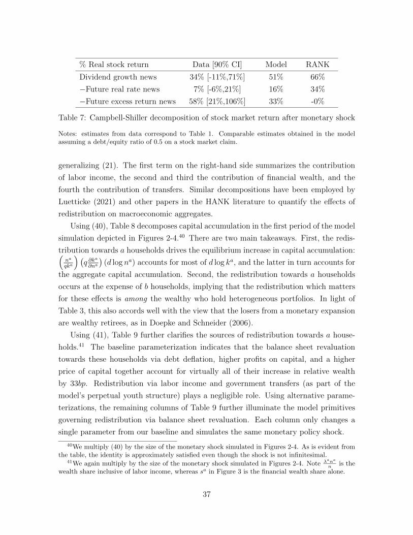
% Real stock return Data [90% CI] Model RANK
Dividend growth news 34% [-11%,71%] 51% 66%
−Future real rate news 7% [-6%,21%] 16% 34%
−Future excess return news 58% [21%,106%] 33% -0%
Table 7: Campbell-Shiller decomposition of stock market return after monetary shock
Notes: estimates from data correspond to Table 1. Comparable estimates obtained in the modelassuming a debt/equity ratio of 0.5 on a stock market claim.
generalizing (21). The first term on the right-hand side summarizes the contribution
of labor income, the second and third the contribution of financial wealth, and the
fourth the contribution of transfers. Similar decompositions have been employed by
Luetticke (2021) and other papers in the HANK literature to quantify the effects of
redistribution on macroeconomic aggregates.
Using (40), Table 8 decomposes capital accumulation in the first period of the model
simulation depicted in Figures 2-4.40 There are two main takeaways. First, the redis-
tribution towards a households drives the equilibrium increase in capital accumulation:(na
qka
) (q ∂k
a
∂na
)(d log na) accounts for most of d log ka, and the latter in turn accounts for
the aggregate capital accumulation. Second, the redistribution towards a households
occurs at the expense of b households, implying that the redistribution which matters
for these effects is among the wealthy who hold heterogeneous portfolios. In light of
Table 3, this also accords well with the view that the losers from a monetary expansion
are wealthy retirees, as in Doepke and Schneider (2006).
Using (41), Table 9 further clarifies the sources of redistribution towards a house-
holds.41 The baseline parameterization indicates that the balance sheet revaluation
towards these households via debt deflation, higher profits on capital, and a higher
price of capital together account for virtually all of their increase in relative wealth
by 33bp. Redistribution via labor income and government transfers (as part of the
model’s perpetual youth structure) plays a negligible role. Using alternative parame-
terizations, the remaining columns of Table 9 further illuminate the model primitives
governing redistribution via balance sheet revaluation. Each column only changes a
single parameter from our baseline and simulates the same monetary policy shock.
40We multiply (40) by the size of the monetary shock simulated in Figures 2-4. As is evident fromthe table, the identity is approximately satisfied even though the shock is not infinitesimal.
41We again multiply by the size of the monetary shock simulated in Figures 2-4. Note λana
n is thewealth share inclusive of labor income, whereas sa in Figure 3 is the financial wealth share alone.
37
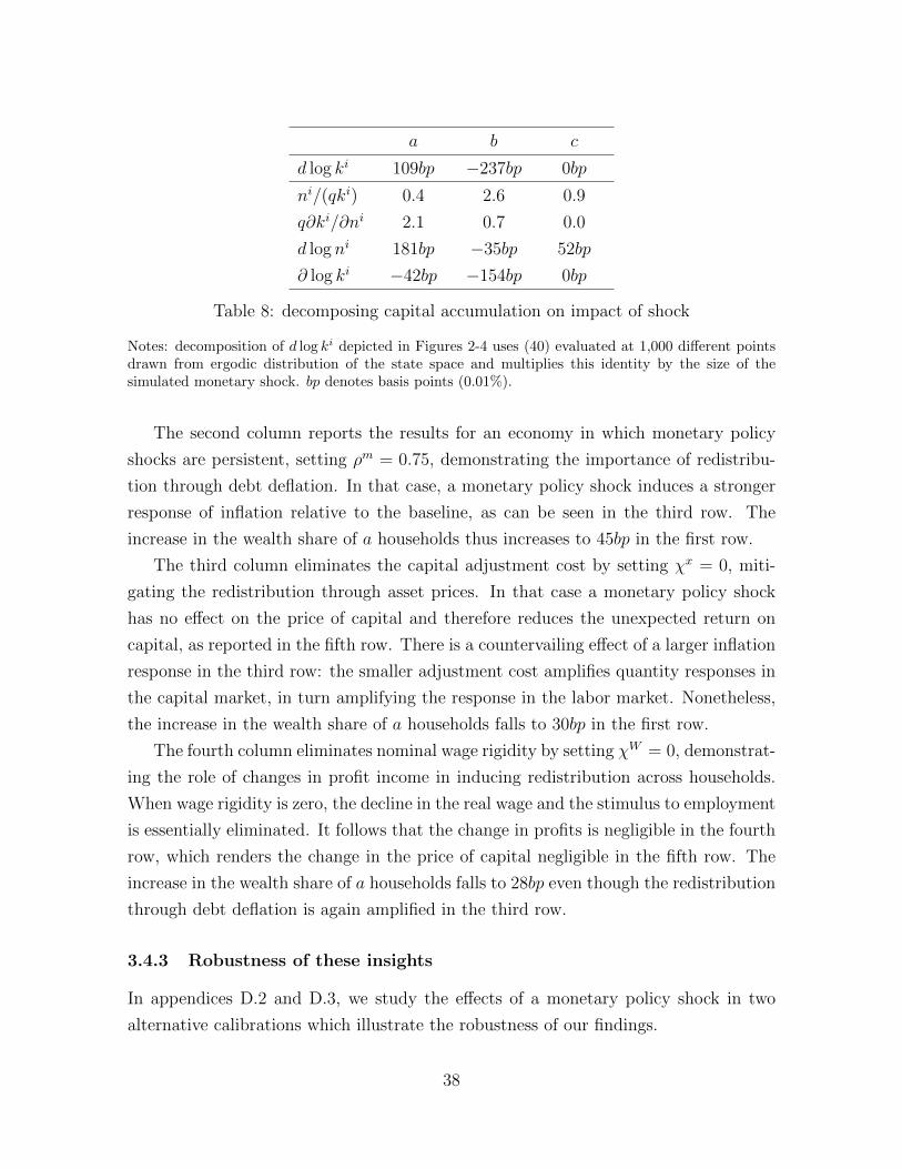
a b c
d log ki 109bp −237bp 0bp
ni/(qki) 0.4 2.6 0.9
q∂ki/∂ni 2.1 0.7 0.0
d log ni 181bp −35bp 52bp
∂ log ki −42bp −154bp 0bp
Table 8: decomposing capital accumulation on impact of shock
Notes: decomposition of d log ki depicted in Figures 2-4 uses (40) evaluated at 1,000 different pointsdrawn from ergodic distribution of the state space and multiplies this identity by the size of thesimulated monetary shock. bp denotes basis points (0.01%).
The second column reports the results for an economy in which monetary policy
shocks are persistent, setting ρm = 0.75, demonstrating the importance of redistribu-
tion through debt deflation. In that case, a monetary policy shock induces a stronger
response of inflation relative to the baseline, as can be seen in the third row. The
increase in the wealth share of a households thus increases to 45bp in the first row.
The third column eliminates the capital adjustment cost by setting χx = 0, miti-
gating the redistribution through asset prices. In that case a monetary policy shock
has no effect on the price of capital and therefore reduces the unexpected return on
capital, as reported in the fifth row. There is a countervailing effect of a larger inflation
response in the third row: the smaller adjustment cost amplifies quantity responses in
the capital market, in turn amplifying the response in the labor market. Nonetheless,
the increase in the wealth share of a households falls to 30bp in the first row.
The fourth column eliminates nominal wage rigidity by setting χW = 0, demonstrat-
ing the role of changes in profit income in inducing redistribution across households.
When wage rigidity is zero, the decline in the real wage and the stimulus to employment
is essentially eliminated. It follows that the change in profits is negligible in the fourth
row, which renders the change in the price of capital negligible in the fifth row. The
increase in the wealth share of a households falls to 28bp even though the redistribution
through debt deflation is again amplified in the third row.
3.4.3 Robustness of these insights
In appendices D.2 and D.3, we study the effects of a monetary policy shock in two
alternative calibrations which illustrate the robustness of our findings.
38
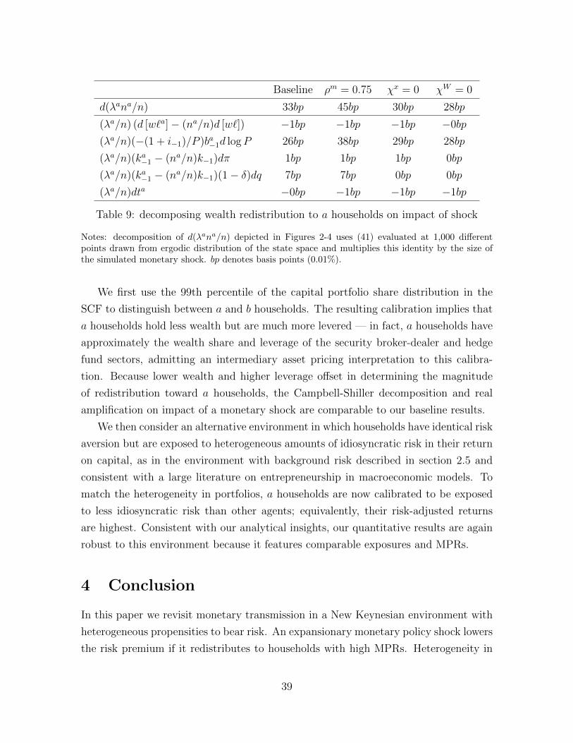
Baseline ρm = 0.75 χx = 0 χW = 0
d(λana/n) 33bp 45bp 30bp 28bp
(λa/n) (d [w`a]− (na/n)d [w`]) −1bp −1bp −1bp −0bp
(λa/n)(−(1 + i−1)/P )ba−1d logP 26bp 38bp 29bp 28bp
(λa/n)(ka−1 − (na/n)k−1)dπ 1bp 1bp 1bp 0bp
(λa/n)(ka−1 − (na/n)k−1)(1− δ)dq 7bp 7bp 0bp 0bp
(λa/n)dta −0bp −1bp −1bp −1bp
Table 9: decomposing wealth redistribution to a households on impact of shock
Notes: decomposition of d(λana/n) depicted in Figures 2-4 uses (41) evaluated at 1,000 differentpoints drawn from ergodic distribution of the state space and multiplies this identity by the size ofthe simulated monetary shock. bp denotes basis points (0.01%).
We first use the 99th percentile of the capital portfolio share distribution in the
SCF to distinguish between a and b households. The resulting calibration implies that
a households hold less wealth but are much more levered — in fact, a households have
approximately the wealth share and leverage of the security broker-dealer and hedge
fund sectors, admitting an intermediary asset pricing interpretation to this calibra-
tion. Because lower wealth and higher leverage offset in determining the magnitude
of redistribution toward a households, the Campbell-Shiller decomposition and real
amplification on impact of a monetary shock are comparable to our baseline results.
We then consider an alternative environment in which households have identical risk
aversion but are exposed to heterogeneous amounts of idiosyncratic risk in their return
on capital, as in the environment with background risk described in section 2.5 and
consistent with a large literature on entrepreneurship in macroeconomic models. To
match the heterogeneity in portfolios, a households are now calibrated to be exposed
to less idiosyncratic risk than other agents; equivalently, their risk-adjusted returns
are highest. Consistent with our analytical insights, our quantitative results are again
robust to this environment because it features comparable exposures and MPRs.
4 Conclusion
In this paper we revisit monetary transmission in a New Keynesian environment with
heterogeneous propensities to bear risk. An expansionary monetary policy shock lowers
the risk premium if it redistributes to households with high MPRs. Heterogeneity in
39
risk aversion, portfolio constraints, rules of thumb, background risk, or beliefs imply
redistribution in this way. In a calibration matching heterogeneity in the U.S. economy,
this mechanism rationalizes the stock market effects of monetary policy which have
eluded existing frameworks and amplifies its transmission to the real economy.
The framework of this paper can be further developed along a number of dimensions.
First, it seems fruitful to synthesize our perspective emphasizing assets’ exposure to
aggregate risk with the existing HANK literature emphasizing asset liquidity: in such
a setting, an investor’s MPR out of liquid versus illiquid wealth will differ, likely a
better match to the micro data. Second, while we have focused for concreteness on
the equity premium, a natural question is the extent to which our insights can explain
the broader effects of monetary policy across asset classes, as in the Treasury market
or foreign exchange market. Third, while our analysis has focused on the conditional
responses to monetary policy shocks, it would be useful to examine the model’s implied
comovements when featuring a richer set of business cycle shocks calibrated to the data.
We leave these questions for future work.
References
Alvarez, F., A. Atkeson, and P. J. Kehoe (2009): “Time-varying risk, interestrates, and exchange rates in general equilibrium,” Review of Economic Studies, 76,851–878.
Alves, F., G. Kaplan, B. Moll, and G. L. Violante (2020): “A further lookat the propagation of monetary policy shocks in HANK,” Journal of Money, Creditand Banking, 52, 521–559.
Auclert, A. (2019): “Monetary policy and the redistribution channel,” AmericanEconomic Review, 109, 2333–2367.
Auclert, A., M. Rognlie, and L. Straub (2020): “Micro jumps, macro humps:monetary policy and business cycles in an estimated HANK model,” Working paper.
Barro, R. J. (2006): “Rare disasters and asset markets in the twentieth century,”Quarterly Journal of Economics, 121, 823–866.
Barsky, R. B., F. T. Juster, M. S. Kimball, and M. D. Shapiro (1997):“Preference parameters and behavioral heterogeneity: an experimental approach inthe Health and Retirement Study,” Quarterly Journal of Economics, 112, 537–579.
40

Basu, S. and B. Bundick (2017): “Uncertainty shocks in a model of effective de-mand,” Econometrica, 85, 937–958.
Bernanke, B. S., M. Gertler, and S. Gilchrist (1999): The financial accel-erator in a quantitative business cycle framework, Elsevier, vol. 1 of Handbook ofMacroeconomics, 1341–1393.
Bernanke, B. S. and K. N. Kuttner (2005): “What explains the stock market’sreaction to Federal Reserve policy?” Journal of Finance, 60, 1221–1257.
Bhandari, A., D. Evans, and M. Golosov (2019): “Risk and asset prices in amonetary model,” Working paper.
Bianchi, F., C. Ilut, and M. Schneider (2018): “Uncertainty shocks, asset supplyand pricing over the business cycle,” Review of Economic Studies, 85, 810–854.
Bianchi, F., M. Lettau, and S. C. Ludvigson (2021): “Monetary policy andasset valuation,” Journal of Finance, forthcoming.
Briggs, J., D. Cesarini, E. Lindqvist, and R. Ostling (2015): “Wealth, port-folio allocations, and risk preference,” Working paper.
Brunnermeier, M. and Y. Sannikov (2012): “Redistributive monetary policy,”Proceedings of the Symposium at Jackson Hole.
Brunnermeier, M. K. and S. Nagel (2008): “Do wealth fluctuations generatetime-varying risk aversion? Micro-evidence on individuals’ asset allocation,” Amer-ican Economic Review, 98, 713–736.
Brunnermeier, M. K. and Y. Sannikov (2014): “A macroeconomic model witha financial sector,” American Economic Review, 104, 379–421.
——— (2016): “The I theory of money,” Working paper.
Bunn, O. D. and R. J. Shiller (2014): “Changing times, changing values: ahistorical analysis of sectors within the U.S. stock market 1872-2013,” Working paper.
Caballero, R. and E. Farhi (2018): “The safety trap,” Review of Economic Stud-ies, 85, 223–274.
Caballero, R. and A. Simsek (2020): “A risk-centric model of demand recessionsand speculation,” Quarterly Journal of Economics, 135, 1493–1566.
Calvo, G. A. (1983): “Staggered prices in a utility-maximizing framework,” Journalof Monetary Economics, 12, 383–398.
Campbell, J. Y. and J. Ammer (1993): “What moves the stock and bond markets?A variance decomposition for long-term asset returns,” Journal of Finance, 48, 3–37.
41
Campbell, J. Y. and R. J. Shiller (1988): “The dividend-price ratio and expec-tations of future dividends and discount factors,” Review of Financial Studies, 1,195–228.
Caramp, N. and D. H. Silva (2020): “Monetary policy and wealth effects: the roleof risk and heterogeneity,” Working paper.
Chen, W. and G. Phelan (2019): “Dynamic consequences of monetary policy forfinancial stability,” Working paper.
Chetty, R., A. Guren, D. Manoli, and A. Weber (2011): “Are micro andmacro labor supply elasticities consistent? A review of evidence on the intensive andextensive margins,” American Economic Review, 101, 471–475.
Chien, Y., H. Cole, and H. Lustig (2012): “Is the volatility of the market priceof risk due to intermittent portfolio rebalancing?” American Economic Review, 106,2859–2896.
Chodorow-Reich, G., P. T. Nenov, and A. Simsek (2020): “Stock marketwealth and the real economy: a local labor market approach,” American EconomicReview.
Christiano, L. J., M. Eichenbaum, and C. L. Evans (2005): “Nominal rigiditiesand the dynamic effects of a shock to monetary policy,” Journal of Political Economy,113, 1–45.
Coimbra, N. and H. Rey (2020): “Financial cycles with heterogeneous intermedi-aries,” Working paper.
Constantinides, G. M. and D. Duffie (1996): “Asset pricing with heterogeneousconsumers,” Journal of Political Economy, 104, 219–240.
Devereux, M. B. and A. Sutherland (2011): “Country portfolios in open econ-omy macro-models,” Journal of the European Economic Association, 9, 337–369.
DiTella, S. (2020): “Risk premia and the real effects of money,” American EconomicReview, 110, 1995–2040.
Doepke, M. and M. Schneider (2006): “Inflation and the redistribution of nominalwealth,” Journal of Political Economy, 114, 1069–1097.
Drechsler, I., A. Savov, and P. Schnabl (2018): “A model of monetary policyand risk premia,” Journal of Finance, 63, 317–373.
Duarte, F. and C. Rosa (2015): “The equity risk premium: a review of models,”FRBNY Economic Policy Review.
42
Epstein, L. G. and S. E. Zin (1991): “Substitution, risk aversion, and the temporalbehavior of consumption and asset returns: an empirical analysis,” Econometrica,99, 263–286.
Fagereng, A., M. B. Holm, B. Moll, and G. Natvik (2019a): “Saving behavioracross the wealth distribution: the importance of capital gains,” Working paper.
Fagereng, A., M. B. Holm, and G. J. Natvik (2019b): “MPC heterogeneity andhousehold balance sheets,” Working paper.
Fernandez-Villaverde, J., P. Guerron-Quintana, K. Kuester, andJ. Rubio-Ramirez (2015): “Fiscal volatility shocks and economic activity,” Amer-ican Economic Review, 105, 3352–3384.
Gali, J. (2008): Monetary policy, inflation, and the business cycle, Princeton Univer-sity Press.
Garleanu, N. and S. Panageas (2015): “Young, Old, Conservative, and Bold. Theimplications of finite lives and heterogeneity for asset pricing,” Journal of PoliticalEconomy, 123, 670–685.
Geanakoplos, J. (2009): “The leverage cycle,” NBER Macroeconomics Annual, 24.
Gertler, M. and P. Karadi (2015): “Monetary policy surprises, credit costs, andeconomic activity,” American Economic Journal: Macroeconomics, 7, 44–76.
Gilchrist, S. and E. Zakrajsek (2012): “Credit spreads and business cycle fluc-tuations,” American Economic Review, 102, 1692–1720.
Gomes, M. (2019): “Asset prices and wealth inequality,” Working paper.
Gourio, F. (2012): “Disaster Risk and Business Cycles,” American Economic Review,102, 2734–2766.
Grigsby, J., E. Hurst, and A. Yildirmaz (2019): “Aggregate nominal wageadjustments: new evidence from administrative payroll data,” Working paper.
Guvenen, F. (2009): “A parsimonious macroeconomic model for asset pricing,”Econometrica, 77, 1711–1750.
Hall, R. E. (2009): “Reconciling cyclical movements in the marginal value of timeand the marginal product of labor,” Journal of Political Economy, 117, 281–323.
Hanson, S. G. and J. C. Stein (2015): “Monetary policy and long-term real rates,”Journal of Financial Economics, 115, 429–448.
He, Z. and A. Krishnamurthy (2013): “Intermediary Asset Pricing,” AmericanEconomic Review, 2, 732–770.
43
Ilut, C. L. and M. Schneider (2014): “Ambiguous business cycles,” AmericanEconomic Review, 104, 2368–2399.
Jarocinski, M. and P. Karadi (2020): “Deconstructing monetary policy surprises– the role of information shocks,” American Economic Journal: Macroeconomics,12, 1–43.
Judd, K. L., L. Maliar, S. Maliar, and R. Valero (2014): “Smolyak methodsfor solving dynamic economic models: Lagrange interpolation, anistropic grid andadaptive domain,” Journal of Economic Dynamics and Control, 44, 92–123.
Kaplan, G., B. Moll, and G. L. Violante (2018): “Monetary policy accordingto HANK,” American Economic Review, 108, 697–743.
Kaplan, G. and G. L. Violante (2018): “Microeconomic heterogeneity andmacroeconomic shocks,” Journal of Economic Perspectives.
Kekre, R. and M. Lenel (2021): “Heterogeneity, monetary policy, and the termpremium,” Working paper.
Krueger, D. and H. Lustig (2010): “When is market incompleteness irrelevant forthe price of aggregate risk (and when is it not)?” Journal of Economic Theory, 145,1–41.
Lenel, M. (2020): “Safe assets, collateralized lending and monetary policy,” Workingpaper.
Lopez-Salido, D., J. C. Stein, and E. Zakrajsek (2017): “Credit-market sen-timent and the business cycle,” Quarterly Journal of Economics, 132, 1373–1426.
Luetticke, R. (2021): “Transmission of monetary policy with heterogeneity in house-hold portfolios,” American Economic Journal: Macroeconomics, 13, 1–25.
Melcangi, D. and V. Sterk (2021): “Stock market participation, inequality, andmonetary policy,” Working paper.
Mertens, K. and M. O. Ravn (2013): “The dynamic effects of personal and cor-porate income tax changes in the United States,” American Economic Review, 103,1212–1247.
Nakamura, E. and J. Steinsson (2018): “High frequency identification of mone-tary non-neutrality: the information effect,” Quarterly Journal of Economics, 133,1283–1330.
Nakamura, E., J. Steinsson, R. Barro, and J. Ursua (2013): “Crises andrecoveries in an empirical model of consumption disasters,” American EconomicJournal: Macroeconomics, 5, 35–74.
44
Panageas, S. (2020): “The implications of heterogeneity and inequality for assetpricing,” Foundations and Trends in Finance, 15, forthcoming.
Paul, P. (2020): “The time-varying effect of monetary policy on asset prices,” Reviewof Economics and Statistics, 102, 690–704.
Pence, K. (2015): “SCFCOMBO: Stata module to estimate errors using the Surveyof Consumer Finances,” Tech. rep., Boston College Department of Economics.
Pflueger, C. and G. Rinaldi (2021): “Why does the Fed move markets so much?A model of monetary policy and time-varying risk aversion,” Working paper.
Pflueger, C., E. Siriwardane, and A. Sunderam (2020): “Financial market riskperceptions and the macroeconomy,” Quarterly Journal of Economics, 135, 1443–1491.
Plagborg-Moller, M. and C. K. Wolf (2021): “Local projections and VARsestimate the same impulse responses,” Econometrica, 89, 955–980.
Rotemberg, J. J. (1982): “Sticky prices in the United States,” Journal of PoliticalEconomy, 90, 1187–1211.
Sabelhaus, J. and A. H. Volz (2019): “Are disappearing employer pensions con-tributing to rising wealth inequality?” Working paper.
Shimer, R. (2010): Labor markets and business cycles, Princeton University Press.
Stock, J. H. and M. W. Watson (2018): “Identification and estimation of dy-namic causal effects in macroeconomics using external instruments,” The EconomicJournal, 128, 917–948.
Stock, J. H., J. H. Wright, and M. Yogo (2002): “A survey of weak instrumentsand weak identification in generalized method of moments,” Journal of Business andEconomic Statistics, 20, 518–529.
Taylor, J. B. (1993): “Discretion Versus Policy Rules in Practice,” Carnegie-Rochester Conference Series on Public Policy, 39, 195–214.
Toda, A. A. and K. J. Walsh (2020): “The equity premium and the one percent,”Review of Financial Studies, 33, 3583–3623.
Wachter, J. A. (2013): “Can time-varying risk of rare disasters explain aggregatestock market volatility,” Journal of Finance, 68, 987–1035.
Woodford, M. (2003): Interest and prices: foundations of a theory of monetarypolicy, Princeton University Press.
45

Online AppendixMonetary Policy, Redistribution, and Risk Premia
A Proofs of analytical results
A.1 Proposition 1
Proof. Multiplying both sides of (14) by ai0, integrating over all i, and then using asset
market clearing∫ 1
0ai0ω
i0di =
∫ 1
0ai0di, we obtain the claimed expression for the risk
premium on capital. Differentiating with respect to εm0 , we have that
d[E0 log(1 + rk1)− log(1 + r1)
]dεm0
= σ2 dγ
dεm0= γσ2
∫ 1
0
d[ai0/∫ 1
0ai′
0 di′]
dεm0
(1− ωi0
)di,
as claimed, where the second equality uses (14) and asset market clearing.
A.2 Proposition 2
Proof. The result for dk0dεm0
follows from differentiating (16). Now differentiating house-
hold i’s consumption policy function and (17) and integrating over all i yields
dc0
dεm0= (1− β)
[dy0
dεm0+
(1− δ0)q0k−1
k0
χxdk0
dεm0
],
where we have used firms’ flow of funds, asset market clearing, and equilibrium invest-
ment. Differentiating goods market clearing and using equilibrium investment yields
dy0
dεm0=dc0
dεm0+ q0
(1 +
x0
k0
χx)dk0
dεm0.
Combining these and using capital accumulation yields the result for dc0dεm0
.
A.3 Proposition 3
Proof. The Taylor rule and Fisher equation imply
dπP0dεm0
=1
φ
d log(1 + r1)
dεm0− 1
φ. (A.1)
A1

Combining with equilibrium labor demand, the production function, and a rigid nom-
inal wage in period 0 yields
1
y0
dy0
dεm0=
1− αα
1
φ
d log(1 + r1)
dεm0− 1− α
α
1
φ. (A.2)
By (15), (18), and (20), it follows that
dk0
dεm0= − k0
1− α + χx
[−γσ2 1
n0
Covi(dni0dεm0
, ωi0
)+d log(1 + r1)
dεm0
], (A.3)
where Covi denotes a cross-sectional covariance. Combining this with (21), (A.1),
1
π0
dπ0
dεm0=
1
y0
dy0
dεm0(A.4)
implied by equilibrium profits, and
1
q0
dq0
dεm0= χx
1
k0
dk0
dεm0(A.5)
implied by equilibrium investment, we have that
Covi(dni0dεm0
, ωi0
)=
1
1− γσ2(1− δ0) q0n0
χx
1−α+χxCovi(ki−1, ω
i0)×[
− Covi(
1 + i−1
P0
Bi−1, ω
i0
)(1
φ
d log(1 + r1)
dεm0− 1
φ
)+(
π0
y0
dy0
dεm0− (1− δ0)q0
χx
1 + α + χxd log(1 + r1)
dεm0
)Covi
(ki−1, ω
i0
) ]. (A.6)
Finally, combining (A.3) and (19) yields
dy0
dεm0=
[γσ2Covi
(dni0dεm0
, ωi0
)− n0
d log(1 + r1)
dεm0
]×(
1 + χx (1− β(1− δ0)k−1/k0)
1− α + χx
). (A.7)
With heterogeneity in γi and the assumption that households’ initial endowments
are consistent with the portfolios (14), we have Covi(Bi−1, ω
i0
)< 0 and Covi
(ki−1, ω
i0
)>
0. At least around the RANK benchmark with the same aggregate allocation, the sys-
A2

tem of equations (A.2), (A.6), and (A.7) thus implies
dy0
dεm0<dy0
dεm0|RANK < 0,
Covi(dni0dεm0
, ωi0
)< 0 = Covi
(dni0dεm0
, ωi0
)|RANK ,
0 <d log(1 + r1)
dεm0<d log(1 + r1)
dεm0|RANK < 1.
We can thus conclude from (A.1), (A.4), and (A.5) that a monetary tightening gen-
erates deflation, a fall in profits, and a fall in the price of capital; from (A.6) that it
generates a rise in the risk premium only in the model with heterogeneity; and that
the real effects of a monetary shock are amplified in the model with heterogeneity.
A.4 Proposition 4
Proof. For a household up against a portfolio constraint or following a rule-of-thumb,
their equilibrium portfolio ωi0 is simply implied by the constraint or rule-of-thumb. For
all other households, a Taylor approximation of (13) yields the optimal portfolio share
in capital
ωi0 ≈1
γi(ς i + ηi)
Ei0 log(1 + rk,i1 )− log(1 + r1) + 12(ς i + ηi)σ2
σ2, (A.8)
where Ei0 is the household’s subjective expectation and rk,i1 is the return on capital
accounting for the idiosyncratic component of its return. Given the distributional
assumptions on ηi and ς i, we have that
Ei0 log(1 + rk,i1 )− log(1 + r1) +1
2(ς i + ηi)σ2 = E0 log(1 + rk1)− log(1 + r1) +
1
2σ2, (A.9)
where E0 denotes the objective expectation and rk1 the return on capital without id-
iosyncratic risk (equivalently, aggregating over idiosyncratic risk). Then multiplying
both sides of (A.8) by ai0, integrating over all unconstrained households which we de-
note as the set i /∈ C, and then using asset market clearing, it is straightforward to
show
E0 log(1 + rk1)− log(1 + r1) +1
2σ2 = γσ2
A3

where now
γ ≡
(1−
∫i/∈C a
i0(1− ωi0)di∫i/∈C a
i0di
)(∫i/∈C
ai0∫i′ /∈C a
i′0 di′
1
γi(ς i + ηi)di
)−1
.
Differentiating and again using market clearing, (A.8) for unconstrained households,
and (A.9) yields
d[E0 log(1 + rk1)− log(1 + r1)
]dεm0
= γ
( ∫ 1
0ai0di∫
i/∈C ai0ω
i0di
)σ2
∫ 1
0
d[ai0/∫ 1
0ai′
0 di′]
dεm0
(1− ωi0
)di.
The remaining arguments in Propositions 2 and 3 are unchanged.
A.5 Proposition 5
Proof. We first characterize households’ portfolio share in capital in the limit of zero
aggregate risk. Up to second-order, (13) implies
E0rk1 − r1 +
1
2σ2 = γiδc
i1z1σ2 + o(|| · ||3) (A.10)
given the first-order approximation of ci1 in terms of the states
ci1 = δci1z1εz1 + δc
i1m0εm0 + o(|| · ||2)
with coefficients δ··. Anticipating the result in Proposition 1, it follows that
δci1z1
=γ
γi. (A.11)
Approximating up to first order the period 1 resource constraint and equilibrium wages
and profits, the method of undetermined coefficients implies
δci1z1
=w1 + π1k
i0
ci1. (A.12)
Substituting in (A.11) and re-arranging, we can conclude that
q0ki0
ai0=
π1ki0
(1 + r1)ai0=
ci1(1 + r1)ai0
γ
γi− w1
(1 + r1)ai0,
A4

where the first equality uses q0 = π11+r1
absent aggregate risk.
We now characterize households’ marginal responses to a unit of income in the limit
of zero aggregate risk. Differentiating and combining households’ optimal portfolio
choice condition and period 1 resource constraint yields
0 = E0
(ci1)−γi γi
ci1(rk1 − r1)
((1 + r1)
∂bi0∂ni0
+ π1∂ki0∂ni0
). (A.13)
A second-order approximation then implies
0 =
((1 + r1)
∂bi0∂ni0
+ π1∂ki0∂ni0
)(E0r
k1 − r1 +
1
2σ2
)
−
((1 + r1)
∂bi0∂ni0
+ π1∂ki0∂ni0
)γi + 1
ci1
(w1 + π1k
i0
)σ2 + π1
∂ki0∂ni0
σ2 + o(|| · ||3). (A.14)
Again anticipating the result in Proposition 1 and using (A.11) and (A.12), it follows
from (A.14) that
q0∂ki0∂ni0
=γ
γi∂ai0∂ni0
using q0 = π11+r0
and∂bi0∂ni0
+ q0∂ki0∂ni0
=∂ai0∂ni0
. The expression for mpri0 ≡q0∂ki0∂ni0
∂ai0∂ni0
follows.
A.6 Proposition 6
Proof. We first derive the result up to second order. Multiplying both sides of (A.10) byci1γi
, integrating over all households i, and making use of the market clearing conditions
which imply that ∫ 1
0
ci1di =
∫ 1
0
(w1 + π1k
i0
)di,
we obtain
E0rk1 − r0 +
1
2σ2 =
(ci1∫ 1
0ci′
1 di′
1
γi
)−1
σ2 + o(|| · ||3), (A.15)
defining γ as in the claim.
We now derive the result up to third order. The third-order approximation of
optimal portfolio choice for household i is
A5

E0rk1 − r1 +
1
2σ2 =
γiδci1z1σ2 +
[γi(δci1m0γ + δc
i1m0z1
)−(γi)2δci1m0δci1z1
+ γiδci1z1δr1m0− γδr1m0
]εm0 σ
2 + o(|| · ||4).
given the second-order expansion of ci1 in terms of the underlying states
ci1 = δci1m0εm0 + δc
i1z1εz1 +
1
2δci1m2
0(εm0 )2 + δc
i1m0z1
εm0 εz1 +
1
2δci1z21
(εz1)2 +1
2δci1σ2σ
2 + o(|| · ||3).
Making use of (A.11) substantially simplifies this to
E0rk1 − r1 +
1
2σ2 = γiδc
i1z1σ2 + γiδc
i1m0z1
εm0 σ2 + o(|| · ||4). (A.16)
Again multiplying both sides byci1γi
, integrating over all households i, and making use
of the market clearing conditions, we obtain
E0rk1 − r1 +
1
2σ2 = γσ2 +
γ∫ 1
0ci1di
(∫ 1
0
ci1δci1m0z1
di
)εm0 σ
2 + o(|| · ||4).
It remains to further characterize the coefficient on εm0 σ2 in closed form. Taking a
second-order approximation of the period 1 resource constraint and equilibrium wages
and profits, the method of undetermined coefficients implies
ci1δci1m0z1
+ ci1δci1m0δci1z1
= αw1δk0m0
+ π1δki0m0− (1− α)π1k
i0δk0m0. (A.17)
It follows that ∫ 1
0
ci1δci1m0z1
di = −∫ 1
0
ci1δci1m0δci1z1di+ π1
∫ 1
0
δki0m0di,
using market clearing and the definition of equilibrium wages and profits.1 Further
using a first-order approximation to capital claims market clearing and goods market
clearing implies∫ 1
0
ci1δci1m0z1
di =
∫ 1
0
ci1δci1m0
(1− δci1z1
)di =
∫ 1
0
ci1δci1m0
(1− γ
γi
)di,
where the second equality uses (A.11). Recall from Proposition 5 that mpri0 ≡γγi
.
1We linearize rather than log-linearize with respect to {ki0, bi0, ai0} since these may be negative.
A6
Since the definition of γ implies
∫ 1
0
ci1δci1m0
(1− γ
γi
)di =
∫ 1
0
(ci1δ
ci1m0− ci1∫ 1
0ci′
1 di′
∫ 1
0
ci′
1 δci′1m0di′
)(1− γ
γi
)di
and
d[ci1/∫ 1
0ci′
1
]dεm0
=1∫ 1
0ci′
1 di′
(ci1δ
ci1m0− ci1∫ 1
0ci′
1 di′
∫ 1
0
ci′
1 δci′1m0di′
),
we obtain the coefficient on εm0 σ2 given in the claim.
B Empirical appendix
B.1 The effect of monetary shocks
B.1.1 Robustness to details of estimation approach
We first demonstrate that the broad messages of our baseline estimates of the effects
of a monetary policy shock in section 3.1 are robust to details of the estimation.
Given a monetary policy shock, Table A.1 summarizes the impact effect on the
1-year Treasury yield, the impact effect on the real S&P 500 return (implied by the
real rate and excess return), and the share of the latter accounted for by news about
future excess returns in the Campbell-Shiller decomposition (26). First, we find that
the baseline results using 6 lags in the VAR are little affected if 4-8 lags are used
instead. Second, we find that the results are broadly robust to using the same January
1991 - June 2012 period for both the VAR and IV regressions, or limiting the analysis
of monetary policy shocks to the first half of the IV sample alone (January 1991 -
September 2001). The expansionary monetary policy shock lowers the stock market
when using the second half of the IV sample alone (October 2001 - June 2012), but we
note that the instrument is weak over this sub-sample (having a first-stage F statistic
of 4.7, not shown). Third, we find that news about future excess returns tends to be,
if anything, even more important when adding other variables included in the analyses
of Bernanke and Kuttner (2005) and Gertler and Karadi (2015) on which we build.
Finally, we find similar results when using as the instrument the three-month ahead
Fed Funds futures contract instead of the current contract.
A7
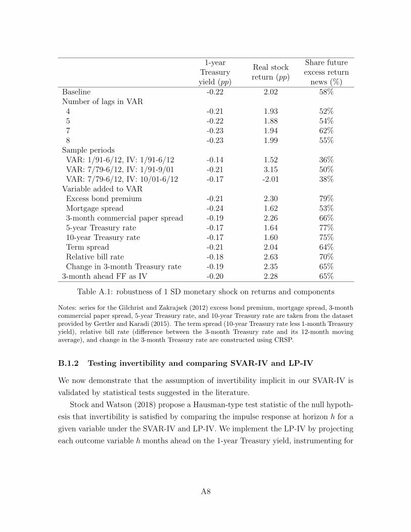
1-yearTreasuryyield (pp)
Real stockreturn (pp)
Share futureexcess return
news (%)Baseline -0.22 2.02 58%Number of lags in VAR4 -0.21 1.93 52%5 -0.22 1.88 54%7 -0.23 1.94 62%8 -0.23 1.99 55%
Sample periodsVAR: 1/91-6/12, IV: 1/91-6/12 -0.14 1.52 36%VAR: 7/79-6/12, IV: 1/91-9/01 -0.21 3.15 50%VAR: 7/79-6/12, IV: 10/01-6/12 -0.17 -2.01 38%
Variable added to VARExcess bond premium -0.21 2.30 79%Mortgage spread -0.24 1.62 53%3-month commercial paper spread -0.19 2.26 66%5-year Treasury rate -0.17 1.64 77%10-year Treasury rate -0.17 1.60 75%Term spread -0.21 2.04 64%Relative bill rate -0.18 2.63 70%Change in 3-month Treasury rate -0.19 2.35 65%
3-month ahead FF as IV -0.20 2.28 65%
Table A.1: robustness of 1 SD monetary shock on returns and components
Notes: series for the Gilchrist and Zakrajsek (2012) excess bond premium, mortgage spread, 3-monthcommercial paper spread, 5-year Treasury rate, and 10-year Treasury rate are taken from the datasetprovided by Gertler and Karadi (2015). The term spread (10-year Treasury rate less 1-month Treasuryyield), relative bill rate (difference between the 3-month Treasury rate and its 12-month movingaverage), and change in the 3-month Treasury rate are constructed using CRSP.
B.1.2 Testing invertibility and comparing SVAR-IV and LP-IV
We now demonstrate that the assumption of invertibility implicit in our SVAR-IV is
validated by statistical tests suggested in the literature.
Stock and Watson (2018) propose a Hausman-type test statistic of the null hypoth-
esis that invertibility is satisfied by comparing the impulse response at horizon h for a
given variable under the SVAR-IV and LP-IV. We implement the LP-IV by projecting
each outcome variable h months ahead on the 1-year Treasury yield, instrumenting for
A8
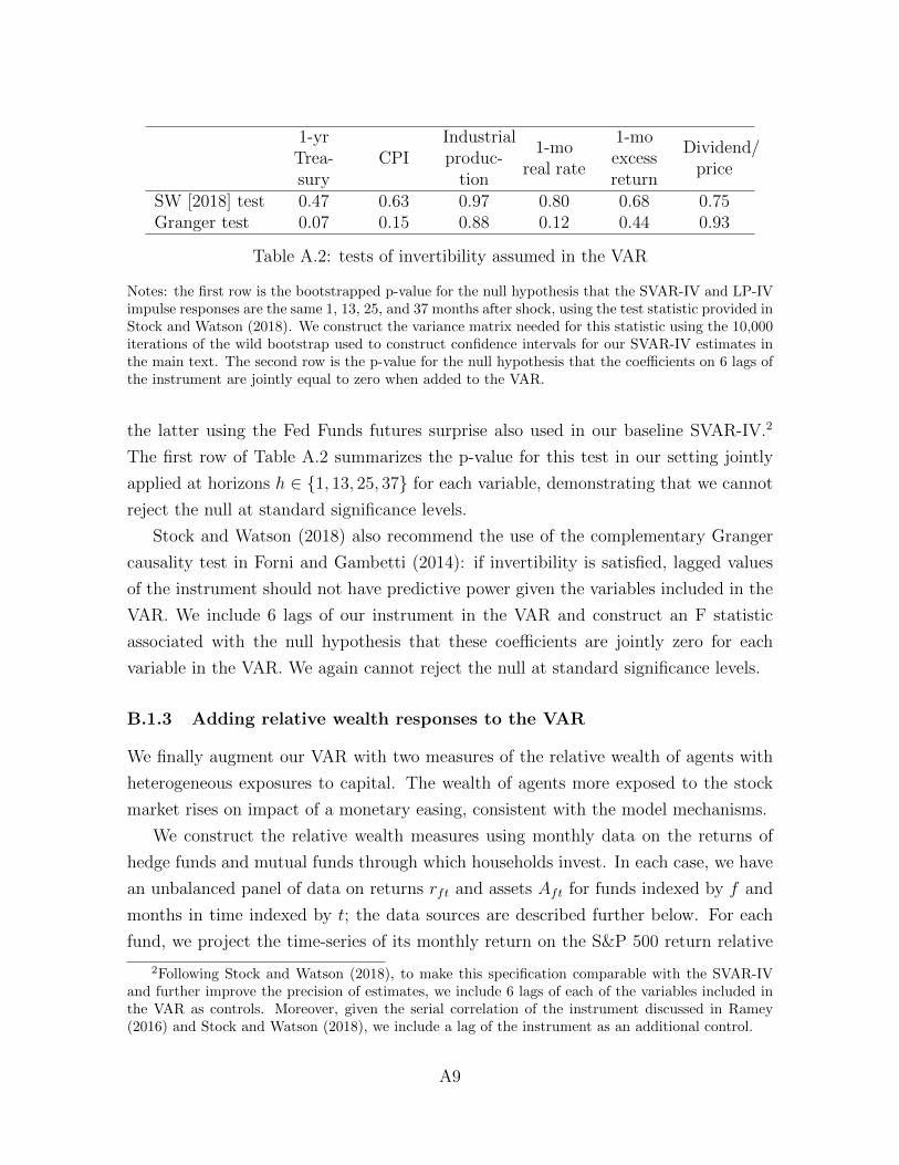
1-yrTrea-sury
CPIIndustrialproduc-
tion
1-moreal rate
1-moexcessreturn
Dividend/price
SW [2018] test 0.47 0.63 0.97 0.80 0.68 0.75Granger test 0.07 0.15 0.88 0.12 0.44 0.93
Table A.2: tests of invertibility assumed in the VAR
Notes: the first row is the bootstrapped p-value for the null hypothesis that the SVAR-IV and LP-IVimpulse responses are the same 1, 13, 25, and 37 months after shock, using the test statistic provided inStock and Watson (2018). We construct the variance matrix needed for this statistic using the 10,000iterations of the wild bootstrap used to construct confidence intervals for our SVAR-IV estimates inthe main text. The second row is the p-value for the null hypothesis that the coefficients on 6 lags ofthe instrument are jointly equal to zero when added to the VAR.
the latter using the Fed Funds futures surprise also used in our baseline SVAR-IV.2
The first row of Table A.2 summarizes the p-value for this test in our setting jointly
applied at horizons h ∈ {1, 13, 25, 37} for each variable, demonstrating that we cannot
reject the null at standard significance levels.
Stock and Watson (2018) also recommend the use of the complementary Granger
causality test in Forni and Gambetti (2014): if invertibility is satisfied, lagged values
of the instrument should not have predictive power given the variables included in the
VAR. We include 6 lags of our instrument in the VAR and construct an F statistic
associated with the null hypothesis that these coefficients are jointly zero for each
variable in the VAR. We again cannot reject the null at standard significance levels.
B.1.3 Adding relative wealth responses to the VAR
We finally augment our VAR with two measures of the relative wealth of agents with
heterogeneous exposures to capital. The wealth of agents more exposed to the stock
market rises on impact of a monetary easing, consistent with the model mechanisms.
We construct the relative wealth measures using monthly data on the returns of
hedge funds and mutual funds through which households invest. In each case, we have
an unbalanced panel of data on returns rft and assets Aft for funds indexed by f and
months in time indexed by t; the data sources are described further below. For each
fund, we project the time-series of its monthly return on the S&P 500 return relative
2Following Stock and Watson (2018), to make this specification comparable with the SVAR-IVand further improve the precision of estimates, we include 6 lags of each of the variables included inthe VAR as controls. Moreover, given the serial correlation of the instrument discussed in Ramey(2016) and Stock and Watson (2018), we include a lag of the instrument as an additional control.
A9
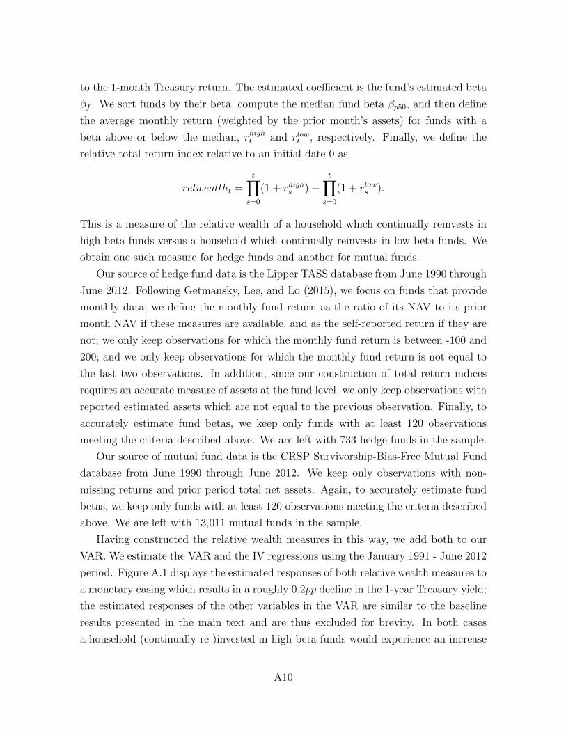
to the 1-month Treasury return. The estimated coefficient is the fund’s estimated beta
βf . We sort funds by their beta, compute the median fund beta βp50, and then define
the average monthly return (weighted by the prior month’s assets) for funds with a
beta above or below the median, rhight and rlowt , respectively. Finally, we define the
relative total return index relative to an initial date 0 as
relwealtht =t∏
s=0
(1 + rhighs )−t∏
s=0
(1 + rlows ).
This is a measure of the relative wealth of a household which continually reinvests in
high beta funds versus a household which continually reinvests in low beta funds. We
obtain one such measure for hedge funds and another for mutual funds.
Our source of hedge fund data is the Lipper TASS database from June 1990 through
June 2012. Following Getmansky, Lee, and Lo (2015), we focus on funds that provide
monthly data; we define the monthly fund return as the ratio of its NAV to its prior
month NAV if these measures are available, and as the self-reported return if they are
not; we only keep observations for which the monthly fund return is between -100 and
200; and we only keep observations for which the monthly fund return is not equal to
the last two observations. In addition, since our construction of total return indices
requires an accurate measure of assets at the fund level, we only keep observations with
reported estimated assets which are not equal to the previous observation. Finally, to
accurately estimate fund betas, we keep only funds with at least 120 observations
meeting the criteria described above. We are left with 733 hedge funds in the sample.
Our source of mutual fund data is the CRSP Survivorship-Bias-Free Mutual Fund
database from June 1990 through June 2012. We keep only observations with non-
missing returns and prior period total net assets. Again, to accurately estimate fund
betas, we keep only funds with at least 120 observations meeting the criteria described
above. We are left with 13,011 mutual funds in the sample.
Having constructed the relative wealth measures in this way, we add both to our
VAR. We estimate the VAR and the IV regressions using the January 1991 - June 2012
period. Figure A.1 displays the estimated responses of both relative wealth measures to
a monetary easing which results in a roughly 0.2pp decline in the 1-year Treasury yield;
the estimated responses of the other variables in the VAR are similar to the baseline
results presented in the main text and are thus excluded for brevity. In both cases
a household (continually re-)invested in high beta funds would experience an increase
A10
0 20 40-2
0
2
pp
Relative wealth,high beta hedge funds
0 20 40-2
0
2
pp
Relative wealth,high beta mutual funds
Figure A.1: effects of a 1 SD monetary shock on relative wealth measures
Notes: see notes accompanying Figure 1 in main text.
in relative wealth on impact of a monetary easing, after which its wealth share would
decline.3 We emphasize that this result is not mechanical: while the hedge funds and
mutual funds are sorted based on their unconditional betas over the sample period,
these measures of relative reported returns do not otherwise use any information on
market returns, and their conditional response to a monetary easing need not have
exhibited the same qualitative pattern as the excess S&P 500 return — but they do.
B.2 Micro moments from the SCF
B.2.1 Construction of household portfolios
We now provide supplemental details on our measurement of household portfolios using
the 2016 SCF described in section 3.3. We proceed in five steps.
First, to the SCF data we add an estimate of defined benefit pension wealth for
each household, since this is not included in the SCF measure of net worth. We use
the estimates of Sabelhaus and Volz (2019).
Second, we proceed by line item to allocate how much household wealth is in directly
held claims on capital, indirect claims on capital through business equity, or nominal
claims. Direct claims on capital are non-financial assets (vehicles, primary residence,
residential real estate excluding the primary residence, non-residential real estate, and
other miscellaneous non-financial assets). Indirect claims on capital through business
equity come in two forms: publicly traded stocks or privately-owned businesses. We
3The larger response of the relative wealth measure using mutual funds is consistent with the factthat we estimate a larger dispersion in betas in the sample of mutual funds than hedge funds.
A11
assume the following line items reported in the SCF summary extract include stocks:4
stock mutual funds, other mutual funds, and directly held stocks, all of which we assume
are fully invested in stocks; combination mutual funds, 50% of which we assume are
invested in stocks; and savings accounts that may be invested in stocks and are included
in transaction accounts (such as 529 or state-sponsored education accounts), other
managed assets, and quasi-liquid retirement assets, for which we use the self-reported
fraction of these accounts invested in stocks. We assume the remaining portion of these
line items not invested in stocks, as well as all other line items not mentioned above,
are purely nominal assets or liabilities.
Third, we assume a functional form for households’ leverage through these equity
claims. We assume that the leverage of publicly traded stocks held by household i is
levipublic = levpublicεi
and the leverage of private businesses owned by household i is
leviprivate = levprivateεi,
where the idiosyncratic component εi is drawn from a Γ(θ−1, θ) distribution having
mean one. levpublic thus reflects the aggregate leverage of the household sector in
publicly traded stocks; levprivate reflects the aggregate leverage of the household sector
in private businesses; and θ controls the dispersion of household leverage in these
claims. The Γ distribution is right-skewed, which accords well with the heterogeneity
in portfolios studied by Calvet, Campbell, and Sodini (2007) and the recent papers on
household returns discussed below.
Fourth, we use the FA to discipline levpublic and levprivate. We set levpublic to the
net leverage of the consolidated nonfinancial corporate sector (FA table S.5.a) and
financial business sector (FA table S.6.a), net of the central bank (FA table S.61.a),
government DB pension funds (FA tables L.119.b and L.120.b), all defined contribution
(DC) pension funds (FA tables L.118.c, L.119.c, and L.120.c), and mutual funds (FA
table L.122).5 We set levprivate to the net leverage of the consolidated nonfinancial
4Our approach here follows the construction of the EQUITY variable in the summary extract.5We exclude the central bank and government DB pension funds because we model these as part
of the government sector (the latter consistent with our interpretation of DB pensions in footnote 24).We exclude DC pension funds and mutual funds because we view these as pure pass-through entitieswhose assets have already been folded into that of households using our approach described so far.
A12
noncorporate sector (FA table S.4.a) and non-profit sector (FA table B.101.n). We
compute net leverage by dividing the aggregate position in capital by net equity issued
to other sectors. Capital is given by total assets net of nominal assets and equity assets.
Net equity issued to other sectors is given by equity liabilities plus net worth net of
equity assets. Using the Q2 2019 release of the FA, the resulting measures of 2016
leverage we obtain are levpublic = 1.6 and levprivate = 1.1.
Using these steps, we decompose the $104,721bn in total U.S. household net worth
(∑
iAi) into $11,228bn in nominal claims (
∑iB
i) and $93,492bn in capital (∑
iQki).6
Fifth and finally, we use recent evidence on the heterogeneity in households’ ex-
pected returns on wealth to discipline θ. Using granular data on the portfolios of the
universe of Swedish households, Bach, Calvet, and Sodini (2018) construct household-
specific measures of expected excess returns. Over the 2000-2007 period, the cross-
sectional standard deviation in expected excess returns on gross assets was 32% of the
expected excess returns of the global market.7 We choose θ = 1.18 so that the implied
cross-sectional standard deviation in leverage on assets in our SCF sample equals 32%
of the aggregate leverage in public equities estimated above (levpublic = 1.6). The fact
that a positive value of θ is needed to match the evidence on return heterogeneity
is consistent with broader results from the literature that households in fact do not
hold identical, diversified equity portfolios.8 Nonetheless, even when θ → 0, in which
case households hold the same, diversified portfolio of equity claims, there is hetero-
geneity in capital portfolio shares (and thus expected returns) because of households’
heterogeneous portfolios across nominal claims, capital, and equity.
B.2.2 Application to the 2007-2009 SCF panel
Using the 2007-2009 SCF panel, we can apply the exact same methodology as described
in the prior subsection to characterize households’ portfolios and sort them into three
groups as of 2007. In this subsection, we follow these households over the next two
6We have validated that this aggregate balance sheet is consistent with market clearing in nominalclaims after accounting for the balance sheets of the government and rest of the world. We refer thereader to the January 2020 working paper version of this paper for further details on this analysis.
7In their Table VI, these authors report a cross-sectional standard deviation in expected excessreturns of 1.9%. In their section I.D., they report a long-run (1983-2016) average of the global marketexcess return of 5.8%. The ratio between these is 32%. We use this evidence from Scandinavia becauseof the absence of comparable data in the United States with exhaustive coverage of households’ wealth.
8It is also consistent with the fact that some households invest in equity through levered investmentintermediaries such as hedge funds and private equity, which cannot be explicitly identified in the SCF.
A13
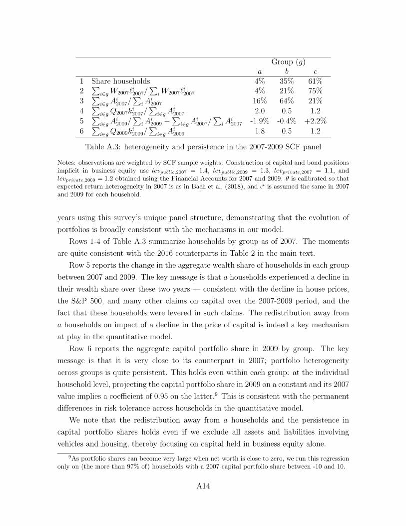
Group (g)a b c
1 Share households 4% 35% 61%2∑
i∈gW2007`i2007/
∑iW2007`
i2007 4% 21% 75%
3∑
i∈g Ai2007/
∑iA
i2007 16% 64% 21%
4∑
i∈gQ2007ki2007/
∑i∈g A
i2007 2.0 0.5 1.2
5∑
i∈g Ai2009/
∑iA
i2009 −
∑i∈g A
i2007/
∑iA
i2007 -1.9% -0.4% +2.2%
6∑
i∈gQ2009ki2009/
∑i∈g A
i2009 1.8 0.5 1.2
Table A.3: heterogeneity and persistence in the 2007-2009 SCF panel
Notes: observations are weighted by SCF sample weights. Construction of capital and bond positionsimplicit in business equity use levpublic,2007 = 1.4, levpublic,2009 = 1.3, levprivate,2007 = 1.1, andlevprivate,2009 = 1.2 obtained using the Financial Accounts for 2007 and 2009. θ is calibrated so thatexpected return heterogeneity in 2007 is as in Bach et al. (2018), and εi is assumed the same in 2007and 2009 for each household.
years using this survey’s unique panel structure, demonstrating that the evolution of
portfolios is broadly consistent with the mechanisms in our model.
Rows 1-4 of Table A.3 summarize households by group as of 2007. The moments
are quite consistent with the 2016 counterparts in Table 2 in the main text.
Row 5 reports the change in the aggregate wealth share of households in each group
between 2007 and 2009. The key message is that a households experienced a decline in
their wealth share over these two years — consistent with the decline in house prices,
the S&P 500, and many other claims on capital over the 2007-2009 period, and the
fact that these households were levered in such claims. The redistribution away from
a households on impact of a decline in the price of capital is indeed a key mechanism
at play in the quantitative model.
Row 6 reports the aggregate capital portfolio share in 2009 by group. The key
message is that it is very close to its counterpart in 2007; portfolio heterogeneity
across groups is quite persistent. This holds even within each group: at the individual
household level, projecting the capital portfolio share in 2009 on a constant and its 2007
value implies a coefficient of 0.95 on the latter.9 This is consistent with the permanent
differences in risk tolerance across households in the quantitative model.
We note that the redistribution away from a households and the persistence in
capital portfolio shares holds even if we exclude all assets and liabilities involving
vehicles and housing, thereby focusing on capital held in business equity alone.
9As portfolio shares can become very large when net worth is close to zero, we run this regressiononly on (the more than 97% of) households with a 2007 capital portfolio share between -10 and 10.
A14
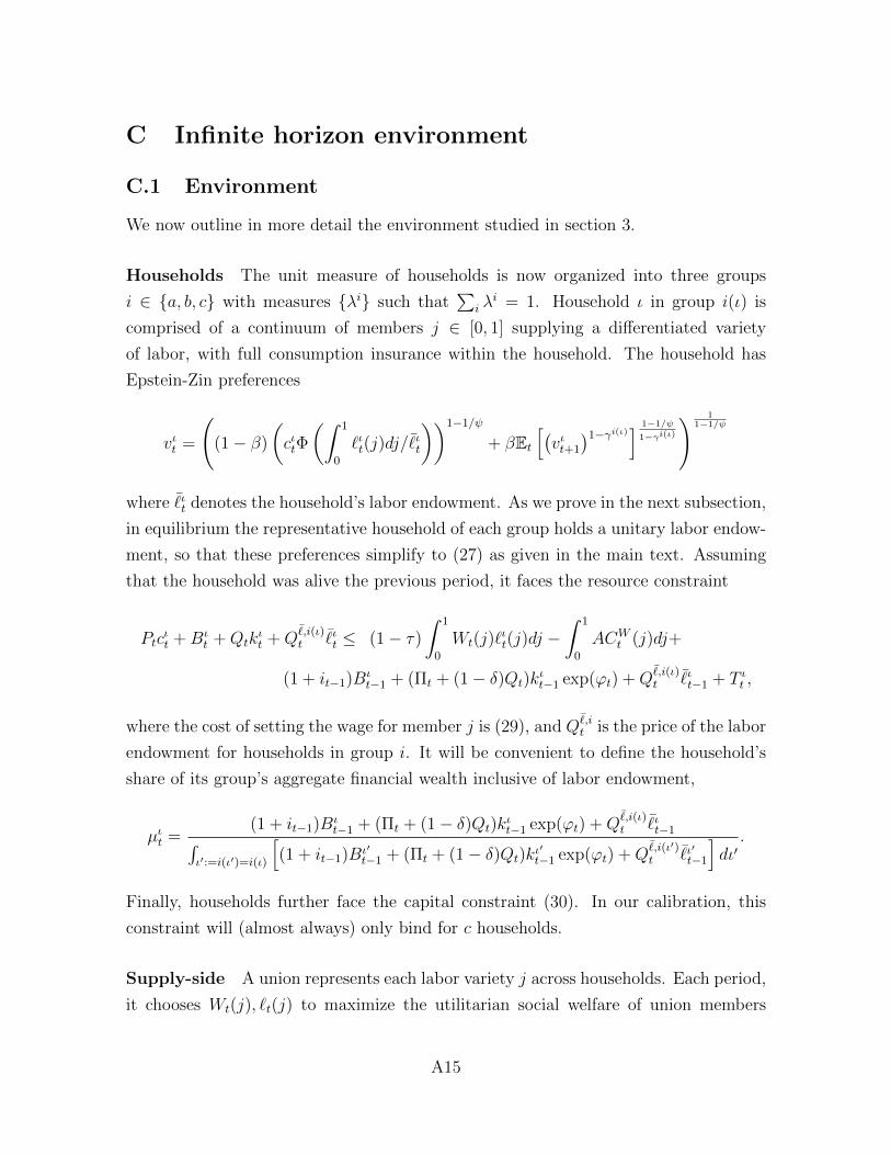
C Infinite horizon environment
C.1 Environment
We now outline in more detail the environment studied in section 3.
Households The unit measure of households is now organized into three groups
i ∈ {a, b, c} with measures {λi} such that∑
i λi = 1. Household ι in group i(ι) is
comprised of a continuum of members j ∈ [0, 1] supplying a differentiated variety
of labor, with full consumption insurance within the household. The household has
Epstein-Zin preferences
vιt =
((1− β)
(cιtΦ
(∫ 1
0
`ιt(j)dj/¯ιt
))1−1/ψ
+ βEt[(vιt+1
)1−γi(ι)] 1−1/ψ
1−γi(ι)
) 11−1/ψ
where ¯ιt denotes the household’s labor endowment. As we prove in the next subsection,
in equilibrium the representative household of each group holds a unitary labor endow-
ment, so that these preferences simplify to (27) as given in the main text. Assuming
that the household was alive the previous period, it faces the resource constraint
Ptcιt +Bι
t +Qtkιt +Q
¯,i(ι)t
¯ιt ≤ (1− τ)
∫ 1
0
Wt(j)`ιt(j)dj −
∫ 1
0
ACWt (j)dj+
(1 + it−1)Bιt−1 + (Πt + (1− δ)Qt)k
ιt−1 exp(ϕt) +Q
¯,i(ι)t
¯ιt−1 + T ιt ,
where the cost of setting the wage for member j is (29), and Q¯,it is the price of the labor
endowment for households in group i. It will be convenient to define the household’s
share of its group’s aggregate financial wealth inclusive of labor endowment,
µιt =(1 + it−1)Bι
t−1 + (Πt + (1− δ)Qt)kιt−1 exp(ϕt) +Q
¯,i(ι)t
¯ιt−1∫
ι′:=i(ι′)=i(ι)
[(1 + it−1)Bι′
t−1 + (Πt + (1− δ)Qt)kι′t−1 exp(ϕt) +Q
¯,i(ι′)t
¯ι′t−1
]dι′.
Finally, households further face the capital constraint (30). In our calibration, this
constraint will (almost always) only bind for c households.
Supply-side A union represents each labor variety j across households. Each period,
it chooses Wt(j), `t(j) to maximize the utilitarian social welfare of union members
A15
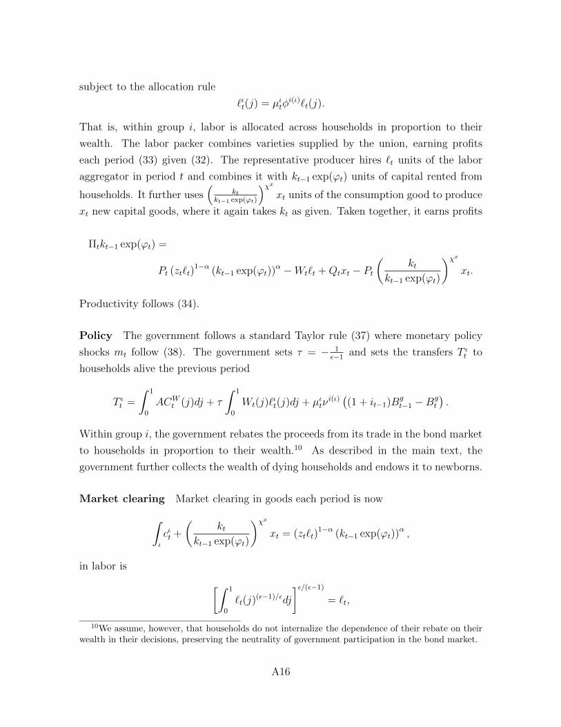
subject to the allocation rule
`ιt(j) = µιtφi(ι)`t(j).
That is, within group i, labor is allocated across households in proportion to their
wealth. The labor packer combines varieties supplied by the union, earning profits
each period (33) given (32). The representative producer hires `t units of the labor
aggregator in period t and combines it with kt−1 exp(ϕt) units of capital rented from
households. It further uses(
ktkt−1 exp(ϕt)
)χxxt units of the consumption good to produce
xt new capital goods, where it again takes kt as given. Taken together, it earns profits
Πtkt−1 exp(ϕt) =
Pt (zt`t)1−α (kt−1 exp(ϕt))
α −Wt`t +Qtxt − Pt(
ktkt−1 exp(ϕt)
)χxxt.
Productivity follows (34).
Policy The government follows a standard Taylor rule (37) where monetary policy
shocks mt follow (38). The government sets τ = − 1ε−1
and sets the transfers T ιt to
households alive the previous period
T ιt =
∫ 1
0
ACWt (j)dj + τ
∫ 1
0
Wt(j)`ιt(j)dj + µιtν
i(ι)((1 + it−1)Bg
t−1 −Bgt
).
Within group i, the government rebates the proceeds from its trade in the bond market
to households in proportion to their wealth.10 As described in the main text, the
government further collects the wealth of dying households and endows it to newborns.
Market clearing Market clearing in goods each period is now∫ι
cιt +
(kt
kt−1 exp(ϕt)
)χxxt = (zt`t)
1−α (kt−1 exp(ϕt))α ,
in labor is [∫ 1
0
`t(j)(ε−1)/εdj
]ε/(ε−1)
= `t,
10We assume, however, that households do not internalize the dependence of their rebate on theirwealth in their decisions, preserving the neutrality of government participation in the bond market.
A16
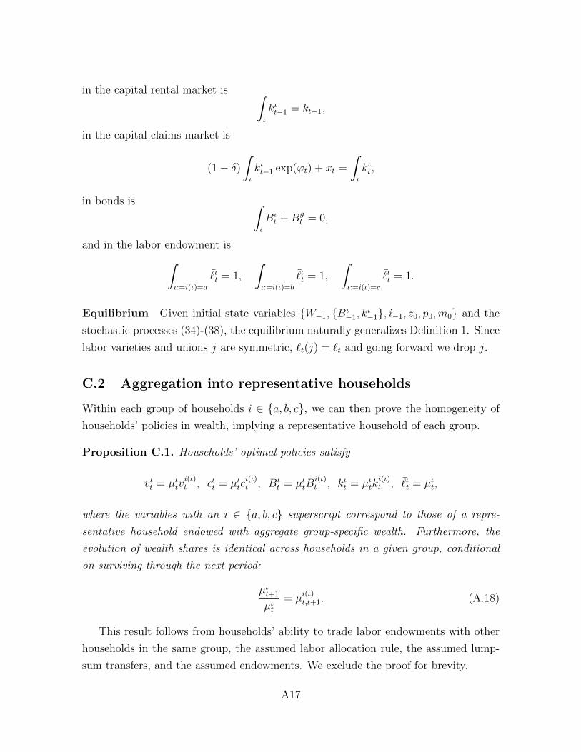
in the capital rental market is ∫ι
kιt−1 = kt−1,
in the capital claims market is
(1− δ)∫ι
kιt−1 exp(ϕt) + xt =
∫ι
kιt,
in bonds is ∫ι
Bιt +Bg
t = 0,
and in the labor endowment is∫ι:=i(ι)=a
¯ιt = 1,
∫ι:=i(ι)=b
¯ιt = 1,
∫ι:=i(ι)=c
¯ιt = 1.
Equilibrium Given initial state variables {W−1, {Bι−1, k
ι−1}, i−1, z0, p0,m0} and the
stochastic processes (34)-(38), the equilibrium naturally generalizes Definition 1. Since
labor varieties and unions j are symmetric, `t(j) = `t and going forward we drop j.
C.2 Aggregation into representative households
Within each group of households i ∈ {a, b, c}, we can then prove the homogeneity of
households’ policies in wealth, implying a representative household of each group.
Proposition C.1. Households’ optimal policies satisfy
vιt = µιtvi(ι)t , cιt = µιtc
i(ι)t , Bι
t = µιtBi(ι)t , kιt = µιtk
i(ι)t , ¯ι
t = µιt,
where the variables with an i ∈ {a, b, c} superscript correspond to those of a repre-
sentative household endowed with aggregate group-specific wealth. Furthermore, the
evolution of wealth shares is identical across households in a given group, conditional
on surviving through the next period:
µιt+1
µιt= µ
i(ι)t,t+1. (A.18)
This result follows from households’ ability to trade labor endowments with other
households in the same group, the assumed labor allocation rule, the assumed lump-
sum transfers, and the assumed endowments. We exclude the proof for brevity.
A17
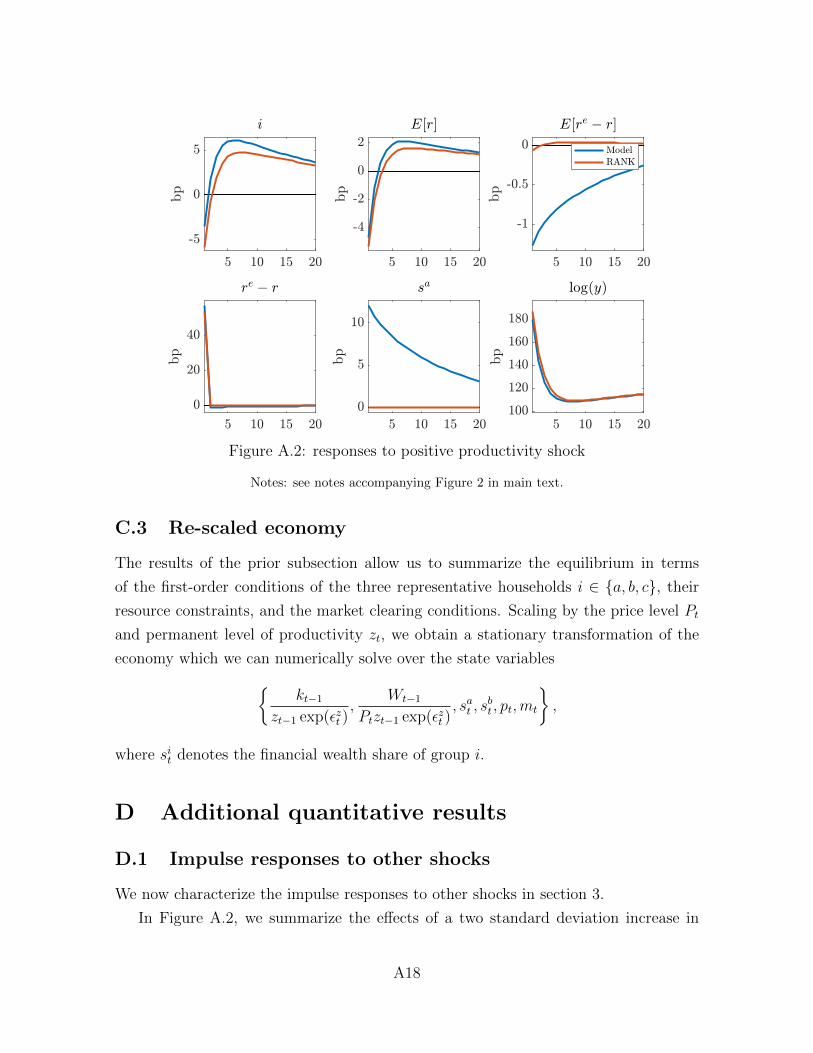
Figure A.2: responses to positive productivity shock
Notes: see notes accompanying Figure 2 in main text.
C.3 Re-scaled economy
The results of the prior subsection allow us to summarize the equilibrium in terms
of the first-order conditions of the three representative households i ∈ {a, b, c}, their
resource constraints, and the market clearing conditions. Scaling by the price level Pt
and permanent level of productivity zt, we obtain a stationary transformation of the
economy which we can numerically solve over the state variables{kt−1
zt−1 exp(εzt ),
Wt−1
Ptzt−1 exp(εzt ), sat , s
bt , pt,mt
},
where sit denotes the financial wealth share of group i.
D Additional quantitative results
D.1 Impulse responses to other shocks
We now characterize the impulse responses to other shocks in section 3.
In Figure A.2, we summarize the effects of a two standard deviation increase in
A18
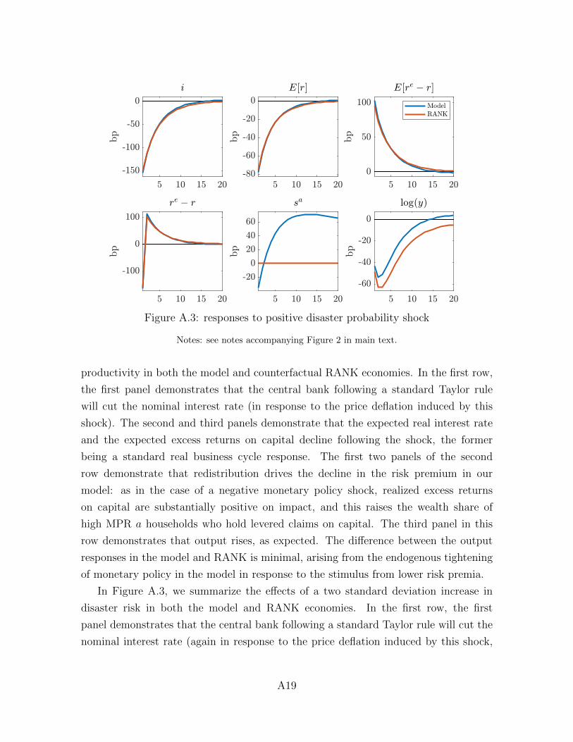
Figure A.3: responses to positive disaster probability shock
Notes: see notes accompanying Figure 2 in main text.
productivity in both the model and counterfactual RANK economies. In the first row,
the first panel demonstrates that the central bank following a standard Taylor rule
will cut the nominal interest rate (in response to the price deflation induced by this
shock). The second and third panels demonstrate that the expected real interest rate
and the expected excess returns on capital decline following the shock, the former
being a standard real business cycle response. The first two panels of the second
row demonstrate that redistribution drives the decline in the risk premium in our
model: as in the case of a negative monetary policy shock, realized excess returns
on capital are substantially positive on impact, and this raises the wealth share of
high MPR a households who hold levered claims on capital. The third panel in this
row demonstrates that output rises, as expected. The difference between the output
responses in the model and RANK is minimal, arising from the endogenous tightening
of monetary policy in the model in response to the stimulus from lower risk premia.
In Figure A.3, we summarize the effects of a two standard deviation increase in
disaster risk in both the model and RANK economies. In the first row, the first
panel demonstrates that the central bank following a standard Taylor rule will cut the
nominal interest rate (again in response to the price deflation induced by this shock,
A19
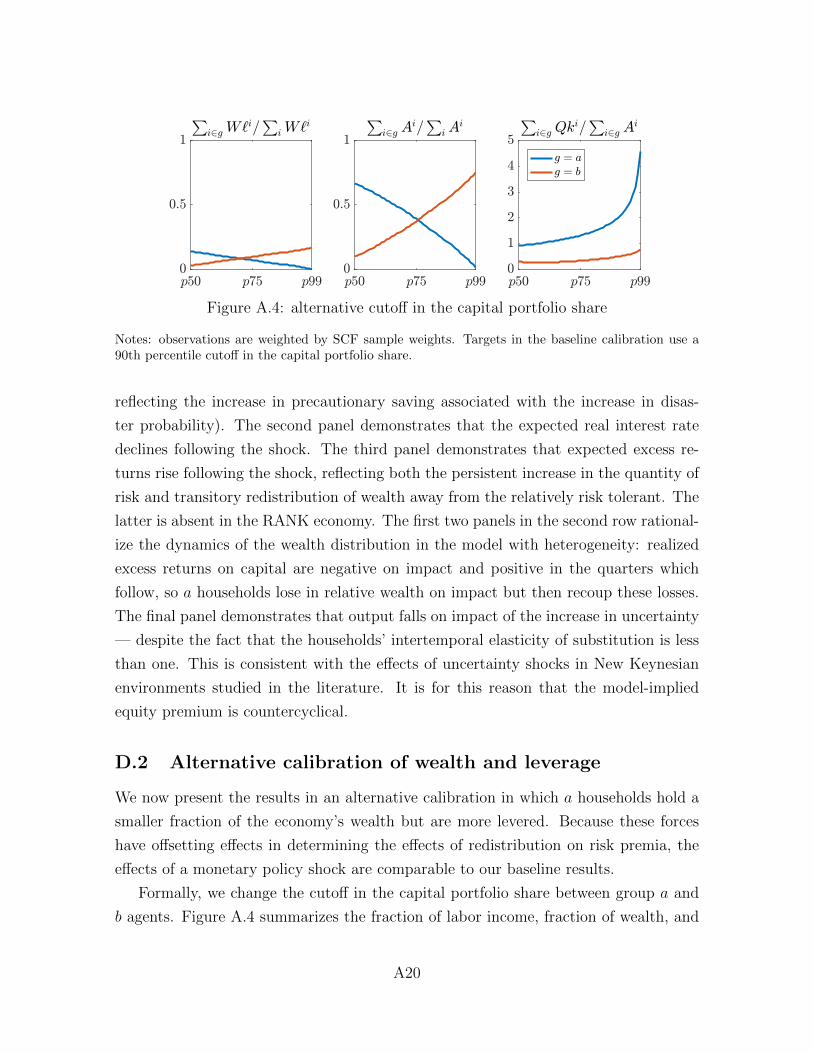
p50 p75 p99Qki=Ai
0
0.5
1
Pi2g W`i=
Pi W`i
p50 p75 p99Qki=Ai
0
0.5
1
Pi2g Ai=
Pi A
i
p50 p75 p99Qki=Ai
0
1
2
3
4
5
Pi2g Qki=
Pi2g Ai
g = ag = b
Figure A.4: alternative cutoff in the capital portfolio share
Notes: observations are weighted by SCF sample weights. Targets in the baseline calibration use a90th percentile cutoff in the capital portfolio share.
reflecting the increase in precautionary saving associated with the increase in disas-
ter probability). The second panel demonstrates that the expected real interest rate
declines following the shock. The third panel demonstrates that expected excess re-
turns rise following the shock, reflecting both the persistent increase in the quantity of
risk and transitory redistribution of wealth away from the relatively risk tolerant. The
latter is absent in the RANK economy. The first two panels in the second row rational-
ize the dynamics of the wealth distribution in the model with heterogeneity: realized
excess returns on capital are negative on impact and positive in the quarters which
follow, so a households lose in relative wealth on impact but then recoup these losses.
The final panel demonstrates that output falls on impact of the increase in uncertainty
— despite the fact that the households’ intertemporal elasticity of substitution is less
than one. This is consistent with the effects of uncertainty shocks in New Keynesian
environments studied in the literature. It is for this reason that the model-implied
equity premium is countercyclical.
D.2 Alternative calibration of wealth and leverage
We now present the results in an alternative calibration in which a households hold a
smaller fraction of the economy’s wealth but are more levered. Because these forces
have offsetting effects in determining the effects of redistribution on risk premia, the
effects of a monetary policy shock are comparable to our baseline results.
Formally, we change the cutoff in the capital portfolio share between group a and
b agents. Figure A.4 summarizes the fraction of labor income, fraction of wealth, and
A20
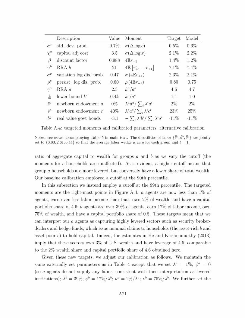
Description Value Moment Target Model
σz std. dev. prod. 0.7% σ(∆ log c) 0.5% 0.6%
χx capital adj cost 3.5 σ(∆ log x) 2.1% 2.2%
β discount factor 0.988 4Er+1 1.4% 1.2%
γb RRA b 21 4E[re+1 − r+1
]7.1% 7.4%
σp variation log dis. prob. 0.47 σ (4Er+1) 2.3% 2.1%
ρp persist. log dis. prob. 0.80 ρ (4Er+1) 0.80 0.75
γa RRA a 2.5 ka/aa 4.6 4.7
k lower bound ki 0.4k kc/ac 1.1 1.0
sa newborn endowment a 0% λaaa/∑
i λiai 2% 2%
sc newborn endowment c 40% λcac/∑
i λici 23% 25%
bg real value govt bonds -3.1 −∑
i λibi/
∑i λ
iai -11% -11%
Table A.4: targeted moments and calibrated parameters, alternative calibration
Notes: see notes accompanying Table 5 in main text. The disutilities of labor {θa, θb, θc} are jointlyset to {0.00, 2.61, 0.44} so that the average labor wedge is zero for each group and ` = 1.
ratio of aggregate capital to wealth for groups a and b as we vary the cutoff (the
moments for c households are unaffected). As is evident, a higher cutoff means that
group a households are more levered, but conversely have a lower share of total wealth.
Our baseline calibration employed a cutoff at the 90th percentile.
In this subsection we instead employ a cutoff at the 99th percentile. The targeted
moments are the right-most points in Figure A.4: a agents are now less than 1% of
agents, earn even less labor income than that, own 2% of wealth, and have a capital
portfolio share of 4.6; b agents are over 39% of agents, earn 17% of labor income, own
75% of wealth, and have a capital portfolio share of 0.8. These targets mean that we
can interpret our a agents as capturing highly levered sectors such as security broker-
dealers and hedge funds, which issue nominal claims to households (the asset-rich b and
asset-poor c) to hold capital. Indeed, the estimates in He and Krishnamurthy (2013)
imply that these sectors own 3% of U.S. wealth and have leverage of 4.5, comparable
to the 2% wealth share and capital portfolio share of 4.6 obtained here.
Given these new targets, we adjust our calibration as follows. We maintain the
same externally set parameters as in Table 4 except that we set λa = 1%; φa = 0
(so a agents do not supply any labor, consistent with their interpretation as levered
institutions); λb = 39%; φb = 17%/λb; νa = 2%/λa; νb = 75%/λb. We further set the
A21
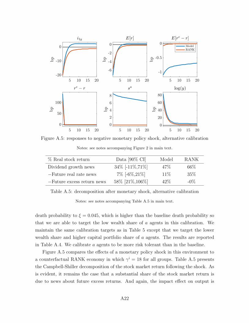
Figure A.5: responses to negative monetary policy shock, alternative calibration
Notes: see notes accompanying Figure 2 in main text.
% Real stock return Data [90% CI] Model RANK
Dividend growth news 34% [-11%,71%] 47% 66%
−Future real rate news 7% [-6%,21%] 11% 35%
−Future excess return news 58% [21%,106%] 42% -0%
Table A.5: decomposition after monetary shock, alternative calibration
Notes: see notes accompanying Table A.5 in main text.
death probability to ξ = 0.045, which is higher than the baseline death probability so
that we are able to target the low wealth share of a agents in this calibration. We
maintain the same calibration targets as in Table 5 except that we target the lower
wealth share and higher capital portfolio share of a agents. The results are reported
in Table A.4. We calibrate a agents to be more risk tolerant than in the baseline.
Figure A.5 compares the effects of a monetary policy shock in this environment to
a counterfactual RANK economy in which γi = 18 for all groups. Table A.5 presents
the Campbell-Shiller decomposition of the stock market return following the shock. As
is evident, it remains the case that a substantial share of the stock market return is
due to news about future excess returns. And again, the impact effect on output is
A22

Description Value Moment Target Model
σz std. dev. prod. 0.6% σ(∆ log c) 0.5% 0.6%
χx capital adj cost 3.5 σ(∆ log x) 2.1% 2.2%
β discount factor 0.993 4Er+1 1.4% 1.5%
γa = γb = γc RRA 12 4E[re+1 − r+1
]7.1% 6.6%
σp variation log dis. prob. 0.83 σ (4Er+1) 2.3% 2.1%
ρp persist. log dis. prob. 0.80 ρ (4Er+1) 0.80 0.75
ηb idio. risk b 0.005 ka/aa 2.0 2.0
k lower bound ki 0.4k kc/ac 1.1 1.1
sa newborn endowment a 0% λaaa/∑
i λiai 18% 21%
sc newborn endowment c 40% λcac/∑
i λici 23% 24%
bg real value govt bonds -3.1 −∑
i λibi/
∑i λ
iai -11% -11%
Table A.6: targeted moments and calibrated parameters, idiosyncratic risk
Notes: see notes accompanying Table 5 in main text. The disutilities of labor {θa, θb, θc} are jointlyset to {0.90, 3.83, 0.45} so that the average labor wedge is zero for each group and ` = 1.
roughly 1.3 times larger than in the RANK economy.
D.3 Alternative microfoundation of portfolio heterogeneity
We now present the results in an alternative environment which microfounds differences
in portfolios and MPRs without appealing to differences in risk aversion. Instead, we
assume households experience idiosyncratic returns on capital, and the volatility of
these returns differs across groups, consistent with one of the alternative forms of
heterogeneity considered in section 2.5. We demonstrate that our quantitative results
are again robust to this setting.
Formally, we assume that households’ choice of capital kit in period t is subject to
an idiosyncratic quality shock at t+1, turning into εit+1kit units of capital which can be
rented in the spot market to firms. The quality shock is an iid shock from a lognormal
distribution, the variance of which is the group-specific parameter ηi:
log εit+1 ∼ N
(−1
2ηi, ηi
).
In equilibrium, this only affects households’ portfolio choice; since the quality shock
A23

Figure A.6: responses to negative monetary policy shock, idiosyncratic risk
Notes: see notes accompanying Figure 2 in main text.
% Real stock return Data [90% CI] Model RANK
Dividend growth news 34% [-11%,71%] 46% 66%
−Future real rate news 7% [-6%,21%] 20% 35%
−Future excess return news 58% [21%,106%] 34% -1%
Table A.7: decomposition after monetary shock, idiosyncratic risk
Notes: see notes accompanying Table A.5 in main text.
has a mean value of one, the representative household still rents kit units of capital and
none of the supply-side conditions or aggregate resource constraints are affected.
To rationalize their high leverage, a households are now calibrated to be those with
the smallest volatility of idiosyncratic returns; equivalently, they have the highest risk-
adjusted returns. Formally, we maintain the same externally set parameters as in Table
4 and set ηa = 0. We then re-calibrate the parameters in Table A.6 assuming that
households share the same level of risk aversion γ calibrated to match the level of the
equity premium, and calibrating ηb and k to match households’ capital portfolio shares.
Taken together, this environment builds on a large literature on entrepreneurship in
macroeconomic models emphasizing idiosyncratic risk and entrepreneurs as those with
A24

relatively good investment ideas.
Figure A.6 compares the effects of a monetary policy shock in this environment
to a counterfactual RANK economy in which ηi is identical across groups. Table A.7
presents the Campbell-Shiller decomposition of the stock market return following the
shock. It remains the case that a substantial share of the stock market return is due to
news about future excess returns. And again, the impact effect on output is roughly
1.4 times larger than in the RANK economy.
References
Bach, L., L. E. Calvet, and P. Sodini (2018): “Rich pickings? Risk, return, andskill in household wealth,” Working paper.
Bernanke, B. S. and K. N. Kuttner (2005): “What explains the stock market’sreaction to Federal Reserve policy?” Journal of Finance, 60, 1221–1257.
Calvet, L. E., J. Y. Campbell, and P. Sodini (2007): “Down or out: assessingthe welfare costs of household investment mistakes,” Journal of Political Economy,115, 707–747.
Forni, M. and L. Gambetti (2014): “Sufficient information in structural VARs,”Journal of Monetary Economics, 66, 124–136.
Gertler, M. and P. Karadi (2015): “Monetary policy surprises, credit costs, andeconomic activity,” American Economic Journal: Macroeconomics, 7, 44–76.
Getmansky, M., P. A. Lee, and A. W. Lo (2015): “Hedge funds: a dynamicindustry in transition,” Annual Review of Financial Economics, 7, 483–577.
Gilchrist, S. and E. Zakrajsek (2012): “Credit spreads and business cycle fluc-tuations,” American Economic Review, 102, 1692–1720.
He, Z. and A. Krishnamurthy (2013): “Intermediary Asset Pricing,” AmericanEconomic Review, 2, 732–770.
Ramey, V. A. (2016): Macroeconomic shocks and their propagation, Elsevier, vol. 2Aof Handbook of Macroeconomics, 71–162.
Sabelhaus, J. and A. H. Volz (2019): “Are disappearing employer pensions con-tributing to rising wealth inequality?” Working paper.
Stock, J. H. and M. W. Watson (2018): “Identification and estimation of dy-namic causal effects in macroeconomics using external instruments,” The EconomicJournal, 128, 917–948.
A25