working paper no. 188 - icrier.org · himanshu (2004a, b) and surjit bhalla (2003) in this regard....
TRANSCRIPT

INDIAN COUNCIL FOR RESEARCH ON INTERNATIONAL ECONOMIC RELATIONS
Working Paper No. 188
The Debate on the Poverty Estimates of 1999–2000
K.L. Datta
October 2006

CONTENTS
Foreword............................................................................................................................... I Abstract................................................................................................................................II The Results ..........................................................................................................................II Poverty Ratio in 1999–2000.............................................................................................. III Number of Poor in 1999–2000 ......................................................................................... III Reduction in Poverty Ratio .............................................................................................. III Reduction in Number of Poor.......................................................................................... III 1 Introduction..............................................................................................................1 1.1 Comparability of NSS 55th Round Consumption ................................................3 1.2 Recent Experiments on the Choice of Recall Period ............................................5 1.3 The Issues and Alternatives ....................................................................................6 2 Poverty Estimates by Angus Deaton ......................................................................7 2.1 Deaton’s Method ......................................................................................................8 2.1.1 The Comparability Problem ...................................................................................9 2.1.2 Alternative Poverty Line .......................................................................................11 2.2 Adjustment of NSS 55th Round Consumer Expenditure Data .........................13 2.3 Deaton’s Poverty Estimates: 1987–8 to 1999–2000.............................................16 2.4 Impact of Recall Period .........................................................................................17 2.5 Impact of Poverty Line and Recall Period ..........................................................18 2.6 Sen–Himanshu on Deaton’s Method....................................................................20 2.7 Deaton on Sen–Himanshu’s Contention ..............................................................23 3 Poverty Estimates by Sundaram–Tendulkar ......................................................24 3.1 The Comparable Estimates of Poverty ................................................................25 3.1.1 Comparability of NSS 50th and 55th Rounds Consumer Expenditure ............25 3.1.2 Impact of Longer Recall Period on Consumption ..............................................30 3.2 Poverty Trends in 1980s and 1990s ......................................................................31 3.3 Deaton’s Observations...........................................................................................33 3.4 Sen–Himanshu on Sundaram–Tendulkar ...........................................................34 4 Poverty Estimates by Sen–Himanshu ..................................................................35 4.1 The Scheme of Poverty Calculation .....................................................................36 4.1.1 Comparability of NSS Consumption....................................................................36 4.1.2 Freeing Food Consumption from Contamination: NSS 55th Round................38 4.1.3 Other Estimates......................................................................................................40 4.2 Sen–Himanshu Poverty Estimates: 1987–8 to 1999–2000..................................40 4.2.1 Poverty Reduction: 1987–8 to 1993–4..................................................................41

4.2.2 Poverty Reduction: 1993–4 to 1999–2000............................................................41 4.3 Comparing the Decline in Poverty .......................................................................42 4.4 URP and MRP Consumption: A Comparison ....................................................44 4.5 Poverty Ratio and Number of Poor......................................................................46 5 Poverty Estimates by Bhalla .................................................................................48 5.1 Ten Findings of Bhalla...........................................................................................48 5.2 Poverty, Inequality and Growth: The Relationships..........................................52 5.3 The View of 1983–2000..........................................................................................54 5.4 Poverty Estimation: The Approach .....................................................................56 5.4.1 Comparability Issues in NSS 55th Round Consumer Expenditure Data .........56 5.4.2 The Poverty Ratios: 1983 to 1999–2000...............................................................59 5.4.3 Poverty Estimate in 1999–2000.............................................................................60 5.5 Exchanges with Deaton..........................................................................................63 5.5.1 Bhalla on Deaton....................................................................................................63 5.5.2 Deaton on Bhalla ....................................................................................................65 5.6 The Relevance of Bhalla’s Estimates....................................................................66 6 National Level Poverty Estimates: A Round Up.................................................66 6.1 The Planning Commission Estimates and its Alternatives ................................68 6.2 The Comparison.....................................................................................................70 6.3 Impact of Recall Period of Five Non-Food items on Poverty.............................73 6.4 Impact of Contamination of Food Data on Poverty ...........................................74 6.5 Impact of Recall Period of Non-Food Items and Contamination of Food
Data on Poverty......................................................................................................74 7 Interpreting Sen–Himanshu Poverty Estimates .................................................75 7.1 Two Comments.......................................................................................................75 7.2 Two Caveats ...........................................................................................................78 7.3 A Simulation Exercise............................................................................................80 7.4 Wrapping Up..........................................................................................................81 References.........................................................................................................................102

LIST OF TABLES
Table 1: Deaton’s Estimates of Poverty Ratio.....................................................................17 Table 2: Poverty Estimates by Sundaram–Tendulkar .......................................................31 Table 3: Poverty Estimates by Sen - Himanshu..................................................................40 Table 4: Decline in Poverty Ratios: A Comparison............................................................43 Table 5: Per Capita Income and Consumption Growth Rates..........................................49 Table 6: Growth Rate of Wages in Rural Areas .................................................................51 Table 7: Poverty Ratio: Bhalla and Planning Commission ...............................................52 Table 8: Poverty Ratio and Number of Poor.......................................................................67 Table 9: Poverty Ratio in 1994-95 and 2000-01 ..................................................................76 Table 10: GDP Growth around 1987-8................................................................................79
LIST OF ANNEXURE
Annexure A: NSS Experiment with Recall Period .............................................................84 Annexure B: Price Adjustment of the Poverty Lines by Deaton–Tarozzi........................91 Annexure C: Poverty Reduction in the 1990s: Sundaram’s Estimates ............................93 Annexure D: NAS-NSS Consumption Differential and Poverty Estimation ..................96

I
Foreword
This Working Paper examines the issue of comparability of the latest poverty
estimates prepared by the Planning Commission for the year 1999–2000, with earlier
estimates of the 1980s and 1990s focusing on the methodology and database of
estimation. It also reviews the literature to discuss the relevance of alternative
approaches in this regard. On this basis, the paper assesses the magnitude of poverty
reduction during the two decades. It is hoped that this effort will contribute to a
clearer understanding of the nature and extent of poverty in the country.
(Rajiv Kumar) Director & Chief Executive
October 9, 2006

II
Abstract
This paper compares the latest estimates of poverty (1999–2000) made by the
Planning Commission with earlier estimates of the 1980s and 1990s, focusing on the
methodology and database used for estimation. It extensively reviews the attempts by
Angus Deaton (2003a, b, and c), Sundaram and Tendulkar (2001; 2003a, d), Sen-
Himanshu (2004a, b) and Surjit Bhalla (2003) in this regard. The paper traces the
comparable poverty estimates for the 1980s and 1990s in their levels and change and
uses the extent of poverty reduction implicit in these estimates to assess the
magnitude of poverty reduction in the two decades. These are placed in the wider
debate on the impact of the economic reform programmes on the incidence of poverty
in the Indian context.
The Results
The Planning Commission using NSS consumer expenditure data of 55th Round
estimated the poverty ratio in 1999–2000 as 26.1 per cent. The poverty estimates of
1999–2000 are not comparable with the earlier estimates, namely, for the years 1973–
4, 1977–8, 1983, 1987–8 and 1993–4 because the method of collection of consumer
expenditure data in the 55th Round was different from the earlier Rounds.
There are two reasons for this. First, food consumption data was collected from 7-day
and 30-day recall periods from the same household at the same time. This, according
to many, introduced simultaneity in the food consumption data. Second, for five
infrequently purchased non-food items, the consumption data was gathered from 365-
day recall period. In the earlier years, the poverty estimates were based on the
consumption derived from 30-day recall period for these items.
The poverty ratios and estimates derived by Deaton, Sundaram–Tendulkar and Sen–
Himanshu are relevant in this context because these are important attempts to make
NSS 55th Round consumer expenditure data comparable with the earlier rounds.

III
Poverty Ratio in 1999–2000 Rural Urban Total 1. Deaton 30.0 24.7 28.5 2. Sundaram–Tendulkar 28.9 23.1 27.3 3. Sen–Himanshu 28.8 25.1 27.8 4. Planning Commission 27.1 23.6 26.1
Number of Poor in 1999–2000
(million) Rural Urban Total 1. Deaton 213.9 70.1 284.0 2. Sundaram–Tendulkar 210.5 63.8 274.3 3. Sen–Himanshu 205.3 71.3 276.6 4. Planning Commission 193.2 67.0 260.2
Reduction in Poverty Ratio
(percentage points) 1983 to
1993-4 1987–8 to 1993–4
1993–4 to 1999–2000
1. Deaton – 3.4 7.5 2. Sundaram–Tendulkar 9.1 – 4.9 3. Sen–Himanshu – 4.3 2.8 4. Planning Commission 8.4 2.9 9.9
Note: – indicates that the estimate is not available.
Reduction in Number of Poor
(million) 1983
to 1993–4
1987–8 to 1993–4
1993–4 to 1999–2000
1. Deaton – -9.5 36.2 2. Sundaram–Tendulkar -0.2 – 13.1 3. Sen–Himanshu – 2.9 -4.2 4. Planning Commission 2.6 -13.2 60.1
Note: 1. Negative sign indicates increase in the number of poor. 2. – indicates that the estimate is not available.

1
The Debate on the Poverty Estimates of 1999–2000
1 Introduction
Measurement of the extent of poverty, trends over time and the role of economic
policy and development strategy in reducing poverty have been at the centre of the
policy debate in India.1 The debate on poverty in this context has traditionally been
focused on the methodology of estimation. But, the debate on the poverty estimate of
1999–2000, unlike the earlier ones, has National Sample Survey (NSS) data on
consumer expenditure at its centre.
The Planning Commission is the nodal agency of the Government of India for
estimation of poverty in the country. It estimates the number and percentage of people
living below the poverty line at the national and state level in rural and urban areas
from large sample survey of consumer expenditure conducted by the National Sample
Survey Organisation (NSSO) of the Ministry of Statistics and Programme
Implementation. The methodology of estimation is based on the recommendations of
the Expert Group on Estimation of Proportion and Number of Poor.2 Under this
method, the national level poverty ratios are estimated from the state-specific poverty
ratios (separately in rural and urban areas). The state-specific poverty ratios are
estimated from the state-specific poverty lines and the large sample survey of NSS
consumer expenditure data. Following this method, the Planning Commission in the
past estimated poverty ratio (the ratio of the number of poor to the total population,
expressed as percentage) at the national and state level for the years 1973–4, 1977–8,
1983, 1987–8 and 1993–4.3 The latest estimate of poverty released by the Planning
1 Foreword by Montek Singh Ahluwalia, in The Great Indian Poverty Debate, Deaton-Kozel (eds).
Macmillan India (2005), page iv. 2 Report of the Expert Group on Estimation of Proportion and Number of Poor, Perspective Planning
Division, Planning Commission, Government of India, 1993. Also known as Lakdawala Committee named after its Chairman.
3 Poverty estimates for the years 1973–4, 1977–8, 1983, 1987–8 and 1993–4 made by the Planning Commission on the basis of the Expert Group methodology were released through a Press Note of the Government of India. For details see: Press Information Bureau (1997), ‘Estimates of Poverty’, 11 March, 1997, Government of India.
2
Commission relates to the year 1999–2000 and this is derived from NSS consumer
expenditure data of the 55th Round using the Expert Group methodology.4
The Government of India, in July 1991 launched a major economic reform
programme, which was characterized by ‘re-orientation of economic policy, away
from the earlier control-oriented economic system with a dominant role for the public
sector to a more liberal system with a much greater role for markets and the private
sector, and a gradual opening of the economy to the world trade and foreign
investment.’5 The poverty estimates of 1999–2000 were eagerly awaited for the
assessment of the impact of these policy shifts (which were equated with the
economic reforms and liberalization measures of the government) on the levels of
living of the population, in general, and on the poor, in particular. But, the National
Sample Survey data of consumer expenditure, which was used by the Planning
Commission to measure the incidence of poverty in 1999–2000, was subject to debate
by planners and policy makers for lack of comparability with those of the earlier
years. The loss of comparability arose from the manner and method of collection of
consumer expenditure data in the 55th Round of NSS, which made this data non-
comparable with those of the earlier rounds of large sample surveys; the non-
comparability arose from the experiment with the recall period in NSS 55th Round.
The non-comparability of the estimates of poverty in 1999–2000 with the earlier ones
posed a hurdle in the assessment of the change in the poverty situation, particularly in
the 1990s because there were only two years (1993–4 and 1999–2000) for which
poverty could be estimated by the Planning Commission during this period.6 Thus
followed the attempts to devise ways to adjust NSS consumer expenditure data of the
55th Round so that an estimate of the poverty ratio could be obtained for the year
1999–2000, which could be treated as comparable with the earlier years.
4 Poverty Estimates for 1999–2000, Government of India, Press Information Bureau, 22 February
2001, New Delhi. 5 Ahluwalia (2005), v, Supra note 1 6 The Planning Commission estimates poverty from the large sample survey of NSSO. In the 1990s,
NSSO conducted two large surveys on consumer expenditure, in its 50th Round (1993-94) and 55th Round (1999–2000).

3
1.1 Comparability of NSS 55th Round Consumption
The manner and method of collection of consumer expenditure data by NSSO in the
55th Round (July 1999 to June 2000) was different from its earlier rounds. The
consumption for different items in the 55th Round was gathered in the following way:
(a) in case of food items (and pan, tobacco and intoxicants as well), consumption data
was collected from both 7-day and 30-day recall period; (b) the consumption of five
non-food items, namely, clothing, footwear, durable goods, education and institutional
medical expenses were gathered from 365-day recall period; (c) consumption data for
the remaining non-food items were collected from 30-day recall period only.
From these data, NSSO estimated two sets of aggregate consumption for the year
1999–2000. In the first set, the food consumption (inclusive of pan, tobacco and
intoxicants) gathered from 30-day recall period in (a) and the non-food consumption
gathered in (b) and (c) were summed up to obtain the total consumption. This was
treated as 30-day recall period consumption. In the second set, the sum of food
consumption gathered from 7-day recall period in (a) and the non-food consumption
gathered in (b) and (c) was treated as 7-day recall period consumption. The Planning
Commission used the first set of consumption, that is, the 30-day recall period
consumption (as termed by NSSO) to compute poverty in 1999–2000, regardless of
the fact that these (consumption) were not comparable with NSS consumption
estimates of the 50th Round, which were used to estimate poverty in 1993–4.7 Two
issues have come in the way of comparability of NSS consumption of the 50th and
55th Rounds. These are: (a) though the recall period for food items in both the 50th
and 55th Rounds was 30-day, in the 55th Round, the data on food consumption was
collected from 7-day and 30-day recall periods, from the same households. The
designing of the questionnaire in NSS 55th Round for collecting the consumption data
for these two recall periods from the same households (and the questions were asked
in that order, 7-day and 30-day) introduced an element of simultaneity. This brought
the issue of contamination in the food consumption data of NSS 55th Round
consumer expenditure on the fore. (b) For the five non-food items, namely, clothing,
footwear, durable goods, education and institutional medical expenses, the
7 For that matter, the consumption estimate of the 55th Round was not comparable with any of the
previous large sample consumer expenditure data of NSS.

4
consumption was estimated from 30-day recall period in the 50th Round and 365-day
recall period in the 55th Round. This fact can be stretched somewhat further. In NSS
50th Round, the consumption of these items were gathered from both 30-day and 365-
day recall periods simultaneously, but the 30-day data was used to derive the
aggregate consumption in the published reports, whereas in the 55th Round these data
were gathered only from 365-day recall period. The manner of collection of data and
periodicity of recall has far reaching ramifications on the level of consumption, its
class distribution, and consequently on poverty estimate.
Besides 1993-94, the poverty estimates of 1999–2000 are also not comparable with
those of 1983, estimated from NSS 38th Round consumer expenditure data and of
1987–8, estimated from NSS 43rd Round consumer expenditure data. The origin of
non-comparability of the consumer expenditure data of these two Rounds with those
of the 55th Round is stated below.
In NSS 38th Round (January to December 1983) and 43rd Round (1987–8), the
consumption data were collected from 30-day recall period for all the items. In
addition, the consumer expenditure data on three non-food items (namely, clothing,
footwear and durable goods) was gathered from 365-day recall period. NSSO
published the consumption estimates for these two Rounds based on 30-day recall
period for all items, including the three non-food items for which the data were also
collected from 365-day recall period. The Planning Commission used the
consumption estimate derived from 30-day recall period for all items to estimate
poverty. Subsequently, NSSO published the consumption estimates for these Rounds
using the 365-day recall period consumption of the three non-food items.8
The Planning Commission used the consumer expenditure data derived from 30-day
recall period for all the items to estimate poverty in 1983, 1987-8 and 1999-2000.
8 These latter data was published by NSSO after a gap of four to five years. Perhaps that is the reason
why there is an impression that these data are not used by NSSO.

5
1.2 Recent Experiments on the Choice of Recall Period
Issues such as the duration of the recall period for different items of consumption and
technical matters associated with it are decided by the Governing Council of NSSO.
In fact, NSSO functions under the overall direction of the Governing Council, which
decides the entire gamut of data collection, its periodicity, frequency and the sample
design. It also decides the form in which the data are collected, processed tabulated,
analysed and published. The members of the Governing Council are eminent experts.
The deliberations of the Governing Council, as a general rule, are neither open to the
members of the public nor can they be brought under scrutiny by anyone outside the
Government. Its decisions are brought under scanners only when the final output
(such as the consumption data of the 55th Round in this case) is found to be
incongruous. The Governing Council of NSSO was known to have been
experimenting with the recall period issue since the mid-1980s and in a big way in the
1990s. The problem surfaced with the publication of the results of the first two sub-
rounds (July-December 1999) of the consumer expenditure data of NSS 55th Round
in mid-2000.9 The consumption expenditure for the period July-December 1999
derived from 7-day and 30-day recall period was published in this report. The
Planning Commission was quick to analyse these data and raise alarm.10 The concern
was not so much due to the low poverty estimate derived from this data (around 26
per cent in July-December 1999 compared with 36 per cent in 1993–4) but largely
because of the heightened similarity of the consumption, inequality and poverty
estimates derived from the two recall periods, that is, 7-day and 30-day.11
Such similarity in the consumption parameters derived from the 7-day and 30-day
recall period was indeed a matter of concern as NSSO had already published some of
the results containing the impact of the change in the recall periods on per capita 9 The NSS collects the data in four sub-rounds through mutually independent and inter-penetrating
sub-samples. Until the mid-1960s, it used to publish separately the results of all the sub-rounds. This is no longer so these days as the results are published for the four sub-rounds taken together. However, it is possible to generate the sub-round wise results from the unit record data released by NSSO. The four sub-rounds in NSS 55th Round cover the period, July-September 1999, October-December, 1999, January-March 2000 and April-June 2000. The data of the first two sub-rounds was published in NSS Report No. 453.
10 Although no published papers are available from the Planning Commission, it is widely known from the deliberations in the seminars and conferences held on this issue that the Planning Commission officials were seized with the matter.
11 For details, see Epilogue, pages 138-152, Facets of Indian Poverty, by K L Datta and Savita Sharma, Concept Publishing Company, New Delhi, 2002.

6
consumption and its class distribution. These results could be obtained from NSSO’s
experiment with the recall period in its 51st to 54th Rounds of consumer expenditure
surveys conducted through the period July 1994 to June 1998, where the food
consumption was gathered from 7-day recall period and 30-day recall period from
different sets of households.12 The experiment showed that the per capita food
consumption from the 7-day recall period is about 30 per cent higher than that
obtained from the 30-day recall period. The class distribution of consumption was
found to be more equal in case of 7-day recall data as compared to the 30-day recall.
It was also found that the consumption distribution of some of the infrequently
purchased non-food items becomes more egalitarian when these are gathered from a
longer (365-day) recall period.
Even with these evidences at hand, one had to search for the reasons behind the non-
comparability of NSS 55th Round consumer expenditure data with its earlier large
sample survey data, which could be traced in the manner and method of collection of
the consumer expenditure data.
1.3 The Issues and Alternatives
The method of data collection in NSS 55th Round of consumer expenditure described
above points out two issues that come in the way of its comparability with the earlier
large sample survey of NSS. The first issue is the fear of contamination in the food
consumption data in NSS 55th Round. The second issue relates to the impact of a
longer recall period for five infrequently purchased non-food items on the aggregate
consumption and its class distribution.
The first issue, that is, contamination of food consumption data in NSS 55th Round,
was primarily the subject of a thoughtful and provocative article by Abhijit Sen,13
then Professor in the Jawaharlal Nehru University, New Delhi and Member, Planning
Commission at present, who analysed the first six months data (July-December 1999)
12 These are thin sample surveys of consumer expenditure of NSS. The periodicity of three of these
four surveys is one year. The survey period for 51st and 52nd Rounds cover agricultural year, that is, July-June, 1994-95 and 1995-96 respectively. The survey period of 53rd Round is also one year. But, this covers the calendar year, that is, January-December, 1997. The survey period of 54th Round is six months, January-June, 1998.
13 Sen (2000).

7
of the 55th Round in the context of NSSO’s earlier experiments on recall period and
termed the 55th Round as a ‘failed experiment’. ‘Given the very small difference
between poverty estimates actually found by the two recall periods (7-day and 30-
day),14 the 55th Round must be judged to be a failed experiment, on precisely these
grounds.15 This ‘failure’ provoked Sen to comment: ‘in order to maintain the integrity
of the India’s statistical system, it would be necessary to conduct another large
consumer expenditure survey using the 30-day reference (that is, recall) period.’16
Sen’s specific demand was to scrap the existing 55th Round survey results and
conduct a re-survey. That was not to be. Thus, began the search for a methodological
route that would enable the consumer expenditure data gathered in the 55th Round
comparable to, at least those in the 50th Round (the large sample survey of consumer
expenditure immediately prior to the 55th Round) so that the resulting poverty
estimates could be compared.
The attempts made in this regard will be summarized here. Besides the starter from
Sen (2000), there are 20 papers that have been selected for this purpose. These all are
in the public domain and 15 of these 20 can be found in just one journal, the
Economic and Political Weekly, between 2001 and 2004 partially justifying what
Angus Deaton termed ‘a research conducted domestically’. These are all
appropriately referenced. Since the entire debate sparks from NSSO’s experiment
with the recall period, its attempts to resolve this issue are chronicled in Annexure A.
The alternative methods of measurement of poverty and the estimates that accompany
this debate are compared to find out the possibility of a poverty ratio that can find
common acceptance.
2 Poverty Estimates by Angus Deaton The pioneering work of Angus Deaton, Dwight D. Eisenhower Professor of
Economics and International Affairs at the Princeton University, is the first major 14 The Planning Commission estimated the poverty ratio from 7-day and 30-day recall period data as:
24.02 per cent and 27.09 per cent respectively in the rural areas, 21.59 per cent and 23.62 per cent respectively in the urban areas and 23.33 per cent and 26.10 per cent respectively for the country as a whole.
15 Page 4506, Sen (2000). 16 Page 4499, Sen (2000).

8
attempt to make NSS 55th Round consumer expenditure data comparable to the 50th
Round. Deaton presented his ideas in a joint Planning Commission–World Bank
Workshop held in New Delhi’s Imperial Hotel in January 2002. Using this model
Deaton and Drèze (2002) provided comparable estimates of poverty at the national
and major state level, for the years 1987–8, 1993–4 and 1999–2000, from NSS
consumer expenditure data of the 43rd, 50th and 55th Rounds respectively. The
method in detail subsequently appeared in Deaton (2003a). Deaton (2003c) extends
the poverty estimates at the level of NSS regions.17 Deaton, however, not satisfied
with the price index chosen by the Planning Commission to update the poverty lines,
developed a set of (implicit) price indices from NSS consumer expenditure data.
Deaton and Tarozzi (2000) estimated the incidence of poverty from the poverty line
updated by these price indices replacing the Planning Commission poverty lines.
These results, also found in Deaton (2003b) are analysed here for they yield not only a
different set of estimates but also indicate a different dimension of the change in
poverty. Finally, Deaton and Kozel (2004) is a lucid summary of what is right and
what is wrong with the measurement of poverty in India.
Deaton, therefore, does two things. First, he makes NSS consumption expenditure
data of the 55th Round comparable to the earlier rounds so that the resulting poverty
estimates are comparable. Second, he develops price indices (from NSS consumer
expenditure data) to update the Planning Commission poverty lines over time, and
uses them to measure the incidence of poverty.
2.1 Deaton’s Method
Deaton developed a method of adjusting NSS 55th Round consumer expenditure data
so as to make them comparable with the earlier estimates. The context in which
Deaton developed this method is summed up below.
The poverty estimates calculated from NSS consumer expenditure data of the 55th
Round (1999–2000) by the Planning Commission as the official estimates of poverty,
showed a marked reduction in the poverty ratio from 1993–4 estimated from NSS
17 NSS regions are a sub-set of the states and are formed by grouping contiguous districts, similar in
density of population and cropping pattern.

9
50th Round consumer expenditure data. The decline in the poverty ratio between
1993–4 and 1999–2000 are: (a) from 37.3 per cent to 27.1 per cent in the rural areas,
(b) from 32.4 per cent to 23.6 per cent in the urban areas, and (c) from 36.0 per cent to
26.1 per cent for the rural and urban areas combined, that is for the country as a
whole.
2.1.1 The Comparability Problem
The origin of the comparability problem in Deaton’s words18: ‘NSS consumption
surveys have traditionally used a 30-day recall period for all goods, a decision that
was based on experiments in the early 1950s.19 NSS experimented with the recall
periods in its “thin” sample surveys spread over the 51st (July 1994 to June 1995)
through the 54th Rounds (January to June, 1998). In this experiment, traditional 30-
day recall period for all commodities (termed as Schedule 1) was compared with an
experimental questionnaire with three recall periods, 7-, 30-, and 365-day, applied to
different classes of goods (termed as Schedule 2). Households were randomly
assigned to one or other schedule, and it was found that, on average, the experimental
7-, 30-, and 365-day recall period (Schedule 2) generated a higher level of per capita
consumption and also had a more egalitarian class distribution than in Schedule 1. As
a result, the poverty ratios from the experimental schedule (Schedule 2) was lower
(about half) than that estimated from the traditional 30-day recall schedule (Schedule
1)’.20
The genesis is that the shorter recall period generated higher consumption flow. The
7-day recall (for food items and also for pan and tobacco for which there is a big
difference across the recall periods) in Schedule 2 produced higher average
consumption than the 30-day recall in Schedule 1. Conversely, the 365-day recall for
five low frequency non-food items (that is, education, institutional medical, clothing,
footwear and durable goods) in Schedule 2 produced lower average consumption, but
this longer recall period (365-day as compared with 30-day) pulls up the bottom tail
of the distribution of consumption (of these infrequently purchased non-food items);
18 Deaton (2003a); Deaton–Kozel (2004) 19 Mahalanobis and Sen (1954). 20 For details see Table A3, Annexe A.

10
and many fewer Schedule 2 than Schedule 1 households report no purchases of these
items over the reporting period.
The 55th Round of NSS differed both from earlier rounds and from either of the
Schedules in the experimental rounds (51st to 54th). In NSS 55th Round, same
households were asked to report their expenditures on food items for both 7-day and
30-day recall periods. The questionnaires were printed with the list of goods down the
leftmost column, with the next four columns requesting quantities and expenditures
over the last 7 days and over the last 30 days respectively. Deaton stresses that such
multiple reporting periods are often used in household expenditure surveys, and may
well produce excellent estimates in their own right. But the results are unlikely to be
comparable with those from a questionnaire in which only the 30-day questions are
used (as in the case of NSS 50th Round). For example, when they are asked both
questions, respondents are effectively being prompted to reconcile the rates of
consumption across the two periods. Deaton finds some evidence that is consistent
with this sort of reconciliation.
The evidence lies in the data gathered in NSS consumer expenditure survey of the
51st through 54th Rounds, where different households were assigned one or other of
the two schedules, the average per capita expenditure in Schedule 2 exceed that in
Schedule 1 by 13 to 18 per cent in both urban and rural areas in all the four rounds.
Similar difference in the 55th Round was only 4 per cent in rural and 3 per cent in
urban areas. This was in spite of the fact that the five low frequency non-food items
were asked only at the 365-day recall period, which should have reduced the Schedule
1 estimates and further inflated the average consumption of the Schedule 2 to
Schedule 1.
Unfortunately, there is no way of knowing what exactly happened. One reasonable
hypothesis is that the immediate juxtaposition of 7-day and 30-day questions in the
schedules prompted households to reconcile their two answers, pulling up the
consumption of 30-day recall from what it would have been if asked in isolation, and
pulling down the consumption of 7-day recall from what it would have been if asked
in isolation. If so, the 30-day estimates of consumption from the 55th Round are too
high compared with the 30-day estimates of consumption from earlier large rounds,

11
particularly the 50th Round. This, ceteris paribus, lowered the poverty ratio in 1999–
2000 and overstated the magnitude of poverty reduction since 1993–4. One, however,
is not certain about the extent of this mix-up. It is just plausible. On the other hand,
the 7-day estimates of 1999–2000 cannot be used to repair the poverty estimates
because there are no 7-day estimates from earlier large rounds. In addition, for the
five less frequently purchased non-food items only 365-day recall period was used in
the 55th Round. The abandonment of the traditional 30-day recall for these
infrequently purchased non-food items increased the consumption and consequently,
lowered the poverty ratio. Indeed, most people report no such purchases over 30 days,
but report something over 365 days. The bottom tail of the consumption distribution is
thereby pulled up, reducing both poverty and inequality compared with the previous
design (that is, 30-day recall period). Because of possible reconciliation between 7-
day and 30-day recall data and also for the 365-day recall period used for five non-
food items, the poverty ratio in 1999–2000 estimated by the Planning Commission
understated the poverty from what would have been obtained on the basis of the
traditional (30-day) recall data. So, the conclusion: poverty ratio of 26.1 per cent in
1999–2000 is not quite correct and hence the poverty reduction of 9.9 percentage
points between 1993–4 and 1999–2000 is also not right.
2.1.2 Alternative Poverty Line
Deaton has used a different money value of the Planning Commission poverty line for
urban areas in 1987–8 and for both rural and urban areas in 1993–4 and 1999–2000.
The origin of these poverty lines of Deaton can be traced to his displeasure with the
Planning Commission choice of the price indices to update the state and area-specific
(rural-urban) poverty lines. He does not question the Planning Commission poverty
lines, which were constructed way back in 1979 by a Task Force21 (on Projections of
Minimum Needs and Effective Consumption Demand) at the national level for the
rural and urban population in the country. It may be added that this Task Force clearly
recognized that the poverty line would have to take into account the fact that
minimum consumption requirement would vary between different categories of
persons depending upon their age, sex and the nature of work performed. Since the 21 This Task Force was chaired by Dr Y.K. Alagh. Incidentally, the decision to constitute the Task
Force was taken by Professor D.T. Lakdawala, the Chairman of the Expert Group, who then was the Deputy Chairman of the Planning Commission.

12
poverty line is a summary measure encapsulating all these differences, it would need
to be a weighted average of the normative consumption need of each of these
categories. Based on this idea, the Task Force used the age-sex-activity distribution of
the population and the associated calorie norms to work out the per capita calorie
requirement (separately in rural and urban areas). These calorie requirements were
translated into money value of consumption expenditure from the consumption
behaviour of the population and were termed as the poverty line. The money value of
the poverty line was estimated for the year 1973–4 from NSS consumer expenditure
data of 28th Round. This poverty line still endures, since the Expert Group decided to
anchor the poverty norm to the calorie norm set by the Task Force.
To give a chronicle of the Expert Group: The Planning Commission, in September
1989, constituted the Expert Group to ‘look into the methodology for estimation of
poverty and to re-define the poverty line, if necessary’. After nearly four years of its
constitution, the Expert Group submitted its report in July 1993. The report was
released in the same month for what was termed by the Planning Commission as an
‘informed debate on the issue of poverty’. After about four years of deliberations, in
March 1997, a Full Planning Commission meeting under the Chairmanship of the
Prime Minister accepted the recommendations of the Expert Group with ‘minor
modifications’.22
The Expert Group decided to retain the Task Force poverty lines, which was at the
national level in rural and urban areas. It disaggregated the national level poverty lines
into state-specific poverty lines. This is the only thing that the Expert Group
accomplished. And that too, the methodology employed by the Expert Group to
disaggregate the national poverty line into state-specific poverty lines was placed
under the scanner not only by Deaton but by others as well. Sen–Himanshu’s opinion
about the price deflators developed by the Expert Group (and used by the Planning
Commission) is strong enough to attract attention. In the context of regional poverty,
Sen–Himanshu state that ‘official state and sector-specific price deflators mislead on
22 In fact, it was just a single change. In the estimation and updation of the state-specific urban poverty
lines, the Expert Group recommended use of a price deflator constructed as simple average of that obtained from Consumer Price Index of Industrial Workers and Consumer Price Index of Urban Non-Manual Employees. The Planning Commission decided to exclude the latter index in the estimation and updation of the state-specific urban poverty lines.

13
true spatial variations in costs of living and that consequently the resulting region-
specific poverty counts are inappropriate input for policy making.’23 As for the lack
of precision in the estimation of the price deflators in the Expert Group method, Sen–
Himanshu are candid in their announcement that: ‘State- and sector-specific official
poverty lines are in any case flawed since the 1993 Expert Group had applied
interstate differentials for 1963–4 to price indices with different base without
correcting for the intervening price change’.24
Deaton, therefore, follows the Expert Group by accepting the Task Force poverty line,
but differs from it by expressing it in terms of alternative prices. The method Deaton
employs to arrive at these alternative poverty lines is: he converts the Planning
Commission state-specific rural poverty lines of 1987–8 into state-specific urban
poverty lines of the year using the urban–rural price differential developed from NSS
consumer expenditure data by Deaton–Tarozzi method. Therefore, while accepting
the state-specific rural poverty lines of the Planning Commission as late as 1987–8
and relying on them to derive the state-specific urban poverty lines, Deaton reveals
his reservations with the urban poverty lines, and specifically the price indices used
by the Planning Commission to update the urban poverty lines. Thereafter, these state-
specific rural and urban poverty lines of 1987–8 are updated into 1993–4 and 1999–
2000 using price deflators derived from NSS consumer expenditure data of the 50th
and 55th Rounds, by the Deaton–Tarozzi method. The methodological details of the
computation of the price indices are contained in Deaton–Tarozzi (2000) and also
summarized in Deaton (2003b).
2.2 Adjustment of NSS 55th Round Consumer Expenditure Data
Deaton’s method of adjusting NSS 55th Round consumer expenditure data so as to
make them comparable with earlier large sample surveys of NSS is described below.
Deaton locates a group of goods for which the questionnaire is the same across all the
large sample surveys of NSS. There are six broad categories, namely, fuel and light,
miscellaneous goods, miscellaneous services, non-institutional medical expenses, 23 Page 4365, Sen–Himanshu (2004b). 24 Page 4374n, Sen–Himanshu (2004b).

14
rent, and consumer cess and taxes, data for which have always been gathered using
30-day recall period. The first four items are quantitatively important items and
virtually all households in all the surveys purchase the first three items. Non-
institutional medical expenditures are also important; its average consumption is
comparable with that of miscellaneous goods or of miscellaneous services, but they
are incurred by less than half of households over a 30-day period. In the rural areas,
the average expenditure on these six categories accounts for more than 20 per cent of
the total average expenditure for all rural households. The share of these items is more
in the urban areas. The expenditure on these items is also well correlated with the total
household expenditure. In NSS 50th Round, the correlation between (the logarithms
of) per capita total household expenditure and (the logarithms of) per capita
household expenditure on these 30-day goods is 0.79 in rural areas and 0.86 in urban
areas. Deaton terms these six groups of items as 30-day goods25 and uses the
expenditures on these (30-day) goods to get an idea of trends in total expenditures,
and by implication, of trends in poverty. This is done in the following manner.
Assuming the probability of being poor conditional on 30-day goods constant over
time, Deaton uses NSS 50th Round data to compute the poverty ratio conditional on
30-day goods and estimate the 55th Round poverty ratio. This, in effect, means:
combining the probabilities of being poor given the expenditure on 30-day goods
(estimated from the 50th Round), with the distribution of expenditures on 30-day
goods from the 55th Round expenditures (that were collected in a comparable way in
the 50th and 55th Rounds). The poverty ratio for the population as a whole is the
average of this probability over everyone. In other words, he calculates the probability
of being poor in the 55th Round from each household’s 30-day expenditures, given
the relationship between being poor and 30-day expenditures from the 50th Round,
and then averaging overall households to get the estimated poverty ratio.
The validity of Deaton’s method depends on two assumptions. These are:
(a) Reported expenditures on 30-day goods (for which the recall period is
unchanged) are unaffected by the changes elsewhere in the questionnaire.
25 These have often been referred as m-goods, perhaps because of the choice of symbols. Deaton
equates logarithm of 30-day goods with m.

15
(b) The relation between the consumption of 30-day goods and total consumption
is similar in 1999–2000 and 1993–4. It implies stability of the Engel curve
relating per capita consumption of 30-day goods to that of total consumption.
The fraction of people who are poor at any given level of 30-day goods will be
constant if this Engel curve is stable over time and the distribution of
households around the Engel curve does not change. For this, it is not
necessary that expenditure on 30-day goods be a fixed ratio of total
expenditure, only that the relationship between them remains stable.
The first assumption is unlikely to be problematic. The second assumption could
potentially fail. For example, if it were the case that, at any given level of per capita
total expenditure, households are buying more of these 30-day goods now than they
used to, then the procedure would understate poverty. The second assumption would
be undermined by a major change in relative prices of the intermediate goods relative
to other goods between 50th and 55th Rounds of NSS. Tarozzi (2001) performed the
check on NSS thin rounds (NSS 51st to 54th) by comparing the predicted distribution
of total expenditure with the actual distribution and concluded that the correction
procedure works reasonably well.26 Sen–Himanshu, however, does describe a
scenario that can violate the assumption of stability of the Engel curve, to which we
shall come later.
Deaton’s estimates, however, raise a number of questions. If the changed survey
design has its effects through the way respondents react to the questionnaire, it is
unclear why the effects should be different from one state to another, and in
particular, between rural and urban households. The method indeed does not yield
uniform impact across states or regions within a state or between rural and urban areas
of the same state and region. Deaton feels, perhaps the difference has something to do
with other changes, for example in the way that respondents were asked about home-
produced foods, or in the uniform adoption of a 365-day questionnaire for the low-
frequency items.
26 Deaton (2003a); Tarozzi (2001).

16
Deaton estimated the incidence of poverty at the national and state level (later also at
NSS region level) and a measure of inequality in the class distribution of consumption
for 1987–8, 1993–4 and 1999–2000, from the large sample survey consumer
expenditure data of the 43rd, 50th and 55th Rounds of NSS. First, he used the
Planning Commission poverty lines ostensibly to compare his estimates with that of
the Planning Commission. In addition, he estimated the incidence of poverty
employing the poverty lines derived from Deaton–Tarozzi price relatives computed
from NSS consumption expenditure data, the method being articulated in Deaton and
Tarozzi (2000) and also in Deaton (2003b). Therefore, in these sets of estimates, the
poverty lines in urban areas of 1987–8 and in both rural and urban areas in 1993–4
and 1999–2000 are Deaton’s estimate, and not the official Planning Commission
poverty lines. The poverty estimates based on these poverty lines and NSS consumer
expenditure data adjusted by Deaton method to ensure comparability (of NSS 55th
Round with the earlier rounds) are Deaton’s preferred estimates of poverty and are
given in Deaton and Drèze (2002). The method of price adjustment of the poverty
lines by Deaton–Tarozzi method is described in Annexure B.
2.3 Deaton’s Poverty Estimates: 1987–8 to 1999–2000
Insofar as the poverty estimates are concerned, Deaton has provided quite a few of
them and in some cases, by way of re-estimation. Indeed, the poverty numbers have
undergone changes in successive versions. Under normal circumstances, these
changes would have been ignored, but the monumental heights to which the debate on
poverty reduction between the two NSS Rounds of Consumption Expenditure, the
50th and 55th, have been taken, makes change in every decimal important. Hence
there might be some obligation to go into the details of these numbers. In the end, we
zeroed on his two estimates, both of which are based on the Deaton-method to make
NSS 55th Round consumer expenditure data comparable to its earlier rounds. The
first set of poverty estimates is derived from the poverty lines of the Planning
Commission and the second set uses the poverty lines derived from Deaton–Tarozzi
price indices. The former ones are known as Deaton’s estimates and the latter as
Deaton–Drèze estimates. These poverty estimates are given in Table 1. The table also
gives the Planning Commission estimates, which are the official estimates and have
been the reference point for all comparisons.

17
Table 1: Deaton’s Estimates of Poverty Ratio
1987–8 1993–4 1999–2000
Decline: 1987–93 % point
Decline:1993–99% point
A. Deaton
a) Rural 39.4 37.1 30.0 2.3 7.1
b) Urban 39.1 32.9 24.7 6.2 8.2
c) Total 39.4 36.0 28.5 3.4 7.5
B. Deaton–Drèze
a) Rural 39.4 33.0 26.0 6.4 7.0
b) Urban 22.5 17.8 12.0 4.7 5.8
c) Total 35.2 29.0 22.2 6.2 6.8
C. Planning Commission
a) Rural 39.1 37.3 27.1 1.8 10.2
b) Urban 38.2 32.4 23.6 5.8 8.8
c) Total 38.9 36.0 26.1 2.9 9.9 Note: Total is the weighted average of rural and urban poverty ratios using population proportion in the
region as the weight. Source: 1. Planning Commission Estimate: Press Releases issued by the Press Information Bureau on
11 March 1997 and 22 February 2001. These are also quoted in Deaton (2003a), Table 1 page-323 and Table 2 page 324.
2. Deaton’s Estimate: Table 1a, page 3730, Deaton and Drèze (2002). Table 1, page-323. Deaton (2003a) places the rural poverty estimate in 1999-2000 as 30.2 in place of 30.0.
3. Deaton–Drèze Estimate: Table 6, page-368, Deaton (2003b).
From the poverty ratios given in Table 1, the impact of Deaton’s correction of NSS
55th Round consumer expenditure data and also of the altered poverty lines, on the
poverty estimates of 1999–2000 and on the magnitude of poverty reduction in the
1990s are assessed below.
2.4 Impact of Recall Period
Adjusting NSS 55th Round consumer expenditure data (so that it is comparable with
the earlier Rounds) by Deaton method and using the Planning Commission poverty
lines (so that the poverty ratios are comparable with those of the earlier years, in other
words, an alternative to the official estimates of poverty made by the Planning
Commission), the poverty ratio in 1999–2000 is estimated as 30.0 per cent in the rural
areas and 24.7 per cent in the urban areas as against the Planning Commission

18
estimates of 27.1 per cent and 23.6 per cent respectively. The Planning Commission
estimated the poverty ratio in 1993–4 as 37.3 per cent in rural areas and 32.4 per cent
in urban areas. Thus, Deaton shows the decline in poverty between 1993–4 and 1999–
2000 as 7.1 percentage points in the rural areas as against 10.2 percentage points
calculated by the Planning Commission. This Deaton calls: realization of 69 per cent
of the decline in rural poverty computed by the Planning Commission, or seven out of
the ten points (of the decline estimated by the Planning Commission which does not
correct for the recall period problems) are confirmed. In the urban areas, Deaton’s
method does not reveal much difference; his estimate of the decline in urban poverty
during this period (1993–4 to 1999–2000) is 8.2 percentage points as against 8.8
percentage points arrived at by the Planning Commission, which confirms that more
than 90 per cent of the decline in urban poverty estimated by the Planning
Commission as real. The underlying fact that drives these results is that there was a
very substantial increase in consumers’ expenditures on the six expenditure categories
that were consistently surveyed using 30-day recall, and that it is hard to reconcile
that increase without there having been a substantial increase in total expenditure, and
thus in the fraction of the population that is poor.
2.5 Impact of Poverty Line and Recall Period
Deaton updated the 1987–8 rural poverty lines of the Planning Commission to urban,
using the urban–rural price differential and then the rural and urban poverty lines of
the year were updated to 1993–4 and 1999–2000 with the inflation factor implicit in
Deaton–Tarozzi price index. Deaton used these poverty lines to estimate poverty ratio
from the adjusted (that is, correcting for the recall period problem by Deaton method)
NSS consumption expenditure of the 55th Round. These are given as Deaton–Drèze
estimates in Table 1 and indicate the poverty reduction between 1993–4 and 1999–
2000 as 7.0 per cent point in the rural areas (which is slightly less than 7.1 percentage
points with the Planning Commission poverty line) and 5.8 percentage points in the
urban areas (which is lower than 8.2 percentage points with the Planning Commission
poverty line).27 The estimates in Deaton–Drèze (2002) are Deaton’s preferred
27 Some estimates of Deaton–Drèze show: poverty ratio in rural and urban areas as 39.0 per cent and
22.8 per cent respectively in 1987–8, 32.9 per cent and 18.1 per cent respectively in 1993–4 and 25.3 per cent and 12.5 per cent respectively in 1999–2000. These yield the decline in poverty ratio between 1993–4 and 1999–2000 as 7.6 percentage points in the rural areas and 5.6 percentage points
19
estimates. These lower the decline in rural poverty between 1993–4 and 1999–2000 to
7.0 percentage points from 7.1 percentage points in Deaton’s estimate. The change in
the decline in urban poverty is substantial, from 8.2 percentage points in Deaton’s
estimate to 5.8 percentage points in Deaton–Drèze.
Deaton–Drèze estimates thus show that the poverty ratios in 1999–2000 adjusted for
changes in recall period confirm more than two-thirds of the official decline in rural
poverty (estimated by the Planning Commission) between 1993–4 and 1999–2000,
and about the same in urban poverty. Thus, they point out that the official estimate of
poverty made by the Planning Commission for the year 1999–2000, from the 30-day
recall data of the 55th Round, are not seriously misleading though in the rural areas, it
appears that only around two-thirds of the officially measured decline in poverty are
real. The remaining one-third is an artifact, presumably induced by changes in the
survey instrument between the 50th and 55th Rounds.
The Planning Commission estimates show near similar poverty in rural and urban
areas in 1987–8 (which is the base year for Deaton–Tarozzi poverty line calculation).
Deaton–Drèze find low urban poverty relative to the official (Planning Commission)
estimate (22.5 per cent in Deaton–Drèze versus 38.2 per cent of the Planning
Commission) in the base year (1987–8) and similar differences in 1993–4 (17.8 per
cent in Deaton–Drèze versus 32.4 per cent of the Planning Commission) and 1999–
2000 (12.0 per cent in Deaton–Drèze versus 23.6 per cent of the Planning
Commission).28 This wide disparity in the urban poverty ratio of Deaton–Drèze and
the Planning Commission arises from the fact that Deaton–Tarozzi takes the rural
poverty line in 1987–8 as the starting point, and pegs the urban poverty lines about 15
per cent higher than the rural poverty lines, in contrast to nearly 40 per cent
differential embodied in the Planning Commission poverty lines.
However, Deaton’s adjustment to the poverty ratios in the 55th Round, to account for
the incomparability in survey design, offsets a good deal of this effect, so that his final
in the urban areas. The conclusions alter with these numbers since the decline in poverty in the rural areas under Deaton–Drèze method becomes greater than that recorded in Deaton method.
28 The Planning Commission estimates are as officially released. Deaton–Drèze estimates of urban poverty in these years are slightly different from these since they used the unit record data.

20
national rural poverty ratio is slightly lower than the official one, 26.0 per cent as
opposed to 27.1 per cent.
Deaton–Drèze estimates of the reduction in the poverty ratio from 1993–4 to 1999–
2000 are smaller than the official Planning Commission estimates because much of
the decline in the new estimates took place between 1987–8 and 1993–4, not in the
1990s.29 The decline in the poverty ratio estimated by the Planning Commission and
Deaton is similar during the period 1987–8 and 1999–2000. But, in Deaton–Drèze
estimates nearly 45 per cent of the decline during this period (1987–8 to 1999–2000)
takes place between 1987–8 and 1993–4. The Planning Commission estimates show a
much lower decline during the period 1987–8 to 1993–4; it is half of that of Deaton–
Drèze estimates.
These poverty estimates according to Deaton–Drèze are broadly consistent with
independent evidence on per capita expenditure, State Domestic Product (SDP) and
real agricultural wages. This, however, is a debatable issue for the nature of their
impact on the incidence of poverty. Deaton–Drèze find widening of the regional
disparities in the 1990s, with the southern and western regions performing better than
the northern and eastern regions. They find increasing economic inequality within
states, especially within urban areas, and between urban and rural areas. In the context
of the debate on the economic situation in the 1990s, which some have equated with a
period of unprecedented improvement in living standards while some others claiming
that it has been a time of widespread impoverishment, Deaton–Drèze do not find
support for such sweeping claims that the 1990s have been a period of unprecedented
improvement or widespread impoverishment.
2.6 Sen–Himanshu on Deaton’s Method
Sen–Himanshu do not agree with the magnitude of poverty reduction in the 1980s and
1990s estimated by the Planning Commission. They also do not agree with the
estimates of decline made by Deaton or Deaton–Drèze for these periods. They
question the method developed by Deaton to make the consumer expenditure data of
29 A trend, as can be seen later, is evident in the Sen–Himanshu estimate also.

21
NSS 55th Round comparable with the earlier rounds despite acknowledging that the
method is ‘elegant and relatively simple to implement’.30
Sen–Himanshu state that Deaton’s method addresses the problem of comparing the
distribution of a variable across different survey designs provided that a stable
relationship exists with some other variable not affected by difference in survey
design. In tandem, they state, ‘like any surrogate, this works only up to tolerance of its
assumptions’. They assert that Deaton’s assumption of a stable relationship between
spending on the 30-day recall items of the 55th Round (which are all in the category
of non-food) and the probability of being poor is invalidated by actual shifts in
consumption pattern. Sen–Himanshu, however, do not specifically mention whether
Deaton’s method is elegant in its simplicity (in the implementation, or otherwise).
Deaton’s estimate of poverty in 1999–2000 and the associated 7.5 percentage points
decline in poverty between 1993–4 and 1999–2000 are not accepted by Sen–
Himanshu mainly on account of the assumption relating to the stability in the
consumption pattern, which is one of the two assumptions on which Deaton-method is
founded. They argue: if Engel curves are not stable, and some people reduce food
consumption to increase expenditure on items such as, fuel, rent, medicine and
conveyance, keeping the total expenditure constant (due to changes in tastes or
circumstance, that is, relative prices, access to commons or public supply, or simply
need), this change should not properly affect the income poverty status of these
persons. Deaton procedure would record the increased expenditure on fuel, rent,
medicines and conveyance but not the decline in food consumption. On the contrary,
since it assumes unchanged shares implicitly, it would deem an increase also in food
consumption and record that real expenditure increased by more than the fall in food
share. Consequently, some persons below the poverty line will, in such a situation, be
adjusted above spuriously. Since the issue is primarily about NSS recall period for
food items, Deaton’s adjusted poverty ratio becomes sensitive to stability of food
shares between 1993–4 and 1999–2000.
Sen–Himanshu, in order to substantiate the stability aspect, revisit the trends in food
shares. The share of food in the total consumption expenditure was relatively stable
30 Page 4257, Sen–Himanshu (2004a).

22
during the 1980s but declined sharply in the 1990s. The food shares calculated from
NSS consumer expenditure data of 1990–1 and 2000–1 show a decline by 10
percentage points in the rural areas and 13 percentage points in the urban areas during
this period.31 The NAS trend is similar. Sen–Himanshu assert that most of this decline
in NSS food shares was result of shifts of the Engel curve. The failure of the
assumption of stable Engel curve is thus not just in-procedure; there is strong
corroborative evidence of Engel shifts from food to non-food. They forward more
evidence in the form of increase in the undernourished evident in the unadjusted 55th
Round consumer expenditure data.
The nutritional intake data32 show increase in proportion of people reporting
inadequate nutrition. Since this was from consumer expenditure survey, in which food
estimates were supposedly inflated, this not only implied increase in nutrition poverty
but also, given the large reported reduction in income poverty, significant shift from
food to non-food among the poor. Sen–Himanshu equate this evidence of
undernourishment with Engel shifts, and concludes that such an event reduces non-
food spending a poor surrogate for poverty estimation. In view of these, Deaton’s
claim of decline in poverty ratio by 7.5 percentage points between NSS 50th and 55th
Rounds, that is, between 1993–4 and 1999–2000 stands falsified.33 As a corollary,
Deaton’s estimate of state-wise poverty is also countered by Sen–Himanshu, which
states that the method fails the test in urban areas of all the 15 major states and in rural
areas of all but four; why these four states made exceptions is, however, not
elaborated.
On Deaton’s part, he was unable to test the assumption (of stability of Engel Curves
between 1993–4 and 1999–2000, that is, between NSS 50th and 55th Rounds) and
relied on the validation by Tarozzi (2001) from NSS consumer expenditure data of the
51st to 54th Rounds. Deaton assumed that the validation extended to the 55th Round.
Deaton’s view is elaborated in the next section.
Sen–Himanshu contrasted Deaton–Drèze estimates with those of Kijima and Lanjouw
(2003), which are based on the assumption of a stable relationship between poverty
31 Note that these are thin sample surveys of consumer expenditure of NSS. 32 NSS Report No. 471, Nutritional Intake in India, 1999–2000. 33 Page 4258, Sen–Himanshu (2004a)

23
and selected household characteristics, such as education, land-holding, district of
residence, or scheduled caste and tribe status. According to Deaton, such a model
cannot capture declines in poverty that are not associated with changes in household
characteristics. Deaton stresses that not only do Kijima and Lanjouw’s estimates
suffer from the inclusion of illegitimate variables in their probability of being poor
functions, but they also suffer from exclusion of the most important variable,
expenditure on 30-day goods.
2.7 Deaton on Sen–Himanshu’s Contention
Sen–Himanshu’s view of Deaton method (on adjusting NSS 55th Round consumer
expenditure data so that the poverty ratios derived from this data are comparable with
those of the earlier years) has been summarized by Deaton himself in the following
way. Sen and Himanshu are of the opinion that the Deaton and Tarozzi corrections to
NSS 55th Round consumer expenditure data have some unexpected consequences.
Starting from NSS 50th Round estimates of total expenditure from the Mixed Recall
Period (365-day for the five low-frequency non-food items and 30 day for the
remaining items), Sen–Himanshu follow Deaton-method and calculate the probability
of being poor conditional on expenditures on the 30-day goods. The calculation is
repeated on NSS 55th Round without making it comparable. This yields the
probability of being poor conditional on the 30-day goods, with poverty calculated
from total expenditure from 365-day responses for the low frequency non-food items
and 30-day responses for others. This second calculation, Deaton emphasizes, ‘is not
to be trusted because of the contamination of the 30-day food responses by the
presence of the 7-day questions though, if the 30-day responses are biased upwards by
the presence of the 7-day questions, as is generally believed, this probability of being
poor function should be too low’.34
For any given expenditure on the 30-day goods, food estimates are upwardly biased
so that total expenditures are too high and poverty too low. In consequence, if
Deaton’s assumption of stability of the function is correct, the contaminated
probability-of-poverty schedule from NSS 55th Round should lie below the similar
schedule from NSS 50th Round, provided also that the 365-day responses in the 50th
34 Page 26, Deaton and Kozel (2004)

24
Round are truly comparable to the 365-day responses in the 55th Round. Sen–
Himanshu show that the contaminated ‘probability of being poor’ function is actually
above the schedule from the 50th Round. In consequence, if food expenditures were
indeed biased upwards in the 55th Round, Deaton’s stability assumption must be
false, because the food Engel curve has shifted, with people at the same total
expenditure spending less on food relative to other things, such as the consistently-
measured 30-day goods. If so, any assessment of the decline in poverty made from the
increase in those expenditures will overstate the decline in poverty.
These findings, according to Deaton, are puzzling, not because it is impossible or
even implausible that consumers have switched their expenditures from food to non-
food at the same level of total expenditure, but because there is no evidence of them
having done so prior to the 55th Round. As it has already been mentioned, Tarozzi
(2003) looked for such shifts in NSS 51st to 54th Rounds (that is, NSS rounds which
fall between 50th and 55th), and found none. Also, there were many other changes in
NSS 55th Round questionnaire (particularly compressions in the food schedule) that
might have affected the amount of food consumption reported.
3 Poverty Estimates by Sundaram–Tendulkar
Five papers of Sundaram–Tendulkar and one from Sundaram alone have been
identified in this debate on comparable poverty estimates of 1999–2000 and the
relative rates of poverty reduction in the 1980s and 1990s. All these are picked up
from the Economic and Political Weekly. In chronological order, Sundaram–
Tendulkar (2001) is an attempt to reconcile NAS (National Accounts Statistics) and
NSS (National Sample Survey) consumption data for the estimation of poverty.
Sundaram (2001) provides the estimates of percentage of people below the poverty
line by gender and age in rural and urban areas in 1993–4 and 1999–2000 from the
consumption expenditure data gathered in the Employment–Unemployment Survey of
NSS. Thereafter, four articles of Sundaram–Tendulkar, all in the Economic and
Political Weekly, and in the same calendar year 2003 deal with issues on poverty
measurement. Sundaram–Tendulkar (2003a) provides poverty estimates for 1993–4
and 1999–2000 after making NSS 55th Round consumer expenditure data comparable
with the 50th Round. The 55th Round consumer expenditure data of NSS is made

25
comparable mainly with the help of evidences from the consumer expenditure data
gathered in the Employment–Unemployment Survey of NSS. Sundaram–Tendulkar
(2003b) do not provide estimate of poverty; it only tells us that NSS consumption
(particularly its distribution) should not be altered, at least to estimate poverty. They
are of the view that reported behaviour cannot be changed without some valid
reasoning about the bias in reporting by respondents. Sundaram–Tendulkar (2003c) is
an elaborate effort to make the consumer expenditure data of NSS 38th (1983), 50th
(1993–4) and 55th (1999–2000) Rounds comparable in order to estimate poverty for
these years. Sundaram–Tendulkar (2003d) became necessary to incorporate some
NSS consumption data, which escaped their attention earlier in the poverty estimation
of 1999–2000.35
3.1 The Comparable Estimates of Poverty
Sundaram–Tendulkar estimated poverty for the years 1983, 1993–4 and 1999–2000
from the large sample survey of consumer expenditure of NSS conducted in 38th,
50th and 55th Rounds respectively. First, they estimated poverty ratio for 1983 and
1993–4 from NSS consumer expenditure data of the 38th Round (1983) and the 50th
Round (1993–4) as they are published, which are based on URP consumption (30-day
recall period for all the items). These poverty estimates of 1983 and 1993–4 were
used to measure the magnitude of poverty reduction in the 1980s.
Thereafter, Sundaram–Tendulkar estimated poverty ratio for 1993–4 and 1999–2000
from MRP consumption of the 50th and 55th Rounds of NSS (365-day recall period
for five non-food items, namely, clothing, footwear, durables, education and
institutional health care, and 30-day recall period for the remaining items). They also
examined the contamination of food consumption in the 55th Round data. These
poverty estimates of 1993–4 and 1999–2000 derived from MRP consumption were
used to measure the magnitude of poverty reduction in the 1990s.
3.1.1 Comparability of NSS 50th and 55th Rounds Consumer Expenditure
In estimating the poverty reduction in the 1990s, Sundaram–Tendulkar acknowledged
two problems of comparability between NSS 50th and 55th Rounds consumer
expenditure data. 35 This was pointed out by Abhijit Sen.

26
The first relates to the non-comparability of the food consumption arising from the
experimentation with the recall period in NSS 55th Round, which is the so-called
contamination issue. The second relates to the consumption of five infrequently
purchased non-food items, namely, clothing, footwear, durables, education and
institutional health care, which in NSS 55th Round, was collected only using 365-day
recall period. The results of NSS 50th Round consumer expenditure survey were
published on the basis of the data collected with a recall period of 30-day for these
non-food items of expenditure although in the survey the data was elicited from
surveyed households both on the basis of 30-day and 365-day recall period.36
Sundaram–Tendulkar tackle the above two issues relating to the comparability of NSS
50th and 55th Rounds consumption data in the following way.
Contamination of Food Consumption: For the first problem, that is, the contamination
of food consumption data, Sundaram–Tendulkar gather the consumption expenditure
data of the Employment–Unemployment Survey, which was also conducted in NSS
55th Round (during the same period as NSS consumption expenditure, July 1999 to
June 2000). These data were collected from a different set of households and the
recall period was 30-day for all food items. Sundaram–Tendulkar compared the
consumption estimates of the 30-day recall period from the Employment–
Unemployment Survey with the consumption estimated from the 30-day recall period
in the Consumer Expenditure Survey and found a reasonably good match, on the
average as well for 5 per cent fractile groups and for 15 major states for 5 per cent
fractile groups. They used this evidence to substantiate that the food consumption
derived from 30-day recall period in the Consumer Expenditure Survey of the 55th
Round is free from bias (that is, accurate) in spite of the presence of the 7-day recall
questions. Hence the conclusion of no contamination in food data is drawn.
How Sundaram–Tendulkar found the match as reasonably good and how they arrived
at the conclusion that the consumption estimated from the 30-day recall period is
accurate may be described for clarity.
36 The NSSO later published the consumer expenditure data based on the 365-day recall period for
these non-food items.

27
Sundaram–Tendulkar calculated two things. These are: (a) from NSS 55th Round, the
discrepancy between the food consumption derived from 30-day recall period in the
Consumer Expenditure Survey and the food consumption of the Employment–
Unemployment Survey (Employment–Unemployment survey used 30-day recall
period throughout for the collection of consumption data); (b) from NSS consumer
expenditure data of the 51st to 54th Rounds, the discrepancy between the
consumption estimates of 30-day and 7-day recall period. It is pertinent to note two
issues in this context. First, the Consumer Expenditure Survey and the Employment–
Unemployment Survey in NSS 55th Round were carried out among different set of
households, that is, independent samples. Second, the recall period of 30-day and 7-
day in NSS 51st to 54th Rounds was administered to independent samples.
Sundaram–Tendulkar set food consumption data derived from the 30-day recall
period in the 55th Round of consumer expenditure survey as overstated as the null
hypothesis. The validity of the hypothesis is tested by comparing (a) with (b), treating
(b) as the yardstick. They found that the difference between the consumption in NSS
55th Round Consumer Expenditure Survey and the Employment–Unemployment
Survey does not exceed that between the 7-day and 30-day recall consumption of the
51st to 54th Rounds of NSS. These differences were calculated for major commodity
groups (distinguished in the Employment–Unemployment Survey) in rural and urban
areas, and also for different fractiles of the population at the national level and at the
level of 15 major states. The results show that in both rural and urban areas:
(a) For eight out of the nine items in the food group, the differences between the
consumption expenditure data of the 55th Round Consumer Expenditure
Survey and Employment–Unemployment Survey are well within the
difference observed between the 7-day and 30-day recall data of the 51st to
54th Rounds.
(b) Difference between the consumption expenditure data of the 55th Round
Consumer Expenditure Survey and Employment–Unemployment Survey is
lower than the difference observed between the 7-day and 30-day data of the
51st to 54th Rounds for all but one of the item groups.
The general concordance of the data is demonstrated in (a) above and (b) ensures that
they do not unduly overstate the consumption of the poor group of the population.

28
The comparison reveals that the consumption estimate of the Consumer Expenditure
Survey is greater than that in the Employment–Unemployment Survey. If this
overestimation does not cross the difference between the 7-day and 30-day recall
results of NSS 51st to 54th Rounds, then it is concluded that NSS consumer
expenditure data of the 55th Round derived from 30-day recall ‘have not been
interfered with by the canvassing from the same households of consumer expenditures
on these items also on the 7-day recall.’37 The logic being that in NSS 51st to 54th
Rounds, the consumption estimates of the two recall periods were collected from
independent samples of different households.
From these findings, Sundaram–Tendulkar suggested that the food consumption in
NSS consumer expenditure data of the 55th Round derived from 30-day recall are not
influenced by the simultaneous presence of 7-day recall questions. They carried an
extra burden of proof by demonstrating that the consumption of the poor in NSS 55th
Round is not overstated. If the details described above are treated as fulfillment of the
necessary condition, the sufficiency part can be traced in the following.
(a) The households covered in the Employment–Unemployment Survey and the
Consumer Expenditure Survey were drawn independent of each other.
(b) The samples in both the surveys were drawn from the same universe of
population and
(c) The Employment–Unemployment Survey used only 30-day recall period for
food items.
But, the problem with the consumption data gathered in the Employment–
Unemployment Survey was that per capita consumer expenditure was not the main
subject of enquiry. It was merely a classificatory variable for tabulation of
employment characteristics and primarily for this reason it used a highly abridged
schedule for the collection of consumption data. Bhalla (2004) is hard on this
particular use of abridged schedule: ‘whereas the consumer expenditure enquiry
canvassed a detailed schedule of 330-odd items spread over some 15 pages, the
Employment–Unemployment Survey canvassed a one-page schedule comprising only
37 Page 328, Sundaram–Tendulkar (2003a).

29
33 items.’38 Deaton and Grosh (2000) point out that abridged listing leads to a greater
recall lapse and hence to an understatement of consumer expenditure in comparison to
reporting based on a more detailed listing which helps reduce recall error.39
Consumption of Five Non-Food Items: The second problem relates to the
consumption of five infrequently purchased non-food items. In NSS 50th Round, the
consumer expenditure data of these items were collected on both 30-day and 365-day
recall periods. The results of NSS 50th Round consumer expenditure survey were
published on the basis of the data collected with a recall period of 30-days for these
non-food items of expenditure. The 365-day recall data for these five non-food items
of expenditure were released subsequently and also entered the CD-Rom of the data.
In NSS 55th Round, the data on these five non-food items were collected from 365-
day recall only. Therefore, to make NSS 50th and 55th Rounds data comparable, it
was necessary that the consumption of these five non-food items in the 50th Round be
calculated from 365-day recall, which Sundaram–Tendulkar did. Since both 30-day
and 365-day recall periods were used to estimate the total consumption, Sundaram–
Tendulkar preferred to term it Mixed Recall Period (MRP) to distinguish from the
consumption estimated from 30-day recall period for all items, which they termed as
Uniform Recall Period (URP). Doubts on whether canvassing the two recall periods (30-day and 365-day) in NSS
50th Round (for the five non-food items) raises possible problems of the first recall
influencing the consumption for the second, remain, particularly as in the schedules of
enquiry, the blocks relating to clothing, footwear and durables were placed one after
the another, with the 30-day recall placed first, whereas for education and institutional
heath expenditure, they were side-by-side. Thus, it cannot be completely ruled out
that this might pose problems, even though these two recall period consumptions are
collected in two different blocks of the questionnaire. Sundaram–Tendulkar notes
their incidence is likely to be minimal because: (a) Expenditures on the five non-food
items mentioned above are less frequent and therefore, are more salient in the
respondent’s memory than those in food group. Hence, expenditures over the last 30
days can be more easily distinguished from those in the last 365 days. (b) The
38 Pages 46-47, Bhalla (2004). This issue is also noted by Sundaram–Tendulkar. 39 Deaton and Grosh (2000) quoted in Deaton and Kozel (2004), page 24; quoted also by Sundaram– Tendulkar.
30
investigators had some previous experience in this form of data gathering for three of
these five non-food items. The data on clothing, footwear and durables were collected
from the same set of households, eliciting information on the basis of the same two
alternative recall periods, for the three quinquennial rounds preceding the 50th Round
(that is, 43rd Round in 1987–8, 38th Round in 1983 and 32nd Round in 1977–8). (c)
The field officials were explicitly instructed to check the recorded entries against the
two recall periods, presumably to keep some check on the investigators.
3.1.2 Impact of Longer Recall Period on Consumption From the consumer expenditure data gathered in NSS 50th Round, it is possible to
quantify the impact of the shift from 30-day recall to 365-day recall in respect of the
five non-food items (clothing, footwear, durables, education and institutional medical)
on total expenditure and its class distribution. Utilizing these data (that is, of 1993–4),
Sundaram–Tendulkar demonstrate the impact of the shift from 30-day to 365-day
recall for these items as increase in the per capita consumption of bottom 65 per cent
population in the rural areas and bottom 70 per cent population in the urban areas. In
other words, the average consumption of these sections of the population, on these
five non-food items was higher on the basis of 365-day recall than it was for the 30-
day recall. The average consumption for the entire population, however, turns out to
be lower by 2.6 per cent and 1.8 per cent for the rural and urban areas respectively.
Such a situation inevitably leads to the lowering of the inequality in the consumption
distribution generated from the 365-day recall data as compared to the 30-day recall.
The Gini coefficient of the consumption distribution in the Mixed Recall Period (365-
day for the five non-food items and 30-day for the remaining items) indeed is lower
than that of 30-day recall. In the case of MRP consumption, the Gini coefficients in
rural and urban areas are 0.2379 and 0.3189 respectively. In the case of URP
consumption (30-day recall period for all items), the Gini coefficients in rural and
urban areas are 0.2678 and 0.3409 respectively. The higher per capita consumption of
the bottom fractiles in MRP consumption as compared to the URP consumption is
expected to yield a lower poverty ratio based on MRP consumption than that based on
URP consumption.

31
3.2 Poverty Trends in 1980s and 1990s
Sundaram–Tendulkar estimated the poverty ratios for the years 1983 and 1993–4
using the URP consumption of NSS 38th and 50th Round consumer expenditure data
and for the years 1993–4 and 1999–2000 using MRP consumption of NSS 50th and
55th Rounds consumer expenditure data. The poverty ratios and the associated
estimates of the number of poor are given in Table 2.
Table 2: Poverty Estimates by Sundaram–Tendulkar
1983 URP 1993–4 URP 1993–4 MRP 1999–00 MRP
Poverty Ratio (%) Rural 49.02 39.66 34.19 (37.85) 28.93 Urban 38.33 30.89 26.41 (28.80) 23.09 Total 46.47 37.35 32.15 (35.47) 27.32 No of Poor (million) Rural 268.06 261.37 225.32 (249.44) 210.50 Urban 65.72 72.59 62.06 (67.68) 63.83 Total 333.78 333.96 287.38 (317.12) 274.33 Population (million) Rural 546.8 659.1 659.1 727.7 Urban 171.5 234.9 234.9 276.4 Total 718.3 894.0 894.0 1004.1
Note: 1. URP: Uniform Recall Period (30-day recall period for all items of consumer expenditure. MRP: Mixed-Recall Period (365-day recall period for clothing, footwear, education, institutional medical and durables and 30-day for the remaining items).
2. These estimates are not directly comparable with the Planning Commission estimates since the money value of the poverty lines used by Sundaram–Tendulkar for these years is different from those of the Planning Commission. Sundaram–Tendulkar update the 1973–4 national rural and urban poverty lines of the Planning Commission (monthly per capita consumption of Rs. 49.09 in rural and Rs. .56.64 in urban) by CPI (Consumer Price Index) of Agricultural Labourers and Industrial Workers respectively.
3. The figures in brackets are Sundaram–Tendulkar’s original estimate. Source: Table 2, page 4867, Sundaram–Tendulkar (2003d). The figures in the brackets are from Table
5, page 335, Sundaram–Tendulkar (2003a).
The bracketed numbers of 1993–4 MRP poverty estimates in Table 2 are earlier
estimates of Sundaram–Tendulkar, since replaced for the reason that while deriving
the consumption expenditure of 1993–4 from MRP consumption, the consumption
expenditure of non-institutional medical expenditures escaped their notice. It
overstated poverty in 1993–4, calculated from the MRP consumption. This mistake,
which was pointed out by Sen–Himanshu (2004a, b) was committed inadvertently and

32
was corrected in Sundaram–Tendulkar (2003d).40 Its impact is not all that minimal.
The correction for the omission of non-institutional medical expenditure resulted in
the following. (a) It raised the monthly per capita expenditure (in 1993–4 based on
the MRP consumption) from Rs. 274.08 to Rs. 285.96 (4.3 per cent) in the rural areas
and from Rs. 449.76 to Rs. 463.44 (3.0 per cent) in the urban areas. (b) The overall
inequality in the consumption distribution lowered. The Gini coefficient from the
corrected consumption data turned out to be 0.2581 in the rural areas and 0.3184 in
the urban areas. This increase in the per capita consumption and lowering of the
inequality in its distribution lowered the poverty estimates for 1993–4 on the MRP
consumption. The poverty ratio, corrected for the non-institutional medical
expenditure in 1993–4 (in relation to uncorrected estimate) is 3.7 percentage points
lower in the rural areas, 2.4 percentage points in the urban areas, and 3.3 points for the
country as a whole. These corrections reduced their earlier estimate of poverty
reduction between 1993–4 and 1999–2000 from 8.2 to 4.8 percentage points.41 Its
impact on the number of poor in 1993–4 is significant; the corrected estimates are
lower by 24.1 million in rural areas and 5.6 million in urban areas. The final impact is
a reduction in the decline in the number of poor between 1993–4 and 1999–2000 from
42.8 million to 13 million. We do not discuss the results contained in Sundaram–
Tendulkar (2003a, 2003c), that is, their original estimate but proceed straight to
Sundaram–Tendulkar (2003d), which is their final estimate.
Insofar as the poverty reduction is concerned, Sundaram–Tendulkar find that the
performance in the 1990s (1993–4 to 1999–2000) is significantly better than in the
1980s (1983 to 1993–4). They base their conclusion on the change in the poverty ratio
of the two periods, 1980s and 1990s, after normalizing the change by reference to the
length of the time interval, which is ten and a half years for the period 1980s and six
years for the period 1990s, and normalize the annual change further by expressing it
as a per cent of the base year poverty ratio. The annual rate of decline in the poverty
ratio calculated by Sundaram–Tendulkar based on this method works out to 1.82 per
cent in the rural areas, 1.85 per cent in the urban areas and 1.83 per cent for the 40 Page 4865, Sundaram–Tendulkar (2003d) describes how the mistake crept in. 41 Sundaram–Tendulkar’s uncorrected (for the consumption of institutional medical expenditure in
1993–4) poverty reduction of 8.2 percentage points between 1993–4 and 1999–2000 is close to the decline estimated by Deaton employing a different technique to resolve the non-comparability problems. Now with the corrections, Sundaram–Tendulkar’s estimate of poverty reduction of 4.8 percentage points becomes a little more than half of their earlier estimate.

33
country as a whole in the 1980s. The rates of decline in the 1990s are 2.56 per cent in
the rural areas, 2.10 per cent in the urban areas and 2.50 per cent for the country as a
whole. The measure of decline employed by Sundaram–Tendulkar, termed as the pace
of decline, normalized for the time interval (that is, the length of the period) and
initial values of poverty,42 is greater in the 1990s as compared to the 1980s, and this
has been the basis of their conclusion about the poverty situation in the 1990s, which
they state as ‘the overall picture is one of unambiguous improvement over the 1990s,
at the national level.’
The non-comparability of the poverty ratios of 1980s and 1990s is likely to pose a
question mark on Sundaram–Tendulkar’s conclusion on the relative rate of poverty
reduction in the two periods. The poverty ratio in 1983 and 1993–4, from which the
decline in poverty ratio in the 1980s is worked out, is estimated from the URP
consumption (30-day recall period for all the items) whereas, the poverty ratio in
1993–4 and 1999–2000, from which the decline in poverty ratio in the 1990s is
worked out, is estimated from the MRP consumption (365-day recall period for five
non-food items and 30-day recall period for the rest). Precisely for this reason,
Sundaram–Tendulkar are unable to measure the extent of poverty reduction, either in
terms of the poverty ratio or in terms of the number of poor, for the entire period,
1983 to 1999–2000. However, Sundaram presents more evidence on poverty
reduction in the 1990s, not necessarily in relation to the 1980s. These are computed
for different age groups of the population such as children and adults, by sex and also
by occupation distribution of the population, from the consumer expenditure data
gathered in the 50th and 55th Rounds of the Employment–Unemployment Survey of
NSS. These poverty estimates though are more related to the demonstration of
reduction of poverty in the 1990s and less on the comparability of the consumption
estimates, are given in Annexure C.
3.3 Deaton’s Observations
There are, according to Deaton, a number of potentially weak links in the method
employed by Sundaram–Tendulkar to make NSS consumption expenditure data of the
55th Round comparable with that of NSS 50th Round. The concordance of the
42 Page 4872, Sundaram–Tendulkar (2003d).

34
consumption from the Employment–Unemployment and Consumer Expenditure
Surveys is an evidence only that those two measures are equal (after allowing for
expected biases and random variation), and not necessarily that they are both equal to
the hypothetical measure that would have been obtained had NSS 55th Round been
carried out in the same way as was the 50th Round. Deaton and Grosh (2000) show
that abbreviation of questionnaires by aggregating groups of goods tends to reduce the
reported consumption. It is, therefore, surprising that the highly abridged consumer
expenditure schedule in the Employment–Unemployment Survey should give the
same results as the highly disaggregated schedule of the Consumer Expenditure
Survey especially if the presupposition is that the latter are biased upwards.
Deaton finds that the abridged schedule in the Employment–Unemployment Survey
generates less consumption for all food items, and much less for tobacco and pan. The
consumption of the five low frequency non-food items (education, institutional
medical, clothing, footwear and durable goods) in NSS 50th Round was collected
using 30-day and 365-day recall period side by side.43 In the 55th Round, the 30-day
question was not asked for these items. Much of the concern about the food items in
the 55th Round originates from likelihood of dual recall periods (7-day and 30-day)
generating different results than a single recall period. Deaton observes: it is not clear
why we can ignore this problem for the low frequency non-food items in the 50th
Round. According to Sundaram–Tendulkar, the problem is likely to be minor and
hence can be ignored.
3.4 Sen–Himanshu on Sundaram–Tendulkar
Sen–Himanshu’s assessment of the poverty estimates made by Sundaram–Tendulkar
is summarized below.
Sundaram (2001) used consumption expenditure data from 55th Round Employment–
Unemployment Survey. This consumption data was collected in the Employment–
Unemployment Survey using an abridged schedule. The recall period used in this
survey was 30-day for all items, including food. The estimates of poverty from this
data (consumption expenditure of the Employment–Unemployment Survey) showed 43 The nomenclature ‘side by side’ has been used by Deaton. It is important to note that the questions
relating to 7-day and 30-day recall periods were placed in separate blocks.

35
poverty reduction by 2.7 percentage points (37.13 per cent in 1993–4 and 34.42 per
cent in 1999–2000) at the national level between NSS 50th and 55th Rounds, that is,
between 1993–4 and 1999–2000.44 Sen–Himanshu observed that the decline in
poverty ratio estimated from the Employment–Unemployment Survey data was not
robust since the experiments on recall period conducted from the consumer
expenditure data of NSS 51st to 54th Round indicate that 365-day recall for five non-
food items reduced poverty by 4 to 6 percentage points more compared to 30-day
recall.
From the MRP consumption of NSS 50th Round (365-day recall period for five non-
food items and 30-day for the rest), Sundaram–Tendulkar originally estimated the
poverty ratio in 1993–4 as 35.5 per cent.45 In calculating the MRP consumption in
1993–4, Sundaram–Tendulkar, it has already been pointed out, missed some of the
non-food consumption, which was part of the 365-day recall period. Abhijit Sen
pointed this out and Sundaram–Tendulkar recalculated the poverty ratio for 1993–4
after incorporating these missed consumption. This incorporation of missed
consumption lowered the poverty ratio in 1993–4 to 32.2 per cent46 and accordingly,
lowered the decline in poverty ratio during the period 1993–4 to 1999–2000.
Sundaram–Tendulkar originally estimated the decline in poverty ratio between 1993–
4 and 1999–2000 as 8.9 percentage points in the rural areas and 5.7 percentage points
in urban areas. For the country as a whole, this implied a reduction in the number of
poor by 42.8 million during this period, which is 71 per cent of the reduction in the
number of poor estimated by the Planning Commission. Sundaram–Tendulkar’s
revised estimate of the decline in poverty during the period 1993–4 to 1999–2000
(after correcting the error in the consumption estimate of 1993–4, pointed out by
Abhijit Sen) is 4.9 percentage points at the national level. This implies a drastic
reduction in the number of poor to 13.1 million, which is about one-fifth of that
estimated by the Planning Commission.
4 Poverty Estimates by Sen–Himanshu
Sen–Himanshu (2004a, 2004b) made a probing review of the estimate of Sundaram–
Tendulkar and Angus Deaton. In the process they offered poverty estimates, both in 44 See Table 1, Annexure C. 45 Sundaram–Tendulkar (2003a) 46 Sundaram–Tendulkar (2003d)

36
levels and change. Like others, they discarded the 9.9 percentage points poverty
reduction estimated by the Planning Commission for the period 1993–4 to 1999–
2000, but unlike others they pegged the decline at no more than 2.8 percentage points,
with the consequence of an increase in the number of poor by 5 million (actually 4.2
million, because Sen-Himanshu estimate the number of poor as 272.4 million in 1993-
94 and 276.6 million in 1999-2000) during this period. Sen–Himanshu estimate of the
increase in the number of poor by 5 million during the period 1993–4 to 1999–2000
may be viewed against the reduction in the number of poor estimated as: (a) 60.1
million by the Planning Commission (b) 36.2 million by Deaton (c) 38.3 million by
Deaton–Drèze47 and (c) 13.1 million by Sundaram–Tendulkar. It should make a
useful reference to this context that for quite sometime, that is, until Abhijit Sen
pointed out the error in data management, Sundaram–Tendulkar’s estimate of the
decline in number of poor was 42.8 million during the period 1993–4 to 1999–2000.
Primarily as Sen–Himanshu estimates show increase in the number of poor between
1993–4 and 1999–2000, they are emphatic to brand the 1990s as a lost decade on
poverty reduction.
4.1 The Scheme of Poverty Calculation
Using the large sample survey of consumer expenditure data of the 43rd (1987–8),
50th (1993–4) and 55th (1999–2000) Rounds of NSS, Sen–Himanshu estimated the
poverty ratios for the years 1987–8, 1993–4 and 1999–2000 respectively. They used
the poverty estimates for the years 1987–8 and 1993–4 to measure the magnitude of
poverty reduction in the 1980s.48 In a similar way, the poverty estimates for the years
1993–4 and 1999–2000 were used to measure the magnitude of poverty reduction in
the 1990s.
4.1.1 Comparability of NSS Consumption
In order to make the poverty estimates comparable, Sen–Himanshu made NSS
consumer expenditure data of the different rounds comparable. They generated (a)
comparable NSS consumer expenditure data of the large surveys of the 43rd Round 47 The difference between (b) and (c) is that (b) uses the Planning Commission poverty lines and (c)
uses Deaton–Tarozzi poverty lines. 48 In contrast, Sundaram–Tendulkar used the poverty estimates of 1983 and 1993–4 to measure the
magnitude of poverty reduction in the 1980s.

37
(1987–8) and 50th Round (1993–4) and (b) comparable NSS consumer expenditure
data of the large surveys of the 50th Round (1993–4) and 55th Rounds (1999–2000).
The procedure followed by Sen–Himanshu to make NSS consumer expenditure data
comparable is described below.
Comparability of NSS 43rd and 50th Round Consumer Expenditure: In NSS 43rd
Round (1987–8), the consumption data were collected from 30-day recall period for
all the items. In addition, the consumer expenditure data on three non-food items
(namely, clothing, footwear and durable goods) was gathered from 365-day recall
period.49 Sen–Himanshu generated the aggregate consumption for 1987–8 from: (a)
365-day recall period data of the abovementioned three non-food items and (b) 30-day
recall data for the remaining items. This they termed as Mixed Recall Period (MRP)
data or MRP consumption and used to estimate poverty for the year 1987–8.
In NSS 50th Round (1993–4), the consumption data were collected from 30-day recall
period for all the items. In addition, the consumer expenditure data on five non-food
items (namely, clothing, footwear, durable goods, education and institutional medical
expenses) were gathered from 365-day recall period.50 Sen–Himanshu generated the
aggregate consumption for 1993–4 from: (a) 365-day recall period data of the three
non-food items namely, clothing, footwear and durable goods, the consumption of
which was gathered from 365-day recall period in the 43rd Round as well, and (b) 30-
day recall data for the remaining items. This they termed this as the Mixed Recall
Period (MRP) data or MRP consumption and used to estimate poverty for the year
1993–4.
This way, the consumption of NSS 43rd and 50th Rounds were made comparable and
so also the poverty estimates of 1987–8 and 1993–4 derived from these consumption
data. Sen–Himanshu thus used MRP consumption of the 43rd and 50th Rounds to
estimate the poverty in 1987–8 and 1993–4 respectively. This is their estimate of
poverty and used to assess the magnitude of poverty reduction during this period,
which they termed as 1980s. 49 The aggregate consumption in the published report of NSS is derived from the data on 30-day recall
period for all the items. The Planning Commission used the data in the published reports to estimate poverty for the year 1987–8.
50 The published reports of NSS do not use the 365-day recall data of these five non-food items to estimate the total consumption.

38
Comparability of NSS 50th and 55th Rounds Consumer Expenditure: In NSS 50th
Round (1993–4), the consumption data were collected from 30-day recall period for
all the items. In addition, the consumer expenditure data on five non-food items
(namely, clothing, footwear, durable goods, education and institutional medical
expenses) were gathered from 365-day recall period. Sen–Himanshu generated the
aggregate consumption for 1993–4 from: (a) 365-day recall period data of the five
above mentioned non-food items and (b) 30-day recall data for the remaining items.
This they termed as Mixed Recall Period (MRP) data or MRP consumption and used
to estimate poverty for the year 1993–4.
In NSS 55th Round, the consumer expenditure data on five non-food items (namely,
clothing, footwear, durable goods, education and institutional medical expenses) were
gathered from 365-day recall period and for the remaining non-food items 30-day
recall period was used. For the food items (including pan, tobacco and intoxicants),
both 7-day and 30-day recall period was used. Sen–Himanshu generated the
consumption in 1999–2000 from: (a) consumer expenditure on the abovementioned
five non-food items gathered from 365-day recall period (b) consumer expenditure for
the remaining non-food items based on 30-day recall period and (c) food
consumption, including pan, tobacco and intoxicants, based on 30-day recall period.
Sen–Himanshu freed the food consumption data from the possible contamination due
to the simultaneous presence of 7-day and 30-day recall period. This they termed as
MRP consumption.
This way, the consumption of NSS 50th and 55th Rounds were made comparable
using MRP consumption and so also the poverty estimate of 1993–4 and 1999–2000
derived from these consumption data. These poverty estimates of 1993-4 and 1999–
2000, derived from MRP consumption of the 50th and 55th Rounds are Sen–
Himanshu estimates. These have been used by Sen–Himanshu to measure the
magnitude of poverty reduction in the 1990s.
4.1.2 Freeing Food Consumption from Contamination: NSS 55th Round Sen–Himanshu tested the food consumption data in NSS 55th Round for the presence
of contamination. They picked up the item-wise and state-wise consumption estimates
of the Employment–Unemployment survey of NSS 55th Round as gathered by

39
Sundaram–Tendulkar and the consumption estimates of the 30-day recall period of
the Consumer Expenditure Survey (which in conjunction with NSS consumption
estimates of 7-day and 30-day recall period from the 51st to 54th Round were used by
Sundaram–Tendulkar to conclude absence of contamination in NSS 55th Round food
consumption) and assessed these individually against corresponding counterfactuals
from NSS thin sample consumer expenditure of 53rd and 56th Rounds.51 Sen–
Himanshu found a kind of asymmetry in the relation between the consumption
estimated from the Employment–Unemployment Survey of NSS 55th Round and the
counterfactuals in the sense that the former exceeded the latter in a large number of
items (such as pulses, edible oil, meat, vegetables) while the reverse was the case in
many items (such as milk and milk products, other foods). In view of this asymmetric
relation, they decided to conclude contamination when NSS consumption estimate (of
the 55th Round) was higher than both the consumption of the Employment–
Unemployment Survey (of the 55th Round) and the counterfactuals (from NSS thin
sample of consumer expenditure survey of 53rd and 56th Rounds). Also, the
magnitude of contamination (in other words, the overestimation in consumption) was
set at the larger of these two differences (that is, of the consumption of the
Employment–Unemployment survey and the counterfactuals from NSS 53rd and 56th
Rounds).
The overestimation of consumption, computed for nine commodity groups in rural
and urban areas, according to Sen–Himanshu, represents a substantially lower level of
contamination than it actually is, for they find evidence of underestimated
contamination in at least three of these nine major commodity groups. Sen–Himanshu
estimate poverty ratio for 1999–2000 after eliminating the overestimation of food
consumption in NSS 55th Round consumer expenditure due to the contamination. At
the national level, they calculate the overestimation of food consumption in 1999–
2000 due to contamination as 3.38 per cent in rural areas and 4.38 per cent in urban
areas.52
51 The rationale is: NSS 53rd and 56th Rounds are closest to NSS 55th Round; NSS 54th Round is not
considered as its survey period is six months. 52 They even calculated the contamination at the level of 15 major states and by nine commodity
groups in the rural and urban areas.

40
4.1.3 Other Estimates
Sen–Himanshu have computed the poverty ratios for 1987–8 and 1993–4 from the
URP consumption (30-day recall period for all items) of NSS 43rd and 50th Rounds.
The Planning Commission has also used the 30-day recall period data to estimate
poverty. Sen–Himanshu have used Planning Commission poverty lines. The two
eatimates of poverty differ marginally. This is due to the fact that Sen–Himanshu uses
the unit record data and the latter has used the aggregated consumption published in
NSS reports.
4.2 Sen–Himanshu Poverty Estimates: 1987–8 to 1999–2000
Sen–Himanshu estimate of the poverty ratio for 1987–8 and 1993–4 derived from
both URP and MRP consumption and also of the poverty ratio for 1999–2000 derived
from MRP consumption is given in Table 3.
Table 3: Poverty Estimates by Sen - Himanshu URP
(30-day) Rural
URP (30-day) Urban
URP (30-day) Total
MRP (30/365) Rural
MRP (30/365) Urban
MRP (30/365)Total
1. 1987–8 39.0 38.7 39.0 35.2 34.9 35.2 2. 1993–4 37.2 32.4 36.0 31.9 28.0 30.9 Decline (% point) 1.8 6.1 3.0 3.3 6.9 4.3 Decline (% p.a.) 0.8 2.8 1.3 1.6 3.6 2.1 3. 1993–4 37.2 32.4 36.0 31.6 27.9 30.6 4. 1999–2000 - - - 28.8 25.1 27.8 Decline (% point) - - - 2.8 2.8 2.8 Decline (% p.a.) - - - 1.5 1.8 1.6
Note:: 1. 30-day means 30-day recall period for all items, termed as URP. 2. 30/365 is as follows: (a) 1987–8 in No. 1 and 1993–4 in No. 2: 365-day recall for three non-food items and 30-day for rest. (b) 1993–4 in No. 3 and 1999–2000 in No. 4: 365-day for five non-food items and 30-day for rest. The food consumption data collected from 30-day recall period in 1999–2000 (NSS 55th Round) are made free from contamination (associated with 7-day 30-day recall period) by Sen–Himanshu method. Source: 1987–8 in No. 1 is from Table 1a, page 4249 and Table 1b, page 4250, Sen–Himanshu (2004a); 1993–4 in No. 2 and 3 and 1999–2000 in No. 4 are from Table 12, page 4366, Sen– Himanshu (2004b).
It would be appropriate to mention two points around the Sen–Himanshu poverty
calculations given in Table 3. First, the poverty ratio from the URP consumption (30-
day recall period for all items) is calculated for 1987–8 and 1993–4. It cannot be
calculated for 1999–2000 since the consumption expenditure of five non-food items
(clothing, footwear, durable goods, education and institutional medical expenses) in

41
NSS 55th Round were collected from 365-day recall period only.53 Second, Sen–
Himanshu’s main interest lies in the poverty estimated from MRP consumption,
which they have computed from NSS consumer expenditure data of different rounds.
4.2.1 Poverty Reduction: 1987–8 to 1993–4
The poverty ratios estimated for 1987–8 and 1993–4, given in Nos. 1 and 2 in Table 3
are used to measure the magnitude of poverty reduction in the 1980s. The poverty
estimate based on URP consumption is the official estimate made by the Planning
Commission (but for the difference in the use of unit record data and the data as
published by NSSO). The poverty estimate based on MRP consumption (365-day
recall period for three non-food items and 30-day recall period for the remaining
items) is Sen–Himanshu estimate.
Sen–Himanshu estimates of poverty in 1987–8 and 1993–4 demonstrate two features.
First, in both the years the level of poverty estimated by them is lower than those of
the Planning Commission. This is true in both rural and urban areas. Sen–Himanshu
estimate of rural poverty is about five percentage points lower than that of the
Planning Commission in 1993–4. Second, the decline in poverty in the 1980s (1987–8
to 1993–4) estimated by Sen–Himanshu is greater than those of the Planning
Commission. Sen–Himanshu estimate the decline as 3.3 percentage points in the rural
areas, 6.9 percentage points in the urban areas and 4.3 percentage points for the
country as a whole. The decline in the Planning Commission estimate is 1.8
percentage points in the rural areas, 5.8 percentage points in the urban areas and 2.9
percentage points for the country as a whole.
4.2.2 Poverty Reduction: 1993–4 to 1999–2000
Sen–Himanshu estimated poverty ratio for the years 1993–4 and 1999–2000 from
MRP consumption (365-day recall period for five non-food items and 30-day recall 53 The practice of collecting the consumption expenditure of these items from both 30-day and 365-day
recall period was abandoned in NSS 55th Round for the fear that the respondents would be burdened since they were loaded with additional question on food, the 7-day and 30-day. Deaton– Kozel points out that the presence of both the 7-day and 30-day recall period for food items in the 55th Round increased the interviewing time and forced a number of other changes to the survey. The Employment–Unemployment survey, usually given to the same household who answers the consumer expenditure schedules, was given to separate households in the 55th Round. There were important changes in the consumer expenditure survey (of NSS 55th Round) mainly in the interests of compression and time saving. Page 18, Deaton and Kozel (2004).

42
period for the remaining items).54 The poverty ratio of 1999–2000 is estimated after
freeing the food consumption data of the 55th Round from contamination arising from
the recall period issue. The poverty ratios of 1993–4 and 1999–2000 are given in Nos.
3 and 4 in Table 3.
Sen–Himanshu calculate the poverty ratio in 1993–4 and 1999–2000 as 30.6 per cent
and 27.8 per cent respectively. This yields the decline in poverty in the 1990s (1993–4
to 1999–2000) as 2.8 percentage points. Incidentally, the decline is identical in rural
and urban areas. Since the rate of growth of population during this period was faster
than the rate of decline in the poverty ratio, the net result was an increase in the
number of poor by 4.2 million.
Freeing of NSS 55th Round food consumption data from contamination constitutes a
major part of Sen–Himanshu campaign. It has already been mentioned that they
calculated the overestimation of per capita food consumption (due to contamination)
as 3.38 per cent in the rural areas and 4.38 per cent in the urban areas. As a
consequence, the poverty ratios estimated by Sen–Himanshu turns out to be greater by
1.8 percentage points in the rural areas and 1.7 percentage points in the urban areas,
from those estimated from the original NSS consumer expenditure data (which
contains this alleged overestimation). Thus, in the final analysis, for the country as a
whole, the impact of contamination on per capita food consumption according to Sen–
Himanshu is less than four per cent and on the poverty ratio is less than two
percentage points.
4.3 Comparing the Decline in Poverty
Sen–Himanshu used the estimates of poverty given in Table 3 above to cross check
other’s estimates namely, those of Deaton, Deaton–Drèze, Sundaram–Tendulkar and
of all, the Planning Commission, and also the magnitude of poverty reduction
accompanying these. A comparison of the change in poverty in the three estimates can
be made from Table 4.
54 For the year 1999–2000, the poverty ratio could be estimated only from MRP consumption since the
consumption data from 30-day recall period do not exist for the five non-food items.

43
Table 4: Decline in Poverty Ratios: A Comparison
(percentage points)
Planning Commission
Deaton–Drèze Deaton Sundaram–
Tendulkar Sen–
Himanshu1. 1983 to 1993–4 a) Rural 8.4 - - 9.3 - b) Urban 8.4 - - 7.4 - c) Total 8.4 - - 9.1 - 2. 1987–8 to 1993–4 a) Rural 1.8 6.4 2.3 - 3.3 b) Urban 5.8 4.7 6.2 - 6.9 c) Total 2.9 6.2 3.4 - 4.3 3. 1993–4 to 1999-00 a) Rural 10.2 7.0 7.1 5.3 (8.9) 2.8 b) Urban 8.8 5.8 8.2 3.3 (5.7) 2.8 c) Total 9.9 6.8 7.5 4.9 (8.2) 2.8
Note:: 1. 1983 to 1993–4: 30-day recall for all the items. 2. 1987–8 to 1993–4: 365-day recall for three non-food items and 30-day for rest. 3. 1993–4 to 1999–2000: 365-day recall for five non-food items and 30-day for rest. Food consumption in 1999–2000 freed from contamination.
4. Planning Commission estimates are from the original NSS consumption, that is without corrected for contamination.
5. The money value of the poverty lines used by Sundaram–Tendulkar and Deaton–Drèze are different from those of the Planning Commission. 6. The poverty lines used by Deaton and Sen–Himanshu are identical to those of the Planning Commission. 7. The figures in the brackets are from Sundaram–Tendulkar’s original estimate.
Two points can be noted from the decline in poverty ratio given in Table 4. First, the
decline in the 1980s (1987–8 to 1993–4) is least in case of the Planning Commission
estimates and most in the case of Sen–Himanshu (excluding Deaton–Drèze since the
money value of the poverty lines used by them are different from those of the
Planning Commission). Second, the decline in the poverty ratio in the 1990s (1993–4
to 1999–2000) is most in case of the Planning Commission estimates and least in the
case of Sen–Himanshu.
The magnitude of the decline in poverty ratio given in Table 4 is the basis on which
Sen–Himanshu label the 1990s as a lost decade in terms of poverty reduction. It
appears so, with the decline accompanying their estimates, particularly in the rural
areas being much lower during the period 1993–4 to 1999–2000 as compared with the
decline during the period 1983 to 1993-4 or during the period 1987–8 to 1993–4. This
abysmally low level of decline in the poverty ratio from 1993–4 to 1999–2000 guided
Sen–Himanshu to conclude that poverty had increased significantly in the early 1990s

44
when, according to them, growth faltered during crisis and stabilization, and that
poverty reduction has been held back with the subsequent growth recovery because of
increased inequalities. They state: maximum poverty reduction between 1993–4 and
1999–2000 is placed at 2.8 percentage points. This implies increase in the absolute
number of poor by about five million (4.2 million to be precise) and some
deterioration in poverty reduction performance compared to 1987–8 to 1993–4.55
4.4 URP and MRP Consumption: A Comparison
Sen–Himanshu made a detailed comparison between the consumption expenditure
estimated from the URP consumption (30-day recall period for all the items) and the
MRP consumption (365-day recall period for three or five non-food items, as the case
may be and 30-day recall for the remaining items). A comparison of the average and
distribution parameters of these two estimates of consumption is useful for a
comprehensive view of their impact on the poverty ratio.
The difference in the average level of consumption and its class distribution varies
greatly between MRP and URP consumption. The pattern in general observed is:
(a) MRP consumption is more than URP consumption, on the average. The
inequality in the class distribution of MRP consumption is lower than that in
the URP consumption. This is true at the national level, and in most of the
states in rural and urban areas and for all the years (for which the large sample
survey of NSS is conducted).
(b) Poverty estimated from MRP consumption is generally lower than those
from the URP consumption.
(c) The greater equality of MRP consumption distribution drives differences in
poverty, not differences in their average values. The per capita consumption
expenditure in URP is greater than that in MRP in about a third of the states,
but nonetheless poverty is higher with URP consumption.
(d) A comparison of fractile-specific consumption of MRP and URP shows higher
consumption in the former until the 80th percentile of the population. It is
55 Page 4255, Sen–Himanshu (2004a).

45
exactly opposite for the top two deciles. The result: lower inequality in the
consumption distribution in MRP.
(e) The reason behind the higher per capita consumption of the poor in MRP is
that the number of zero responses to the 30-day recall for the five non-food
items (which are not purchased frequently) is reduced considerably in the 365-
day recall. The frequency of zero response in URP consumption is particularly
marked for the bottom 40 per cent of the population.
These findings of Sen–Himanshu are important, particularly in the context of NSSO’s
experiment with the recall period. The importance can be judged from their inferences
of NSS 55th Round data, which is described below:
(a) If consumption estimated from the 30-day recall period for food items in the
55th Round (1999–2000) are not contaminated by the presence of 7-day recall
questions, then the decline in poverty ratio between 1993–4 (NSS 50th Round)
and 1999–2000 (NSS 55th Round) is 4.1 percentage points in the rural areas
and 4.5 percentage points in the urban areas. This implies a decline in the
number of poor by 12 million during this period.
(b) If the consumption on food items collected in the Employment–
Unemployment Survey are assumed to remain unaffected by schedule
abridgement, the poverty ratios in 1993–4 and 1999–2000 remain the similar
and as a result the number of poor increases by 32.6 million during this period.
(c) The difference in the consumption of food items estimated in the Consumer
Expenditure Survey and Employment–Unemployment Survey makes it certain
that a joint hypothesis of no effect of abridgement in the Employment–
Unemployment Survey and no contamination in the Consumer Expenditure
Survey can be rejected.
(d) Full contamination, with or without the effect of schedule abridgement in the
Employment–Unemployment Survey, can be rejected because food
consumption from 7- and 30-day recall in the Consumer Expenditure Survey
differs.

46
(e) The difference in food expenditure of the Consumer Expenditure Survey and
Employment–Unemployment Survey is entirely due to the schedule
abridgement in the latter with no contamination from 7- to 30-day recall in the
former (as claimed by Sundaram–Tendulkar) is not supported by past NSS
data.
4.5 Poverty Ratio and Number of Poor
The way poverty is defined and measured makes its changes positively associated
with the average level of consumption and negatively with the inequality of
distribution. The threshold level of the decline in the poverty ratio, necessary to
reduce the number of poor is determined by the rate of population growth. Sen–
Himanshu estimate the decline in poverty ratio during the period 1987–8 to 1993–4 as
4.3 percentage points. This is translated into a decline in the number of poor by 2.9
million and is in direct contrast with the Planning Commission estimate of an increase
in the number of poor by 13.2 million during this period.56
The estimates of decline in the number of poor during the period 1993–4 to 1999–
2000 are: (a) The Planning Commission: 60.1 million; (b) Deaton: 36.2 million, after
adjusting NSS 55th Round consumer expenditure data for the contamination; (c)
Deaton–Drèze: 38.3 million, after adjusting NSS 55th Round consumer expenditure
data for the contamination and using a different value of the poverty line; (d)
Sundaram–Tendulkar: 13 million. Against all these measures of decline in poverty,
Sen–Himanshu are candid in their statement that the poverty ratio in 1999–2000
estimated by the Planning Commission from NSS 55th Round consumer expenditure
data is underestimated and that this underestimation is not captured fully in the
adjustments of Deaton or of Sundaram–Tendulkar. Sen–Himanshu estimated: increase
in the number of poor by 4.2 million.
The following are also obtained from the estimates of poverty ratio that Sen–
Himanshu derived from the various NSS Rounds.
56 Between 1987–8 and 1993–4, the Planning Commission estimates show a decline in the poverty ratio
by 2.9 percentage points. The rate of population growth during this period was such that it was not adequate to reduce the number of poor. The number of poor, as a result, increased by 13.2 million.

47
(a) Quinquennial comparisons suggest acceleration of urban poverty reduction in
the late 1980s followed by a slowdown after the mid-1990s.
(b) Decadal rates of decline in the 1990s cluster at 0.6-0.8 percentage points per
annum, the same as in the two previous decades.
(c) For rural areas, quinquennial comparisons show a sharp slowdown in poverty
reduction during the early 1990s, followed by a revival in the late 1990s.
(d) The decadal pace of rural poverty reduction is found to reduce very
significantly, from 1-1.5 percentage points per annum during 1970s and 1980s
to at most 0.5 percentage points per annum in the 1990s.
(e) A period of inequality decline (highly significant in the rural areas) starting
mid-1970s was reversed in the early 1990s. Although the subsequent increase
still leaves intra-state rural inequality less than in the mid-1970s; intra-state
urban inequality increased during the 1990s. Along with inter-state
inequalities, the increase in intra-state inequalities, according to Sen–
Himanshu, explain why the 1990s were a relatively lost decade for poverty
reduction.
(f) At the level of NSS regions57 although the poverty ratio estimated for the year
1999–2000 is lower than those estimated for the 1987–8 in most regions, the
number of poor increased in 29 rural and 42 urban regions. Further, as in the
shorter comparison, this is associated with greater urban-rural disparity; and
intra-region urban inequality increased in 40 NSS regions.
The alternative estimate of poverty made (not all of them, as some of them are
quoted) by Sen–Himanshu place the increase in the number of poor in the 1990s in
the range of 3 to 35 million. The lowest increase of 3 million is found for the period
1987–8 to 1999–2000 when the poverty ratio in 1987–8 is estimated from MRP
consumption (365-day recall for three non-food items and 30-day recall period for the
rest) and that in 1999–2000 is estimated from NSS 55th Round consumption
expenditure (which is also MRP consumption) freed from contamination. The largest
57 NSS regions are formed by grouping contiguous districts similar in density of population and
cropping pattern. The entire country is divided into 78 NSS regions, of which the data of 58 regions used by Sen–Himanshu. These regions are in the 15 major states.

48
increase is 35 million, observed for the period 1990-91 to 1997 from the thin sample
consumer expenditure of NSS 46th and 53rd Round respectively.58 They attribute the
reasons behind the slower poverty reduction in the 1990s to increase in inequality;
economic inequality increased sharply during the 1990s in all its aspects and, as a
result, poverty reduction deteriorated markedly despite higher growth.
5 Poverty Estimates by Bhalla Bhalla states that the status of poverty in India in the late 1990s has been mired in
extreme controversy and that it arises from the use of NSS (National Sample Survey)
consumption in place of NAS (National Accounts Statistics) consumption; the former
being considerably lower than the latter, both in levels and change since the mid-
1960s. Between 1983 and 1993–4, the growth in per capita consumption is 1.25 per
cent per year in NSS as against 2.40 per cent per year in NAS.59
Precisely because of this wide discrepancy in the growth of NSS and NAS
consumption, Bhalla does not use either of them in isolation to measure poverty. He
uses both. Along with this, he uses the trends in wage data, in particular, the
Agricultural Wages in India (AWI) series, the Cost of Cultivation surveys60 and the
data on rural incomes collected by the National Council of Applied Economic
Research (NCAER)61 to present what he terms ‘a consistent picture of growth,
inequality and poverty in the 1980s and 1990s’.
5.1 Ten Findings of Bhalla Bhalla assesses the effect of economic growth on inequality and poverty, using
primarily the large sample consumer expenditure data of the 38th (1983), 50th (1993–
4) and 55th (1999–2000) Rounds of NSS. He describes ten major findings, of which
seven are listed below since the remaining three are joint outcomes of some of these.
58 Estimated from the rural and urban poverty ratios given in Table 12, page 4366 and quoted in page
4364 and 4373n, Sen–Himanshu (2004b). 59 The NSS (National Sample Survey) consumption is obtained from the large sample surveys of
consumer expenditure relating to the 38th, 50th and 55th Rounds for the years 1983, 1993–4 and 1999–2000 respectively. The NAS (National Accounts Statistics) consumption is obtained from the National Accounts Statistics of the Central Statistical Organisation (CSO), Ministry of Statistics and Programme Implementation, Government of India.
60 The Agricultural Wages in India and the Cost of Cultivation Surveys are published by the Ministry of Agriculture.
61 The growth rate in income is estimated by Foster–Rosenzweig from the data of panel survey of rural households conducted by NCAER.
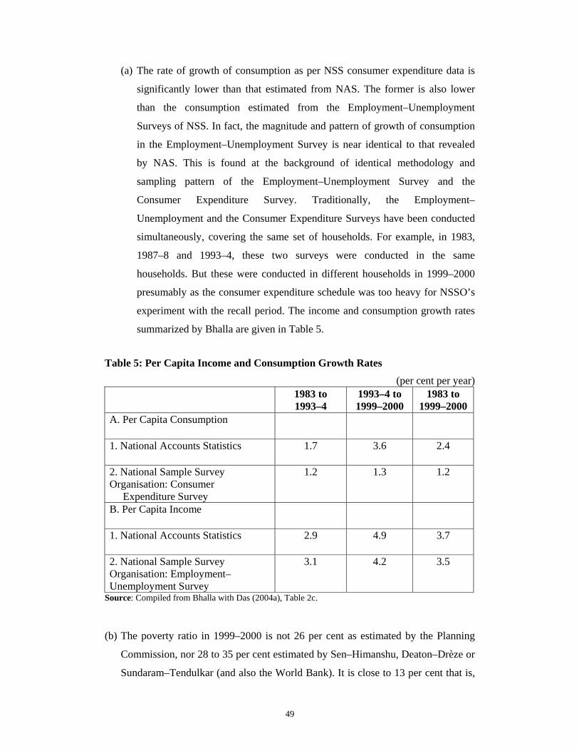
49
(a) The rate of growth of consumption as per NSS consumer expenditure data is
significantly lower than that estimated from NAS. The former is also lower
than the consumption estimated from the Employment–Unemployment
Surveys of NSS. In fact, the magnitude and pattern of growth of consumption
in the Employment–Unemployment Survey is near identical to that revealed
by NAS. This is found at the background of identical methodology and
sampling pattern of the Employment–Unemployment Survey and the
Consumer Expenditure Survey. Traditionally, the Employment–
Unemployment and the Consumer Expenditure Surveys have been conducted
simultaneously, covering the same set of households. For example, in 1983,
1987–8 and 1993–4, these two surveys were conducted in the same
households. But these were conducted in different households in 1999–2000
presumably as the consumer expenditure schedule was too heavy for NSSO’s
experiment with the recall period. The income and consumption growth rates
summarized by Bhalla are given in Table 5.
Table 5: Per Capita Income and Consumption Growth Rates
(per cent per year) 1983 to
1993–4 1993–4 to 1999–2000
1983 to 1999–2000
A. Per Capita Consumption
1. National Accounts Statistics 1.7 3.6 2.4
2. National Sample Survey Organisation: Consumer Expenditure Survey
1.2 1.3 1.2
B. Per Capita Income
1. National Accounts Statistics 2.9 4.9 3.7
2. National Sample Survey Organisation: Employment–Unemployment Survey
3.1 4.2 3.5
Source: Compiled from Bhalla with Das (2004a), Table 2c.
(b) The poverty ratio in 1999–2000 is not 26 per cent as estimated by the Planning
Commission, nor 28 to 35 per cent estimated by Sen–Himanshu, Deaton–Drèze or
Sundaram–Tendulkar (and also the World Bank). It is close to 13 per cent that is,

50
half the official estimate made by the Planning Commission and about one-third
the World Bank estimate.
(c) The rate of economic growth accelerated after the institution of major economic
reforms in the early 1990s (July 1991). This acceleration is apparent in the
growth of per capita Gross Domestic Product (GDP), from 3 per cent in the 1980s
to around 4.5 per cent in the 1990s. It is also evident in the growth in per capita
consumption of NAS and that obtained from the Employment– Unemployment
Survey of NSS.
(d) The effect of inequality on poverty reduction is small; about one-tenth of the
reduction in poverty is due to changes in inequality and the remaining nine-tenth
due to growth. Growth accelerated in the 1990s with near constant inequality. The
only negative feature of the Indian economy in the 1990s is low growth of
employment. The rate of employment generation, which was 3.1 per cent per year
in the 1980s, lowered to 1.4 per cent per year in the 1990s.
(e) Real wages accelerated from 2.4 per cent per annum in the 1980s (1983 to 1993–
4) to 4.5 per cent per annum in the 1990s (1993–4 to 1999–2000). Thus, the
growth in real wages per worker in the 1990s is nearly twice that in the 1980s.
This increase in wages did not bypass the poor. The annual growth of (i) rural
wages accelerated from 2.4 per cent in the 1980s to 4.3 per cent in the 1990s, and
(ii) wages of agricultural workers (in the rural areas) increased from 2.2 per cent
in the 1980s to 3.1 per cent in the 1990s. From these, Bhalla concludes that in the
1990s, real wages accelerated and unemployment rates declined. He also states
that these growth rates estimated from the wages data collected in the
Employment–Unemployment Survey of NSS are orthogonal to the view that the
growth in agricultural wages decelerated in the 1990s. The growth rate of wages is
summarized in Table 6.
(f) The annual rate of growth in wages was 3.1 per cent in rural areas and 3.2 per cent
in urban areas from 1983 to 1999–2000. This strongly suggests unchanged
inequality. Together, these have impacted reduction in poverty.

51
Table 6: Growth Rate of Wages in Rural Areas
(per cent per year)
1983 to 1993–4
1993–4 to 1999–2000
1983 to 1999–2000
A. From NSS Employment– Unemployment Survey data
1. Real Wages per Worker 2.4 4.5 3.2 2. Wages in Rural Areas 2.4 4.3 3.1 3. Agricultural Workers Wages: Rural Areas
2.2 3.1 2.5
B. Ministry of Agriculture 1. Agricultural Wages of India (AWI) 4.1 2.8 3.6 2. Cost of Cultivation Survey 2.8 4.5 3.5 C. NCAER Survey: Rural Income 3.3
Note: The NCAER income calculations are based on the panel survey of rural households conducted by NCAER in 1970–1, 1980–1 and 1998–9. The growth rate from these data has been computed by Foster–Rosenzweig. The rural income includes both wage and non-wage. The growth rates relate to the period 1981 and 1998. Source: Compiled from Bhalla with Das (2004a), Table 2c.
(g) Using NSS consumer expenditure data of 38th and 50th Round and NAS
consumption of the year, Bhalla estimates the poverty ratios as 45 per cent in 1983
and 27.3 per cent in 1993–4. Bhalla, as mentioned earlier, participated in the
debate on the comparability of NSS 55th Round consumer expenditure data and
also on the poverty estimates made from these data. But, he does not use NSS
55th Round consumer expenditure data at all to estimate poverty for the
year 1999–2000. Instead, he uses some parameters of NSS 38th Round (1983)
consumer expenditure data and the data from the Employment–Unemployment
Surveys of NSS to estimate the poverty ratio in 1999–2000 as 13.3 per cent.
(h) The official estimates of poverty, made by the Planning Commission from the
consumer expenditure survey of NSS work out to 44.5 per cent in 1983, 36.0 per
cent in 1993–4 and 26.1 per cent in 1999–2000. Thus, Bhalla estimates the
poverty reduction during the period 1983 to 1999–2000 as 32 percentage points as
against 18.4 percentage points of the Planning Commission.
The poverty ratio estimated by Bhalla is compared with that of the Planning
Commission in Table 7. The rate of decline in poverty ratio in the 1980s (1983 to

52
1993–4) and 1990s (1993–4 to 1999–2000) realized by Bhalla is more than twice of
that of the Planning Commission.
Table 7: Poverty Ratio: Bhalla and Planning Commission
Bhalla Planning Commission A. Poverty Ratio 1. 1983 45.0 44.5 2. 1993–4 27.3 36.0 3. 1999–2000 13.3 26.1 B. Rate of Decline (% p.a.) 1. 1983 to 1993–4 4.65 2.00 2. 1993–4 to 1999–2000 11.29 5.22 3. 1983 to 1999–2000 7.12 3.18
5.2 Poverty, Inequality and Growth: The Relationships
Bhalla addresses three questions for a comprehensive evaluation of the poverty–
inequality–growth nexus. These are: (a) the relationship between growth and poverty
reduction, that is, the changes in poverty ratio as a result of a given magnitude of
growth in income, (b) relationship between inequality and growth, and (c) relationship
between growth and initial level of inequality, or precisely, what would have been the
state of growth for the initial level of inequality.
Reduction in poverty, given the growth rate and assuming unchanged inequality, is
non-linear. The rate of poverty reduction, ceteris paribus, depends on the clustering of
the poor around the poverty line. The reduction in the poverty ratio per unit of growth
is termed as the ‘shape of distribution’ elasticity by Bhalla. For NSS consumption
distribution, and poverty levels around 25 to 40 per cent, he estimates the national
average value of the (shape of distribution) elasticity as 0.85. It implies that for 1 per
cent growth in per capita consumption, the poverty ratio should decline by 0.85
percentage points, ceteris paribus.
Bhalla calculated the trend in inequality from the quintile shares of per capita wage
incomes yielded by NSS Employment–Unemployment Surveys of 1983 (NSS 38th
Round), 1993–4 (NSS 50th Round) and 1999–2000 (NSS 55th Round). He estimates
the annual growth rates for the different quintiles in the 1990s as: 5.4 per cent for the

53
richest quintile and 3.7 per cent for the poorest quintile. The per capita income of the
individuals located in the middle three quintiles (that is, 20th to 80th percentiles)
increased by 2.4 to 2.9 per cent per year. The Gini index of wage income turns out to
be highly unequal and rising; it increased from 0.4644 in 1993–4 to 0.5023 in 1999–
2000; but, the log variance index declined from 1.03 to 0.87. However, it should be
noted that these represent wage-inequality and not income-inequality and also that
these are estimated from the Employment–Unemployment Survey and not Consumer
Expenditure Survey. The limitations of the wage data gathered in the Employment–
Unemployment Survey are well known. In this context, the results of Bhalla’s study
on growth, equity and poverty are summarized.
The growth in per capita consumption derived from the Consumer Expenditure
Surveys of NSS averaged 1.1 per cent per year during the period 1983 to 1999–2000.
In contrast, other survey estimates, namely, Employment–Unemployment Survey of
NSS, Income and Consumption Survey of NCAER, Agricultural Wages and Crop
Cultivation Surveys (of the Ministry of Agriculture, Government of India) indicate
that the wages of the poorest, e.g., the agricultural workers, increased by 2 to 2.4 per
cent in the 1980s and more than 3 per cent per year in the 1990s. For rural workers,
the average growth rate estimated from the Employment–Unemployment Survey of
NSS works out to 2.4 per cent per year in the 1980s and 4.3 per cent per year in the
1990s.
The estimates of inequality, measured from NSS consumer expenditure data vary by
method, definition of consumption and choice of price deflator. The adjusted
distribution (adjusted for price differential) shows a decline in inequality in the 1980s
(1983 to 1993–4) and more in the 1990s (1993–4 to 1999–2000).
The above growth in consumption/income and the stable inequality is certain to result
in a decline in poverty. If a correct survey based minimum estimate of growth is
applied to NSS consumption distribution for 1983, the poverty ratio in 1999–2000 as
per Bhalla’s calculation becomes, 13 per cent.

54
The only black spot of this ‘high growth low poverty’ syndrome in the 1990s is the
slower growth in employment, which is 1.4 per cent per year as compared to 3.1 per
cent per year realized in the 1980s.
5.3 The View of 1983–2000
Before spelling out his own ideas about the nexus between growth, equity and poverty
during the period 1983 to 1999–2000, Bhalla summarizes the views of others, for
example, Sundaram–Tendulkar, Deaton, Deaton–Drèze and Sen–Himanshu. The
summary view can be arranged in the following four points.
(a) The growth rate of agriculture declined from 3.7 per cent per year in the 1980s
(1983 to 1993–4) to 2.6 per cent per year in the 1990s (1993–4 to 1999–2000).
(b) The growth rate of real wages in agriculture declined from about 5 to 5.5 per
cent per year in the 1980s to 2.5 per cent per year in the 1990s. Because
agricultural households constitute the poorest of the poor, this lowering of the
growth rate of income in the 1990s may indicate rise in poverty.
(c) The per capita consumption differential between urban and rural areas
increased significantly over time.
(d) The growth in the poorer states lagged behind the richer states, indicating
increasing inequality. The decline in the incidence of poverty (estimated from
NSS consumer expenditure data) was slower in the 1990s; it is 8 per cent
points in the 1980s as compared to five percentage points in the 1990s.
This slower decline in poverty in the 1990s (conclusion of Sen–Himanshu), according
to Bhalla is not consistent with the acceleration of economic growth. The changed
pattern of growth in the 1990s caused by the economic reforms that began in the early
1990s (that is, the economic reform programmes initiated by the Government of India
at the height of economic crisis in July 1991) was responsible for the slower decline
in poverty and change in inequality. It is against this backdrop that Bhalla re-writes
the poverty scenario in the country in the following manner.

55
(a) The annual rate of economic growth averaged more than 5.5 per cent during
the period 1980 to 2004 (measured from NAS). The same in per capita
terms averaged 2.9 per cent in the 1980s and 4.9 per cent in the 1990s.
(b) Consumption growth as per NSS consumer expenditure data is lower than that
of the Employment–Unemployment Survey and also of NAS. The annual rate
of growth of per capita NAS consumption is 1.7 per cent per year in the 1980s
and 3.6 per cent per year in the 1990s. The per capita consumption from NSS
for the corresponding period is 1.2 per cent per year and 1.3 per cent per year
respectively. From the Employment–Unemployment Survey of NSS, the
annual rate of growth of income is estimated as 1.1 per cent in the 1980s and
3.1 per cent in the 1990s.62 Hence the conclusion: the growth of NSS
consumption, which is used by the Planning Commission (and many others) to
estimate poverty, is the least; it is 1.2 per cent per year; and, increase in per
capita consumption in the 1990s is greater than that in the 1980s. He
emphasizes that NSS consumption understates not only the consumption
growth of all population but also of the poor.
(c) The use of longer (365-day) recall period for five non-food items, namely,
clothing and textiles, footwear, durable goods, education and institutional
medicine in NSS 55th Round Consumer Expenditure Survey impacts on the
inter-relations between growth, equity and poverty. The inequality in the class
distribution of consumption decreases when 365-day recall period is used for
the five non-food items. Because of the low frequency of purchase of these
five items, they are more likely to get recorded on an annual rather than
monthly basis. Consequently, at any point in time, per capita consumption will
be higher from the use of 365-day recall periods as against 30-day recall
period. This higher consumption leads to a lower poverty ratio.63 This changed
method of collecting information on low frequency items, that is, using 365-
day and not both 30- and 365-day recall periods, in all probability affects the
variance of per capita consumption. As an illustration, he points out the
consumption expenditure in education, which are mostly undertaken (and 62 In the 1983 and 1993–4 surveys (NSS 38th and 50th Rounds respectively) the data on Employment–
Unemployment and Consumer Expenditure were gathered from the same households. But, in 1999– 2000 (NSS 55th Round), these were collected from different households.
63 Also shown by others, for example, Deaton, Sundaram–Tendulkar and Sen–Himanshu.

56
remembered) on a monthly basis. The consumption data gathered from 365-
day recall period for education may be conniving along with the consumption
of 30-day recall period. The absence of 30-day recall period for these five non-
food items in NSS 55th Round may mean that the consumption from 365-day
recall period might get understated in 1999–2000 relative to 1993–4, when
both 30-day and 365-day recall periods were used. Its outcome though is a
certain underestimation of consumption in 1999–2000. These, however,
should not matter for Bhalla, for he estimates the poverty ratio in 1999–2000
without using NSS 55th Round consumer expenditure data in any manner.
5.4 Poverty Estimation: The Approach
Bhalla estimated poverty ratio for three points of time, namely, 1983, 1993–4 and
1999–2000. From these, he estimated the trend of poverty reduction during the period
(a) 1983 to 1993–4 (b) 1993–4 to 1999–2000, and (c) for the entire period 1983 to
1999–2000. It has already been mentioned that Bhalla equated the period (a) with
1980s and (b) with 1990s.
Bhalla relies on NAS consumption to estimate poverty. Along with this, he makes use
of NSS consumer expenditure data of the 38th and 50th Rounds to estimate the
poverty ratio in 1983 and 1993–4 respectively. Significantly, he does not use NSS
55th Round consumer expenditure data to estimate the poverty ratio for the year
1999–2000, though he dwells on the comparability issue and makes considerable
effort to demonstrate that: (a) the food consumption in NSS 55th Round is not biased
(that is, neither overestimated nor underestimated), and (b) the non-food consumption
is underestimated. The manner and method by which Bhalla addresses the
comparability of NSS 55th Round consumer expenditure data with its earlier rounds,
which is the bone of contention, is described first. Then the technique employed by
him to derive the poverty ratio in 1999–2000 is described.
5.4.1 Comparability Issues in NSS 55th Round Consumer Expenditure Data
The loss of comparability of NSS 55th Round (1999–2000) consumer expenditure
data with its earlier rounds as already noted, arises from: (a) alleged contamination of

57
food consumption data, due to the use of both 7-day and 30-day recall periods from
the same households and (b) use of only 365-day recall period to collect consumption
data of five non-food items. Bhalla’s view on these two issues is described below.
Food Consumption: Bhalla states that the food consumption in NSS 55th Round
would not have been contaminated (or suffered from upward or downward bias due to
the simultaneous presence of 7-day and 30-day recall periods) if the field investigators
had collected the consumption data from 30-day recall period first. The situation at
the ground level seems to defy this. As Sundaram–Tendulkar note: The initial
instructions to NSSO (National Sample Survey Organisation) field staff did not
explicitly mention the sequence in which information from respondents was to be
elicited for the two recall periods (7-day and 30-day). Nearly one-and-a-half months
after the field work was launched for NSS 55th Round, on the 19th August, 1999 a
communication from the Sampling Design and Research Division (SDRD) of NSSO,
directed the investigators to elicit information first for the 30-day recall for all items
of the food group and then to seek the same (again from the beginning) for the last 7
days. Which sequence was followed remains an open question.64 This doubt of
Sundaram–Tendulkar is echoed in the field visits of Jean Drèze. Drèze, from his
discussions with a number of NSSO investigators in parts of Rajasthan and Uttar
Pradesh reported that the field investigators had canvassed the 7-day schedule first
and the 30-day schedules later.65 Bhalla cites two evidences to support the contention
that food consumption in NSS 55th Round (1999–2000) is not biased, that is, neither
an overestimate nor an underestimate.
Evidence I: Food consumption of NSS 55th Round (1999–2000) is compared with
those gathered in the consumer expenditure data of NSS 56th Round,66 which relates
to the year 2001-02. This data (NSS 56th Round) is free from such recall period
problem. The food consumption of 1999–2000, which is available only in nominal
terms,67 is converted into real terms using food price index of the industrial workers
(that is, Food Index of the Consumer Price Index of Industrial Workers, CPIIW). Real
64 Page 337, Sundaram and Tendulkar (2003a).
65 Page 1387, Sundaram and Tendulkar (2003c).
66 This is from the ‘thin’ sample of NSS, as opposed to the large sample of 1999–2000. 67 For that matter all NSS consumption estimates are available only in nominal terms and not in real
terms from NSSO.

58
food consumption in 1999–2000 (which is allegedly overestimated) is found to be
approximately the same as in 2000–1, 1993–4 and in 1987–8. From this, Bhalla
contends that if per capita food consumption has stayed more or less constant, and if
the observed food consumption in 1999–2000 is the same as in 1987–8, 1993–4 and
2000-01, there is little reason to believe that the consumption in 1999–2000 was
overestimated ‘in other than a most marginal manner’. And hence the conclusion: no
overestimation of food consumption in 1999–2000 due to the simultaneous presence
of 7-day and 30-day recall periods questions.
It may be pertinent to note that such a conclusion is extremely sensitive to the choice
of the price index, which is used to convert nominal consumption into real
consumption. The conclusion may alter if the food price index of the Consumer Price
Index of Industrial Workers (which has been used to convert nominal consumption
into real consumption) is replaced by the food index of the Consumer Price Index of
Agricultural Labourers, CPIAL or the food price index implicit in the private
consumption of NAS.
Evidence II: Bhalla’s second evidence relies on the calculations of Sundaram–
Tendulkar, who compared food and other consumption of NSS Consumer
Expenditure Survey with analogous expenditures in the Employment–Unemployment
Survey. For non-food items, Sundaram–Tendulkar found under-reporting of
consumption (the one not subject to 7-day bias) in the Employment–Unemployment
Survey to be of the same order of magnitude (about 10 per cent) as the under-
reporting of food items. From this they concluded that it was unlikely that there was
any aggregate overestimation of food expenditure in the consumer expenditure survey
of 1999–2000. Bhalla cites this as evidence to demonstrate the absence of bias in food
consumption in NSS 55th Round.
Consumption of Five Non-Food Items: Bhalla examined the possibility of bias in the
consumption of the five infrequently purchased non-food items in NSS 55th Round
due to the use of only 365-day recall period. The conclusion he arrived at is: The
absence of 30-day recall period with the 365-day for the five non-food items in NSS
55th Round (that is, in 1999–2000) understates the total consumption by 3 per cent.

59
This, according to Bhalla, is the only source of underestimation of consumption in
NSS 55th Round.
5.4.2 The Poverty Ratios: 1983 to 1999–2000
Bhalla estimated poverty ratio for the years 1983, 1993–4 and 1999–2000. These
estimates have already been reported in Table 7. He used the Planning Commission
poverty lines throughout. The methodology employed by Bhalla to estimate the
poverty ratios in 1983 and 1993–4 is similar. But, the methodology employed for
1999–2000 is different. For this reason, these two methodologies are discussed
separately below.
Poverty Estimates of 1983 and 1993–4: Bhalla estimates the poverty ratios in 1983
and 1993–4 as 45.0 per cent 27.3 per cent respectively. He does not use the
consumption expenditure of NSS alone to estimate poverty for he does not agree that
it can be so less than the consumption of the National Accounts Statistics (NAS) and
also from the consumption derived from the Employment–Unemployment Survey of
NSS. The poverty ratios in these two years are estimated from NSS consumer
expenditure data of the 38th and 50th Rounds respectively after adjusting them pro-
rata to the private consumption of NAS of the year. Since the adjustment of NSS
consumption to NAS consumption is at the heart of the estimate, the procedure is
described below.
Adjustment of NSS Consumption to NAS Level: Poverty is estimated from a
consumption level, which is a marriage of consumption derived from the Consumer
Expenditure Survey of NSS and that of NAS. This marriage is solemnized by
adjusting the average consumption of NSS to that of NAS, at a fairly disaggregated
level (for 39 items/commodity groups). The method of deriving an adjusted
distribution by matching commodity-specific average consumption of NSS with the
corresponding NAS consumption, being central to the methodology of poverty
estimation by Bhalla, may be outlined.
The average consumption from NAS and NSS is worked out for different
items/groups (39 in all). From these, the ratio of NAS to NSS average consumption is

60
calculated. NSS consumption (assumed to be underestimated) is adjusted to NAS
level of consumption. The adjustment is made item-wise in the following way.
For each individual, an average multiplier is worked out as the ratio of the adjusted
sum of individual and item-specific consumption, to the sum of consumption in NSS.
Therefore, the underestimation of consumption is estimated not only at the
commodity level, but also at the individual level. A bold step, no doubt! Some
empirics are: The underestimation in consumption in 1993–4 (NSS 50th Round)
ranges from a minimum of 11 per cent for cereals to a maximum of 150 per cent for
clothing and footwear.68
The average multiplier is thus obtained for each household and for each decile of
households. The multiplier is different for each individual and is a function of the
consumption pattern. The new consumption distribution is computed by adjusting
NSS consumption with the multipliers. This is done for each of the years for which he
estimated poverty from NSS consumer expenditure data (that is, NSS 38th and 50th
Rounds). The results are: for the poorest deciles, the average underestimation (of NSS
consumption) is 30 per cent. The multiplier rises progressively with the expenditure
of the households. For the first eight deciles it is narrow; in the range of 50 to 60 per
cent in 1993–4. The multiplier for the fourth decile (approximately equated with the
poverty line class) is 1.25 in 1983 with the average multiplier being 1.29; for 1993–4
the multiplier for the fourth decile is 1.55 with the national average being 1.62. The
underestimation of food items (42 per cent) is considerably less than the
underestimation of non-food items (68 per cent).
5.4.3 Poverty Estimate in 1999–2000
Bhalla does not make use of NSS 55th Round consumer expenditure data at all to
estimate the poverty ratio in 1999–2000. Instead, he uses NSS data on wages of casual
workers in rural areas to estimate consumption in 1999–2000, from which he
estimated poverty in that year. The manner and method employed by Bhalla to
estimate the poverty ratio in 1999–2000, along with the empirics is described below.
68 The NSS cereals consumption in 1993–4 was Rs. 79.3 compared to the Rs. 87.8 in NAS implying
that each individual’s consumption of cereals is underestimated by 10.7 per cent in NSS.

61
The growth of nominal wages in rural areas between 1983 and 1999–2000 is set as 11
per cent per year. The annual price inflation during this period is calculated as 8.1 per
cent. From these, the growth of real wage works out to 2.9 per cent per annum. The
nominal wages are obtained directly from NSS data. The inflation rate during the
period 1983 to 1999–2000 is calculated in two stages: (a) for the period 1983 to
1987–8 and (b) for the period 1987–8 to 1999–2000. The inflation rate for the first
stage (1983 to 1987-8) is computed from the price indices employed by the Planning
Commission to update its poverty lines for the period 1983 to 1987–8. The inflation
rate for the second stage (1987-8 to 1999-2000) is equated with that implicit in
Deaton–Tarozzi price indices for the period 1987–8 to 1999–2000.
The price deflator plays an important role in converting the nominal wage growth
derived from NSS data into real terms. This makes it necessary to describe the
empirics of the construction of the price deflator computed and used in this regard.
The annual inflation rate (for the period 1987–8 to 1999–2000) based on the price
indices developed by Deaton–Tarozzi (2000) and Deaton (2003b) from NSS unit
record data is 7.6 per cent in rural areas and 8.2 per cent in urban areas. Since Deaton
does not report price indices for 1983, the price deflator for the period 1983 to 1987–8
used by the Planning Commission (which is 7.9 per cent in rural areas and 8.3 per
cent in urban areas) is grafted onto the Deaton price indices for 1987–8, 1993–4 and
1999–2000. This way, the inflation during the period 1983 to 1999–2000 works out to
8.1 per cent per annum in rural areas.
The growth of real wages in rural areas by 2.9 per cent per annum estimated above is
scaled down by Bhalla to 2.5 per cent per year, based on analogous data. With the
assumption of zero savings, increase in wages is equated with increase in
consumption. Allowing 2.5 per cent increase annually for sixteen and half years
covering the period, 1983 to 1999–2000, the average real per capita consumption in
1999–2000 becomes about 51 per cent more than that in 1983. This level of per capita
consumption in 1999–2000 (which is 51 per cent more than that in 1983) coupled
with the 1983 consumption distribution of NSS and the poverty lines of the Planning
Commission yields the poverty ratio in 1999–2000 as 13.3 per cent. This is Bhalla’s
estimate of poverty in 1999–2000 and it is no more than half of the official estimate of
poverty made by the Planning Commission.

62
Bhalla offers upper and lower bound of the estimate of poverty made above. The
details of the derivation are not narrated, as these are functional to the wage data and
the price deflator. The upper bound of the estimate is 15 per cent. The lower bound,
which is based on a conservative estimate of wage growth, indicates the poverty ratio
in 1999–2000 as 12 per cent.
The Comparability Problem: The poverty ratios estimated by Bhalla for the years
1983 and 1993–4 are comparable since these are derived from identical methods, that
is, adjusting NSS consumer expenditure distribution to the level of NAS consumption.
But, the poverty ratio in 1999–2000 estimated as 13.3 per cent cease to be comparable
with those of 1983 estimated as 45 per cent because of the difference in the
methodology of estimation and also of data use. For this reason, the poverty ratio of
1999–2000 should not be used to measure the magnitude of poverty reduction during
this period. This remains one major constraint of using the poverty estimates derived
by Bhalla.
An identical situation is encountered with the comparison of the poverty estimates of
1993–4 and 1999–2000. But, it does not alter the conclusions in a substantial measure
since the poverty ratio in 1993–4 based on the methodology employed for poverty
estimation in 1999–200069 is close to the estimate obtained from adjusting NSS
consumption distribution to NAS level.
Why the poverty ratio in 1999–2000 is not estimated following the method employed
for 1983 and 1993–4, that is, by adjusting NSS consumption distribution of the 55th
Round to NAS level of consumption of the year and then estimate the percentage of
persons lying below the poverty line from this adjusted distribution. The reason may
be: the aggregate NAS consumption is 77 per cent more than the aggregate NSS
consumption and the resulting poverty ratio is less than 4 per cent. The debate might
not have taken off with such a low level of poverty in 1999–2000.
Bhalla’s use of the wages of casual workers on the grounds that these are the wages of
agricultural workers, who occupy the least-skilled jobs and lowest paid workers in the 69 Estimating the poverty ratio in 1993–4 from annual growth of income of the poor by 2.2 per cent
during the period 1983 to 1993–4 and NSS 38th Round consumption distribution (1983).

63
country, may be tenable. But, the sufficiency of using NSS wage data for reasons of
similarity in the rate of growth of nominal wages of NSS and Agricultural Situation in
India (ASI) during the period 1983 to 1999–200070 is equally untenable because of
the fact that the wage rate is derived from surveys, which are not comprehensive
income surveys, since only limited data are available for the households who are
engaged in business or self-employment. This renders the use of NSS wage data to
compute the consumption level, and ultimately poverty ratio that is computed from it,
disputed. Also, the average wage represented by the mean value (of the wage) is not
adequately reliable, for the presence of large number of outliers in the data. Bhalla,
however, tries to tackle this issue by using the median wage, which is less
contaminated by outliers.
5.5 Exchanges with Deaton The exchanges between Bhalla and Deaton make interesting reading though the
methods employed by them are unrelated in all respects and their results almost hit the
opposite poles.
5.5.1 Bhalla on Deaton
Deaton’s 30-day goods (fuel and light, non-institutional medical services, toilet
articles, rent, consumption of miscellaneous goods and services, etc.) are the only
group of consumption items whose definition had stayed the same for all the surveys.
The consumption, and then the inequality and poverty in 1999–2000 can be obtained
by suitably blowing up this consumption. These 30-day goods, which contain 20 to 30
per cent of total consumption, are in virtually every consumer’s budget and are
heterogeneous with high-income elasticity. These underline the importance of 30-day
goods in Deaton’s method.
As Deaton states, use of 30-day goods are theoretically justified if two conditions
hold. First, that the magnitude and distribution of the expenditure on these goods are
70 During the period 1983 to 1999–2000, the rate of growth based on ASI data is 11.5 per cent per annum; from NSS data it works out 11 per cent per year for males and 10.8 per cent per year for females.

64
not affected by the presence or absence of questions in other non-30-day goods part of
the questionnaire. Second, that the relationship between the consumption of 30-day
goods and total consumption (strictly, the log of the consumption) is the same in the
year of adjustment (1999–2000) as the base year used for adjustment (1993–4). These
assumptions are rational since tastes and relative prices are unlikely to change in the
span of six years, 1993–4 to 1999–2000.71
With these two assumptions, the observed relationship between total consumption and
the consumption on 30-day goods can be imposed on the data for 30-day goods in
other years. The data for 30-day goods are not contaminated and hence reliable
(unlike the data on food consumption). The estimate of consumption based on this
method is, therefore, comparable with earlier years.
Deaton accepted the likelihood of overestimation of consumption in NSS 55th Round
(as a joint outcome of the contamination of food consumption data and absence of 30-
day recall period in the case of five non-food items), and his results show some rise in
poverty after correcting for this (Deaton’s method yield poverty ratio in 1999–2000 as
28.5 as against the Planning Commission estimate of 26.1 per cent from NSS 55th
Round data).
The above makes it explicit that Bhalla is not critical of Deaton’s method. At the same
time, Bhalla’s choice of the method to estimate poverty in 1999–2000 is nowhere near
it. While Deaton’s method reveals the likelihood of overestimation of consumption in
NSS 55th Round, Bhalla goes the other way and shows underestimation of
consumption. According to Bhalla, the total consumption in NSS 55th Round is
underestimated by 3 per cent.
Bhalla may not have anything against Deaton’s method theoretically; he cannot
accept the results that accompany it either. For, Bhalla is not willing to accept a level
of poverty in 1999–2000, which is beyond the range of 12 to 15 per cent and the
magnitude of decline in poverty ratio between 1983 and 1999–2000, which is less
than 32 per cent. Deaton falls far short of Bhalla’s expectations on both counts.
71 This latter assumption though, has vehemently been questioned by Sen–Himanshu.

65
5.5.2 Deaton on Bhalla
Bhalla is one of the most consistent advocates of the position that poverty in India has
declined rapidly in the 1990s and the official estimate of 26.1 per cent in 1999–2000
is a gross overestimate. ‘It is almost incontrovertible that poverty in India was less
than 15 per cent in 1999–2000.’ That is how Bhalla summarizes his stance on poverty.
Bhalla estimates poverty by adjusting NSS consumption to the level of NAS
consumption, ignoring the detailed arguments by Minhas72 against such adjustment,
as those of Kulshreshtha and Kar73 demonstration of the inferiority of the numbers
that Bhalla treats as correct compared with those that he rejects74. Annexure D
summarizes the arguments on NSS-NAS consumption issue, on which Bhalla’s
estimate of poverty is largely based.
Bhalla also argues that inequality has declined in the late 1990s. His argument that
there has been reduction in inequality is based on measures that appear to be taken
directly from the unadjusted 1999–2000 survey (that is, NSS 55th Round Consumer
Expenditure Data as released by NSSO, in which food consumption data is collected
from both 7-day and 30-day recall periods from the same households and the
consumption of five non-food items are collected only from 365-day recall period),
and are compared with similar measures from earlier surveys. But, the unadjusted data
from NSS 55th Round understate measured inequality because of the change in
response periods for the low frequency items such as durables and clothing.75
Bhalla assumes that growth at the mean automatically translates into growth for the
poor, which assumes away one of the main arguments of the anti-globalizers. The use
of either assumption bypasses the poverty debate because the answer is guaranteed
before we undertake any calculations.
72 Minhas (1998). 73 Kulshreshtha and Kar (2004) 74 Deaton and Kozel (2005), Page 18. 75 Deaton–Drèze (2002)

66
However, Deaton–Kozel find Bhalla’s work important, ‘because it represents one of
the poles in the current debate on the Indian poverty number’.76
5.6 The Relevance of Bhalla’s Estimates
The assessment of the impact of economic reforms on poverty, both in its level and
change, is relevant for India. The issue is being debated and Bhalla intervenes in this
lively debate. Much of the planning and development strategy of this country of one
billion plus people would have to be re-written if the State heeds Bhalla’s poverty
numbers. His experiments with poverty numbers are not confined to India alone. In
his estimates of world poverty, Bhalla (2002) has gone the Beatles way. There he has
not only used a famous John Lennon number77 as the title of this publication, but
almost in fulfillment with the famous Artiste’s dream, declared a world free from
poverty.
6 National Level Poverty Estimates: A Round Up National level poverty estimates are worked out in the rural and urban areas. These
have been aggregated for the country as a whole using the population proportion in
the two regions as weights. The cross-section of the poverty estimates by method,
which are the outcome of the efforts to measure comparable poverty estimate in the
context of the debate on the comparability of NSS 55th Round consumer expenditure
data, are given in Table 8.
76 Deaton–Kozel (2005), page 18. 77 Imagine there is no country / It isn’t hard to do so / Nothing to kill or die for / And no religion too.

67
Table 8: Poverty Ratio and Number of Poor Poverty
Ratio Rural
Poverty Ratio Urban
Poverty Ratio Total
No. of Poor Rural
No. of Poor Urban
No. of Poor Total
A.1 Planning Commission a) 1983 45.7 40.8 44.4 252.0 70.9 322.9 b) 1993–4 37.3 32.4 36.0 244.0 76.3 320.3 c) Decline 8.4 8.4 8.4 8.0 -5.4 2.6 A.2 Sundaram–Tendulkar a) 1983 49.0 38.3 46.5 268.1 65.7 333.8 b) 1993–4 39.7 30.9 37.4 261.4 72.6 334.0 c) Decline 9.3 7.4 9.1 6.7 -6.9 -0.2 B.1 Planning Commission a) 1987–8 39.1 38.2 38.9 231.9 75.2 307.1 b) 1993–4 37.3 32.4 36.0 244.0 76.3 320.3 c) Decline 1.8 5.8 2.9 -12.1 -1.1 -13.2 B.2 Deaton a) 1987–8 39.4 39.1 39.4 233.7 77.0 310.7 b) 1993–4 37.1 32.9 36.0 242.7 77.5 320.2 c) Decline 2.3 6.2 3.4 -9.0 -0.5 -9.5 B.3 Deaton–Drèze a) 1987–8 39.4 22.5 35.2 233.7 44.3 278.0 b) 1993–4 33.0 17.8 29.0 215.9 41.9 257.8 c) Decline 6.4 4.7 6.2 17.8 2.4 20.2 B.4 Sen–Himanshu a) 1987–8 35.2 34.9 35.2 208.8 68.7 277.5 b) 1993–4 31.9 28.0 30.9 208.7 65.9 274.6 c) Decline 3.3 6.9 4.3 0.1 2.8 2.9 C.1 Planning Commission a) 1993–4 37.3 32.4 36.0 244.0 76.3 320.3 b) 1999–2000 27.1 23.6 26.1 193.2 67.0 260.2 c) Decline 10.2 8.8 9.9 50.8 9.3 60.1 C.2 Deaton a) 1993–4 37.1 32.9 36.0 242.7 77.5 320.2 b) 1999–2000 30.0 24.7 28.5 213.9 70.1 284.0 c) Decline 7.1 8.2 7.5 28.8 7.4 36.2 C.3 Deaton–Drèze a) 1993–4 33.0 17.8 29.0 215.9 41.9 257.8 b) 1999–2000 26.0 12.0 22.2 185.4 34.1 219.5 c) Decline 7.0 5.8 6.8 30.5 7.8 38.3 C.4 Sundaram–Tendulkar a) 1993–4* 37.9 28.8 35.5 249.4 67.7 317.1 b) 1993–4 34.2 26.4 32.2 225.3 62.1 287.4 c) 1999–2000 28.9 23.1 27.3 210.5 63.8 274.3 d) Decline 5.3 3.3 4.9 14.8 -1.7 13.1 C.5 Sen–Himanshu a) 1993–4 31.6 27.9 30.6 206.7 65.7 272.4 b) 1999–2000 28.8 25.1 27.8 205.3 71.3 276.6 c) Decline 2.8 2.8 2.8 1.4 -5.6 -4.2
Note: The negative sign indicate increase in the poverty ratio/number of poor. The number of poor is in millions. * Sundaram–Tendulkar’s original estimate. This was corrected in (b).

68
6.1 The Planning Commission Estimates and its Alternatives
There are, in all, five estimates of the poverty ratio for 1999–2000, measured as
alternatives to the official estimates made by the Planning Commission. These
originate from: (i) Deaton (ii) Deaton–Drèze (iii) Sundaram–Tendulkar (iv) Sen–
Himanshu and (v) Bhalla. Four of these five estimates (Bhalla being the sole
exception) are derived from NSS consumer expenditure data of the large sample
survey and are born out of the attempts to make NSS 55th Round consumer
expenditure data comparable with the earlier rounds. These four estimates are
compared here, along with the Planning Commission estimate because these are all
derived from NSS consumer expenditure data and their differences lie in the approach
to make NSS 55th Round consumer expenditure data comparable with the earlier
rounds.
(a) Planning Commission: The Planning Commission poverty ratio is estimated
from the consumer expenditure data of NSS 55th Round as published by the
NSSO. This is the official estimate of poverty in the country. The Planning
Commission’s use of NSS 55th Round consumer expenditure data to estimate
poverty in 1999–2000 is the epicenter of the debate. The Planning
Commission estimates of the poverty ratio are given in A.1, B.1 and C.1 in
Table 8.
(b) Deaton: The poverty estimates made by Deaton are: (i) The poverty ratio in
1987–8 is based on URP consumption (30-day recall period for all items). (ii)
The poverty ratio in 1993–4 is based on MRP consumption (365-day recall
period for five non-food items and 30-day recall period for the remaining
items); (iii) The poverty ratio in 1999–2000 is estimated from NSS 55th
Round consumer expenditure data, in which the food consumption is freed
from contamination using Deaton method. Planning Commission poverty lines
are used to derive these poverty estimates. Deaton’s estimates of the poverty
ratio are given in B.2 and C.2 in Table 8.
(c) Deaton–Drèze: The poverty estimates made by Deaton–Drèze are identical to
that of Deaton, except the fact that it uses poverty lines, derived from Deaton–
Tarozzi price indices, and not the Planning Commission poverty lines. The

69
difference between the poverty estimates of Deaton and Deaton–Drèze thus
indicate the impact of change in the money value of the poverty line. Deaton–
Drèze estimates of the poverty ratio are given in B.3 and C.3 in Table 8.
(d) Sundaram–Tendulkar: The money value of the poverty lines used by
Sundaram–Tendulkar is different from that of the Planning Commission. They
updated the national rural and urban poverty lines (1973–4) of the Planning
Commission by the price inflation measured by the Consumer Price Index of
Agricultural Labourers (CPIAL) and Consumer Price Index of Industrial
Workers (CPIIW) respectively and used them to estimate poverty. Sundaram–
Tendulkar estimate of the poverty are: (i) The poverty ratio in 1983 is based
on URP consumption (30-day recall period for all items). (ii) No estimate of
poverty in 1987–8. (iii) Prepared three estimates of the poverty ratio in 1993–
4, one from URP consumption and two from MRP consumption. (iv) The
poverty ratio in 1999–2000 is estimated from MRP consumption (365-day
recall period for five non-food items and 30-day recall period for the
remaining items). Sundaram–Tendulkar tested NSS 55th Round food
consumption data derived from 30-day recall period for possible
contamination but found none. Sundaram–Tendulkar estimates of the
poverty ratio are given in A.2 and C.4 in Table 8. The poverty estimates made
by Sundaram–Tendulkar can be used to measure the change in the poverty
ratio and in the number of poor for the period 1983 to 1993–4 and also for the
period 1993–4 to 1999–2000. But, these cannot be used to measure the change
for the entire period 1983 to 1999–2000.
(e) Sen–Himanshu: Sen–Himanshu estimates of the poverty ratios are given in
B.4 and C.5 in Table 8. (i) The poverty ratio in 1987–8 is based on MRP
consumption (365-day recall period for three non-food items and 30-day recall
period for the remaining items); (ii) The poverty ratio in 1993–4 given in B.4
is based on MRP consumption (365-day recall period for three non-food items
and 30-day recall period for the remaining items). (iii) The poverty ratio in
1993–4 given in C.5 is based on MRP consumption (365-day recall period for
five non-food items and 30-day recall period for the remaining items). (iv) The
poverty ratio in 1999–2000 is based on MRP consumption (365-day recall

70
period for five non-food items and 30-day recall period for the remaining
items); the food consumption in NSS 55th Round is freed from contamination
using Sen–Himanshu method. The poverty ratios in (i) and (ii) are compared
to assess the decline in poverty in the 1980s and those in (iii) and (iv) are
compared to assess the decline in poverty in the 1990s. Sen–Himanshu uses
Planning Commission poverty lines throughout. The poverty estimates made
by Sen–Himanshu can be used to measure the change in the poverty ratio and
number of poor for the period 1987–8 to 1993–4 and also for the period
1993–4 to 1999–2000. But, these cannot be used to measure the change for the
entire period 1987–8 to 1999–2000.
6.2 The Comparison
The poverty ratio and the number of poor given in Table 8 is a snapshot of the range
of the alternative estimates both at a point of time and by methods. The changes in the
poverty ratio and the number of poor for different periods are compared in the light of
the controversy in the level of poverty and the magnitude of its reduction that
accompanies the Planning Commission estimates. The Planning Commission
estimates of poverty are retained as the basis for comparison since it is the official
estimate and is used by the State to allocate food and fund for the poor.
The estimates primarily indicate that excluding Deaton–Drèze’s urban poverty, for
which they used a widely different price index (for updation of the poverty lines) than
the Planning Commission, the range of the estimates is not so wide as to reveal
something extraordinary. This is evident from the period-wise comparisons of the
poverty estimates made below.
(a) 1983 to 1993–4: The decline in the poverty ratio during this period estimated by
Sundaram–Tendulkar (9.1 percentage points) is greater than those of the Planning
Commission (8.4 percentage points).78 Deaton, Deaton–Drèze and Sen–Himanshu do
not estimate poverty in these two years.
78 While comparing it should be remembered that though both the estimates are based on URP
consumptionURP consumption, the money value of the poverty line used by Sundaram–Tendulkar is different from those of the Planning Commission. Sundaram-Tendulkar updates the 1973–4 poverty

71
(b) 1987–8 to 1993–4: There are four estimates of poverty in this period. These are:
Planning Commission, Deaton, Deaton–Drèze and Sen–Himanshu. The poverty
estimates of the Planning Commission, Deaton and Deaton–Drèze are based on URP
consumption (30-day recall period consumption for all items). Sen–Himanshu
estimate of the poverty ratio during this period is based on MRP consumption (365-
day recall period for three infrequently purchased non-food items and 30-day recall
period for the remaining items).
The decline in poverty ratio during this period is least in the Planning Commission
estimate (2.9 percentage points). The difference between Deaton and Planning
Commission estimates is marginal (whereas these two estimates should have been
identical because Deaton uses the Planning Commission poverty line and NSS
consumer expenditure data of similar recall period), arising from the fact that the
latter are extrapolated from consumption distribution published by NSSO by
expenditure groups whereas the former are directly calculated from the unit record
data. The money value of the poverty line used by Deaton–Drèze is different in these
two years. The difference between the Planning Commission and Deaton–Drèze
estimates and for that matter, between Deaton and Deaton–Drèze estimates is due to
the change in the money value of the poverty line. And, the impact of this change in
the money value of the poverty line is significant on poverty reduction, particularly in
the rural areas. Deaton–Drèze estimate of poverty reduction during this period, which
is 6.2 percentage points (as against 3.4 percentage points in Deaton), is mainly driven
by the rural poverty reduction of 6.4 percentage points (as against 2.3 percentage
points in Deaton).
In both these years, Sen–Himanshu estimate of the poverty ratio is lower than that of
the Planning Commission; their estimate of the poverty ratio in 1993–4 is 5.1
percentage points less than that of the Planning Commission. But, they estimate a
greater decline in the poverty ratio during this period (4.3 percentage points as
compared to 2.9 percentage points in case of the Planning Commission); it is about
one and a half times of that of the Planning Commission.
lines of the Planning Commission for use in later years using Consumer Price Index of Agricultural Labourers in the rural areas and Consumer Price Index of Industrial Workers in the urban areas.

72
(c) 1993–4 to 1999–2000: There are five estimates of poverty for this period. The
decline in the poverty ratio during this period is highest in case of the Planning
Commission estimate. This decline in poverty ratio, which is 9.9 percentage points
within the six-year period, 1993–4 to 1999–2000, stirred the debate. It was also
alleged that this decline is exaggerated due to two factors associated with the
collection of consumer expenditure data in NSS 55th Round.
Deaton’s estimate indicates that at the national level, three-fourth of the decline in
poverty ratio estimated by the Planning Commission is real; the remaining one-fourth
is an artefact.
Deaton–Drèze estimates of poverty for these two years maintain all the facets of
Deaton’s estimates except that these are born out of a different poverty line. The
difference that emerges from the altered value of the poverty line employed by
Deaton–Drèze is a substantial lowering of the level of urban poverty in both the years.
Sundaram–Tendulkar for quite some time (that is, until Abhijit Sen pointed out the
error in the compilation of some non-food data in NSS 50th Round) estimated the
decline in poverty ratio during this period (1993–4 to 1999–2000) as 8.2 percentage
points, which exceeds four-fifths of the decline estimated by the Planning
Commission. They concluded that the food consumption in NSS 55th Round is not
contaminated (and hence not overstated) and made the non-food consumption in NSS
50th Round comparable to those of the 55th Round (by generating the consumption of
five infrequently purchased non-food items from 365-day recall period and 30-day
recall period for the remaining items) from the unit record data. However, their
estimate of the magnitude of decline reduced from 8.2 to 4.9 percentage points when
they corrected the error in the compilation of non-food consumption, pointed out by
Abhijit Sen. Their originally estimated (that is, the estimate which was not correct,
and was later changed by them) reduction in the number of poor by 42.8 million
during this period (1993–4 to 1999–2000), as a consequence, is corrected to 13.1
million, which is just 30 per cent of their original estimate, turned their original
conclusions upside down.

73
Sen–Himanshu’s estimate of the decline in poverty ratio during this period is the least
and is about one-quarter that of the Planning Commission. They have used the
Planning Commission poverty lines and, therefore, the entire difference between the
two poverty ratios is due to the two factors, namely, (i) likely overestimation of food
consumption in NSS 55th Round due to contamination, and (ii) use of 365-day recall
period to gather the consumption of five non-food items in NSS 55th Round.
6.3 Impact of Recall Period of Five Non-Food items on Poverty
The Planning Commission estimated the poverty ratio in 1993–4 as 36 per cent. This
is estimated from URP consumption (30-day recall period for all the items) of NSS
50th Round. Sen–Himanshu estimated the poverty ratio in 1993–4 as 30.6 per cent.
This is estimated from the MRP consumption (365-day recall period for five
infrequently purchased non-food items and 30-day for the remaining items) of NSS
50th Round. Both Sen–Himanshu and Planning Commission use the same poverty
line. Therefore, the use of 365-day recall period in place of 30-day recall period for
the five non-food items lowers the poverty ratio in 1993–4 by 5.4 percentage points.
This, therefore, is the impact of the altered recall period of the five non-food items on
the poverty ratio of 1993–4.
It can now be said that the overwhelming impact of recall period of these low
frequency non-food consumption items on the average consumption and on the
inequality in its distribution was unclear to almost everyone. The Planning
Commission noted that the official estimates of poverty for 1999–2000 made from the
consumption expenditure derived from a different methodology (that is, collecting
consumption data of five infrequently purchased non-food items from 365-day recall
period as against 30-day in the past) may not be fully comparable with the earlier
estimates. As is demonstrated below that the impact of the difference in the recall
period of these five non-food items on consumption, both average and its class
distribution, is far greater on poverty than the contamination issue.

74
6.4 Impact of Contamination of Food Data on Poverty
The Planning Commission, from NSS 55th Round consumption data estimated the
poverty ratio in 1999–2000 as 26.1 per cent. In this consumption data of NSS 55th
Round: (i) the food consumption is supposedly contaminated (ii) the recall period is
365-day for the five infrequently purchased non-food items, (iii) the recall period is
30-day for the remaining items including food. Sen–Himanshu estimated the poverty
ratio in 1999–2000 freeing the food consumption from contamination (using Sen–
Himanshu method, described in Para 4.1.2). The estimate of the poverty ratio they
obtain is 27.8 per cent. Therefore, freeing the food consumption data from
contamination raises the poverty ratio in 1999–2000 by 1.7 percentage points (26.1
per cent to 27.8 per cent). This, therefore, is the impact of contamination in food
consumption data (arising from the simultaneous use of 7-day and 30-day recall
periods in the same household) on the level of poverty.
6.5 Impact of Recall Period of Non-Food Items and Contamination of Food Data on Poverty
The difference between the decline in poverty estimated by the Planning Commission
and Sen–Himanshu during the period 1993–4 to 1999–2000 can be decomposed into
two parts. These are: (i) due to contamination of food consumption, and (ii) due to the
altered recall period of the five infrequently purchased non-food items. The difference
between the two estimates (Planning Commission and Sen–Himanshu) of decline is
7.1 percentage points (the decline is 9.9 percentage points in the Planning
Commission estimates and 2.8 percentage points in Sen–Himanshu). It has been
shown above that the difference due to (i) and (ii) are 1.7 percentage points and 5.4
percentage points respectively. Therefore, approximately three-fourth (76 per cent) of
the difference in the estimated decline in poverty between the Planning Commission
and Sen–Himanshu method is traced in the choice of the recall period for the five
infrequently purchased non-food items, and one-fourth (24 per cent) to the
contamination of food consumption data. This establishes two things. First, the level
of poverty in Sen–Himanshu method is lower, primarily being an outcome of the use
of MRP consumption in place of URP consumption. Second, the contamination (of
food consumption) theorem is much hyped.

75
7 Interpreting Sen–Himanshu Poverty Estimates
Sen–Himanshu measurement of poverty over time and space culminated in tracing its
root in the following. ‘Poverty is found sensitive to patterns of inequality increase and
demographic change, muting the link between growth and poverty reduction.’79 The
growth in many poor rural regions is low. The growth in urban regions is high but
associated with increased within-urban inequality. Also, many urban areas failed to
offer either linkage to their rural hinterlands or escape for the rural poor.
From the estimates of poverty ratio and the magnitude of its temporal decline, Sen–
Himanshu conclude: “India’s growth revival after 1992 has largely by-passed the
poor. The relatively rich did gain, and some states did perform better than others. But
if NSS data and official (Planning Commission) poverty lines are accepted, there is
little doubt that the 1990s witnessed an increase in the number of poor in many of
India’s more populated regions. This is consistent with evidence, such as on wage
rates, which others have cited to underplay distribution and to argue that only growth
matters. However, there is some uncertainty on the exact impact, especially regarding
deflators.” 80
7.1 Two Comments There are two comments on the above observations of Sen–Himanshu. First, the
uncertainty is not ‘some’; it is, in fact, large. Second, it is not only the deflators. At
least two points are identified that can dilute some of the solid strands on the
incidence of poverty and its reduction in the 1980s and 1990s, taken by Sen–
Himanshu. First, the impact of the economic reform programmes on the poor is not so
transparent and the estimates made by Sen–Himanshu reveal that there are two points
of time (1994-95 and 2000-01) in the post-reform era (that is, post-July 1991),
between which the poverty reduction is exactly 10 percentage points (in comparison
to the Planning Commission estimate of the decline by 9.9 percentage points between
1993–4 and 1999–2000). And, this decline does not involve comparability problem of
the kinds that impinge on the poverty estimates from the large sample survey of NSS
79 Page 4371, Sen–Himanshu (2004b). 80 Page 4372, Sen–Himanshu (2004b).

76
50th and 55th Rounds, that is, the poverty estimates of 1993–4 and 1999–2000. The
poverty ratio in 1994-95 and 2000-01 given in Table 9 shows this. Incidentally, these
are estimated by Sen–Himanshu.
Table 9: Poverty Ratio in 1994-95 and 2000-01
Rural Urban Total* 1. 1994-95 (NSS 51st Round) 36.6 30.7 35.0 2. 2000-01 (NSS 56th Round) 25.0 24.9 25.0 3. Decline ( % point) 11.6 5.8 10.0 4. Rate of Decline (% p.a.) 6.16 3.43 5.45
* Authors estimate using population proportions in rural and urban areas. Source: Table 12, page 4366, Sen and Himanshu (2004b).
The estimates of poverty in 1994–5 and 2000–1, given in Table 9 are derived from the
thin sample survey of NSS. The survey period of both the rounds is one year and
identical to the period covered in the large sample survey (that is, agricultural year,
July–June). Ironically, the Planning Commission does not, in the words of Deaton–
Kozel, endorse the poverty estimates based on the thin samples, ‘even though the
sample sizes are large enough to support accurate poverty estimates at the national
level.’ 81 Sen–Himanshu hold a view similar to Deaton–Kozel. Distinguishing the
thin samples from the large samples, they state that the former are ‘of more than
adequate size for reliable estimates at the all-India level.’82 They also state: since thin
samples differ on principal subjects of enquiry, there could be bias if sampling frames
or responses are affected. For every thin sample round after 1993–4 except 57th
Round, there is at least one previous round with the same purpose of enquiry and
same sampling frame. The purpose of enquiry NSS round-specific are: (a)
unorganized manufacturing in NSS 45th, 51st and 56th Rounds, (b) unorganized trade
in NSS 46th and 53rd Rounds (c) education in NSS 42nd and 52nd Rounds. There is
little reason for all-India trends from these mutually comparable rounds to be less
valid than from the thick (that is, large) rounds.83 Sen–Himanshu, driven by this
logic, has extensively used the thin sample survey data on consumer expenditure in its
discourses on poverty. For example, they use NSS thin sample consumer expenditure
data of the 46th Round (July 1990 to June 1991) and 53rd Round (January–December,
81 Para 5.1, Deaton and Kozel (2004). 82 Page 4364, Sen–Himanshu (2004b). 83 Page 4364, Sen–Himanshu (2004b).

77
1997) to demonstrate increase in the number of poor by 35 million during the period
1990–1 to 1997.84
The principal subject of enquiry in NSS 51st and 56th Rounds was similar, namely,
unorganized manufacturing, and therefore, there is little reason for the all-India trends
for these two mutually comparable rounds to be less valid than from the large
samples. This should not prevent us from accepting the contents of Table 9 and the
associated decline in poverty during the period 1994–5 to 2000–1. But, NSS 51st
Round, to Sen–Himanshu, ‘appears to be an outlier’,85 though no reasons are cited for
treating it so. Therefore, there is also no reason why it should not be accepted that
during the post reform period, there is at least a six-year period, from 1994–5 to
2000–1 (and it is just a forward shift of one year from the period under analysis,
1993–4 to 1999–2000), in which the poverty ratio reduced by 10 percentage points.
This decline in the poverty ratio from 1994–5 to 2000–1 is translated into a decline in
the number of poor by 63 million, from 319 million in 1994–5 to 256 million in
2000–1.86 Therefore, in the post-reform era, there is a six-year period in which the
number of poor declined by 63 million and this can be the first of the two points that
dilute the strands of the Sen–Himanshu argument in this regard.
The second point is about the relative rates of decline in poverty. Sen–Himanshu
demonstrate a clear preference towards MRP consumption (in which consumption is
estimated from 365-day recall period for three or five non-food items and 30-day
recall period for the remaining items). How far this preference for MRP consumption
is due to the constraints imposed by NSS 55th Round (because consumption for five
non-food items in this round of NSS were not collected from anything other than 365-
day recall period) is not possible to decipher. However, since the consumption in
1999–2000 can only be worked out on the basis of MRP, we concentrate, and like
Sen–Himanshu, rely on the poverty estimates derived from this in order to assess the
level and trend of poverty in the 1980s and 1990s.
84 Table 12, page 4366, Sen–Himanshu (2004b) 85 Page 4364, Sen and Himanshu (2004b). 86 This can be contrasted with the increase in the number of poor by 4.2 million during the six-year
period, 1993–4 to 1999–2000, or by 35 million during the period 1990–1 to 1997.

78
7.2 Two Caveats Sen–Himanshu estimate the decline in poverty ratio as 4.3 percentage points in the
1980s (35.2 per cent in 1987–8 and 30.9 per cent in 1993–4) and 2.8 percentage
points in the 1990s (30.6 per cent in 1993–4 and 27.8 per cent in 1999–2000). From
this lower decline in the 1990s, the conclusion that the 1990s have been a lost decade
in the matter of poverty reduction is arrived at.
There are, however, two caveats to this seemingly straightforward interpretation of
the poverty reduction in the 1980s and 1990s to brand the latter as lower. The first one
relates to the recall period problem. The poverty ratios in the 1980s are estimated
from MRP consumption, which uses 365-day recall period for three non-food items
and 30-day recall period for the remaining items. The poverty ratios in the 1990s are
also estimated from MRP consumption, but use 365-day recall period for two more
non-food items (that is, five in all) and 30-day recall period for the remaining items.
The reduction in poverty ratio in the 1980s and 1990s, measured from these data may
not be strictly comparable because of the difference in the number of items of
consumption being subjected to the 365-day recall period in the two periods. The
closeness in the poverty estimates made for both MRP consumption for 1993–4 (30.6
per cent and 30.9 per cent) might have guided Sen–Himanshu to ignore this factor.87
But, the situation may be different with NSS 43rd Round data, and there is no way to
test this, except the evidence that the difference in the poverty ratio estimated from
MRP and URP consumption in 1987–8 is smaller (by about two-third) than that in
1993–4.
87 Sen–Himanshu estimated the poverty ratio in rural and urban areas. These are aggregated for the
country as a whole using the population proportion of the two areas. Sen–Himanshu estimated the poverty ratio in 1993–4 as: (a) based on MRP consumption derived from 365-day recall period for the five non-food items and 30-day recall period for the remaining items, the poverty ratio is estimated as 31.6 per cent in the rural areas and 27.9 per cent in the urban areas. The average of the rural and urban poverty ratios works out to 30.6 per cent, which is the poverty ratio for the country as a whole. (b) Based on MRP consumption derived from 365-day recall period for the three non-food items and 30-day recall period for the remaining items, the poverty ratio is estimated as 31.9 per cent in the rural areas and 28.0 per cent in the urban areas. The average of the rural and urban poverty ratios works out to 30.9 per cent, which is the poverty ratio for the country as a whole. Source: Table 12, page 4366, Sen and Himanshu (2004b).

79
The second one is more serious in nature.88 The year 1987–8, based on which the
poverty reduction in the 1980s is estimated, is unfortunately not a normal year but a
drought year; as were the three years preceding it. The real Gross Domestic Product
(GDP) in 1987–8, particularly in agriculture (which is widely believed to affect rural
poverty), is well below their trend values, as can be seen from the growth rates given
in Table 10. The growth rates compiled from the 1980–1 series of GDP are also
given in this table for this was the base prevailing at the time of conducting the
consumer expenditure survey of the 43rd Round. The growth in agricultural GDP in
1987–8 is negative; its growth in the previous three years (1984–5 to 1986–7)
averaged less than one per cent annually. Thus, the depressed level of income in
1987–8 is not the outcome of just one year; it continued for a period of four years in a
row, until and inclusive of 1987–8 covering mainly the agriculture sector. The loss of
food output and income in 1987–8 is certain to lower the level of consumption and
raise the level of poverty in that year.89
Table 10: GDP Growth around 1987-8
(per cent) Year Agriculture Total Agriculture* Total*
1. 1983–4 9.1 7.7 10.4 8.2
2. 1984–5 1.5 4.3 0 3.8
3. 1985–6 1.0 4.5 0.5 4.1
4. 1986–7 0.2 4.3 -1.0 4.3
Average:1984–5 to 1986–7 0.9 4.4 -0.2 4.1
5. 1987–8 -1.0 3.8 0.5 4.3
6. 1988-9 15.4 10.5 16.3 10.6
7. 1989–90 1.9 6.7 2.0 6.9
Note: 1. Based on 1993–4 prices; * based on 1980–1 prices. 2. Agriculture includes forestry, fishing and mining. Source: Estimated from the data on Gross Domestic Product at factor cost by Industry of Origin, Central Statistical Organisation. For 1980–1 series: Table 1.3, page S-5, Economic Survey, 1996-97, Ministry of Finance, Government of India; for 1993–4 series: Table 1.3, page S-5, Economic Survey, 2004-2005, Ministry of Finance, Government of India.
88 It is not that Sen is not aware of this problem as in another context he states: ‘....the comparisons (of
poverty in 1990–1) with 1987–8, a drought year, give a misleading trend.’ Page 2459, Sen (1996). 89 Sen, however, mentions the possible changes in the inter-sectoral relations in the economy. The
period of relative stagnation in agricultural output in 1983–7 was nevertheless marked by high growth in non-agriculture. Page 2462, Sen (1996).

80
Had poverty been estimated in a normal agricultural year, which appeared two years
later, the outcome might have been different from the one actually witnessed in 1987–
8. It can partly be gauged from the rural poverty ratio in 1989–90 computed from the
URP consumption (30-day recall period for all items) of NSS 45th Round consumer
expenditure data, which turns out to be 33.5 per cent. The rural poverty ratio in 1987–
8 from the URP consumption is 39.0 per cent.90 The rural poverty ratio in 1989–90 is,
therefore, 5.5 percentage points lower than in 1987–8. Evidently, the greater decline
in poverty in the 1980s in the Sen–Himanshu calculation (by 4.3 percentage points,
from 35.2 per cent in 1987–8 to 30.9 per cent in 1993–4) owes largely to the
worsening economic situation in 1987–8, which raised the level of poverty in that
year.
7.3 A Simulation Exercise
What would have been the decline in poverty during the period 1987–8 to 1993–4
under normal circumstances? The incidence of poverty is estimated from the average
level of consumption and its class distribution, both of which are obtained from NSS
consumer expenditure data. The estimation of poverty under normal circumstances
(that is, in a normal agricultural year) would require re-calculation of the poverty ratio
in 1987–8 by setting the consumption of the year to its trend value. As far as the
consumption distribution is concerned, NSS consumption distribution of 1987–8 is
used, despite the fact that it is generated in the environs of low growth. (It is used
because alternative distributions depicting the normal agricultural year is not
available.) On the basis of this distribution, a simulation exercise shows that an
additional 1.5 percentage points growth of per capita consumption in 1987–8 (which
is well below the trend rate), is adequate to lower the poverty ratio in 1987–8 so as to
make the poverty reduction in the 1980s (1987–8 to 1993–4) exactly identical to that
in the 1990s (1993–4 to 1999–2000). The calculation schematically presented below.
The consumption distribution of NSS 43rd Round (1987–8), which is derived in the
environs of a decline in the value-added growth in agriculture by one per cent in the
year and 0.9 per cent per year in the previous three years (1984-85 to 1986-87) yields
the poverty ratio in 1987–8 as 35.2 per cent. The actual growth of per capita 90 Table 12, page 4366, Sen and Himanshu (2004b).

81
consumption in 1987–8 as revealed by NSS 43rd Round consumer expenditure data is
raised by 1.5 percentage points. This increased per capita consumption coupled with
NSS consumption distribution of the 43rd Round yields the poverty ratio as 33.7 per
cent. With poverty ratio of 33.7 per cent in 1987–8, the poverty reduction in the 1980s
(that is, between 1987–8 and 1993–4) is 2.8 percentage points, which is exactly the
same as that in the 1990s.
The above makes it imperative to use the data judiciously, and making interpretations
after carefully assessing the impacts of such aberrations on the parameters. Datt–
Kozel–Ravallion appropriately mention: ‘a household survey provides a snapshot of
economic conditions at the time the survey is administered; a drought, crop failure, or
severe economic shock can cause a sharp (and in some cases transitory) increase in
poverty. It may give an erroneous picture of poverty trends; poverty levels may fall
again, equally dramatically, once conditions change.’ 91 Such a situation is
prominently at play in the Indian context. The poverty ratios for the years 1987–8 and
1989–90 described above are mere attestations of this fact.
In the light of such a low growth requirement to eliminate the difference in the
poverty reduction between 1980s and 1990s (estimated by Sen–Himanshu as 1.5
percentage points, which is the difference between the poverty reduction estimated as
4.3 percentage points in the 1980s and 2.8 percentage points in the 1990s), the natural
question arises: is the evidence adequate for making such far reaching policy
conclusions as Sen-Himanshu have made.
7.4 Wrapping Up
The debate was sparked off by the Planning Commission calculation of the poverty
ratio of 26.1 per cent in 1999–2000, using the non-comparable NSS consumer
expenditure data of the 55th Round. Two factors in NSS 55th Round, namely
contamination of food consumption data and use of longer recall period for five non-
food items, made the poverty estimates of 1999–2000 non-comparable with the
estimates of the earlier years. In dealing with the contamination thesis, Deaton
employed a mathematical model, which indicates presence of contamination.
91 Page 360, Datt–Kozel–Ravallion (2003).

82
Sundaram–Tendulkar using some corroborative evidence (from the consumption
estimated in the Employment–Unemployment Survey and the Consumer Expenditure
Survey of NSS 55th Round, and the thin sample survey of consumer expenditure of
NSS 51st to 54th Rounds) certified the data as free from contamination (or pure, if we
can say so). Sen–Himanshu employed a method similar to that of Sundaram–
Tendulkar, used the same data (used by Sundaram–Tendulkar), plus some more (the
thin sample consumer expenditure of the 53rd and 56th Rounds of NSS) but, did not
certify NSS 55th Round food consumption data free from contamination. Sen–
Himanshu found overestimation of per capita food consumption in the 55th Round on
this ground. They estimated the extent of this overestimation as 3.38 per cent in the
rural areas and 4.38 per cent in the urban areas.92
Regarding the longer recall period issue, Deaton’s mathematical model implicitly
takes care of it. Sundaram–Tendulkar and Sen–Himanshu tackle it by generating
consumption of these non-food items from comparable recall period utilizing the unit
record data of NSS.
The conclusions arrived at by Sen–Himanshu from the level of poverty and its change
over time has to be viewed in the above context.
Sen–Himanshu estimate the poverty ratios in 1987–8 and 1993–4 as 35.2 per cent and
30.9 per cent respectively. These are lower than the official estimates of poverty made
by the Planning Commission, which are 38.9 per cent in 1987–8 and 36 per cent in
1993–4. Thus, the Sen–Himanshu estimate of the poverty ratios of both 1987–8 and
1993–4 are lower than that of the Planning Commission; but their estimate of poverty
reduction in this period (1980s) is greater. Therefore, Sen–Himanshu’s conclusion
about the higher rate of reduction of poverty in the 1980s comes with the recognition
of a lower incidence of poverty in both 1987–8 and 1993–4 than acknowledged in the
official estimates made by the Planning Commission.
The levels of poverty, according to Sen–Himanshu, ‘influence fiscal allocation and
determine inter-state distribution of anti-poverty funds.’ The poverty ratios also ‘fix
92 Table 5, page 4254, Sen–Himanshu (2004a).

83
the number of households entitled to below poverty line benefits’, such as access to
food subsidy, anti-poverty schemes and to subsidized health care and education.93
Since the Planning Commission estimate of the poverty ratios are used as the criterion
to allocate food and funds among the poor, this lower level of the poverty ratio by
Sen–Himanshu is not conducive to higher allocation of funds for anti-poverty
programmes and also higher food grain allocation for the target group of population
under the Public Distribution System.
Sen–Himanshu estimate of the poverty ratio in 1999–2000 is 28.8 per cent in the rural
areas and 25.1 per cent in the urban areas. These are about 1.5 percentage points
greater than the corresponding Planning Commission estimates (27.1 per cent in rural
areas and 23.6 percentage points in urban areas). For the country as a whole, Sen–
Himanshu estimate the poverty ratio in 1999–2000 as 27.8 per cent. This is only 1.7
percentage points greater than the Planning Commission estimate of 26.1 per cent,
which was considered a gross underestimate.
93 Page 4370-71, Sen–Himanshu (2004b).

84
Annexure A: NSS Experiment with Recall Period
The NSS experiment with the recall period particularly its impact on the consumption
parameters that has a decisive role on poverty measurement is assessed in this section.
During the past 50 years of data collection, NSSO’s (National Sample Survey
Organisation’s) known (published results) attempts to resolve the issue of recall
period can broadly be classified into four experiments. These are described below.
Experiment I:
NSSO’s first experiment with recall period dates back to 1952–3, conducted in its 4th
and 5th Rounds of survey on consumer expenditure. In order to ascertain the correct
volume of consumption of food and a few other items, the consumption data in these
two rounds were collected with week and month as recall periods from separate
households. The consumption estimates obtained for week as recall period were
higher than those obtained with “month” as recall period. However, the degree of
difference between the two sets of estimates did not manifest consistency over the two
rounds except for foodgrain (cereals plus cereals substitutes), where the week-based
estimates were about 7 per cent higher in the rural areas and 11 to 12 per cent higher
in the urban areas, in both the rounds compared to month-based estimates. For food
items taken together, the same differences were 10.4 per cent and 22.3 per cent in the
4th and 5th Rounds respectively in the rural areas and about 14 per cent in both the
rounds in the urban areas.
Experiment II:
Mahalanobis and Sen conducted an experiment through a special study in March–
April 1952.94 It was carried out in 1254 sample households spread over 76 villages in
West Bengal and the experiments were conducted on clean rice, pulses, sugar and salt.
The households were divided into four sub-samples. Consumption data on these items
were collected from the first and the second sub-samples of households by interview
method, using week and month as recall periods, respectively. For the remaining two
sub-samples, particulars of consumption were obtained by actual weighing of these
food items by the investigators. Here, the estimates of consumption obtained through
interviews with month as recall period agreed fairly well with those based on 94 Mahalanobis and Sen (1954).

85
weighing, while the figures based on week were appreciably higher. This finding
established the choice and use of recall period to one month, which continued for the
next four decades.
Experiment III:
The issue of recall period came under NSSO’s experiment in its 51st Round (July
1994 to June 1995), which continued through the 52nd Round (July 1995 to June
1996), 53rd Round (January 1997 to December 1997) and 54th Round (January 1998
to June 1998).95 In each of these Rounds, the entire sample households were divided
into two equal groups. In one group, the consumption data, in conformity with the
past practice, were collected with a uniform recall period of 30 days for all the items.
For the other group of households, the recall period for different items was chosen as:
(a) 7-day for food, pan, tobacco and intoxicants,
(b) 30-day for fuel and light, miscellaneous goods and services and medical (non-
institutional),
(c) 365-day for educational, medical (institutional), clothing, footwear and
durable goods.
Thus, in this experiment the data on 30-day recall period and 7/30/365-day recall
periods were collected from two different sets of households by two different
investigators independent of each other.
Experiment IV:
The recall period in the large sample survey of the 55th Round Consumption
Expenditure Survey was administered in the following manner:
(a) The data on consumption of food items (including pan, tobacco and
intoxicants) were collected by using two different recall periods of 7-day and
30-day from the same households.
95 NSSO (2000): Choice of Reference Period for Consumption Data based on NSS 51st to 54th Rounds,
Report No 447.

86
(b) The consumption expenditure data in respect of selected non-food items, such
as clothing, footwear, education, medical (institutional) and durable goods
were collected using 365-day recall period.
(c) In case of the remaining non-food items, the consumption expenditure data
were collected using 30-day recall period.
Important to note that both the data sets in (a) above were collected from the same
households and the question on 30-day expenditure on food was posed immediately
after the question on 7-day expenditure on food.
The experiment with recall period in the large sample survey of the 55th Round
created the problem of comparability of consumption with its earlier rounds. The
difference in the method of data collection in NSS 55th Round from the earlier rounds
of large sample survey, therefore, arose from the choice of recall period, which in any
survey plays a critical role in influencing the accuracy of the estimate. The manner in
which the problem of comparability cropped up along with its likely ramifications on
the parameter estimates of consumption is described below.
From the data that followed from the administering of the recall period mentioned
above (Experiment IV), two different estimates of consumption were generated by
NSSO in the 55th Round. These are: (a) 7-day recall data on food and 30/365-day
recall data on non-food and (b) 30-day recall data on food and 30/365-day recall data
on non-food. The 7-day recall data on food and 30/365 day recall data on non-food
was termed as 7-day recall data, and the 30-day recall data on food and 30/365-day
recall data on non-food was termed as 30-day recall data.
The impact of the changes in the recall period (7-day to 30-day) on consumption
parameters, both average and distribution, was substantially different in the
Experiment III and IV. In Experiment III, the (7-day and 30-day) recall periods were
administered on different households and the data were collected independently from
the two groups of households. In Experiment IV, the (7-day and 30-day) recall
periods were administered on same households and the consumption data were
collected from the same households. The difference in the average consumption

87
between 7-day and 30-day recall period estimated from NSS 51st to 55th Round is
evident from Table A.1. Table A.1: Increase in Per Capita Consumption: 7-day over 30-day
(per cent) Period/NSS Round Rural Urban 1. July 1994 to June 1995 (NSS 51st Round) a) Food 30.1 34.7 b) Non-Food - 10.3 - 0.3 c) Total 14.3 18.4 2. July 1995 to June 1996 (NSS 52nd Round) a) Food 32.0 33.2 b) Non-Food - 4.4 - 6.9 c) Total 17.5 13.2 3. Jan. 1997 to Dec. 1997 (NSS 53rd Round) a) Food 27.4 32.5 b) Non-Food - 8.2 - 4.2 c) Total 12.7 14.0 4. Jan 1998 to June 1998 (NSS 54th Round) a) Food 30.5 31.2 b) Non-Food - 1.3 - 4.5 c) Total 18.1 13.3 5. July 1999 to June 2000 (NSS 55th Round) a) Food 6.5 5.7 b) Non-Food 0.2 0.1 c) Total 3.9 2.8
Source: Page 143, Datta and Sharma (2002).
The results of the experiment with the recall period in the 51st to 54th Round of NSS
are as follows.
(a) In rural areas, the food consumption expenditure collected from 7-day recall
period is 27 per cent to 32 per cent more than that collected from 30-day recall
period.
(b) The total consumption expenditure derived from 7-day recall is 13 per cent to
18 per cent more than that obtained from the 30-day recall.
(c) Such differentials are more in urban areas.
In contrast, the difference in per capita consumption between 7-day and 30-day recall
data in the 55th Round is 5 to 6 per cent in case of food expenditure and 3 to 4 per
cent in case of total expenditure. The closeness in the per capita consumption

88
obtained from the 7-day and 30-day recall data in NSS 55th Round at national level
are also observed in the states.
The inequality in the distribution of per capita consumption is measured by Lorenz
ratio. The Lorenz ratios in rural and urban areas are given in Table A.2.
Table A.2: Inequality in Consumption Distribution: Lorenz Ratio
NSS Round Rural 30-day
Rural 7-day
Urban 30-day
Urban 7-day
1. NSS 51st 0.2960 0.2440 0.3667 0.3095 2. NSS 52nd 0.2762 0.2388 0.3583 0.3018 3. NSS 53rd 0.2900 0.2433 0.3500 0.3013 4. NSS 54th 0.2780 0.2379 0.3504 0.3133 5. NSS 55th 0.2595 0.2616 0.3417 0.3416
Source: Page 144, Datta and Sharma (2002).
In the 51st to 54th Rounds of NSS, the consumption distributions in both rural and
urban areas turn out to be more equal with 7-day recall data. The distribution pattern
of the two data sets in the 55th Round, in direct contrast to the 51st to 54th Round, is
almost identical. The near identical consumption distribution is also evidenced in the
rural and urban areas of the states.
Using identical poverty lines for the 7-day and 30-day recall data, the poverty ratios
computed from the consumption distribution of NSS are given in Table A.3.
Table A.3: Poverty Ratios: 30-day and 7-day Recall
NSS Round Rural 30-day
Urban 30-day
Total 30-day
Rural 7-day
Urban 7-day
Total 7-day
1. NSS 51st 41.2 35.5 39.7 22.8 18.3 21.6 2. NSS 52nd 37.6 29.7 35.5 19.1 15.2 18.0 3. NSS 53rd 35.9 32.3 34.9 20.7 17.8 19.9 4. NSS 54th 42.6 32.9 39.9 23.7 20.0 22.7 5. NSS 55th 27.1 23.6 26.1 24.0 21.6 23.3
Source: Page 145, Datta and Sharma (2002).
As a result of higher per capita consumption and its more equal distribution, the
poverty ratios in the 51st to 54th Round estimated from the 7-day recall data are about
half of that estimated from the 30-day recall. In contrast, the poverty ratios estimated
from the 7-day and 30-day recall data in the 55th Round are pretty close, not only at
the national level but also at the state level as can be seen from Table A.4 which gives
the state-wise estimates of poverty in 1999–2000 derived from NSS 55th Round
consumer expenditure data.

89
Table A.4: State-Wise Poverty Ratios in 1999–2000: 30-day and 7-day Recall States/U.T.s Rural Urban Combined 7-day 30-day 7-day 30-day 7-day 30-day1. Andhra Pradesh 9.15 11.05 24.48 26.63 13.79 15.77 2. Arunachal Pradesh 34.00 40.04 6.29 7.47 28.41 33.47 3. Assam 34.00 40.04 6.29 7.47 30.64 36.09 4. Bihar 38.00 44.30 29.23 32.91 36.69 42.60 5. Goa 2.80 1.35 5.03 7.52 3.90 4.40 6. Gujarat 12.20 13.17 13.76 15.59 12.78 14.07 7. Haryana 7.71 8.27 8.02 9.99 7.79 8.74 8. Himachal Pradesh 7.61 7.94 3.95 4.63 7.27 7.63 9. Jammu & Kashmir 4.14 3.97 1.70 1.98 3.53 3.48 10. Karnataka 13.64 17.38 22.33 25.25 16.58 20.04 11. Kerala 8.14 9.38 17.91 20.27 11.14 12.72 12. Madhya Pradesh 34.58 37.06 35.46 38.44 34.81 37.43 13. Maharashtra 20.71 23.72 25.23 26.81 22.61 25.02 14. Manipur 34.00 40.04 6.29 7.47 24.21 28.54 15. Meghalaya 34.00 40.04 6.29 7.47 28.75 33.87 16. Mizoram 34.00 40.04 6.29 7.47 16.50 19.47 17. Nagaland 34.00 40.04 6.29 7.47 27.73 32.67 18. Orissa 43.98 48.01 40.33 42.83 43.38 47.15 19. Punjab 5.31 6.35 5.40 5.75 5.34 6.16 20. Rajasthan 12.22 13.74 18.80 19.85 13.88 15.28 21. Sikkim 34.00 40.04 6.29 7.47 31.03 36.55 22. Tamil Nadu 18.68 20.55 20.27 22.11 19.26 21.12 23. Tripura 34.00 40.04 6.29 7.47 29.24 34.44 24. Uttar Pradesh 28.75 31.22 29.04 30.89 28.82 31.15 25. West Bengal 27.24 31.85 13.83 14.86 23.43 27.02 26. A & N Islands 18.68 20.55 20.27 22.11 19.13 20.99 27. Chandigarh 5.40 5.75 5.40 5.75 5.40 5.75 28. Dadra & Nagar Haveli 15.31 17.57 10.89 13.52 14.84 17.14 29. Daman & Diu 2.80 1.35 5.03 7.52 3.92 4.44 30. Delhi 0.63 0.40 5.38 9.42 4.75 8.23 31. Lakshadweep 8.14 9.38 17.91 20.27 13.72 15.60 32. Pondicherry 18.68 20.55 20.27 22.11 19.83 21.67 All India 24.02 27.09 21.59 23.62 23.33 26.10
Note: 1. Poverty Ratio of Assam is used for Sikkim, Arunachal Pradesh, Meghalaya, Mizoram, Manipur, Nagaland and Tripura. 2. Poverty Line of Maharashtra and consumption distribution of Goa is used to estimate poverty ratio of Goa. 3. Poverty Line of Himachal Pradesh and consumption distribution of Jammu & Kashmir is used to estimate poverty ratio of Jammu & Kashmir. 4. Poverty Ratio of Tamil Nadu is used for Pondicherry and A & N Island. 5. Urban Poverty Ratio of Punjab is used for both rural and urban poverty of Chandigarh. 6. Poverty Line of Maharashtra and consumption distribution of Dadra & Nagar Haveli is used to estimate poverty ratio of Dadra & Nagar Haveli. 7. Poverty Ratio of Goa is used for Daman & Diu. 8. Poverty Ratio of Kerala is used for Lakshadweep. 9. Urban Poverty Ratio of Rajasthan may be treated as tentative. Source: Poverty Estimates for 1999–2000, Press Information Bureau, Government of India, New Delhi, 22nd February 2001.

90
The level of consumption from 7-day recall period is found to be greater than that
obtained from 30-day recall period. The inequality in class distribution of
consumption in the 7-day recall consumption is lower than that in the 30-day recall
period consumption. These yield a lower level of poverty from the consumption
derived from 7-day recall period as compared to that from 30-day recall period. This
is generally evident from the state-wise poverty ratios in 1999–2000 given in Table
A.4. It is observed that the poverty ratio from the 7-day recall data is lower than those
estimated from 30-day recall data in all the states in the urban areas and in all but
three states in the rural areas. In the rural areas the three states, which are exception to
this rule are Goa, Daman and Diu and Jammu and Kashmir. The difference, in fact, is
in two states since the poverty ratio of Daman and Diu has not been computed and is
taken as that of Goa’s. Even the rural poverty ratio in these two states is indeed small
and so also the differences.
The reasons behind the closeness of the consumption estimates in the 7-day and 30-
day recall data in the 55th Round in contrast to the wide diversity in the 51st to 54th
Round may be that in the 51st to 54th Round, the two recall periods were
administered to different households whereas in the 55th Round these were
administered to the same households. The information on 7-day and 30-day recall
data in the 51st to 54th Round thus, was independent of each other. On the contrary,
the collection of food consumption using two different recall periods from the same
households in the 55th Round failed to make the responses to the recall periods
independent of each other and in all probability introduced an element of simultaneity
into the data. In brief, NSS 55th Round data suffers from a possible simultaneity
between the 7-day and 30-day recall period, which affects the comparability of this
data set with the earlier ones.
The issue of whether the 7-day or 30-day recall period is a better estimate remains
open. Sensing the comparability problem, the Planning Commission released two sets
of poverty ratios for the year 1999–2000 (from the consumption distribution derived
from 7-day and 30-day recall period in the 55th Round) and mentioned (in the Press
Release) that the poverty ratios derived from the consumption distribution of the 30-
day recall data should be used as the appropriate measure of poverty. This sparked a
debate not only on the issues centred around the recall period but also on the estimates
of poverty in 1999–2000, which was derived from NSS 55th Round data.

91
Annexure B: Price Adjustment of the Poverty Lines by Deaton–Tarozzi
The price indices (Consumer Price Index for Agricultural Labourers, CPIAL in the
rural areas and Consumer Price Index for Industrial Workers, CPIIW in the urban
areas) used by the Planning Commission (following the recommendation of the
Expert Group) to update poverty lines, according to Deaton, are based on fixed and
outdated commodity weights. Deaton–Tarozzi (2000) calculated alternative price
indices from the value and quantity of more than 170 commodities collected in NSS
consumer expenditure surveys. The ratio of value and quantity of expenditure
provides a measure of price. These prices are combined into consumer price index
numbers for states and for the country as a whole at different points in time. Deaton
used these price indices to update the Planning Commission poverty lines and used
these price updated poverty lines to estimate poverty ratio.
One limitation of these price indices, acknowledged by Deaton is that their
commodity coverage is partial; a little more than half the budget in the 55th Round
(more in earlier rounds), with the consequence that they cannot capture price changes
in items such as transportation, housing, most non-food goods, and services.
However, CPIAL indicate that the inflation rate for the uncovered items is not very
different from that applying to the covered items. The price indices computed from
NSS data have the advantage of being based on several million actual purchases in
each NSS round.96 They also make it amenable to formulas for superlative indexes,
such as the Fisher ideal index or the Törnqvist index, which allow for substitution
behaviour as households adapt to relative price changes over time. The NSS samples
are designed to be representative at the state level in rural and urban areas. Therefore,
these price indices can be constructed to track inflation over time, across states in the
rural and urban areas. It is also possible to stratify prices and price indices by socio-
economic characteristics, such as level of living, or occupation, or demographic
structure. From the prices and expenditure patterns of NSS 43rd and 50th Rounds Deaton and
Tarozzi (2000) prepared an independent set of calculations of price indices for 1987–
8, and 1993–4. Deaton (2003b) used this method to compute price indices for 1999– 96 More than 3.5 million pairs of expenditures and quantities are sampled in each NSS Round.

92
2000 using NSS consumer expenditure data of the 55th Round. Deaton (2003b)
presents a range of consumer price indexes for major states separately in rural and
urban areas for 1999–2000 relative to 1993–4, and for 1993–4 relative to 1987–8,
using the consumption data from the 43rd, 50th and 55th Rounds of NSS. The price
indices are also calculated for each state relative to all-India, separately for rural and
urban areas, as well as of urban relative to rural prices for each of the states. Deaton
uses the rate of inflation implicit in these price indices to calculate a new set of state-
wise poverty lines in rural and urban areas over time.
Deaton’s inflation rates are somewhat lower than those used by the Planning
Commission. As a result, his rural poverty lines (which take the official rural poverty
line in 1987–8 as base) are lower than the official ones in both the later periods,
especially in 1999–2000.
A few points about the data-base and the methodology to construct these price indices
may be noted. For the food items in NSS 55th Round, the 30-day recall data was used
to construct the price relatives for 1999–2000. The 7-day recall data was not used.
The number of items in the 55th Round was less than in the other rounds, an impact of
the compression of the schedule necessitated by the incorporation of the 7-day recall
questions on food items. Deaton uses the budget share of the households, derived by
dividing the expenditure on the item by the total household expenditure as weights.
The base period for calculating the index was set at 1987–8 (that is, using NSS 43rd
Round data). But, this was not used as a fixed base for calculating the price relatives
for other years. Deaton used chain indices, by using the 43rd Round as the base for
the 50th Round and the 50th Round as the base for 55th Round, and then multiplying
the indices to calculate the inflation rate from the 43rd to the 55th Round.

93
Annexure C: Poverty Reduction in the 1990s: Sundaram’s Estimates
Sundaram (2001) estimated poverty ratio from the consumption expenditure data
gathered in the Employment and Unemployment Surveys. These estimates made from
NSS 50th and 55th Rounds data are not comparable with the poverty estimates
derived from consumer expenditure data gathered in the Consumer Expenditure
Survey of NSS. These are mentioned for the demonstration of poverty reduction in the
1990s. Table C.1 gives the estimates.
Table C.1: Sundaram’s Estimate of Poverty Ratio by Gender and Age
Category 1993–4 Children
1993–4Adults
1993–4All
1999–2000
Children
1999–2000
Adults
1999–2000 All
1. Rural Male 45.43 34.45 38.66 42.31 31.17 35.55 2. Rural Female 46.85 36.08 39.96 45.64 32.63 37.34 3. Rural Total 46.10 35.25 39.36 43.89 31.90 36.35 4. Urban Male 37.44 25.09 29.14 36.42 23.57 27.68 5. Urban Female 39.69 27.69 31.69 39.41 25.53 29.83 6. Urban Total 38.51 26.33 30.37 37.84 24.51 28.76 7. Male Total 43.62 31.95 36.26 40.98 29.07 33.52 8. Female Total 45.22 33.96 37.94 44.25 30.76 35.47 9. All India Total 44.37 32.96 37.13 42.54 29.90 34.42
Note: The poverty ratios are estimated from the class distribution of consumer expenditure generated from the consumer expenditure data gathered in NSS Employment-Unemployment Surveys of 50th and 55Th Rounds. The estimates are based on the poverty lines of the respective years, updated by Sundaram from the original Planning Commission poverty lines in rural and urban areas. The poverty lines are: 1993–4: Rural = Rs. 211.30, Urban = Rs. 274.88; 1999–2000: Rural = Rs. 335.46, Urban = Rs. 451.19. Source: Table 10, page 3047, Sundaram (2001). The poverty by gender, age and area, at the national level, estimated from the
consumption expenditure data gathered in the Employment–Unemployment Surveys
for 1993–4 and 1999–2000 show: except in respect of girl children in urban areas,
there is a definite and unambiguous decline in poverty. The variety of the information
lies in yielding estimate of poverty reduction among the males and females, which are
almost the same during the period 1993–4 to 1999–2000.
The annual average rate of decline in the poverty ratio by gender and age group of the
population given in Table C.2 reveal lower rate of decline among the children as
compared to the adults, and also among the females as compared to the males. The
decline is more in the rural than in the urban. These trends are somewhat different

94
from those observed from the poverty ratios estimated from the consumer expenditure
data gathered in the Consumer Expenditure Survey of NSS.
Table C.2: Rate of Decline in the Poverty by Gender and Age: 1993–4 to 1999–2000
(per cent per year compound) Category Children Adults All 1. Rural Male 1.18 1.65 1.39 2. Rural Memale 0.44 1.66 1.12 3. Rural Total 0.82 1.65 1.32 4. Urban Male 0.46 1.04 0.85 5. Urban Female 0.12 1.34 1.00 6. Urban Total 0.29 1.19 0.90 7. Male Total 1.04 1.56 1.30 8. Female Total 0.36 1.64 1.12 9. All India Total 0.70 1.61 1.26
Note: Estimated from the poverty ratios given in Table C.1.
Table C.3: Sundaram’s Estimate of Poverty Ratio by Occupation
Category 1993–4 1999–2000 Decline (% p.a.)
1. Self-employed in agriculture 27.81 24.12 2.34 2. Self-employed in non-agriculture 29.68 27.00 1.56 3. Agricultural labour 54.49 46.96 2.45 4. Other labour 35.21 29.24 3.05 5. Others 23.64 18.38 4.11
Note:: The occupation-specific poverty ratios are computed from the respective consumer expenditure distributions, generated from the consumer expenditure data gathered in NSS Employment-Unemployment Surveys of 50th and 55Th Rounds. The poverty lines are same for the occupation groups. The estimates are based on the poverty lines of the respective years, updated by Sundaram from the original Planning Commission poverty lines in rural and urban areas. The poverty lines are: 1993–4: Rural = Rs. 211.30, Urban = Rs. 274.88; 1999–2000: Rural = Rs. 335.46, Urban = Rs. 451.19. Source: Table 11, page 3047, Sundaram (2001).
Sundaram makes yet another effort to demonstrate the decline in poverty in the 1990s
by estimating occupation-specific poverty ratio from the Employment–
Unemployment Survey. The poverty ratio among these occupation groups, which are
generally considered to form bulk of the poor population are estimated for the years
1993–4 and 1999–2000 from NSS 50th and 55th Rounds respectively. The poverty
ratios for these two years along with their annual average rates of decline during this
period are given in Table C.3. The evidence of higher rate of decline among the
poorer of these occupation groups, such as the agricultural labourer and other labour,
has been used by Sundaram to clear the ambiguity in the performance of poverty
reduction in the 1990s.

95
The decline in the poverty ratio estimated from the two surveys of NSS, the
Consumer Expenditure and Employment–Unemployment reveal: The decline in
poverty ratio between 1993–4 and 1999–2000 is greater when Consumer Expenditure
Survey is used to estimate poverty. Between 1993–4 and 1999–2000, the decline in
poverty ratio from the Employment–Unemployment Survey works out to 3.0
percentage points in rural areas, 1.6 percentage points in urban areas and 2.7
percentage points for the country as a whole; from the Consumer Expenditure Survey,
the decline is estimated as 5.3 percentage points in rural areas, 3.3 percentage points
in urban areas and 4.9 percentage points for the country as a whole.
An Observation: Sundaram’s aim behind the making the estimates of poverty
from consumer expenditure data of the Employment-Unemployment Survey is
perhaps to demonstrate the poverty reduction in the 1990s from diverse angles. The
use of identical poverty line for male and female within rural and urban areas makes
the poverty estimates arbitrary. The poverty lines of the Planning Commission, which
are used by Sundaram, are based on the average calorie norms derived from the age-
sex-activity distribution of the population. The average calorie norms of the males and
females vary and that can be observed from the age-sex-activity level norms used by
the Planning Commission97 to determine the average for the entire population. This,
coupled with the fact that a large proportion of males are engaged in relatively heavy-
type of activities as compared to the females and also that proportionately a greater
number of females remain non-working as compared to the males, make the average
calorie norm (and consequently the poverty line, expressed in money value of
consumption expenditure) of the males and females different. In actuality, the poverty
lines for males are greater than that of the females. The results show that the
difference in the composition of the male and female population by activity results in
the calorie norm for the females as two-third of that of the males in rural areas and
three-fourth in the urban areas. At this background, Sundaram’s use of identical
poverty line for the males and female population is likely to distort the poverty ratio
of these two groups. The distortion may be more if similar method is applied to
estimate poverty among the children.
97 Table on “Average Calorie Requirement”, Page 4, Datta and Sharma (2002).

96
Annexure D: NAS-NSS Consumption Differential and Poverty Estimation
A reconciliation of the two sets of private consumption, NSS (National Sample
Survey) and NAS (National Accounts Statistics) is necessary to arrive at a precise
estimate of the incidence of poverty. There have been several attempts in this regard
since the Task Force (1979) of the Planning Commission chaired by Dr. Y.K. Alagh
used both NSS and NAS consumption in the measurement of poverty. The problems
multiplied as the divergence between the two sets of consumption increased over
time.
The Task Force adjusted the two consumptions when the difference between NSS and
NAS consumption was small, less than 10 per cent98. This small adjustment was
accepted for the use of poverty as a parameter in the planning exercises. The
mathematical models used in the preparation of the Five-Year Plans then demanded
balancing of major macroeconomic variables such as income, consumption, savings
and investment, among others. Inclusion of poverty as a parameter in the planning
exercises requires estimation of poverty from consumption, which is consistent with
the macroeconomic balance. Here comes the issue of choice of consumption, which in
India, as in most countries, originates from NAS and NSS. The former yields a scalar
value for the nation as a whole while the latter is available for different regions of the
country and by class distribution of the population. The disparity between the two
consumptions placed the Task Force in a situation of zero-sum game. It cannot
estimate poverty for its use in the plan models, which is divorced from NAS
consumption. NAS consumption is available as a scalar, with no disaggregation by
region or class. This forced the Task Force to estimate poverty from NSS
consumption distribution. In order to use poverty in the planning exercises, the Task
Force recommended adjustment of NSS consumption distribution to NAS
consumption. In the absence of credible information about the disparity between the
two sets of consumption among the poor and the non-poor, the Task Force
recommended pro-rata adjustment.
98 The NAS consumption was more than NSS consumption by 9.46% in 1973-74 and 9.51% in 1972-
73. The Task Force decision (taken in 1979) was based on NAS consumption, which was then available at 1970-71 as base year. Subsequently, the Central Statistical Organisation changed the base year to 1980-81 and then again to 1993-94 and 1999-2000. These changes in the base year significantly raised the value of NAS consumption and thereby the difference between the two.

97
Adjustment of survey data (NSS consumption) by a large amount distorts the
characteristics of the distribution. This prompted the theoreticians to speak against the
Task Force adjustment mechanism when the difference between NSS and NAS
consumption began to widen in the mid-1980s. The Planning Commission responded
by constituting the Expert Group on Estimation of Proportion and Number of Poor in
September 1989 “to look into the methodology for estimation of poverty”, among
other things.
The methodology of poverty estimation outlined in the Expert Group report, which is
used by the Planning Commission to prepare the official estimates of poverty at the
national and state level at present, uses only NSS consumption. Minhas (1988) argued
vehemently for the use of NSS consumption alone for estimation of poverty and he
remains one of the very few, who never changed his stance. Sundaram–Tendulkar
(2001, 2003b) joined the issue with the Expert Group recommending such a step.
Ravallion (2000) takes a similar position. Bhalla (2003, 2004) uses NAS consumption
(along with NSS consumption) to estimate poverty for all the years except 1999-2000.
He refrained from using NSS consumption in any manner to estimate the poverty in
1999–2000.
The difference between NSS and NAS consumption is a fact. It is also a fact that the
discrepancy between the two is widening over time and there is virtually no clue
about the reasons behind this. There is a popular perception of an underestimation of
NSS consumption, particularly of the top expenditure bracket. On the contrary, many
question the reliability of NAS consumption because it is derived as a residual
estimate after a long chain of calculation. Whether the difference is widening due to
increasing underestimation of NSS consumption or increasing overestimation of NAS
consumption, is not precisely known. Under the circumstances, the estimate of
poverty made exclusively from either NSS or NAS consumption runs the risk of
becoming imprecise and hence the attempt to trace the origin of the difference
between the two sets of consumption, for a possible reconciliation of the two.
Sundaram–Tendulkar (2001) is a description of the comparison between NAS and
NSS consumption estimates of 1993–4, across item-groups of consumption and across
selected fractile groups of the population, separately in rural and urban areas. From
this description they decided on two issues. First, the issue of accepting either of the

98
two (NAS and NSS) as more correct and reliable is far from settled. The second issue
can be viewed in two parts: (a) the item groups that accounted for a very large
proportion of the aggregate discrepancy between the two sets of consumption, had a
much smaller budget share in the consumption basket of the bottom 30 per cent of the
population in both rural and urban areas, and (b) for the item-groups which together
account for over 75 per cent of the consumption of the bottom 30 per cent of the
population, the divergence between the two estimates was much smaller than on the
average for all item groups and, negative in some cases. From these, they concluded
that uniform scalar correction (of NSS consumption to NAS level) would overstate
the consumption of the bottom 30 per cent of the population and as a consequence,
understate the level of poverty.
Subsequently, Sundaram–Tendulkar (2003b) draw the results of a joint CSO–NSSO
exercise at cross-validation of NSS and NAS consumption to assess their relative
correctness and reliability and outlined the major differences in their coverage and
estimation procedures. Outlining the details of the weaknesses of both these estimates,
they concluded that NAS consumption could not be accepted as a more reliable
(ostensibly for the purpose of poverty estimation). The reasons they cited against
accepting NAS consumption include the inherent fluidity of its estimates, weaknesses
in their underlying database, and the fragility of the rates, ratios and norms used in the
commodity flow balance that underpins them. In tandem, they argued in favour of
NSS consumption (for estimation of poverty) because it is based on direct
observations relating to the survey period and unlike NAS, it avoids recourse to
adjustments based on arbitrary assumptions. These are exactly the recommendations
of the Expert Group whose methodology of poverty estimation is being used by the
Planning Commission at present.
The above conclusions of Sundaram–Tendulkar on NSS-NAS discrepancy of
consumption are not only based on, but also extensively drawn from the joint CSO-
NSSO exercise, which was carried out by the National Accounts Division (NAD) of
the Central Statistical Organisation (CSO) and the Survey Design and Research
Division (SDRD) of the National Sample Survey Organisation (NSSO). Much of it
has been published in Kulshreshtha and Kar (2004) and according to Deaton–Kozel
(2004) that makes it necessary to deliberate on this study as well. It takes stock of

99
about 200 items, their implicit unit values from the two sources (NSS and NAS) and
compares with and without adjustment for prices. Generally, they find that the
adjustment for prices narrows the gap (between the levels of the two consumption). It
also corrects for differences at the level of data collection and compilation in the
detailed classification schemes used in NAS and NSS. Kulshreshtha–Kar document
the growing discrepancy between the two sources, from 5 per cent in 1957–8 to 38 per
cent in 1993–4, and note that the discrepancy for non-food is both larger and growing
more rapidly than the discrepancy for food. They trace the discrepancy between NAS
and NSS consumption of food and tobacco group to a few specific commodities such
as, fruit, milk products, chicken, eggs, fish, minor cereals and their products,
vanaspati, oilseeds, and tobacco. At the same time, they find the consumption of
several food items that have a relatively larger weight in the consumption basket of
the poor (and thereby critical in the assessment of poverty) such as, major cereals,
more commonly used pulses, edible oils, liquid milk and vegetables are relatively
close in the two estimates. They conclude that there is nothing in their findings that
would render NSS consumption expenditure data unfit for measurement of poverty.
This finding of Kulshreshtha–Kar certainly justifies the use of NSS consumption for
estimation of poverty. But, the question is: does it automatically imply that NAS
consumption should not be used for poverty estimation? It may perhaps be not. The
moral of the story is: Kulshreshtha–Kar confers a fitness certificate for NSS
consumption; they do not declare NAS consumption unfit for this purpose either. This
is important and should not be forgotten while using the results of this study.
NAS consumption is important for the assessment of the level of living and the
quality of life, of which poverty is just one dimension. Estimating poverty bypassing
NAS data, be it income or consumption may not reveal true poverty. The issue of
widening disparity between the two is viewed as the weakness of NAS consumption.
It might be its strength—no one knows for certain. It is acknowledged that
incorporation of new items in NAS (whose impact on poverty may vary) has widened
its distance with NSS consumption. Deaton–Kozel (2004) examines one such item
and find out the consequence.
They have cited the example of Financial Intermediation Services Indirectly
Measured (FISIM) to demonstrate how relatively new items can distort the ratio

100
between the two consumptions. FISIM is the difference between interest paid to banks
and other financial intermediaries and interest paid by them. The idea is that interest
charged to borrowers contains, in addition to the market rate of interest, a charge for
intermediation services to lenders, while interest paid to lenders is lower than market,
with the difference attributed to financial intermediation services to depositors. The
difference between interest paid and interest received is, therefore, a measure of the
value of financial intermediation to borrowers and lenders. Since the 1993 revision of
the SNA (System of National Accounts) this has been added to NAS consumption,
with some back dating to the 1980s. As per NAS 2001, imputed rent and FISIM
contributed to 22.4 per cent of the aggregate difference between NAS and NSS
consumption. Exclusion of this notional estimate of FISIM reduces the divergence
between NSS and NAS consumption from 38 per cent to 30 per cent of NAS estimate.
Deaton–Kozel indicate that to the extent we are interested in measuring the living
standards of the poor, it can reasonably be doubted whether any of the value of
financial intermediation is relevant.
The use of outdated ‘rates and ratios’ in an economy undergoing growth and
structural change leads to systematic trend errors in the accounts. A prime example is
the netting out of intermediate production from value-added, which is frequently done
using some fixed ratio. But the degree of intermediation tends to grow as the economy
becomes more complex and monetized, so that the rate of growth of GDP and of
consumption may be systematically overstated in a growing economy.
The results of the cross-validation exercise mentioned above do not entirely deny the
possibility of underestimation of NSS consumption. Sundaram–Tendulkar assert an
unambiguous ‘no’ to the correction of NSS consumption by NAS consumption. The
reason they offer is: the former is directly observed and the latter is a residual
estimate. They had arrived at the same conclusion, following the same route of logic
and reasoning, earlier in Sundaram–Tendulkar (2001). Bhalla states: the futility of the
latter study99 is not established. The reasoning about accepting NSS consumption in
the above studies unfortunately is not substantiated except that survey data are to be
referred because they measure living standards directly, as opposed to NAS statistics,
which derive consumption as a residual at the end of a long chain of calculations.
99 Sundaram–Tendulkar (2003b).

101
Sundaram–Tendulkar find little basis for using NAS–NSS differences at the level of
distinct commodity groups to adjust NSS estimates as attempted by Bhalla (2004). On
Bhalla’s method, in which he estimates poverty by adjusting NSS consumption of
each household and each commodity to NAS level, Sundaram–Tendulkar labels it as
‘mindless tinkering’ (a term coined by Minhas long ago in the context of such
adjustment) being taken to a bizarre level, by a practice of adjusting, at the level of
individual surveyed households, reported consumption of individual items, by a
number of item-specific scalars that are derived from NAS that remain invariant
across households.
Ravallion (2000), Deaton–Drèze (2002) and Abhijit Sen (2000) also recommend
using NSS consumption for poverty estimation. Ravallion (2000) concedes to the
problems in the measurement of poverty from NSS consumption expenditure data.
But, almost in the same breath he says that replacement of NSS consumption with
NAS consumption (and retaining NSS-based distributions), is unlikely to solve them.
Deaton–Kozel (2004) reminds us that the conflict between NAS and NSS
consumption is observed in many countries around the world, particularly in Latin
America, where survey estimates of income are much smaller than those from the
national accounts, as in the case of India and by implication, they meant that the
practice of using NSS consumption alone to estimate poverty may not be disturbed.
Deaton–Drèze (2002) asserts that the discrepancy between NAS and NSS
consumption can hardly be regarded as an indictment of National Sample Survey data
and there is no reason to believe that NAS consumption is more accurate than NSS
consumption.100
Sen (2000) using a detailed examination of NSS and NAS estimates of aggregate
private consumption at current prices, covering the 13 NSS Rounds from 1972–3 to
1997, showed that NAS–NSS discrepancy in the 1970s and 1980s was wider than in
the 1990s.101 Mainly driven by this evidence of narrow margin, Sen negates the
hypothesis of a growing underestimation of NSS consumption.
100 Page 3737, Deaton–Drèze (2002) 101 Also that NAS to NSS ratios in the 1990s varied within a narrow band of 0.68 to 0.72. Table 7, page 4509, Sen (2000)

102
References
Bhalla, Surjit S. (2002): Imagine There’s No Country: Poverty, Inequality, and
Growth in the Era of Globalization, Institute of International Economics,
September.
Bhalla, Surjit, S. (2003): ‘Recounting the poor: poverty in India, 1983-1999,’
Economic and Political Weekly, 37(4), January 25-31, pages 338–349.
Bhalla, Surjit S. with Das, Tirthatanmoy (2004a): Not as Poor, nor as Unequal, as you
think: India, 1950-2000. Report on research project entitled The Myth and
Reality of Poverty in India, Planning Commission, Government of India, May.
Bhalla, Surjit S. (2004b): Why be Afraid of the Truth? Poverty, Inequality and
Growth in India, 1983-2000, Version December 6, 2004 (mimeo).
Datt, Gaurav, Kozel, Valerie and Ravallion, Martin (2003): ‘A Model-based
Assessment of India’s Progress in Reducing Poverty in the 1990s’, Economic
and Political Weekly, January 25-31.
Datta, K.L. and Sharma, Savita (2002): Facets of Indian Poverty, Concept Publishing
Company, New Delhi.
Deaton, Angus (2003a): ‘Adjusted Indian Poverty Estimates for 1999–2000’,
Economic and Political Weekly, January 25-31, pages 322-326.
Deaton, Angus (2003b): ‘Prices and Poverty in India, 1987-2000’, Economic and
Political Weekly, January 25-31, pages 362-368.
Deaton, Angus (2003c): ‘Regional Poverty Estimates for India, 1999–2000’ research
programme in development studies, Princeton University (mimeo), August 22.
Deaton, Angus and Drèze, Jean (2002): ‘Poverty and Inequality in India: A Re-
examination’, Economic and Political Weekly, September 7, pages 3729-3748.
Deaton, Angus and Grosh, Margaret (2000), ‘Consumption’, in Designing Household
Questionnaires for Developing Countries: Lessons from Fifteen Years of the
Living Standards Measurement Study, edited by Margaret Grosh and Paul
Glewwe, The World Bank, Washington, D.C.

103
Deaton, Angus and Kozel, Valerie (2004): Data and Dogma: The Great Indian
Poverty Debate, September, (mimeo).
Deaton, Angus and Kozel, Valerie (eds) (2005): The Great Indian Poverty Debate,
Macmillan India Ltd., New Delhi.
Deaton, Angus, and Tarozzi, Alessandro (2000): ‘Prices and poverty in India,’
Version 4, July 29. (mimeo)
Kijima, Yoko and Lanjouw, Peter (2003): ‘Poverty in India during the 1990s: A
Regional Perspective’, World Bank Policy Research Working Paper 3141,
World Bank, Washington, DC.
Kulshreshtha, A.C., and Kar Aloke (2004): “Estimates of Food Consumption
Expenditure from Household Surveys and National Accounts”, (mimeo);
subsequently appeared in Deaton and Kozel (2005), pages 102-118.
Mahalanobis, P.C. and Sen, S.B. (1954): ‘On Some Aspects of the Indian National
Sample Survey’, Bulletin of the International Statistical Institute, Vol. 34, Part
II.
Minhas, B.S. (1998): ‘Validation of Large Scale Sample Survey Data; Case of NSS
Estimates of Household Consumption Expenditure’, Sankhya, Series B, Vol
50, Part 3, Supplement.
Minhas, B.S. and Kansal S.M. (1989): ‘Comparisons of the NSS and CSO Estimate of
Private Consumption’, Journal of Income and Wealth, Vol. 11, No. 1, January.
NSSO (1996): Level and Pattern of Consumer Expenditure, 5th Quinquennial Survey,
NSS 50th Round, 1993–4, Report No. 402, May.
NSSO (1998a): Household Consumer Expenditure and Employment Situation in
India, 1994-95, NSS 51st Round (July 1994 to June 1995) NSS Report No.
436, July.
NSSO (1998b): Household Consumer Expenditure and Employment situation in
India, 1995-96, NSS 52nd Round (July 1995 to June 1996) NSS Report No.
440, September.
NSSO (1998c): Household Consumer Expenditure and Employment Situation in
India, 1997 NSS 53rd Round (January - December 1997) NSS Report No.
442, October.

104
NSSO (1999): Household Consumer Expenditure and Employment Situation in India,
NSS 54th Round, (January-June, 1998) NSS Report No. 448, June.
NSSO (2000a): Household Consumption Expenditure in India, July-December, 1999,
Key Results, Report No. 453.
NSSO (2000b): Choice of Reference Period for Consumption Data based on NSS 51st
to 54th Rounds, Report No. 447.
NSSO (2001a): Level and Pattern of Consumer Expenditure in India, 1999–2000,
NSS 55th Round (July 1999-June 2000), Report No. 457, May.
NSSO (2001b): Employment and Unemployment Situation in India, 1999–2000, Part
I, NSS 55th Round (July 1999-June 2000), Report No. 458, May.
NSSO (2002a): Results of a Pilot Survey on Suitability of Different Reference Periods
for Measuring Household Consumption, January-June, 2000, NSS Report No.
475, September.
NSSO (2002b): Household Consumer Expenditure and Employment–Unemployment
Situation in India, 2000-01, NSS 56th Round (July 2000 to June 2001) NSS
Report No. 476, September.
NSSO (2003): Household Consumer Expenditure and Employment Situation in India,
2001-2002 NSS 57th Round, (July 2001 to June 2002), NSS Report No. 481,
August.
Planning Commission (1979): Report of the Task Force on Projections of Minimum
Needs and Effective Consumption Demand, Perspective Planning Division,
Planning Commission, Government of India, New Delhi.
Planning Commission (1993): Report of the Expert Group on Estimation of
Proportion and Number of Poor, Perspective Planning Division, Planning
Commission, Government of India, New Delhi.
Press Information Bureau (1997): ‘Estimates of Poverty’, 11th March, 1997,
Government of India.
Press Information Bureau (2001): ‘Poverty Estimates for 1999–2000’, 22nd February,
2001, Government of India.

105
Ravallion, Martin (2000): ‘Should poverty measures be anchored to the national
accounts’, Economic and Political Weekly, No. 35 August 26-September 2,
Pages 3245-3252.
Sen, Abhijit (1996): ‘Economic Reforms, Employment and Poverty: Trends and
Options’, Economic and Political Weekly, Special Number, September.
Sen, Abhijit (2000): ‘Estimates of Consumer Expenditure and Its Distribution:
Statistical Priorities after NSS 55th Round’, Economic and Political Weekly,
Vol XXXV, No 51, December 16-22, Pages 4499-4518.
Sen, Abhijit (2001): ‘Estimates of Consumer Expenditure and Implications for
Comparable Poverty Estimates after the NSS 55th Round’, Paper presented at
NSSO international seminar on ‘Understanding Socio-Economic Changes
through National Surveys’, May 12-13, New Delhi.
Sen, Abhijit and Himanshu, (2004a): ‘Poverty and Inequality in India–I’, Economic
and Political Weekly, Vol. XXXIX No. 38, September 18, pages 4247-4263.
Sen, Abhijit, and Himanshu (2004b): ‘Poverty and Inequality in India – II: Widening
Disparities during the 1990s’, Economic and Political Weekly, Vol. XXXIX
No. 39, September 25, pages 4361-4375.
Sundaram, K. (2001): ‘Employment–Unemployment Situation in the Nineties Some
Results from NSS 55th Round Survey’, Economic and Political Weekly,
March 17, pages 931-940.
Sundaram, K. (2001): ‘Employment and Poverty in the 1990s: Further Results from
NSS 55th Round Employment–Unemployment Survey 1999–2000’,
Economic and Political Weekly, August 11-17, pages 3039-3049.
Sundaram, K. and Tendulkar, Suresh, D. (2001): ‘NAS-NSS Estimates of Private
Consumption for Poverty Estimation: A Disaggregated Comparison for 1993–
4’, Economic and Political Weekly, January 13, pages 119-129.
Sundaram, K. and Tendulkar, Suresh D. (2003a), ‘Poverty Has Declined in the 1990s:
A Resolution of Comparability Problems in NSS Consumer Expenditure
Data’, Economic and Political Weekly, January 25-31, pages 327-337.

106
Sundaram, K. and Tendulkar, Suresh D. (2003b) ‘NAS-NSS Estimates of Private
Consumption for Poverty Estimation: A Further Comparative Examination,’
Economic and Political Weekly, January 25, pages 376–384.
Sundaram, K. and Tendulkar, Suresh D. (2003c): ‘Poverty in India in the 1990s: An
Analysis of Changes in 15 Major States’, Economic and Political Weekly,
April 5-11, pages 1385-1393.
Sundaram, K. and Tendulkar, Suresh D. (2003d): ‘Poverty in India in the 1900s:
Revised Results for All-India and 15 major States for 1993–4’, Economic and
Political Weekly, November 15-22, pages 4865-4872.
Tarozzi, Alessandro (2001): ‘Estimating Comparable Poverty Counts from
Incomparable Surveys: Measuring Poverty in India’, Research Programme in
Development Studies, Princeton University. Available at
http://www.wws.princeton.edu/~rpds
Tarozzi, Alessandro (2003): ‘Calculating Comparable Statistics from Incomparable
Surveys, with an Application to Poverty in India.’ Duke University,
Department of Economics, March 2003,

107
LATEST ICRIER'S WORKING PAPERS
NO. TITLE AUTHOR YEAR
187 PROSPECTS FOR IT-ENABLED SERVICES UNDER A INDO-US FTA
ARPITA MUKHERJEE PARAMITA DEB GUPTA
SEPTEMBER 2006
186
ASIAN ECONOMIC INTEGRATION ASEAN+3+1 or ASEAN+1s?
AMITA BATRA
SEPTEMBER 2006
185
AN EXAMINATION OF THE RELATIONSHIP BETWEEN HEALTH AND ECONOMIC GROWTH
GARIMA MALIK
SEPTEMBER 2006
184
STRUCTURAL SHIFT IN DEMAND FOR FOOD: PROJECTIONS FOR 2020
SURABHI MITTAL
AUGUST 2006
183
DOMESTIC MARKET INTEGRATION
ARVIND VIRMANI SURABHI MITTAL
JULY 2006
182
INDIA - PAKISTAN TRADE
NISHA TANEJA
JUNE 2006
181 DISCIPLINING VOLUNTARY ENVIRONMENTAL STANDARDS AT THE WTO: AN INDIAN LEGAL VIEWPOINT
SAMIR R. GANDHI JUNE 2006
180 HIGHER EDUCATION IN INDIA: THE NEED FOR CHANGE
PAWAN AGARWAL JUNE 2006
179 HIGHER EDUCATION IN INDIA: SEIZING THE OPPORTUNITY
SANAT KAUL MAY 2006
178 CHINA’S SOCIALIST MARKET ECONOMY: LESSONS OF SUCCESS
ARVIND VIRMANI JAN 2006
177 CURRENT NEGOTIATIONS ON DOMESTIC SUBSIDIES IN AGRICULTURE: IMPLICATIONS FOR INDIA
PARTHAPRATIM PAL
DEC 2005
176 INDIA-ASEAN COOPERATION IN SERVICES: AN OVERVIEW
SUPARNA KARMAKAR
NOV 2005

108
About ICRIER
ICRIER, established in August 1981, has successfully completed its 25 years, as an autonomous, policy-oriented, not-for-profit research institute. We have nurtured our cherished autonomy by establishing an endowment fund, income from which meets all our administration expenses. ICRIER’s offices are located in the prime institutional complex of Indian Habitat Centre, New Delhi. The prime focus of all our work is to support India’s interface with the global economy.
ICRIER’s founding Chairman was Dr. K.B. Lall who led the Organisation from its inception from 1981 to 1992 when he handed over the Chairmanship to Mr. R.N. Malhotra (1992-1996). He was followed by Dr. I.G. Patel who remained Chairman from 1997 to 2005 until his demise in July 2005. ICRIER’s current Chairperson is Dr. Isher Judge Ahluwalia.
Amongst ICRIER’s founding member are: Dr. Manmohan Singh, Dr. C. Rangarjan, Dr. M.S. Swaminathan, Dr. Jagdish Bhagwati, Mr. Montek Singh Ahluwalia and Mr. Bharat Ram.
ICRIER conducts thematic research on its six thrust areas that are:
• Trade, Openness, Restructuring and Competitiveness
• WTO Related Issues
• Regional and Bilateral Issues
• Financial Liberalization and Integration
• Macroeconomic Management in an Open Economy
• Strategic Aspects of India’s External Relations
In addition, ICRIER holds public policy workshops to bring together policymakers, academicians, senior industry representatives, Members of Parliament and media persons to try and forge a consensus on issues of major policy interest. In the effort to better understand global developments and experiences of other economies which have bearing on India’s policies and performance, ICRIER invites distinguished scholars and policymakers from around the world to deliver public lectures on economic themes of interest to contemporary India.
ICRIER’s highly qualified core team of researchers includes several PhDs from reputed Indian and foreign universities. At present the team has 18 economists. The team is led by Dr. Rajiv Kumar, D.Phil in Economics from Oxford University.