working paper series 8 - cnb.cz
TRANSCRIPT

WORKING PAPER SERIES 8
Sebastian Gechert, Tomáš Havránek, Zuzana Iršová, Dominika Ehrenbergerová Death to the Cobb-Douglas Production Function? A Quantitative Survey of
the Capital-Labor Substitution Elasticity

WORKING PAPER SERIES
Death to the Cobb-Douglas Production Function? A Quantitative Survey of
the Capital-Labor Substitution Elasticity
Sebastian Gechert
Tomáš Havránek
Zuzana Iršová
Dominika Ehrenbergerová
8/2019

CNB WORKING PAPER SERIES
The Working Paper Series of the Czech National Bank (CNB) is intended to disseminate the
results of the CNB’s research projects as well as the other research activities of both the staff
of the CNB and collaborating outside contributors, including invited speakers. The Series
aims to present original research contributions relevant to central banks. It is refereed
internationally. The referee process is managed by the CNB Economic Research Division.
The working papers are circulated to stimulate discussion. The views expressed are those of
the authors and do not necessarily reflect the official views of the CNB.
Distributed by the Czech National Bank. Available at http://www.cnb.cz.
Reviewed by: Cristiano Cantore (Bank of England)
Michal Franta (Czech National Bank)
Project Coordinator: Ivan Sutóris
© Czech National Bank, December 2019
Sebastian Gechert, Tomáš Havránek, Zuzana Iršová, Dominika Ehrenbergerová

Death to the Cobb-Douglas Production Function? A Quantitative Surveyof the Capital-Labor Substitution Elasticity
Sebastian Gechert, Tomáš Havránek, Zuzana Iršová, and Dominika Ehrenbergerová ∗
Abstract
We show that the large elasticity of substitution between capital and labor estimated in the lit-erature on average, 0.9, can be explained by three factors: publication bias, use of aggregateddata, and omission of the first-order condition for capital. The mean elasticity conditional on theabsence of publication bias, disaggregated data, and inclusion of information from the first-ordercondition for capital is 0.3. To obtain this result, we collect 3,186 estimates of the elasticity re-ported in 121 studies, codify 71 variables that reflect the context in which researchers producetheir estimates, and address model uncertainty by Bayesian and frequentist model averaging. Weemploy nonlinear techniques to correct for publication bias, which is responsible for at least halfof the overall reduction in the mean elasticity from 0.9 to 0.3. Our findings also suggest thatfailure to normalize the production function leads to a substantial upward bias in the estimatedelasticity. The weight of evidence accumulated in the empirical literature emphatically rejects theCobb-Douglas specification.
Abstrakt
V této práci ukazujeme, že vysokou elasticitu substituce mezi kapitálem a prací, odhadovanouv odborné literature v prumeru na 0,9, lze vysvetlit tremi faktory: publikacní selektivitou, pou-žitím agregovaných dat a vynecháním podmínky prvního rádu pro kapitál. Prumerná elasticitapri absenci publikacní selektivity, použití desagregovaných dat a zahrnutí informací z podmínkyprvního rádu pro kapitál ciní 0,3. K dosažení tohoto výsledku shromažd’ujeme 3 186 odhaduelasticity ze 121 studií, kodifikujeme 71 promenných, které odrážejí kontext, v nemž autori svéodhady vytvárejí, a rešíme modelovou nejistotu bayesovským a frekventistickým prumerovánímmodelu. Ke korekci publikacní selektivity, na kterou pripadá nejméne polovina celkového sníženíprumerné elasticity z 0,9 na 0,3, využíváme nelineární techniky. Naše zjištení rovnež naznacují, žeabsence normalizace produkcní funkce vede ke znacnému nadhodnocování odhadované elasticity.Poznatky shromáždené v empirické literature presvedcive vyvracejí Cobb-Douglasovu specifikaci.
JEL Codes: D24, E23, O14.Keywords: Capital, elasticity of substitution, labor, model uncertainty, publication bias.
∗ Sebastian Gechert, Macroeconomic Policy Institute, DüsseldorfTomáš Havránek, Charles University, PragueZuzana Iršová, Charles University, PragueDominika Ehrenbergerová, Czech National Bank and Charles University, Prague, [email protected] authors note that the paper represents their own views and not necessarily those of the Czech National Bankand their institutions. We would like to thank Cristiano Cantore and Michal Franta for useful comments. All errorsand omissions remain the fault of the authors. Tomas Havranek and Zuzana Irsova acknowledge support from theCzech Science Foundation (grant 19-26812X). Dominika Ehrenbergerova acknowledges support from the CzechScience Foundation (grant 18-02513S) and Charles University (grants Primus/17/HUM/16 and UNCE/HUM/035).An online appendix with data and code is available at meta-analysis.cz/sigma.
2 Sebastian Gechert, Tomáš Havránek, Zuzana Iršová, and Dominika Ehrenbergerová
1. Introduction
A key parameter in economics is the elasticity of substitution between capital and labor. It is centralto a host of problems related to economic growth and also monetary and fiscal policy. To start with,our understanding of long-run growth depends on the value of the elasticity (Solow, 1956). Klumpand de La Grandville (2000) suggest that a larger elasticity in a country results in higher per capitaincome at any stage of development. Turnovsky (2002) argues that a smaller elasticity leads to fasterconvergence. The explanation for the decline of the labor share in income during recent decadesthat was put forward by Piketty (2014) and Karabarbounis and Neiman (2013) holds only whenthe elasticity surpasses one. The sustainability of growth in the absence of technological change iscontingent on whether or not the elasticity of substitution exceeds one (Antras, 2004), and Cantoreet al. (2014) show how the effect of technology shocks on hours worked is sensitive to the elasticity.
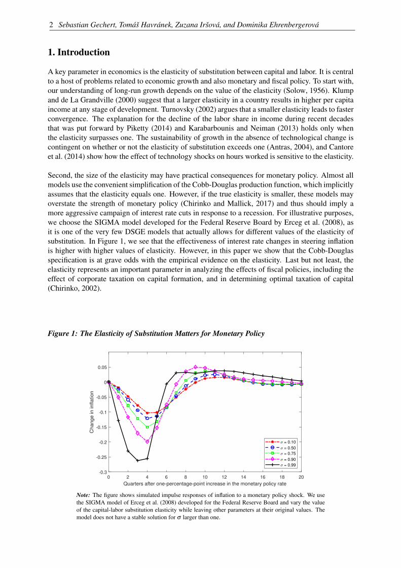
Second, the size of the elasticity may have practical consequences for monetary policy. Almost allmodels use the convenient simplification of the Cobb-Douglas production function, which implicitlyassumes that the elasticity equals one. However, if the true elasticity is smaller, these models mayoverstate the strength of monetary policy (Chirinko and Mallick, 2017) and thus should imply amore aggressive campaign of interest rate cuts in response to a recession. For illustrative purposes,we choose the SIGMA model developed for the Federal Reserve Board by Erceg et al. (2008), asit is one of the very few DSGE models that actually allows for different values of the elasticity ofsubstitution. In Figure 1, we see that the effectiveness of interest rate changes in steering inflationis higher with higher values of elasticity. However, in this paper we show that the Cobb-Douglasspecification is at grave odds with the empirical evidence on the elasticity. Last but not least, theelasticity represents an important parameter in analyzing the effects of fiscal policies, including theeffect of corporate taxation on capital formation, and in determining optimal taxation of capital(Chirinko, 2002).
Figure 1: The Elasticity of Substitution Matters for Monetary Policy
0 2 4 6 8 10 12 14 16 18 20
Quarters after one-percentage-point increase in the monetary policy rate
-0.3
-0.25
-0.2
-0.15
-0.1
-0.05
0
0.05
Ch
an
ge
in
in
fla
tio
n
= 0.10
= 0.50
= 0.75
= 0.90
= 0.99
Note: The figure shows simulated impulse responses of inflation to a monetary policy shock. We usethe SIGMA model of Erceg et al. (2008) developed for the Federal Reserve Board and vary the valueof the capital-labor substitution elasticity while leaving other parameters at their original values. Themodel does not have a stable solution for σ larger than one.

Death to the Cobb-Douglas Production Function? A Quantitative Survey of the Capital-LaborSubstitution Elasticity 3
Aside from convenience, the other reason for the widespread use of the Cobb-Douglas productionfunction is that, at first sight, empirical investigations into the value of the elasticity have producedmany central estimates close to 1. When each study gets the same weight, the mean elasticity re-ported in the literature reaches 0.9—at least based on our attempt to collect all published estimates,in total 3,186 coefficients from 121 studies. But we show that the picture is seriously distorted bypublication bias. After correcting for the bias, the mean reported elasticity shrinks to 0.5. More-over, some data and method choices affect the estimated elasticity systematically. If one agrees thatsector-level data dominate more aggregated country- or state-level data and that including infor-mation from the first-order condition for capital dominates ignoring it, the implied mean estimatefurther decreases to 0.3. We recommend this value for the calibration of the elasticity.
The finding of strong publication bias predominates in our results. The bias arises when differentestimates have a different probability of being reported depending on sign and statistical signifi-cance. The identification builds on the fact that almost all econometric techniques used to estimatethe elasticity assume that the ratio of the estimate to its standard error has a symmetrical distribution,typically a t-distribution. So the estimates and standard errors should represent independent quanti-ties. But if statistically significant positive estimates are preferentially selected for publication, largestandard errors (given by noise in data or imprecision in estimation) will become associated withlarge estimates. Because empirical economists command plenty of degrees of freedom, a large es-timate of the elasticity can always emerge if the researcher looks for it long enough, and an upwardbias in the literature arises. A useful analogy appears in McCloskey and Ziliak (2019), who likenpublication bias to the Lombard effect in biology: speakers increase their effort in the presenceof noise. Apart from linear techniques based on the Lombard effect, we employ recently devel-oped methods by Ioannidis et al. (2017), Andrews and Kasy (2019), Bom and Rachinger (2019),and Furukawa (2019), which account for the potential nonlinearity between the standard error andselection effort.
The studies in our dataset do not estimate a single population parameter; rather, the precise inter-pretation of the elasticity differs depending on the context in which authors derive their results.We collect 71 variables that reflect the different contexts and find that our conclusions regardingpublication bias hold when we control for context. Because of the richness of the literature on theelasticity of substitution, we face substantial model uncertainty with many controls and address it byusing Bayesian (Eicher et al., 2011; Steel, 2019) and frequentist (Hansen, 2007; Amini and Parme-ter, 2012) model averaging. We investigate how the estimated elasticities depend on publicationbias and the data and methods used in the analysis. Our results suggest that three factors drive theheterogeneity in the literature: publication bias (the size of the standard error), aggregation of in-put data (industry-level vs. country-level), and identification approach (whether or not informationfrom the first-order condition for capital is ignored). In addition, the normalization of the productionfunction used in recent studies typically brings much smaller reported elasticities, by 0.3 on average.We also find that different assumptions regarding technical change have little systematic effect onthe reported elasticity and that estimations using systems of equations tend to deliver results similarto those of single-equation approaches focused on the first-order condition for capital.
As the bottom line of our analysis, we construct a synthetic study that uses all the estimates reportedin the literature but assigns more weight to those that are arguably better specified. The result rep-resents a mean estimate implied by the literature but conditional on the absence of publication bias,use of best-practice methodology, and other aspects of quality (such as publication in a leadingjournal). In this way we obtain an elasticity of 0.3, the best guess we can make about the parameterunderpinned by half a century of accumulated empirical evidence. Defining best-practice method-ology, of course, is subjective, and different authors will have different preferences on the various
4 Sebastian Gechert, Tomáš Havránek, Zuzana Iršová, and Dominika Ehrenbergerová
aspects of study design. But to arrive at 0.3, it is enough to hold two preferences: (i) industry-leveldata are superior to more aggregated country-level data, and (ii) including information from thefirst-order condition for capital is superior to ignoring it. To put these numbers into perspective,we once again turn to the Fed’s SIGMA model, which employs a value of 0.5 for the elasticity ofsubstitution (Erceg et al., 2008). This calibration corresponds to the mean estimate in the literaturecorrected for publication bias, without discounting any estimates based on data and methodology.The model employed by the Bank of Finland (Kilponen et al., 2016), on the other hand, uses anelasticity of 0.85, which is close to the mean estimate in the literature without correcting for publi-cation bias. The calibration closest to our final result is that of Cantore et al. (2015), who use a priorof 0.4. Their posterior estimate is even lower, though, at below 0.2.
The remainder of the paper is structured as follows: section 2 briefly discusses how the elasticity ofsubstitution is estimated; section 3 describes how we collect estimates of the elasticity from primarystudies and provides a bird’s-eye view of the data; section 4 examines publication bias; section 5investigates the drivers of heterogeneity in the reported elasticities and calculates the mean elasticityimplied by best practice in the literature; and section 6 concludes the paper. Appendixes A and B de-scribe the bias-correction techniques designed by Furukawa (2019) and Andrews and Kasy (2019).Appendix C shows summary statistics of the variables that reflect study context, Appendix Dpresents robustness checks, and Appendix E includes the list of studies from which we extractestimates. The data and code are available in an online appendix at meta-analysis.cz/sigma.
2. Estimating the Elasticity
To set the stage for data collection and the identification of factors driving heterogeneity in re-sults, we provide a short description of the most common approaches to estimating the elasticityof substitution between capital and labor. The concept was introduced by Hicks (1932) and almostsimultaneously and independently by Robinson (1933), whose more popular definition treats theelasticity as the percentage change of the ratio of two production factors divided by the percentagechange of the ratio of their marginal products. Under perfect competition, both inputs are paid theirmarginal products, so the elasticity of substitution can be written as
σ =d(K/L)/(K/L)d(w/r)/(w/r)
=−d log(K/L)d log(r/w)
, (1)
where K and L denote capital and labor, r is the rental price of capital, and w is the wage rate. Undera quasiconcave production function, the elasticity attains any number in the interval (0,∞). If σ = 0,capital and labor are perfect complements, always used in a fixed proportion in the Leontief produc-tion function. If the elasticity lies in the interval (0,1), capital and labor form gross complements. Ifσ = 1, the production function becomes Cobb-Douglas, and the relative change in quantity becomesexactly proportional to the relative change in prices. If the elasticity lies in the interval (1,∞), capitaland labor form gross substitutes.
Although the concept of the elasticity of substitution was introduced in the 1930s, empirical esti-mates were only enabled by an innovation that came more than 20 years later: the introduction ofthe constant elasticity of substitution (CES) production function by Solow (1956), later popularizedby Arrow et al. (1961). The CES production function can be written as
Yt =C[π(AKt Kt)
σ−1σ +(1−π)(AL
t Lt)σ−1
σ ]σ
σ−1 , (2)
where σ denotes the elasticity of substitution, K and L are capital and labor, C is an efficiency pa-rameter, and π is a distributional parameter. The fraction σ−1
σis often labeled as ρ , a transformation
Death to the Cobb-Douglas Production Function? A Quantitative Survey of the Capital-LaborSubstitution Elasticity 5
of the elasticity called the substitution parameter. AKt and AL
t denote the level of efficiency of therespective inputs, and variations in AK
t and ALt over time reflect capital- and labor-augmenting tech-
nological change. When AKt = AL
t = At , technological change becomes Hicks-neutral, which meansthat the marginal rate of substitution does not change when an innovation occurs.
The CES production function is nonlinear in parameters, and in contrast to the Cobb-Douglas case, asimple analytical linearization does not emerge. Thus the CES production function can be estimated(i) in its nonlinear form, (ii) in a linearized form as suggested by Kmenta (1967), or (iii) by usingfirst-order conditions (FOCs). Kmenta (1967) introduced a logarithmized version of Equation 2with Hicks-neutral technological change:
logYt = logC+σ
σ −1log[
πKσ−1
σ
t +(1−π)Lσ−1
σ
t
](3)
and then applied a second-order Taylor series expansion to the term log[·] around the point σ = 1 toarrive at a function linear in σ :
logYt = logC+π logKt +(1−π) logLt −(σ −1)π(1−π)
2σ(logKt − logLt)
2. (4)
Estimation of σ via first-order conditions was first suggested by Arrow et al. (1961). The underlyingassumptions involve constant returns to scale and fully competitive factor and product markets. TheFOC with respect to capital can be written as follows:
log(
YtKt
)= σ log
(1π
)+(1−σ) log(AK
t C)+σ log(
rtpt
). (5)
Consequently, the FOC with respect to labor implies
log(
YtLt
)= σ log
(1
1−π
)+(1−σ) log(AL
t C)+σ log(
wtpt
), (6)
where p is the price of the output. The two conditions can be combined to yield
log(
KtLt
)= σ log
(π
1−π
)+(σ −1) log
(AK
tAL
t
)+σ log
(wtrt
). (7)
In a similar way, one can derive FOCs with respect to the labor share (wL)/Y , the capital share(rK)/Y , or their reversed counterparts. The FOCs can be estimated separately as single equations,within a system of two or three FOCs, and as a system of FOCs coupled with a nonlinear or lin-earized CES production function. The latter approach (also called the supply-side system approach)has become especially popular in recent studies. León-Ledesma et al. (2010) assert that usingthe supply-side system approach dominates one-equation estimation, especially when coupled withcross-equation restrictions and normalization, which was suggested by de La Grandville (1989) andKlump and de La Grandville (2000). After scaling technological progress so that AK
0 = AL0 = 1, the
normalized production function can be written as
Yt = Y0
π0
(AK
t KtK0
)σ−1σ
+(1−π0)
(AL
t LtL0
)σ−1σ
σ
σ−1
, (8)
6 Sebastian Gechert, Tomáš Havránek, Zuzana Iršová, and Dominika Ehrenbergerová
where π0 = r0K0/(r0K0 +w0L0) denotes the capital income share evaluated at the point of nor-malization. The point of normalization can be defined, for instance, in terms of sample means.In other words, normalization means rewriting the production function in indexed number form(Klump et al., 2012). Normalization makes it possible to overcome the “impossibility theorem” asdescribed in Diamond et al. (1978), i.e., to identify both the elasticity of substitution and the growthrates of biased technical change (León-Ledesma et al., 2010; Cantore and Levine, 2012), and haspartly led to a revival of the CES production function in empirical research (Klump et al., 2007,2008).1
Though the aforementioned approaches to estimating the elasticity dominate the literature, we alsoconsider other approaches, in particular the translog production function. The translog function isquadratic in the logarithms of inputs and outputs and provides a second-order approximation to anyproduction frontier (now omitting subscript t for ease of exposition):
logY = logα0 +∑i
αi logXi +12 ∑
i∑
jαi j logXi logX j, (9)
where α0 denotes the state of technological knowledge, and Xi and X j are inputs, in our case capitaland labor. The translog production frontier provides a wider set of options for substitution andtransformation patterns than a frontier based on the CES production function. Due to the dualityprinciple, researchers often employ the translog cost function instead:
logC = α0 + θ1 logY +12
θ2(logY )2 +∑i
βi logPi +12 ∑
i∑
jεi j logPi logPj +∑
iδi logPi logY, (10)
where C denotes total costs and i = K,L, and Pi is the input factor price (that is, w and r). UsingSheppard’s lemma, the following cost share functions can be derived:
Si = βi +∑i
εi j logPj +δi logY, (11)
where Si denotes the share of the i-th factor in total costs. In this case, Allen partial elasticities ofsubstitution are most often estimated and are defined as
σi j =γi j +SiS j
SiS j. (12)
We include estimates from all of the above-mentioned specifications, as each of them provides ameasure of the elasticity of substitution between capital and labor, broadly defined. Then we controlfor the various aspects of the context in which researchers obtain their estimates. These aspects arepresented and discussed in detail later in section 5, while the following section describes the datasetof the estimated elasticities.1 In fact, there is much more to normalization than representation in indexed number form, as shown in Cantoreand Levine (2012) and De La Grandville (2009). The parameters in a non-normalized production function do nothave economic interpretation (i.e., they are not deep): Cantore and Levine (2012) show that without normalization,only the elasticity of substitution is dimensionless; the other two key parameters—the efficiency and distributionparameters (see Eq. 2)—are dimensional, i.e., they depend on the elasticity of substitution and factor income sharesand thus can change with the choice of units of inputs and outputs. Cantore and Levine (2012) show that next tothe indexed number form representation, i.e., the form of deviation about a reference point, there is another optionfor creating dimensionless parameters, called re-parametrization. Nevertheless, most of the empirical literature wesurvey deals with normalization in the way shown in Eq. 8.
Death to the Cobb-Douglas Production Function? A Quantitative Survey of the Capital-LaborSubstitution Elasticity 7
3. Data
We use Google Scholar to search for studies estimating the elasticity. Google’s algorithm goesthrough the full text of studies, thus increasing the coverage of suitable published estimates, irre-spective of the precise formulation of the study’s title, abstract, and keywords. Our search query,available in the online appendix, is calibrated so that it yields the best-known relevant studies amongthe first hits. We examine the first 500 papers returned by the search. In addition, we inspect thelists of references in these studies and their Google Scholar citations to check whether we can findusable studies not captured by our baseline search—a method called “snowballing” in the literatureon research synthesis. We terminate the search on August 1, 2018, and do not add any new studiesbeyond that date.
To be included in our dataset, a study must satisfy three criteria. First, at least one estimate in thestudy must be directly comparable with the estimates described in section 2. Second, the study mustbe published. This criterion is mostly due to feasibility, since even after restricting our attentionto published studies the dataset involves the manual collection of hundreds of thousands of datapoints. Moreover, we expect published studies to exhibit higher quality on average and to containfewer typos and mistakes in reporting their results. Note that the inclusion of unpublished papers isunlikely to alleviate publication bias (Rusnak et al., 2013): researchers write their papers with theintention to publish.2 Third, the study must report standard errors or other statistics from which thestandard error can be computed. If the elasticity is not reported directly but can be derived from thepresented results, we use the delta method to approximate the standard error. Omitting the estimateswith approximated standard errors does not change our results up to a second decimal place.
Using the search algorithm and inclusion criteria described above, we collect 3,186 estimates ofthe elasticity of substitution from 121 studies. To our knowledge, this makes our paper the largestmeta-analysis conducted in economics so far: Doucouliagos and Stanley (2013), for example, sur-vey dozens of meta-analyses and find that the largest one uses 1,460 estimates. Ioannidis et al.(2017) report that the mean number of estimates used in economics meta-analyses is 400. The lit-erature on the elasticity of substitution is vast, with a long tradition spanning six decades and morethan 100 countries. The list of the studies we include in the dataset (we call them “primary studies”)is available in Appendix E. Out of the 121 studies, 39 are published in the five leading journals ineconomics. Altogether, they have received more than 20,000 citations in Google Scholar, highlight-ing the importance of the topic.
The mean reported estimate of the elasticity of substitution is 0.9 when we give the same weightto each study; that is, when we weight the estimates by the inverse of the number of observationsreported per study. The simple mean of all the estimates is 0.8. We consider the weighted mean to bemore informative, because the simple mean is driven by studies that report many estimates, typicallythe results of robustness checks, and we see little reason to place more weight on such studies. Forboth such constructed means, in any case, the deviation from the Cobb-Douglas specification is notdramatic, and one could use the mean estimate from the literature as a justification of why the Cobb-Douglas production function presents a solid approximation of the data. We will argue that such aninterpretation of the data misleads the reader because of publication bias and misspecifications inthe literature.
2 A more precise label for publication bias is therefore “selective reporting”, but we use the former, more commonone to maintain consistency with previous studies on the topic, such as DeLong and Lang (1992), Card and Krueger(1995), and Ashenfelter and Greenstone (2004).
8 Sebastian Gechert, Tomáš Havránek, Zuzana Iršová, and Dominika Ehrenbergerová
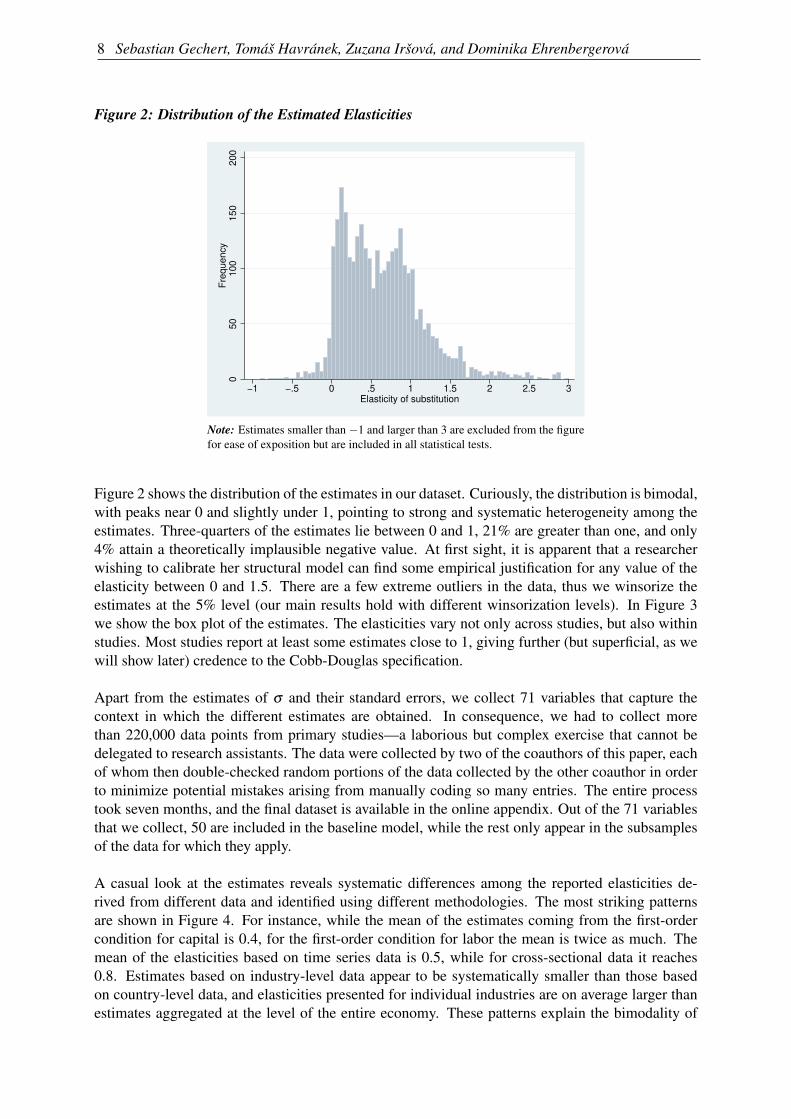
Figure 2: Distribution of the Estimated Elasticities
050
100
150
200
Fre
quency
−1 −.5 0 .5 1 1.5 2 2.5 3Elasticity of substitution
Note: Estimates smaller than −1 and larger than 3 are excluded from the figurefor ease of exposition but are included in all statistical tests.
Figure 2 shows the distribution of the estimates in our dataset. Curiously, the distribution is bimodal,with peaks near 0 and slightly under 1, pointing to strong and systematic heterogeneity among theestimates. Three-quarters of the estimates lie between 0 and 1, 21% are greater than one, and only4% attain a theoretically implausible negative value. At first sight, it is apparent that a researcherwishing to calibrate her structural model can find some empirical justification for any value of theelasticity between 0 and 1.5. There are a few extreme outliers in the data, thus we winsorize theestimates at the 5% level (our main results hold with different winsorization levels). In Figure 3we show the box plot of the estimates. The elasticities vary not only across studies, but also withinstudies. Most studies report at least some estimates close to 1, giving further (but superficial, as wewill show later) credence to the Cobb-Douglas specification.
Apart from the estimates of σ and their standard errors, we collect 71 variables that capture thecontext in which the different estimates are obtained. In consequence, we had to collect morethan 220,000 data points from primary studies—a laborious but complex exercise that cannot bedelegated to research assistants. The data were collected by two of the coauthors of this paper, eachof whom then double-checked random portions of the data collected by the other coauthor in orderto minimize potential mistakes arising from manually coding so many entries. The entire processtook seven months, and the final dataset is available in the online appendix. Out of the 71 variablesthat we collect, 50 are included in the baseline model, while the rest only appear in the subsamplesof the data for which they apply.
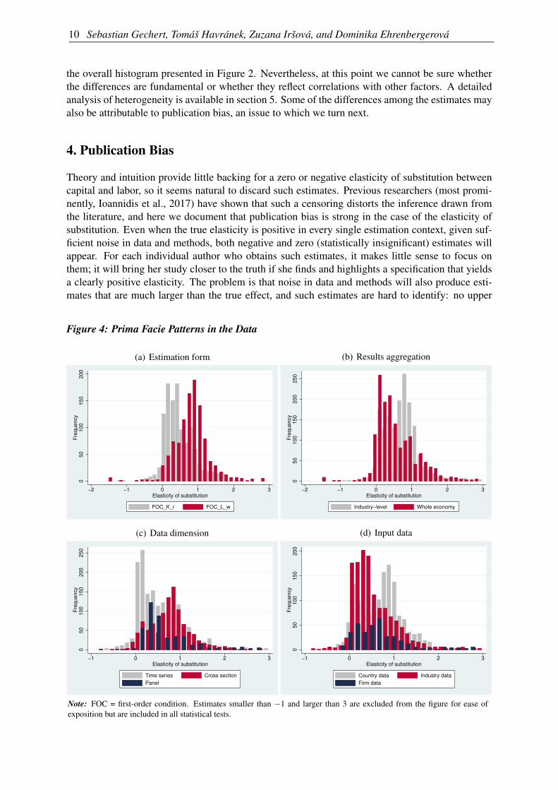
A casual look at the estimates reveals systematic differences among the reported elasticities de-rived from different data and identified using different methodologies. The most striking patternsare shown in Figure 4. For instance, while the mean of the estimates coming from the first-ordercondition for capital is 0.4, for the first-order condition for labor the mean is twice as much. Themean of the elasticities based on time series data is 0.5, while for cross-sectional data it reaches0.8. Estimates based on industry-level data appear to be systematically smaller than those basedon country-level data, and elasticities presented for individual industries are on average larger thanestimates aggregated at the level of the entire economy. These patterns explain the bimodality of

Death to the Cobb-Douglas Production Function? A Quantitative Survey of the Capital-LaborSubstitution Elasticity 9
Figure 3: Estimates Vary Both Across and Within Studies
−1 0 1 2 3Elasticity of substitution
van der Werf (2008)Zarembka (1970)
Young (2013)Williams and Laumas (1984)
Weitzman (1970)Tsang and Persky (1975)Tevlin and Whelan (2003)
Solow (1964)Smith (2008)
Semieniuk (2017)Schmitz (1981)Schaller (2006)
Saxonhouse (1977)Sato and Hoffman (1968)
Sato (1977)Sapir (1980)
Sankar (1972)Salvanes (1989)
Sahota (1966)Roskamp (1977)
Raurich et al. (2012)Pollak et al. (1984)
Parks (1971)Panik (1976)Nadiri (1968)
Moroney and Toevs (1977)Moroney and Allen (1969)
Moroney (1970)Moroney (1966)
Mohabbat et al. (1984)Mohabbat and Dalal (1983)
Minasian (1961)Meller (1975)
McLean−Meyinsse and Okunade (1988)McKinnon (1962)McCallum (1985)
McAdam and Willman (2004)Masanjala and Papageorgiou (2004)
Martin et al. (1993)Mallick (2012)
Luoma and Luoto (2010)Lovell (1973b)Lovell (1973a)
Lin and Shao (2006)Lianos (1975)Lianos (1971)
Leung and Yuen (2010)Leon−Ledesma et al. (2015)
Lee and Tcha (2004)Krusell (2000)
Kmenta (1967)Klump et al. (2008)Klump et al. (2007)
Kislev and Peterson (1982)Kilponen and Viren (2010)
Karabarbounis and Neiman (2014)Kalt (1978)
Judzik and Sala (2015)Jones and Backus (1977)
Jalava et al. (2006)Iqbal (1986)
Humphrey and Moroney (1975)Hossain (1987)
Hijzen and Swaim (2010)Herrendorf et al. (2015)
Griliches (1967)Griliches (1964)
Fuchs (1963)Fitchett (1976)
Fishelson (1979)Ferguson (1965)
Felipe and McCombie (2009)Feldstein and Flemming (1971)
Feldstein (1967)Emran et al. (2007)
Ellis and Price(2004)Elbers et al. (2007)
Eisner and Nadiri (1968)Eisner (1969)Eisner (1967)
Easterly and Fischer (1995)Dwenger (2014)
Duffy and Papageorgiou (2000)Donges (1972)
Dissou et al. (2015)Dissou and Ghazal (2010)
Dhrymes (1965)David and van de Klundert (1965)
Daniels (1969)Cummins et al. (1994)
Cummins and Hasset (1992)Claro (2003)Clark (1993)
Chwelos et al. (2010)Chirinko et al. (2011)Chirinko et al. (1999)
Chirinko and Mallick (2017)Chetty and Sankar (1969)
Caballero (1994)Bruno and Sachs (1982)
Brox and Fader (2005)Brown and de Cani (1963a)
Brown (1966)Bodkin and Klein (1967)
Blanchard (1977)Binswanger (1974)
Berthold et al. (2002)Berndt (1976)
Bentolila and Saint−Paul (2003)Behrman (1982)Behrman (1972)
Bartelsman and Beetsma (2003)Balistreri et al. (2003)
Asher (1972)Artus (1984)
Arrow et al. (1961)Apostolakis (1984)
Antras (2004)Akay and Dogan (2013)
Abed (1975)
Note: The figure shows a box plot of the estimates of the elasticity of substitution reported in individual studies. The boxshows the interquartile range (P25–P75) and the median highlighted. Whiskers cover (P25 − 1.5*interquartile range) to (P75+ 1.5*interquartile range). The dots are remaining (outlying) estimates. Estimates smaller than −1 and larger than 3 areexcluded from the figure for ease of exposition but are included in all statistical tests.
10 Sebastian Gechert, Tomáš Havránek, Zuzana Iršová, and Dominika Ehrenbergerová
the overall histogram presented in Figure 2. Nevertheless, at this point we cannot be sure whetherthe differences are fundamental or whether they reflect correlations with other factors. A detailedanalysis of heterogeneity is available in section 5. Some of the differences among the estimates mayalso be attributable to publication bias, an issue to which we turn next.
4. Publication Bias
Theory and intuition provide little backing for a zero or negative elasticity of substitution betweencapital and labor, so it seems natural to discard such estimates. Previous researchers (most promi-nently, Ioannidis et al., 2017) have shown that such a censoring distorts the inference drawn fromthe literature, and here we document that publication bias is strong in the case of the elasticity ofsubstitution. Even when the true elasticity is positive in every single estimation context, given suf-ficient noise in data and methods, both negative and zero (statistically insignificant) estimates willappear. For each individual author who obtains such estimates, it makes little sense to focus onthem; it will bring her study closer to the truth if she finds and highlights a specification that yieldsa clearly positive elasticity. The problem is that noise in data and methods will also produce esti-mates that are much larger than the true effect, and such estimates are hard to identify: no upper
Figure 4: Prima Facie Patterns in the Data
(a) Estimation form
05
01
00
15
02
00
Fre
qu
en
cy
−2 −1 0 1 2 3Elasticity of substitution
FOC_K_r FOC_L_w
(b) Results aggregation
05
01
00
15
02
00
25
0F
req
ue
ncy
−2 −1 0 1 2 3Elasticity of substitution
Industry−level Whole economy
(c) Data dimension
05
01
00
15
02
00
25
0F
req
ue
ncy
−1 0 1 2 3Elasticity of substitution
Time series Cross section
Panel
(d) Input data
05
01
00
15
02
00
Fre
qu
en
cy
−1 0 1 2 3Elasticity of substitution
Country data Industry data
Firm data
Note: FOC = first-order condition. Estimates smaller than −1 and larger than 3 are excluded from the figure for ease ofexposition but are included in all statistical tests.
Death to the Cobb-Douglas Production Function? A Quantitative Survey of the Capital-LaborSubstitution Elasticity 11
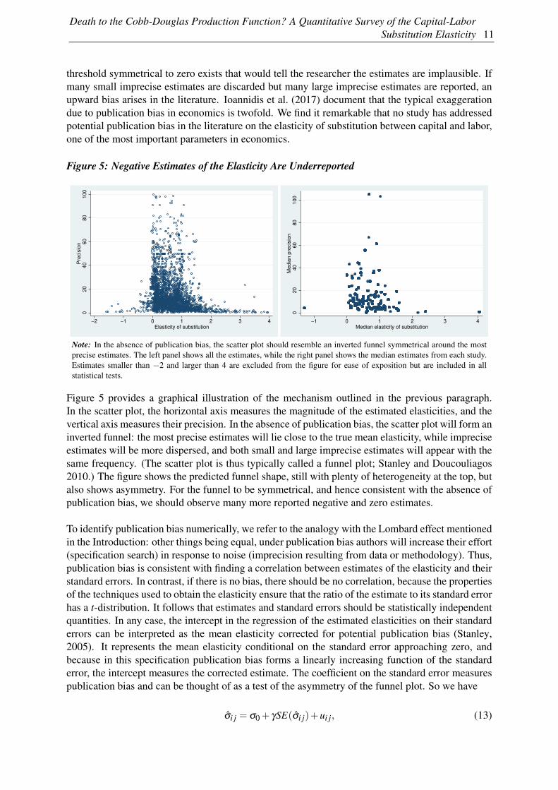
threshold symmetrical to zero exists that would tell the researcher the estimates are implausible. Ifmany small imprecise estimates are discarded but many large imprecise estimates are reported, anupward bias arises in the literature. Ioannidis et al. (2017) document that the typical exaggerationdue to publication bias in economics is twofold. We find it remarkable that no study has addressedpotential publication bias in the literature on the elasticity of substitution between capital and labor,one of the most important parameters in economics.
Figure 5: Negative Estimates of the Elasticity Are Underreported
02
04
06
08
01
00
Pre
cis
ion
−2 −1 0 1 2 3 4Elasticity of substitution
02
04
06
08
01
00
Me
dia
n p
recis
ion
−1 0 1 2 3 4Median elasticity of substitution
Note: In the absence of publication bias, the scatter plot should resemble an inverted funnel symmetrical around the mostprecise estimates. The left panel shows all the estimates, while the right panel shows the median estimates from each study.Estimates smaller than −2 and larger than 4 are excluded from the figure for ease of exposition but are included in allstatistical tests.
Figure 5 provides a graphical illustration of the mechanism outlined in the previous paragraph.In the scatter plot, the horizontal axis measures the magnitude of the estimated elasticities, and thevertical axis measures their precision. In the absence of publication bias, the scatter plot will form aninverted funnel: the most precise estimates will lie close to the true mean elasticity, while impreciseestimates will be more dispersed, and both small and large imprecise estimates will appear with thesame frequency. (The scatter plot is thus typically called a funnel plot; Stanley and Doucouliagos2010.) The figure shows the predicted funnel shape, still with plenty of heterogeneity at the top, butalso shows asymmetry. For the funnel to be symmetrical, and hence consistent with the absence ofpublication bias, we should observe many more reported negative and zero estimates.
To identify publication bias numerically, we refer to the analogy with the Lombard effect mentionedin the Introduction: other things being equal, under publication bias authors will increase their effort(specification search) in response to noise (imprecision resulting from data or methodology). Thus,publication bias is consistent with finding a correlation between estimates of the elasticity and theirstandard errors. In contrast, if there is no bias, there should be no correlation, because the propertiesof the techniques used to obtain the elasticity ensure that the ratio of the estimate to its standard errorhas a t-distribution. It follows that estimates and standard errors should be statistically independentquantities. In any case, the intercept in the regression of the estimated elasticities on their standarderrors can be interpreted as the mean elasticity corrected for potential publication bias (Stanley,2005). It represents the mean elasticity conditional on the standard error approaching zero, andbecause in this specification publication bias forms a linearly increasing function of the standarderror, the intercept measures the corrected estimate. The coefficient on the standard error measurespublication bias and can be thought of as a test of the asymmetry of the funnel plot. So we have
σi j = σ0 + γSE(σi j)+ui j, (13)

12 Sebastian Gechert, Tomáš Havránek, Zuzana Iršová, and Dominika Ehrenbergerová
where σ is the i-th estimated elasticity in study j, γ denotes the intensity of publication bias, and σ0represents the mean elasticity corrected for the bias.
In Table 1 we report the results of several specifications based on Equation 13. We cluster standarderrors at both the study and the country level, as estimates are unlikely to be independent withinthese two dimensions; our implementation of two-way clustering follows Cameron et al. (2011).We also report wild bootstrap confidence intervals (Cameron et al., 2008). In all specifications, wefind a statistically significant and positive coefficient on the standard error (publication bias) and asignificant and positive intercept (the mean elasticity corrected for the bias). After correcting forpublication bias, the mean elasticity drops from 0.9 to 0.5. The result is robust across all spec-ifications with the exception of one, which suggests an even stronger bias and smaller correctedelasticity.
Table 1: Linear Tests of Funnel Asymmetry Suggest Publication Bias
OLS FE BE Precision Study IV
SE (publication 0.881∗∗∗ 0.656∗∗∗ 1.111∗∗∗ 1.025∗∗∗ 0.888∗∗∗ 2.186∗∗∗
bias) (0.086) (0.201) (0.190) (0.115) (0.094) (0.413)[0.49; 1.21] − − [0.59; 1.40] [0.62; 1.22] [1.20; 3.68]
Constant (mean 0.492∗∗∗ 0.529∗∗∗ 0.499∗∗∗ 0.468∗∗∗ 0.544∗∗∗ 0.279∗∗∗
beyond bias) (0.028) (0.033) (0.048) (0.025) (0.039) (0.070)[0.38; 0.61] − − [0.36; 0.61] [0.44; 0.64] [0.04; 0.47]
Studies 121 121 121 121 121 121Observations 3,186 3,186 3,186 3,186 3,186 3,186
Note: The table presents the results of regression σi j = σ0 + γSE(σi j) + ui j. σi j and SE(σi j) are the i-th estimates ofthe elasticity of substitution and their standard errors reported in the j-th study. The standard errors of the regressionparameters are clustered at both the study and country level and shown in parentheses (the implementation of two-wayclustering follows Cameron et al., 2011). OLS = ordinary least squares. FE = study-level fixed effects. BE = study-levelbetween effects. Precision = the inverse of the reported estimate’s standard error is used as the weight. Study = the inverseof the number of estimates reported per study is used as the weight. IV = the inverse of the square root of the numberof observations employed by researchers is used as an instrument for the standard error. ∗∗∗, ∗∗, and ∗ denote statisticalsignificance at the 1%, 5%, and 10% level. Standard errors in parentheses. Whenever possible, in square brackets we alsoreport 95% confidence intervals from wild bootstrap clustering; the implementation follows Roodman (2019), and we useRademacher weights with 9,999 replications.
The first column of Table 1 reports a simple OLS regression. The second column adds study-levelfixed effects in order to account for unobserved study-specific characteristics, but little changes.(Adding country dummies would also produce similar results.) The third column uses between-study variance instead of within-study variance, and the estimate of the corrected mean remains notmuch affected. Next, we apply two weighting schemes. First, the precision becomes the weight,as suggested by Stanley and Doucouliagos (2017), which adjusts for the heteroskedasticity in theregression. Similar weights are used in physics for meta-analyses of particle mass estimates (Bakerand Jackson, 2013). The corrected mean elasticity becomes a bit smaller, but is not far from 0.5.Second, we weight the data by the inverse of the number of observations reported in a study, so thateach study has the same impact on the results. Again, the difference is small in comparison to otherspecifications. In the last column, we report the results of an instrumental variable (IV) regression.IV represents a crucial robustness check, because in primary studies, estimates and standard errorsare jointly determined by the estimation technique. If some techniques produce systematically largerstandard errors and point estimates, our finding of publication bias could be spurious. An intuitiveinstrument for the standard error is the inverse of the square root of the number of observations used

Death to the Cobb-Douglas Production Function? A Quantitative Survey of the Capital-LaborSubstitution Elasticity 13
Table 2: Nonlinear Techniques Corroborate Publication Bias
Bom & Rachinger(2019)
Furukawa(2019)
Andrews& Kasy (2019)
Ioaninidiset al. (2017)
Mean beyond bias 0.52 0.55 0.43 0.50(0.09) (0.21) (0.02) (0.06)
Note: Standard errors in parentheses. The method developed by Bom and Rachinger (2019) searches for a precisionthreshold above which publication bias is unlikely. The methods developed by Furukawa (2019) and Andrews and Kasy(2019) are described in detail in Appendixes A and B. The method developed by Ioannidis et al. (2017) focuses on estimateswith adequate power.
in the primary study: the root is correlated with the standard error by definition but is unlikely tobe very correlated with the use of a particular estimation technique. Using IV we obtain a largerestimate of publication bias and a smaller estimate of the mean elasticity corrected for publicationbias, 0.3.3
The simple tests based on the Lombard effect and presented in Table 1 are intuitive but can them-selves be biased if publication selection does not form a linear function of the standard error. Forexample, it might be the case that estimates are automatically reported if they cross a particularprecision threshold. This is the intuition behind the estimator due to Bom and Rachinger (2019)presented in Table 2. Bom and Rachinger (2019) show how to estimate this threshold for eachliterature and introduce an “endogenous kink” technique that extends the linear test based on theLombard effect. Next, Furukawa (2019) provides a nonparametric method that is robust to vari-ous assumptions regarding the functional form of publication bias and the underlying distributionof true effects. Furukawa (2019) suggests using only a portion of the most precise estimates, thestem of the funnel plot, and determines this portion by minimizing the trade-off between variance(decreasing in the number of estimates included) and bias (increasing in the number of impreciseestimates included). The stem-based method is generally more conservative than those commonlyused, producing wide confidence intervals; the details are available in Appendix A.
Another nonlinear method to correct for publication bias is advocated by Andrews and Kasy (2019).They show how the conditional publication probability (the probability of publication as a functionof a study’s results) can be nonparametrically identified and then describe how publication biascan be corrected for if the conditional publication probability is known. The underlying intuitioninvolves jumps in publication probability at conventional p-value cut-offs. Using their method, weestimate that positive elasticities are six times more likely to be published than negative ones. Weinclude more details on the approach and estimation in Appendix B. Finally, the remaining estimatein Table 2 arises using the approach championed by Ioannidis et al. (2017), who focus only onestimates with adequate statistical power. We conclude that both linear and nonlinear techniquesagree that 0.5 represents a robust estimate of the mean elasticity of substitution after correctingthe literature for publication bias. Since the uncorrected mean equals 0.9, the exaggeration due topublication bias is almost twofold, consistent with the rule of thumb suggested by Ioannidis et al.(2017). Therefore, when we give the same weight to all approaches used in primary studies, theempirical literature as a whole provides no support for the Cobb-Douglas production function. Butperhaps poor data and misspecifications bias the mean estimate downwards. We investigate thisissue in the next section.3 The result is consistent with some estimation techniques or aspects of data influencing the point estimates andstandard errors in opposite directions. In the next section we explicitly control for 71 aspects of study design,including data and methodology, and our final estimate also equals 0.3.

14 Sebastian Gechert, Tomáš Havránek, Zuzana Iršová, and Dominika Ehrenbergerová
5. Heterogeneity
In section 2 and section 3 we discussed several prominent aspects of study design that might system-atically influence the reported estimates of the elasticity. But many additional study characteristicscan certainly play a role, and we need to control for them. To assign a pattern to the apparent hetero-geneity in the literature, we collect 71 variables that reflect the context in which researchers obtaintheir estimates. The variables capture the characteristics of the data, specification choice, econo-metric approach, definition of the production function, and publication characteristics. (Moreover,the effects of different ways of measuring capital and labor are examined in subsamples of the maindataset and presented in Appendix D.) The variables, grouped in these categories, are discussed be-low and listed in Table C1 and Table C2 in Appendix C together with their definitions and summarystatistics.
5.1 Variables
Data characteristics A central distinguishing feature of the studies concerns the level of data ag-gregation. Almost half (45%) of the studies employ country- or state-level data, which forms ourreference category. We include a dummy variable equal to one if the study uses industry-leveldata (43% of the estimates) and firm-level data (12% of the estimates). We also include a dummyequal to one when the resulting estimate does not represent the whole economy but is reported ata disaggregated level for various industries. Moreover, we add controls for potential cross-countrydifferences: a dummy for the US, developed European countries, and developing countries, as thesubstitutability between capital and labor may differ with the level of economic development andacross institutional settings. For instance, Duffy and Papageorgiou (2000) suggest that capital andlabor become less substitutable in poorer countries.
To account for potential small-sample bias, we control for the number of observations used in eachstudy. We also include the midpoint of the data period to capture a potential positive trend in theelasticity over time, which could be due to economic development within a country, a changingcomposition of the inputs, or changes in their relative efficiency (Cantore et al., 2017). Regardingdata frequency, 89% of the estimates employ annual data; we thus use annual data as the baselinecategory and include a dummy variable for the use of quarterly data. Moreover, we control fordata dimension—whether time series, cross-sectional, or panel data are used. Most of the studies(around 53%) employ time series data, which we take as the reference category.
The final subset of variables covering data characteristics describes the source of data. Many es-timates are based on data from the same databases—the largest number of studies employ datafrom the US Annual Survey of Manufacturers and Census of Manufacturers. The second largestgroup is the KLEM database by Jorgenson (2007), followed by the OECD’s International SectoralDatabase and Structural Analysis Database. We do not have a prior on how data sources shouldaffect estimates, yet we still prefer not to ignore this potential source of variation and include thecorresponding dummies as control variables.
Specification Concerning the specification of the various studies described in section 2, we distin-guish between estimation via single first-order conditions (FOCs), systems of more than one FOC,systems of the production function plus FOCs, linear approximations of the production function,and nonlinear estimation of the production function. We also discriminate between the FOC forlabor based on the wage rate, the FOC for capital based on the rental rate of capital, the FOC forthe capital-labor ratio based on the ratio between the wage rate and the rental rate of capital, the

Death to the Cobb-Douglas Production Function? A Quantitative Survey of the Capital-LaborSubstitution Elasticity 15
FOC for capital share, and the FOC for labor share in income. In total, this gives us nine distinctcategories for estimation specification. We choose the FOC for capital based on the rental rate asthe reference category because it represents the most frequently used specification (35%), thoughclosely followed by the FOC for labor based on the wage rate (33% of the estimates). A special caseof the FOC for capital is its inverse estimation, in which the resulting estimates are labeled user-costelasticities; examples include Smith (2008) and Chirinko et al. (2011).
Figure 6: Estimation Form Matters for the Reported Elasticities0
.51
1.5
Kern
el density
−1 0 1 2 3Elasticity of substitution
System PF+FOC System FOCs
Nonlinear Linear approximation
FOC_K_r FOC_L_w
FOC_KL_rw FOC_K_share
FOC_L_share
Note: A detailed description of the variables is available in Table C1.
The differences in the estimates derived from the various specifications are clearly visible in thedata (Figure 6). While the mean of the estimates derived from the FOC for labor based on the wagerate reaches 1.1, estimates derived from the FOC for capital based on the rental rate of capital are onaverage only 0.5. Estimates obtained from the linear approximation of the production function alsostand out, reaching a mean value of 1.1. Some of these patterns were noted early in the history ofthe estimation of the elasticity, for example by Berndt (1976), and later discussed by Antras (2004)and Young (2013). We attempt to quantify the patterns, while simultaneously controlling for otherinfluences.
Regarding system estimations, two other important specification aspects can influence the re-ported elasticities: normalization and cross-equation restrictions. Normalization, suggested byde La Grandville (1989), further explored by Klump and de La Grandville (2000), and first imple-mented empirically by Klump et al. (2007), has been used by only a small fraction of the studiesin our database. Normalization starts from the observation that a family of CES functions whosemembers are distinguished only by different elasticities of substitution needs a common bench-mark point. Since the elasticity of substitution is defined as a point elasticity, one needs to fixbenchmark values for the level of production, factor inputs, and the marginal rate of substitution, orequivalently for per capita production, capital deepening, and factor income shares. Normalizationimplies representing the production function in a consistent indexed number form (Klump et al.,2012). A proper choice of the point of normalization facilitates the identification of deep technicalparameters; in other words, it overcomes the “impossibility theorem” by enabling the elasticity ofsubstitution and growth rates of technical change to be identified at the same time (León-Ledesmaet al., 2010). According to León-Ledesma et al. (2010), the superiority of system estimation com-

16 Sebastian Gechert, Tomáš Havránek, Zuzana Iršová, and Dominika Ehrenbergerová
pared to the single FOC approach is further enhanced when complemented with normalization. Intheir Monte Carlo experiment, they show that without normalization, estimates tend towards one.
Some estimations of systems employ cross-equation restrictions that restrict parameters across twoor more equations to be equal, as in Zarembka (1970), Krusell et al. (2000), and Klump et al.(2007). To account for possible differences, we additionally include a dummy for cross-equationrestrictions.
While the vast majority of estimates come from single-level production functions, estimates of theelasticity of substitution between capital and labor can also be found in studies using two-level pro-duction functions, including additional inputs such as energy and material (e.g., Van der Werf, 2008;Dissou et al., 2015). We control for two-level production functions as a special case. Moreover,when estimates of the elasticity rely on such two-level production functions, linear approximationsof the production function, or a system of linear approximation in conjunction with share factors,researchers commonly report partial elasticities of substitution, for which we control as well. Ourresults are robust to excluding partial elasticities.
Econometric approach Our reference category for the choice of econometric technique is OLS.We include a dummy for the case when the model is dynamic, which holds for approximatelyone-quarter of all observations. The second dummy we include equals one if seemingly unrelatedregression (SUR) is used—it is often employed for the estimation of systems of equations (11% ofall estimates). An important aspect of estimating the elasticity, as pointed out by Chirinko (2008), iswhether the estimate refers to a long-run or a short-run elasticity. Our reference category consists ofexplicit long-run specifications, that is, models in which coefficients are meant to be long-run andthe specification is adjusted accordingly. We opt for long-run elasticities as a reference point as theyare regarded as more informative for economic decisions. Explicit long-run specifications includeestimations of cointegration relations or interval-difference models, where data are averaged overlonger intervals to mimic lower frequencies; distributed lag models can also give a long-run esti-mate. Conversely, the short-run approach modifies the estimating equation to account for temporaldynamics. Examples include estimation of implicit investment equations, as in Eisner and Nadiri(1968) or Eisner (1969), differenced models, and estimation of short-run elements from error cor-rection models or distributed lag models. The vast majority of estimates (70%) are meant to belong-run but the specification is unadjusted.
Production function components The fourth category of control variables comprises the ingre-dients of the production function. We include a dummy variable for the case when other inputs(energy, materials, human capital) are considered as additional factors of production, for instanceby Humphrey and Moroney (1975), Bruno and Sachs (1982), and Chirinko and Mallick (2017). Weinclude a dummy that equals one when a study differentiates between skilled and unskilled labor.We also subject the estimates to the following questions. Does the production function assumeHicks-neutral technological change (our reference category), Harrod-neutral technological change(i.e., labor-augmenting, LATC), or Solow-neutral technological change (i.e., capital-augmenting,CATC)? Are the dynamics of technological change important in explaining the heterogeneity? Thegrowth rate of technological change can be either zero (our reference), constant or—with flexibleBox and Cox (1964) transformation—exponential, hyperbolic, or logarithmic. According to the im-possibility theorem suggested by Diamond et al. (1978), it is infeasible to identify both the elasticityof substitution and the parameters of technological change at the same time, so researchers tend toimpose one of the three specific forms of technological change and implicit or explicit assumptionson its growth rate. We include the corresponding dummy variables.
Death to the Cobb-Douglas Production Function? A Quantitative Survey of the Capital-LaborSubstitution Elasticity 17
We distinguish between estimates of gross and net elasticity, based on whether gross or net data foroutput and the capital stock are used. As pointed out in Semieniuk (2017), the distinction betweennet and gross elasticity is important with respect to the inequality argument of Piketty (2014): for hisexplanation of the decline in the labor share to hold, σ needs to exceed one in net terms. Elasticitiesbased on net quantities should naturally yield smaller results (Rognlie, 2014). Finally, we includetwo additional dummies—first, for the case when researchers abandon the assumption of constantreturns to scale; second, for the case when researchers relax the assumption of perfectly competitivemarkets.
Publication characteristics We include four study-level variables: the year of the appearance ofthe first draft of the paper in Google Scholar, a dummy for the paper being published in a top fivejournal, the recursive discounted RePEc impact factor of the outlet, and the number of citations peryear since the first appearance of the paper in Google Scholar. We include these variables in orderto capture aspects of study quality not reflected by observable differences in data and methods.
Moreover, we include two additional dummies. The first variable measures whether the study’scentral focus is the elasticity of substitution between capital and labor or whether the estimate is abyproduct of a different exercise, such as in Cummins and Hassett (1992) and Chwelos et al. (2010).The second variable equals one if the author explicitly prefers the estimate in question, and equalsminus one if the estimate is explicitly discounted. Nevertheless, researchers typically do not revealtheir exact preferences regarding the individual estimates they produce, so the variable equals zerofor most estimates.
5.2 Estimation
An obvious thing to do at this point is to regress the reported elasticities on the variables reflectingthe context in which researchers obtain their estimates:
σi j = α0 +49
∑l=1
βlXl,i j + γSE(σi j)+µi j, (14)
where σi j again denotes estimate i of the elasticity of substitution reported in study j, Xl,i j representsthe control variables described in subsection 5.1, γ again denotes the intensity of publication bias,and α0 represents the mean elasticity corrected for publication bias but conditional on the definitionof the variables included in X—that is, the intercept means nothing on its own, and µi j stands forthe error term.
But using one regression is inadequate because of model uncertainty. With so many variables reflect-ing study design, including all of them would substantially attenuate the precision of our estimation.(We use 50 variables in the baseline estimation; the remaining 21 variables related to measurementof capital and labor and industry-level characteristics are included in the three subsamples presentedin Appendix D.) One solution is to reduce the number of variables to about 10, which could allowfor simple estimation—but doing so would ignore many aspects in which estimates and studies dif-fer. Another commonly applied solution to model uncertainty is stepwise regression, but sequentialt-tests are statistically problematic as individual variables can be excluded by accident. The solutionthat we choose here is Bayesian model averaging (BMA; see, for example, Eicher et al., 2011; Steel,2019), which arises naturally as a response to model uncertainty in the Bayesian setting.
BMA runs many regression models with different subsets of variables; in our case there are 250
possible subsets. Assigned to each model is a posterior model probability (PMP), an analog to
18 Sebastian Gechert, Tomáš Havránek, Zuzana Iršová, and Dominika Ehrenbergerová
information criteria in frequentist econometrics, measuring how well the model performs comparedto other models. The resulting statistics are based on a weighted average of the results from all theregressions, the weights being the posterior model probabilities. For each variable we thus obtaina posterior inclusion probability (PIP), which denotes the sum of the posterior model probabilitiesof all the models in which the variable is included. Using the laptop on which we wrote this paper,it would take us decades to estimate all the possible models, so we opt for a model compositionMarkov Chain Monte Carlo algorithm (Madigan and York, 1995) that walks through the modelswith the highest posterior model probabilities. In the baseline specification we use a uniform modelprior (each model has the same prior probability) and unit information g-prior (the prior that allregression coefficients equal zero has the same weight as one observation in the data), but we alsouse alternative priors in Appendix D.
Second, as a simple robustness check of our baseline BMA specification, we run a hybridfrequentist-Bayesian model. We employ variable selection based on BMA (specifically, we onlyinclude the variables with PIPs above 80%) and estimate the resulting model using OLS withclustered standard errors. We label this specification a “frequentist check” of the baseline BMAexercise. Third, we employ frequentist model averaging (FMA). Our implementation of FMAuses Mallows’s criteria as weights, since they prove asymptotically optimal (Hansen, 2007). Theproblem is that, using a frequentist approach, we have no straightforward alternative to the modelcomposition Markov Chain Monte Carlo algorithm, and it appears infeasible to estimate all 250
potential models. We therefore follow the approach suggested by Amini and Parmeter (2012) andresort to orthogonalization of the covariate space.
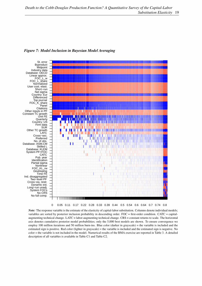
5.3 Results
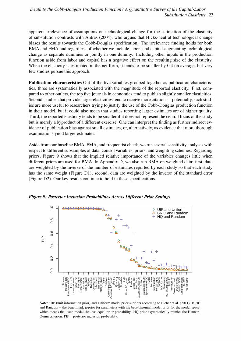
Figure 7 illustrates our results. The vertical axis depicts explanatory variables sorted by their poste-rior inclusion probabilities; the horizontal axis shows individual regression models sorted by theirposterior model probabilities. The blue color indicates that the corresponding variable appears inthe model and the estimated parameter has a positive sign, while the red color indicates that theestimated parameter is negative. In total, 21 variables appear to drive the heterogeneity in the esti-mates, as their posterior inclusion probabilities surpass 80%. Table 3 provides numerical results forBMA and the frequentist check. In the frequentist check we only include the 21 variables with PIPsabove 80%. Choosing a 50% threshold, for example, would result in including merely two morevariables with virtually unchanged results for the remaining ones. Figure 8 plots posterior coeffi-cient distributions of selected variables. The results of the FMA exercise are reported in Table D1in Appendix D.
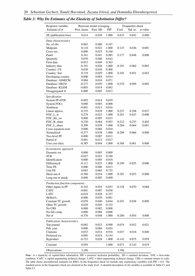
The first conclusion that we make based on these results is that our findings of publication bias pre-sented in the previous section remain robust when we control for the context in which the elasticityis estimated. Indeed, the variable corresponding to publication bias, the standard error of the esti-mate, represents the single most effective variable in explaining the heterogeneity in the reportedestimates of the elasticities of substitution (though several other variables also have posterior inclu-sion probabilities very close to 100% and are rounded to that number in Table 3). We observe thatthe publication bias detected by the correlation between estimates and standard errors is not drivenby aspects of data and methods omitted from the univariate regression in Equation 13.
Data characteristics Several characteristics related to the data used in primary studies systemati-cally affect the estimates of the elasticity. Our results suggest a mild upward trend in the reportedelasticities, which increase on average by 0.004 each year. (The yearly change does not equal the
Death to the Cobb-Douglas Production Function? A Quantitative Survey of the Capital-LaborSubstitution Elasticity 19
Figure 7: Model Inclusion in Bayesian Model Averaging
0 0.05 0.11 0.17 0.22 0.28 0.33 0.39 0.44 0.5 0.54 0.6 0.64 0.7 0.74 0.8
St. error Byproduct
MidpointIndustry data
Database: OECD Linear approx.
FOC_L_wFOC_L_share
NormalizedUser cost. elast.
Short−runNet sigma
Country: Eur DifferencedTop journal
FOC_K_share Panel
CitationsOther inputs in PF
Constant TC growth Unit FE
QuarterlyCountry: US
Firm data SUR
Other TC growth LATC
Cross−sec. Preferred
No. of obs. Database: ASM,CM
Skilled L Database: KLEM System PF+FOC
CATCPub. year
Identification Partial sigma
NonlinearFOC_KL_rw Developing
Time FEInd. disaggregated
Two−level PF Cross−eq. restr.
Dynamic est. Long−run unadj.
System FOCsNo CRS
No full comp.
Note: The response variable is the estimate of the elasticity of capital-labor substitution. Columns denote individual models;variables are sorted by posterior inclusion probability in descending order. FOC = first-order condition. CATC = capital-augmenting technical change. LATC = labor-augmenting technical change. CRS = constant returns to scale. The horizontalaxis denotes cumulative posterior model probabilities; only the 5,000 best models are shown. To ensure convergence weemploy 100 million iterations and 50 million burn-ins. Blue color (darker in grayscale) = the variable is included and theestimated sign is positive. Red color (lighter in grayscale) = the variable is included and the estimated sign is negative. Nocolor = the variable is not included in the model. Numerical results of the BMA exercise are reported in Table 3. A detaileddescription of all variables is available in Table C1 and Table C2.
20 Sebastian Gechert, Tomáš Havránek, Zuzana Iršová, and Dominika Ehrenbergerová
Table 3: Why Do Estimates of the Elasticity of Substitution Differ?
Response variable: Bayesian model averaging Frequentist checkEstimate of σ Post. mean Post. SD PIP Coef. Std. er. p-value
SE (publication bias) 0.614 0.038 1.000 0.633 0.042 0.000
Data characteristicsNo. of obs. 0.003 0.009 0.107Midpoint 0.118 0.022 1.000 0.123 0.036 0.001Cross-sec. 0.009 0.023 0.160Panel 0.161 0.041 0.985 0.177 0.048 0.000Quarterly 0.070 0.060 0.642Firm data -0.033 0.049 0.363Industry data -0.191 0.026 1.000 -0.191 0.064 0.003Country: US 0.030 0.036 0.468Country: Eur 0.119 0.029 1.000 0.103 0.051 0.043Developing country 0.000 0.003 0.014Database: ASM/CM 0.004 0.016 0.071Database: OECD -0.277 0.039 1.000 -0.276 0.099 0.005Database: KLEM -0.003 0.014 0.042Disaggregated σ 0.000 0.003 0.012
SpecificationSystem PF+FOC -0.002 0.014 0.039System FOCs 0.000 0.003 0.008Nonlinear -0.001 0.011 0.016Linear approx. 0.235 0.039 1.000 0.227 0.108 0.037FOC_L_w 0.278 0.023 1.000 0.261 0.023 0.000FOC_KL_rw 0.000 0.005 0.015FOC_K_share 0.230 0.064 0.993 0.212 0.253 0.402FOC_L_share 0.209 0.038 1.000 0.204 0.064 0.001Cross-equation restr. 0.000 0.004 0.010Normalized -0.277 0.038 1.000 -0.289 0.066 0.000Two-level PF 0.000 0.007 0.011Partial σ 0.001 0.012 0.017User cost elast. -0.385 0.044 1.000 -0.368 0.061 0.000
Econometric approachDynamic est. 0.000 0.003 0.009SUR -0.027 0.041 0.348Identification 0.000 0.005 0.018Differenced -0.111 0.025 1.000 -0.109 0.025 0.000Time FE 0.000 0.006 0.013Unit FE 0.093 0.065 0.735Short-run σ -0.380 0.034 1.000 -0.381 0.053 0.000Long-run σ unadj. 0.000 0.002 0.009
Production function componentsOther inputs in PF -0.103 0.054 0.852 -0.128 0.070 0.068CATC -0.001 0.007 0.038LATC -0.018 0.028 0.327Skilled L 0.006 0.029 0.061Constant TC growth -0.078 0.040 0.844 -0.101 0.038 0.009Other TC growth 0.029 0.045 0.332No CRS 0.000 0.002 0.008No full comp. 0.000 0.004 0.008Net σ -0.376 0.048 1.000 -0.260 0.054 0.000
Publication characteristicsTop journal -0.092 0.023 0.998 -0.074 0.032 0.021Pub. year 0.000 0.004 0.024Citations 0.033 0.014 0.916 0.037 0.018 0.040Preferred est. 0.005 0.014 0.154Byproduct -0.152 0.028 1.000 -0.143 0.075 0.059
Constant 0.059 1.000 0.071 0.143 0.619
Observations 3,186 3,186
Note: σ = elasticity of capital-labor substitution, PIP = posterior inclusion probability. SD = standard deviation. FOC = first-ordercondition. CATC = capital-augmenting technical change. LATC = labor-augmenting technical change. CRS = constant returns to scale.The table shows unconditional moments for BMA. In the frequentist check we include only explanatory variables with PIP > 0.8. Thestandard errors in the frequentist check are clustered at the study level. A detailed description of all variables is available in Table C1 andTable C2.

Death to the Cobb-Douglas Production Function? A Quantitative Survey of the Capital-LaborSubstitution Elasticity 21
Figure 8: Posterior Coefficient Distributions for Selected Variables
−0.30 −0.25 −0.20 −0.15 −0.10 −0.05
05
10
15
Marginal Density: Industry data (PIP 100 %)
Coefficient
Density
Cond. EV
2x Cond. SD
Median
0.20 0.25 0.30 0.35 0.40
05
10
15
Marginal Density: FOC_L_w (PIP 100 %)
Coefficient
Density
Cond. EV
2x Cond. SD
Median
0.1 0.2 0.3 0.4
02
46
810
Marginal Density: Linear approx. (PIP 100 %)
Coefficient
Density
Cond. EV
2x Cond. SD
Median
−0.4 −0.3 −0.2 −0.1
02
46
810
Marginal Density: Normalized (PIP 100 %)
Coefficient
Density
Cond. EV
2x Cond. SD
Median
−0.50 −0.45 −0.40 −0.35 −0.30 −0.25
02
46
810
Marginal Density: Short−run (PIP 100 %)
Coefficient
Density
Cond. EV
2x Cond. SD
Median
−0.20 −0.15 −0.10 −0.05 0.00
05
10
15
Marginal Density: Top journal (PIP 99.71 %)
Coefficient
Density
Cond. EV
2x Cond. SD
Median
Note: FOC_L_w = 1 if the elasticity is estimated within the FOC for labor based on the wage rate. The figure depicts thedensities of the regression parameters encountered in different regressions in which the corresponding variable is included(that is, the depicted mean and standard deviation are conditional moments, in contrast to those shown in Table 3). Forexample, the regression coefficient for Linear approximation is positive in all models, irrespective of specification. Themost common value of the coefficient is 0.23.
regression coefficient because the variable is in logs; the precise definition is available in Table C1.)The finding resonates with Cantore et al. (2017), who point to a similar time trend. But the up-ward trend constitutes a poor reason to resurrect the Cobb-Douglas specification, because at thispace the specification will become consistent with the literature in about 175 years. Next, estimatesof the elasticity that rely on industry-level data tend to be significantly smaller than those usingcountry- or state-level data, a result corroborating the prima facie pattern in the literature shown inFigure 4(d) in section 3. Nerlove (1967) suggests that using country-level data, implicitly assumingthe same technological levels across countries, can lead to an upward bias in the estimated elasticity.

22 Sebastian Gechert, Tomáš Havránek, Zuzana Iršová, and Dominika Ehrenbergerová
Moreover, Chirinko (2008) discusses several drawbacks of aggregate data in comparison to firm- orindustry-level data, including limited variation available for identification.
Concerning data dimension, our results suggest that panel data tend to yield larger estimates of theelasticity than time series data. The other prima facie pattern in the literature, the systematic andlarge difference between the results of time series and cross-section studies shown in Figure 4(c),breaks apart when controlling for other variables in BMA (the variable is statistically significant inFMA, but the estimated coefficient is small). Similarly, our results do not suggest that much of thedifferences between estimates can be explained by differences in data frequency.
Another prima facie data pattern, the importance of results aggregation presented in Figure 4(b),disappears in the BMA analysis. Elasticities computed for individual industries do not differ sys-tematically from elasticities computed for the entire economy. Nevertheless, that is not to say thatthe elasticity does not vary across industries; we will return to this issue in Appendix D. Concerningcross-country differences, the reported elasticities tend to be larger in Europe than in other regions,but only by 0.1. Finally, our results suggest that datasets coming from the OECD database areassociated with substantially smaller elasticities compared to all other data sources.
Specification A stylized fact in the literature on capital-labor substitution has it that estimationsbased on the first-order condition for labor deliver larger elasticities than estimations based on thefirst-order condition for capital; see Figure 4(a) in section 3. The BMA analysis corroborates thisstylized fact and elaborates on it: when a system of FOCs is used, the results tend to be close tothose derived from the FOC for capital. Omitting information from the FOC for capital, in contrast,exaggerates the reported elasticity by 0.2 or more. The FOC for capital thus seems to be moreimportant for proper identification of the elasticity than the FOC for labor. The elasticity alsobecomes inflated by 0.2 when a linear approximation of the production function (using either theKmenta or translog approach) is employed. As pointed out by Thursby and Lovell (1978) and León-Ledesma et al. (2010), linear approximations of the production function tend to be biased towardsσ = 1, as an elasticity of one usually serves as the initial point of expansion.
On the other hand, normalization of the production function systematically reduces the estimatedelasticity by allowing for the identification of technological change parameters. Finally, if the FOCfor capital is estimated in an inverse form (user cost elasticity of capital), the estimates tend to be onaverage much smaller. These results are robust across all the estimations we run: BMA, FMA, andthe frequentist check. A similarly robust result is that the mean implied elasticity is 0.3 when madeconditional on three aspects: (i) no publication bias, (ii) no country-level input data, and (iii) notignoring information from the FOC for capital. We will expand and provide more details on thecomputation of the implied elasticity at the end of this section.
Econometric approach We find little evidence that the econometric approach used in primarystudies is responsible for systematic differences in the reported elasticities. Naturally, short-runelasticities are smaller than long-run ones: estimations in differences tend to deliver elasticitiesthat are smaller by 0.1; explicitly short-run estimations tend to deliver elasticities smaller by 0.4.Adjusted and unadjusted long-run estimates do not differ much from each other.
Production function components The results suggest that assumptions regarding technical changehave little systematic effect on the resulting elasticities of substitution. Allowing for capital- orlabor-augmenting technological change brings, on average, elasticities similar to the case whenHicks-neutral technological change is assumed. Allowing for constant growth in technologicalchange (in comparison to no growth) decreases the estimate, but only by a small margin. The
Death to the Cobb-Douglas Production Function? A Quantitative Survey of the Capital-LaborSubstitution Elasticity 23
apparent irrelevance of assumptions on technological change for the estimation of the elasticityof substitution contrasts with Antras (2004), who argues that Hicks-neutral technological changebiases the results towards the Cobb-Douglas specification. The irrelevance finding holds for bothBMA and FMA and regardless of whether we include labor- and capital-augmenting technologicalchange as separate dummies or jointly in one dummy. Including other inputs in the productionfunction aside from labor and capital has a negative effect on the resulting size of the elasticity.When the elasticity is estimated in the net form, it tends to be smaller by 0.4 on average, but veryfew studies pursue this approach.
Publication characteristics Out of the five variables grouped together as publication characteris-tics, three are systematically associated with the magnitude of the reported elasticity. First, com-pared to other outlets, the top five journals in economics tend to publish slightly smaller elasticities.Second, studies that provide larger elasticities tend to receive more citations—potentially, such stud-ies are more useful to researchers trying to justify the use of the Cobb-Douglas production functionin their model, but it could also mean that studies reporting larger estimates are of higher quality.Third, the reported elasticity tends to be smaller if it does not represent the central focus of the studybut is merely a byproduct of a different exercise. One can interpret the finding as further indirect ev-idence of publication bias against small estimates, or, alternatively, as evidence that more thoroughexaminations yield larger estimates.
Aside from our baseline BMA, FMA, and frequentist check, we run several sensitivity analyses withrespect to different subsamples of data, control variables, priors, and weighting schemes. Regardingpriors, Figure 9 shows that the implied relative importance of the variables changes little whendifferent priors are used for BMA. In Appendix D, we also run BMA on weighted data: first, dataare weighted by the inverse of the number of estimates reported by each study so that each studyhas the same weight (Figure D1); second, data are weighted by the inverse of the standard error(Figure D2). Our key results continue to hold in these specifications.
Figure 9: Posterior Inclusion Probabilities Across Different Prior Settings
0.0
0.2
0.4
0.6
0.8
1.0
PIP
UIP and UniformBRIC and RandomHQ and Random
St.
erro
rIn
dust
ry d
ata
Dat
abas
e: O
EC
D
FO
C_L
_wU
ser
cost
. ela
st.
Sho
rt−
run
Net
sig
ma
Line
ar a
ppro
x.
Nor
mal
ized
FO
C_L
_sha
re
Mid
poin
t B
ypro
duct
C
ount
ry: E
ur
Diff
eren
ced
Top
jour
nal
FO
C_K
_sha
re
Pan
elC
itatio
nsO
ther
inpu
ts in
PF
C
onst
ant T
C g
row
th
Uni
t FE
Qua
rter
lyC
ount
ry: U
SF
irm d
ata
SU
RO
ther
TC
gro
wth
LA
TC
Pre
ferr
edC
ross
−se
c.N
o. o
f obs
. D
atab
ase:
AS
M,C
M
Ski
lled
L D
atab
ase:
KLE
M
Sys
tem
PF
+F
OC
C
ATC
Pub
. yea
r Id
entif
icat
ion
Par
tial s
igm
a N
onlin
ear
FO
C_K
L_rw
D
evel
opin
gIn
d. d
isag
greg
ated
T
ime
FE
Two−
leve
l PF
C
ross
−eq
. res
tr.
Dyn
amic
est
. S
yste
m F
OC
s Lo
ng−
run
unad
j. N
o C
RS
No
full
com
p.
Note: UIP (unit information prior) and Uniform model prior = priors according to Eicher et al. (2011). BRICand Random = the benchmark g-prior for parameters with the beta-binomial model prior for the model space,which means that each model size has equal prior probability. HQ prior asymptotically mimics the Hannan-Quinn criterion. PIP = posterior inclusion probability.
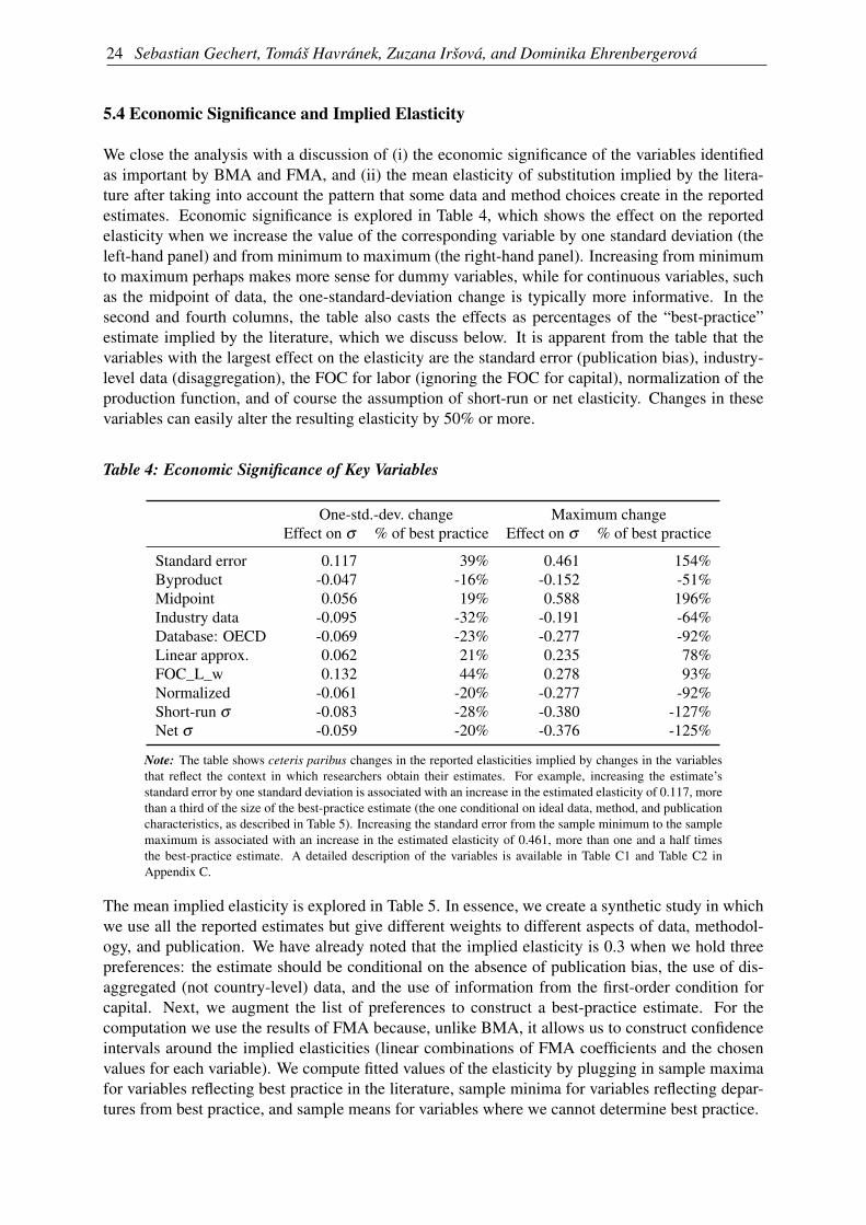
24 Sebastian Gechert, Tomáš Havránek, Zuzana Iršová, and Dominika Ehrenbergerová
5.4 Economic Significance and Implied Elasticity
We close the analysis with a discussion of (i) the economic significance of the variables identifiedas important by BMA and FMA, and (ii) the mean elasticity of substitution implied by the litera-ture after taking into account the pattern that some data and method choices create in the reportedestimates. Economic significance is explored in Table 4, which shows the effect on the reportedelasticity when we increase the value of the corresponding variable by one standard deviation (theleft-hand panel) and from minimum to maximum (the right-hand panel). Increasing from minimumto maximum perhaps makes more sense for dummy variables, while for continuous variables, suchas the midpoint of data, the one-standard-deviation change is typically more informative. In thesecond and fourth columns, the table also casts the effects as percentages of the “best-practice”estimate implied by the literature, which we discuss below. It is apparent from the table that thevariables with the largest effect on the elasticity are the standard error (publication bias), industry-level data (disaggregation), the FOC for labor (ignoring the FOC for capital), normalization of theproduction function, and of course the assumption of short-run or net elasticity. Changes in thesevariables can easily alter the resulting elasticity by 50% or more.
Table 4: Economic Significance of Key Variables
One-std.-dev. change Maximum changeEffect on σ % of best practice Effect on σ % of best practice
Standard error 0.117 39% 0.461 154%Byproduct -0.047 -16% -0.152 -51%Midpoint 0.056 19% 0.588 196%Industry data -0.095 -32% -0.191 -64%Database: OECD -0.069 -23% -0.277 -92%Linear approx. 0.062 21% 0.235 78%FOC_L_w 0.132 44% 0.278 93%Normalized -0.061 -20% -0.277 -92%Short-run σ -0.083 -28% -0.380 -127%Net σ -0.059 -20% -0.376 -125%
Note: The table shows ceteris paribus changes in the reported elasticities implied by changes in the variablesthat reflect the context in which researchers obtain their estimates. For example, increasing the estimate’sstandard error by one standard deviation is associated with an increase in the estimated elasticity of 0.117, morethan a third of the size of the best-practice estimate (the one conditional on ideal data, method, and publicationcharacteristics, as described in Table 5). Increasing the standard error from the sample minimum to the samplemaximum is associated with an increase in the estimated elasticity of 0.461, more than one and a half timesthe best-practice estimate. A detailed description of the variables is available in Table C1 and Table C2 inAppendix C.
The mean implied elasticity is explored in Table 5. In essence, we create a synthetic study in whichwe use all the reported estimates but give different weights to different aspects of data, methodol-ogy, and publication. We have already noted that the implied elasticity is 0.3 when we hold threepreferences: the estimate should be conditional on the absence of publication bias, the use of dis-aggregated (not country-level) data, and the use of information from the first-order condition forcapital. Next, we augment the list of preferences to construct a best-practice estimate. For thecomputation we use the results of FMA because, unlike BMA, it allows us to construct confidenceintervals around the implied elasticities (linear combinations of FMA coefficients and the chosenvalues for each variable). We compute fitted values of the elasticity by plugging in sample maximafor variables reflecting best practice in the literature, sample minima for variables reflecting depar-tures from best practice, and sample means for variables where we cannot determine best practice.

Death to the Cobb-Douglas Production Function? A Quantitative Survey of the Capital-LaborSubstitution Elasticity 25
We prefer large studies using newer data, so we plug in sample maxima for the number of obser-vations and the midpoint of data. We prefer a system of production function together with FOCsfor both capital and labor, tied with normalization and cross-equation restrictions. We also preferthe use of factor-augmenting technological change and joint estimation of equations by Zellner’smethod instead of OLS. As for the publication characteristics, we prefer studies that are highlycited and published in top journals. In contrast, we do not prefer linear approximation, byproductestimates, elasticities that are supposed to be long-run but are not properly adjusted, and partialelasticities: we plug in zero for these variables. We do not have any strong opinion on the var-ious sources of data or data dimension (whether time series or cross-sectional studies should beused, what data frequency should be employed). Thus, next to the central “best-practice” estimatewe generate multiple estimates for these data and method choices. We also show implied elastici-ties for aggregated, country-level data, often used in the literature, and for short-run elasticity, netelasticity, and the use of a system of FOCs without a production function.
Table 5: Results from a Synthetic Study
Implied elasticity 95% confidence interval
Best practice 0.30 (-0.01, 0.60)Short-run -0.11 (-0.38, 0.15)Net σ -0.02 (-0.30, 0.25)Country-level data 0.50 (0.18, 0.81)Quarterly data 0.42 (0.08, 0.76)Time series 0.25 (-0.10, 0.60)Cross-sections 0.32 (0.07, 0.56)System of FOCs 0.35 (0.07, 0.64)
Note: The table shows mean estimates of the elasticity of substitution conditional on data, method, and publica-tion characteristics. The exercise is akin to a synthetic study that uses all information reported in the literaturebut puts more weight on selected aspects of study design. The result in the first column is conditional on ourdefinition of best practice (see the main text for details). The remaining rows change one aspect in the definitionof best practice: for example the second row shows the result for short-run instead of long-run estimates.
The results, shown in Table 5, illustrate the high degree of uncertainty that such an exercise entails:the 95% confidence intervals for all estimates are approximately 0.6 wide. Our central estimate isstill 0.3, which means that other aspects of best practice (on top of the three preferences made inthe beginning) cancel each other out—even though now the estimate becomes barely statisticallysignificantly different from zero at the 5% level. But even such a conservative estimation rejectsthe Cobb-Douglas specification in all cases. The implied short-run and net elasticities are closeto zero. When one prefers quarterly data instead of showing equal treatment to estimates derivedfrom data of different frequencies, the implied estimate increases to 0.4. A preference for timeseries data, cross-sectional data, or a system of FOCs without a production function would resultin a smaller change in the elasticity. Even a preference for country-level data would only take theimplied estimate to 0.5, with the upper bound of the 95% confidence interval at 0.8, making theresult safely inconsistent with the Cobb-Douglas specification.4
4 Different researchers may have different opinions on what constitutes best practice: even though we prefer to usedisaggregated data in general, central bankers’ structural models are mostly calibrated on country-level, quarterlydata, so these dimensions may be more relevant for them. Even in the case of combining quarterly data andcountry-level data, the best-practice estimate yields a maximum of 0.62. Similarly, one may be interested inimplied elasticities for different countries. For instance, the results for the US and developed European countriesare slightly higher than those for other countries, with a baseline implied elasticity of 0.42 and 0.48. Deeperexamination of cross-country differences in substitution elasticity is a topic of our current follow-up project.

26 Sebastian Gechert, Tomáš Havránek, Zuzana Iršová, and Dominika Ehrenbergerová
6. Concluding Remarks
The Cobb-Douglas production function contradicts the data. This is the result we obtain after ana-lyzing 3,186 estimates of the capital-labor substitution elasticity reported in 121 published studies.When we give the same weight to all the different approaches used to identify the elasticity, we findthat the value most representative of the literature is 0.5, tightly estimated with the upper boundof the 95% confidence interval at 0.6. The representative value corresponds to the mean reportedelasticity corrected for publication bias, a phenomenon that has not previously been addressed inthe vast literature on the elasticity of substitution. The representative estimate further shrinks to0.3 when one imposes the restrictions that identification must come from industry-level instead ofaggregated, country-level data and that information from the first-order condition for capital mustbe considered instead of ignored. The representative estimate stays at 0.3 when we control for 71aspects of study design and select a best-practice value for each aspect (plugging in mean valueswhere no reasonable choice can be made). Such best-practice elasticity is imprecisely estimated,with the upper bound of the 95% confidence interval still at 0.6. Other researchers will have differentopinions on what constitutes best practice. But no matter the preferences, after acknowledging pub-lication bias, the Cobb-Douglas production function with the elasticity at 1 becomes indefensible inthe light of empirical evidence.
We are not the first to highlight the disconnect between the Cobb-Douglas specification commonlyused in macroeconomic models and the empirical literature estimating the elasticity of substitution.Chirinko (2008) and Knoblach et al. (2019) provide useful surveys of portions of the literature,and both studies suggest that the Cobb-Douglas production function is not backed by the availableevidence. We argue that after controlling for publication bias and model uncertainty the true valueof the elasticity decreases even more and the case against Cobb-Douglas strengthens.
Three caveats to the precise value of our central estimate, 0.3, are in order. First, the elasticitiesthat we collect are unlikely to be independent, because they are frequently derived from the sameor similar datasets. We partially address this problem by clustering standard errors at both the studyand country level when controlling for publication bias and additionally compute wild bootstrapconfidence intervals. Second, the value of 0.3 is a mean estimate and does not necessarily fit allsituations and calibrations. While we do not find much evidence of systematic differences in theelasticity across countries and industries, in a companion project we are currently working on a moredetailed examination of structural determinants of the elasticity. Third, we do our best to include allpublished studies estimating the elasticity of substitution, but we still might have missed some. Suchan omission will not affect our results much as long as it remains random. We experimented withrandomly omitting 50% of our data set, and the main findings continue to hold in such simulations.
Death to the Cobb-Douglas Production Function? A Quantitative Survey of the Capital-LaborSubstitution Elasticity 27
References
AMINI, S. M. AND C. F. PARMETER (2012): “Comparison of Model Averaging Techniques:Assessing Growth Determinants.” Journal of Applied Econometrics, 27(5):870–876.
ANDREWS, I. AND M. KASY (2019): “Identification of and Correction for Publication Bias.”Americal Economic Review, 109(8):2766–2794.
ANTRAS, P. (2004): “Is the US Aggregate Production Function Cobb-Douglas? New Estimates ofthe Elasticity of Substitution.” Contributions in Macroeconomics, 4(1):1–36.
ARROW, K. J., H. B. CHENERY, B. S. MINHAS, AND R. M. SOLOW (1961): “Capital-LaborSubstitution and Economic Efficiency.” Review of Economics and Statistics, 43(3):225–250.
ASHENFELTER, O. AND M. GREENSTONE (2004): “Estimating the Value of a Statistical Life:The Importance of Omitted Variables and Publication Bias.” American Economic Review,94(2):454–460.
BAKER, R. D. AND D. JACKSON (2013): “Meta-Analysis Inside and Outside Particle Physics:Two Traditions that Should Converge?.” Research Synthesis Methods, 4(2):109–124.
BEHRMAN, J. R. (1972): “Sectoral Elasticities of Substitution between Capital and Labor in aDeveloping Economy: Times Series Analysis in the Case of Postwar Chile.” Econometrica,40(2):311–326.
BERNDT, E. R. (1976): “Reconciling Alternative Estimates of the Elasticity of Substitution.”Review of Economics and Statistics, 58(1):59–68.
BOM, P. R. D. AND H. RACHINGER (2019): “A Kinked Meta-Regression Model for PublicationBias Correction.” Research Synthesis Methods, 10(4):497–514.
BOX, G. E. AND D. R. COX (1964): “An Analysis of Transformations.” Journal of the RoyalStatistical Society: Series B (Methodological), 26(2):211–243.
BROWN, M. (1966): “A Measure of the Change in Relative Exploitation of Capital and Labor.”Review of Economics and Statistics, 48(2):182–192.
BRUNO, M. AND J. SACHS (1982): “Input Price Shocks and the Slowdown in Economic Growth:The Case of UK Manufacturing.” Review of Economic Studies, 49(5):679–705.
CAMERON, A. C., J. B. GELBACH, AND D. L. MILLER (2008): “Bootstrap-Based Improvementsfor Inference with Clustered Errors.” Review of Economics and Statistics, 90(3):414–427.
CAMERON, A. C., J. B. GELBACH, AND D. L. MILLER (2011): “Robust Inference with MultiwayClustering.” Journal of Business & Economic Statistics, 29(2):238–249.
CANTORE, C. AND P. LEVINE (2012): “Getting Normalization Right: Dealing with ‘DimensionalConstants’ in Macroeconomics.” Journal of Economic Dynamics and Control, 36(12):1931–1949.
CANTORE, C., M. LEÓN-LEDESMA, P. MCADAM, AND A. WILLMAN (2014): “Shocking Stuff:Technology, Hours, and Factor Substitution.” Journal of the European Economic Associa-tion, 12(1):108–128.
CANTORE, C., P. LEVINE, J. PEARLMAN, AND B. YANG (2015): “CES Technology and BusinessCycle Fluctuations.” Journal of Economic Dynamics and Control, 61:133–151.
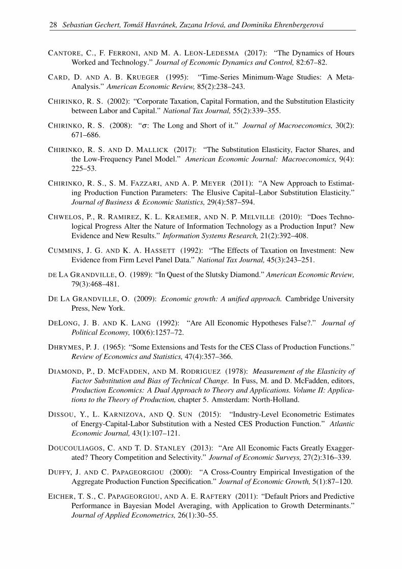
28 Sebastian Gechert, Tomáš Havránek, Zuzana Iršová, and Dominika Ehrenbergerová
CANTORE, C., F. FERRONI, AND M. A. LEON-LEDESMA (2017): “The Dynamics of HoursWorked and Technology.” Journal of Economic Dynamics and Control, 82:67–82.
CARD, D. AND A. B. KRUEGER (1995): “Time-Series Minimum-Wage Studies: A Meta-Analysis.” American Economic Review, 85(2):238–243.
CHIRINKO, R. S. (2002): “Corporate Taxation, Capital Formation, and the Substitution Elasticitybetween Labor and Capital.” National Tax Journal, 55(2):339–355.
CHIRINKO, R. S. (2008): “σ : The Long and Short of it.” Journal of Macroeconomics, 30(2):671–686.
CHIRINKO, R. S. AND D. MALLICK (2017): “The Substitution Elasticity, Factor Shares, andthe Low-Frequency Panel Model.” American Economic Journal: Macroeconomics, 9(4):225–53.
CHIRINKO, R. S., S. M. FAZZARI, AND A. P. MEYER (2011): “A New Approach to Estimat-ing Production Function Parameters: The Elusive Capital–Labor Substitution Elasticity.”Journal of Business & Economic Statistics, 29(4):587–594.
CHWELOS, P., R. RAMIREZ, K. L. KRAEMER, AND N. P. MELVILLE (2010): “Does Techno-logical Progress Alter the Nature of Information Technology as a Production Input? NewEvidence and New Results.” Information Systems Research, 21(2):392–408.
CUMMINS, J. G. AND K. A. HASSETT (1992): “The Effects of Taxation on Investment: NewEvidence from Firm Level Panel Data.” National Tax Journal, 45(3):243–251.
DE LA GRANDVILLE, O. (1989): “In Quest of the Slutsky Diamond.” American Economic Review,79(3):468–481.
DE LA GRANDVILLE, O. (2009): Economic growth: A unified approach. Cambridge UniversityPress, New York.
DELONG, J. B. AND K. LANG (1992): “Are All Economic Hypotheses False?.” Journal ofPolitical Economy, 100(6):1257–72.
DHRYMES, P. J. (1965): “Some Extensions and Tests for the CES Class of Production Functions.”Review of Economics and Statistics, 47(4):357–366.
DIAMOND, P., D. MCFADDEN, AND M. RODRIGUEZ (1978): Measurement of the Elasticity ofFactor Substitution and Bias of Technical Change. In Fuss, M. and D. McFadden, editors,Production Economics: A Dual Approach to Theory and Applications. Volume II: Applica-tions to the Theory of Production, chapter 5. Amsterdam: North-Holland.
DISSOU, Y., L. KARNIZOVA, AND Q. SUN (2015): “Industry-Level Econometric Estimatesof Energy-Capital-Labor Substitution with a Nested CES Production Function.” AtlanticEconomic Journal, 43(1):107–121.
DOUCOULIAGOS, C. AND T. D. STANLEY (2013): “Are All Economic Facts Greatly Exagger-ated? Theory Competition and Selectivity.” Journal of Economic Surveys, 27(2):316–339.
DUFFY, J. AND C. PAPAGEORGIOU (2000): “A Cross-Country Empirical Investigation of theAggregate Production Function Specification.” Journal of Economic Growth, 5(1):87–120.
EICHER, T. S., C. PAPAGEORGIOU, AND A. E. RAFTERY (2011): “Default Priors and PredictivePerformance in Bayesian Model Averaging, with Application to Growth Determinants.”Journal of Applied Econometrics, 26(1):30–55.

Death to the Cobb-Douglas Production Function? A Quantitative Survey of the Capital-LaborSubstitution Elasticity 29
EISNER, R. (1969): “Tax Policy and Investment Behavior: Comment.” American EconomicReview, 59(3):379–388.
EISNER, R. AND M. I. NADIRI (1968): “Investment Behavior and Neo-Classical Theory.” Reviewof Economics and Statistics, 50(3):369–382.
ERCEG, C. J., L. GUERRIERI, AND C. GUST (2008): “Trade Adjustment and the Composition ofTrade.” Journal of Economic Dynamics and Control, 32(8):2622–2650.
FERGUSON, C. E. (1965): “Time-Series Production Functions and Technological Progress inAmerican Manufacturing Industry.” Journal of Political Economy, 73(2):135–147.
FURUKAWA, C. (2019): “Publication Bias under Aggregation Frictions: Theory, Evidence, and aNew Correction Method.” Unpublished paper, MIT.
HALL, R. E. AND D. W. JORGENSON (1967): “Tax Policy and Investment Behavior.” AmericanEconomic Review, 57(3):391–414.
HANSEN, B. E. (2007): “Least Squares Model Averaging.” Econometrica, 75(4):1175–1189.
HEDGES, L. V. (1992): “Modeling Publication Selection Effects in Meta-Analysis.” StatisticalScience, 7(2):246–255.
HICKS, J. R. (1932): “Marginal Productivity and the Principle of Variation.” Economica, (35):79–88.
HUMPHREY, D. B. AND J. R. MORONEY (1975): “Substitution among Capital, Labor, and NaturalResource Products in American Manufacturing.” Journal of Political Economy, 83(1):57–82.
IOANNIDIS, J. P., T. D. STANLEY, AND H. DOUCOULIAGOS (2017): “The Power of Bias inEconomics Research.” Economic Journal, 127(605):236–265.
JORGENSON, D. W. (1963): “Capital Theory and Investment Behavior.” American EconomicReview, 53(2):247–259.
JORGENSON, D. W. (2007): “35 Sector KLEM.” Harvard Dataverse.
KARABARBOUNIS, L. AND B. NEIMAN (2013): “The Global Decline of the Labor Share.” Quar-terly Journal of Economics, 129(1):61–103.
KILPONEN, J., S. ORJASNIEMI, A. RIPATTI, AND F. VERONA (2016): “The Aino 2.0 Model.”Research Discussion Paper 16/2016, Bank of Finland.
KLUMP, R. AND O. DE LA GRANDVILLE (2000): “Economic Growth and the Elasticity ofSubstitution: Two Theorems and Some Suggestions.” American Economic Review, 90(1):282–291.
KLUMP, R., P. MCADAM, AND A. WILLMAN (2007): “Factor Substitution and Factor-Augmenting Technical Progress in the United States: A Normalized Supply-Side SystemApproach.” Review of Economics and Statistics, 89(1):183–192.
KLUMP, R., P. MCADAM, AND A. WILLMAN (2008): “Unwrapping Some Euro Area GrowthPuzzles: Factor Substitution, Productivity and Unemployment.” Journal of Macroeco-nomics, 30(2):645–666.
KLUMP, R., P. MCADAM, AND A. WILLMAN (2012): “The Normalized CES Production Func-tion: Theory and Empirics.” Journal of Economic Surveys, 26(5):769–799.
30 Sebastian Gechert, Tomáš Havránek, Zuzana Iršová, and Dominika Ehrenbergerová
KMENTA, J. (1967): “On Estimation of the CES Production Function.” International EconomicReview, 8(2):180–189.
KNOBLACH, M., M. ROSSLER, AND P. ZWERSCHKE (2019): “The Elasticity of SubstitutionBetween Capital and Labour in the US Economy: A Meta-Regression Analysis.” OxfordBulletin of Economic and Statistics, 82(1):62–82.
KRUSELL, P., L. E. OHANIAN, J.-V. ROOS-RULL, AND G. L. VIOLANTE (2000): “Capital-Skill Complementarity and Inequality: A Macroeconomic Analysis.” Econometrica, 68(5):1029–1053.
LEÓN-LEDESMA, M. A., P. MCADAM, AND A. WILLMAN (2010): “Identifying the Elasticity ofSubstitution with Biased Technical Change.” American Economic Review, 100(4):1330–57.
LOVELL, C. K. (1973): “CES and VES Production Functions in a Cross-Section Context.” Journalof Political Economy, 81(3):705–720.
MADIGAN, D. AND J. YORK (1995): “Graphical Models for Discrete Data.” InternationalStatistical Review, 63(2):215–232.
MCCLOSKEY, D. N. AND S. T. ZILIAK (2019): “What Quantitative Methods Should We Teach toGraduate Students? A Comment on Swann’s “Is Precise Econometrics an Illusion?”.” TheJournal of Economic Education, 50(4):356–361.
NERLOVE, M. (1967): Recent Empirical Studies of the CES and Related Production Functions.In Brown, M., editors, The Theory and Empirical Analysis of Production, pages 55–136.NBER.
PIKETTY, T. (2014): Capital in the 21st Century. Harvard University Press, Cambridge, MA.
ROBINSON, J. (1933): Economics of Imperfect Competition. The Macmillan Company, NewYork.
ROGNLIE, M. (2014): “A Note on Piketty and Diminishing Returns to Capital.” Unpublishedpaper, MIT.
ROODMAN, D. (2019): “BOOTTEST: Stata Module to Provide Fast Execution of the Wild Boot-strap with Null Imposed.” Statistical Software Components S458121, Boston College De-partment of Economics.
RUSNAK, M., T. HAVRANEK, AND R. HORVATH (2013): “How to Solve the Price Puzzle? AMeta-Analysis.” Journal of Money, Credit and Banking, 45(1):37–70.
SEMIENIUK, G. (2017): “Piketty’s Elasticity of Substitution: A Critique.” Review of PoliticalEconomy, 29(1):64–79.
SMITH, J. (2008): “That Elusive Elasticity and the Ubiquitous Bias: Is Panel Data a Panacea?.”Journal of Macroeconomics, 30(2):760–779.
SOLOW, R. M. (1956): “A Contribution to the Theory of Economic Growth.” Quarterly Journalof Economics, 70(1):65–94.
STANLEY, T., S. B. JARRELL, AND H. DOUCOULIAGOS (2010): “Could it Be Better to Discard90% of the Data? A Statistical Paradox.” American Statistician, 64(1):70–77.
STANLEY, T. D. (2005): “Beyond Publication Bias.” Journal of Economic Surveys, 19(3):309–345.

Death to the Cobb-Douglas Production Function? A Quantitative Survey of the Capital-LaborSubstitution Elasticity 31
STANLEY, T. D. AND H. DOUCOULIAGOS (2010): “Picture This: A Simple Graph that RevealsMuch Ado about Research.” Journal of Economic Surveys, 24(1):170–191.
STANLEY, T. D. AND H. DOUCOULIAGOS (2017): “Neither Fixed nor Random: Weighted LeastSquares Meta-Regression.” Research Synthesis Methods, 8(1):19–42.
STEEL, M. F. J. (2019): “Model Averaging and its Use in Economics.” Journal of EconomicLiterature, forthcoming.
THURSBY, J. G. AND C. K. LOVELL (1978): “An Investigation of the Kmenta Approximation tothe CES Function.” International Economic Review, 19(2):363–377.
TURNOVSKY, S. J. (2002): “Intertemporal and Intratemporal Substitution, and the Speed of Con-vergence in the Neoclassical Growth Model.” Journal of Economic Dynamics and Control,26(9-10):1765–1785.
VAN DER WERF, E. (2008): “Production Functions for Climate Policy Modeling: An EmpiricalAnalysis.” Energy Economics, 30(6):2964–2979.
YOUNG, A. T. (2013): “US Elasticities of Substitution and Factor Augmentation at the IndustryLevel.” Macroeconomic Dynamics, 17(4):861–897.
ZAREMBKA, P. (1970): “On the Empirical Relevance of the CES Production Function.” Reviewof Economics and Statistics, 52(1):47–53.
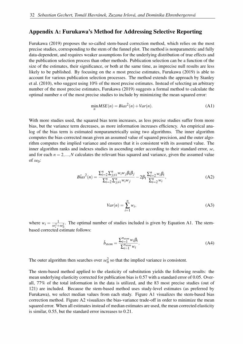
32 Sebastian Gechert, Tomáš Havránek, Zuzana Iršová, and Dominika Ehrenbergerová
Appendix A: Furukawa’s Method for Addressing Selective Reporting
Furukawa (2019) proposes the so-called stem-based correction method, which relies on the mostprecise studies, corresponding to the stem of the funnel plot. The method is nonparametric and fullydata-dependent, and requires weaker assumptions for the underlying distribution of true effects andthe publication selection process than other methods. Publication selection can be a function of thesize of the estimates, their significance, or both at the same time, as imprecise null results are lesslikely to be published. By focusing on the n most precise estimates, Furukawa (2019) is able toaccount for various publication selection processes. The method extends the approach by Stanleyet al. (2010), who suggest using 10% of the most precise estimates. Instead of selecting an arbitrarynumber of the most precise estimates, Furukawa (2019) suggests a formal method to calculate theoptimal number n of the most precise studies to include by minimizing the mean squared error:
minn
MSE(n) = Bias2(n)+Var(n). (A1)
With more studies used, the squared bias term increases, as less precise studies suffer from morebias, but the variance term decreases, as more information increases efficiency. An empirical ana-log of the bias term is estimated nonparametrically using two algorithms. The inner algorithmcomputes the bias-corrected mean given an assumed value of squared precision, and the outer algo-rithm computes the implied variance and ensures that it is consistent with its assumed value. Theinner algorithm ranks and indexes studies in ascending order according to their standard error, se,and for each n = 2, ...,N calculates the relevant bias squared and variance, given the assumed valueof se0:
˜Bias2(n) =
∑ni=2 ∑
nj 6=i wiw jβiβ j
∑ni=2 ∑
nj 6=i wiw j
−2β1∑
ni=2 wiβi
∑ni=2 wi
, (A2)
Var(n) =n
∑i=1
wi, (A3)
where wi =1
se2i +se2
0. The optimal number of studies included is given by Equation A1. The stem-
based corrected estimate follows:
bstem =∑
nstemi=1 wiβi
∑nstemi=1 wi
. (A4)
The outer algorithm then searches over se20 so that the implied variance is consistent.
The stem-based method applied to the elasticity of substitution yields the following results: themean underlying elasticity corrected for publication bias is 0.57 with a standard error of 0.05. Over-all, 77% of the total information in the data is utilized, and the 83 most precise studies (out of121) are included. Because the stem-based method uses study-level estimates (as preferred byFurukawa), we select median values from each study. Figure A1 visualizes the stem-based biascorrection method. Figure A2 visualizes the bias-variance trade-off in order to minimize the meansquared error. When all estimates instead of median estimates are used, the mean corrected elasticityis similar, 0.55, but the standard error increases to 0.21.
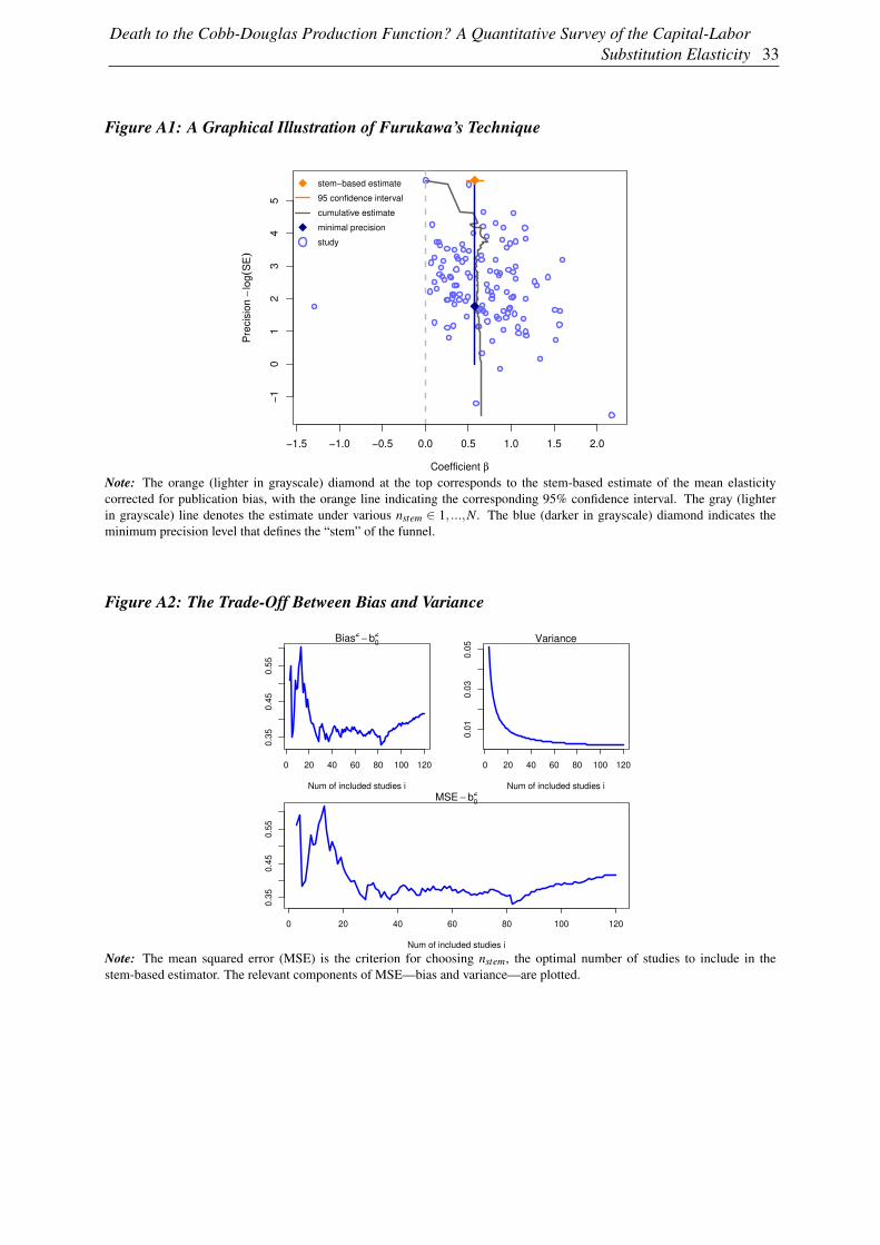
Death to the Cobb-Douglas Production Function? A Quantitative Survey of the Capital-LaborSubstitution Elasticity 33
Figure A1: A Graphical Illustration of Furukawa’s Technique
−1.5 −1.0 −0.5 0.0 0.5 1.0 1.5 2.0
−1
01
23
45
Coefficient β
Pre
cis
ion −
log(S
E)
stem−based estimate
95 confidence interval
cumulative estimate
minimal precision
study
Note: The orange (lighter in grayscale) diamond at the top corresponds to the stem-based estimate of the mean elasticitycorrected for publication bias, with the orange line indicating the corresponding 95% confidence interval. The gray (lighterin grayscale) line denotes the estimate under various nstem ∈ 1, ...,N. The blue (darker in grayscale) diamond indicates theminimum precision level that defines the “stem” of the funnel.
Figure A2: The Trade-Off Between Bias and Variance
0 20 40 60 80 100 120
0.3
50.4
50.5
5
Bias2
− b0
2
Num of included studies i
0 20 40 60 80 100 120
0.0
10.0
30.0
5
Variance
Num of included studies i
0 20 40 60 80 100 120
0.3
50.4
50.5
5
MSE − b0
2
Num of included studies i
Note: The mean squared error (MSE) is the criterion for choosing nstem, the optimal number of studies to include in thestem-based estimator. The relevant components of MSE—bias and variance—are plotted.

34 Sebastian Gechert, Tomáš Havránek, Zuzana Iršová, and Dominika Ehrenbergerová
Appendix B: Andrews and Kasy’s Method for Addressing Selective Re-porting
Andrews and Kasy (2019) introduce two approaches for the identification of publication selection:the first one based on data from replication studies and the second one tailored for meta-analysis.They show that the meta-analysis approach delivers results similar to the approach based on replica-tions. In the absence of publication bias, the distribution of the estimates from imprecise studies canbe written as the distribution for precise studies plus noise; deviations from this form identify condi-tional publication probabilities. Andrews and Kasy (2019) identify publication probability similarlyto Hedges (1992) using maximum likelihood: the conditional publication probability, p(·), is a stepfunction with jumps at conventional critical values of the p-value.
When applied to our data, the method by Andrews and Kasy (2019) yields the following results.The bias-corrected estimate is 0.43 with a standard error of 0.017. We impose a cut-off at zero,that is, we compare the publication probability of negative vs. positive estimates regardless of theirsignificance. (Allowing for other jumps in publication probability would yield even smaller esti-mates of the mean elasticity corrected for publication bias.) Our results also suggest that positiveestimates are six times more likely to be selected for publication than negative estimates (Table B1).In the case of the elasticity of substitution, publication selection based on statistical significance isapparently less pronounced than selection based on the sign of the estimate, as suggested by theright panel of Figure B1.
Figure B1: A Graphical Illustration of Andrews and Kasy’s (2019) Estimator
0.0
0.1
0.2
0.3
0.4
−3 0 3 6
X Σ
Den
sity
0
2
4
6
8
−5.0 −2.5 0.0 2.5 5.0
X
Σ
significant
FALSETRUE
Note: The solid gray lines mark t-statistic equal to 1.96 in absolute value; the dashed gray line marks t-statistic equal to 2.33in absolute value. We observe a jump at t-statistic equal to zero and then also jumps at conventional significance levels. Theright-hand figure plots estimates X and their standard errors Σ; the gray line marks 1.96 in absolute value. Even though weobserve discontinuity at the t-statistic corresponding to the 5% significance level, the right panel shows publication selectionbased on significance is not absolute, as some insignificant estimates (gray points) are reported.
Table B1: Results of Andrews and Kasy’s (2019) Estimator
θ τ DF βp
Estimate 0.430 0.489 12.809 0.158Standard error 0.017 0.012 0.707 0.019
Note: θ denotes the bias-corrected mean effect, τ is a scale parameter, DF are degrees of freedom. βp is a publicationprobability measured relative to the omitted category, in our case positive estimates. An estimate of 0.158 therefore impliesthat negative results are 15.8% as likely to be published as positive ones.
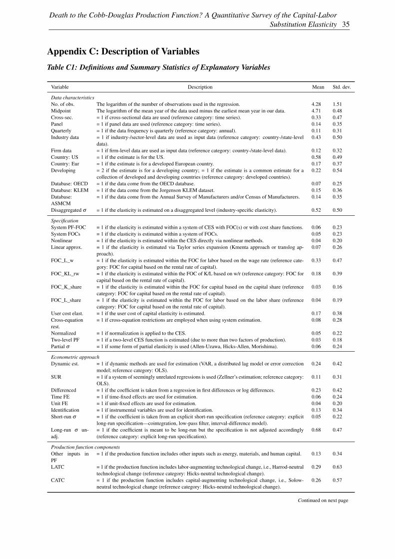
Death to the Cobb-Douglas Production Function? A Quantitative Survey of the Capital-LaborSubstitution Elasticity 35
Appendix C: Description of VariablesTable C1: Definitions and Summary Statistics of Explanatory Variables
Variable Description Mean Std. dev.
Data characteristicsNo. of obs. The logarithm of the number of observations used in the regression. 4.28 1.51Midpoint The logarithm of the mean year of the data used minus the earliest mean year in our data. 4.71 0.48Cross-sec. = 1 if cross-sectional data are used (reference category: time series). 0.33 0.47Panel = 1 if panel data are used (reference category: time series). 0.14 0.35Quarterly = 1 if the data frequency is quarterly (reference category: annual). 0.11 0.31Industry data = 1 if industry-/sector-level data are used as input data (reference category: country-/state-level
data).0.43 0.50
Firm data = 1 if firm-level data are used as input data (reference category: country-/state-level data). 0.12 0.32Country: US = 1 if the estimate is for the US. 0.58 0.49Country: Eur = 1 if the estimate is for a developed European country. 0.17 0.37Developing = 2 if the estimate is for a developing country; = 1 if the estimate is a common estimate for a
collection of developed and developing countries (reference category: developed countries).0.22 0.54
Database: OECD = 1 if the data come from the OECD database. 0.07 0.25Database: KLEM = 1 if the data come from the Jorgenson KLEM dataset. 0.15 0.36Database:ASMCM
= 1 if the data come from the Annual Survey of Manufacturers and/or Census of Manufacturers. 0.14 0.35
Disaggregated σ = 1 if the elasticity is estimated on a disaggregated level (industry-specific elasticity). 0.52 0.50
SpecificationSystem PF-FOC = 1 if the elasticity is estimated within a system of CES with FOC(s) or with cost share functions. 0.06 0.23System FOCs = 1 if the elasticity is estimated within a system of FOCs. 0.05 0.23Nonlinear = 1 if the elasticity is estimated within the CES directly via nonlinear methods. 0.04 0.20Linear approx. = 1 if the elasticity is estimated via Taylor series expansion (Kmenta approach or translog ap-
proach).0.07 0.26
FOC_L_w = 1 if the elasticity is estimated within the FOC for labor based on the wage rate (reference cate-gory: FOC for capital based on the rental rate of capital).
0.33 0.47
FOC_KL_rw = 1 if the elasticity is estimated within the FOC of K/L based on w/r (reference category: FOC forcapital based on the rental rate of capital).
0.18 0.39
FOC_K_share = 1 if the elasticity is estimated within the FOC for capital based on the capital share (referencecategory: FOC for capital based on the rental rate of capital).
0.03 0.16
FOC_L_share = 1 if the elasticity is estimated within the FOC for labor based on the labor share (referencecategory: FOC for capital based on the rental rate of capital).
0.04 0.19
User cost elast. = 1 if the user cost of capital elasticity is estimated. 0.17 0.38Cross-equationrest.
= 1 if cross-equation restrictions are employed when using system estimation. 0.08 0.28
Normalized = 1 if normalization is applied to the CES. 0.05 0.22Two-level PF = 1 if a two-level CES function is estimated (due to more than two factors of production). 0.03 0.18Partial σ = 1 if some form of partial elasticity is used (Allen-Uzawa, Hicks-Allen, Morishima). 0.06 0.24
Econometric approachDynamic est. = 1 if dynamic methods are used for estimation (VAR, a distributed lag model or error correction
model; reference category: OLS).0.24 0.42
SUR = 1 if a system of seemingly unrelated regressions is used (Zellner’s estimation; reference category:OLS).
0.11 0.31
Differenced = 1 if the coefficient is taken from a regression in first differences or log differences. 0.23 0.42Time FE = 1 if time-fixed effects are used for estimation. 0.06 0.24Unit FE = 1 if unit-fixed effects are used for estimation. 0.04 0.20Identification = 1 if instrumental variables are used for identification. 0.13 0.34Short-run σ = 1 if the coefficient is taken from an explicit short-run specification (reference category: explicit
long-run specification—cointegration, low-pass filter, interval-difference model).0.05 0.22
Long-run σ un-adj.
= 1 if the coefficient is meant to be long-run but the specification is not adjusted accordingly(reference category: explicit long-run specification).
0.68 0.47
Production function componentsOther inputs inPF
= 1 if the production function includes other inputs such as energy, materials, and human capital. 0.13 0.34
LATC = 1 if the production function includes labor-augmenting technological change, i.e., Harrod-neutraltechnological change (reference category: Hicks-neutral technological change).
0.29 0.63
CATC = 1 if the production function includes capital-augmenting technological change, i.e., Solow-neutral technological change (reference category: Hicks-neutral technological change).
0.26 0.57
Continued on next page
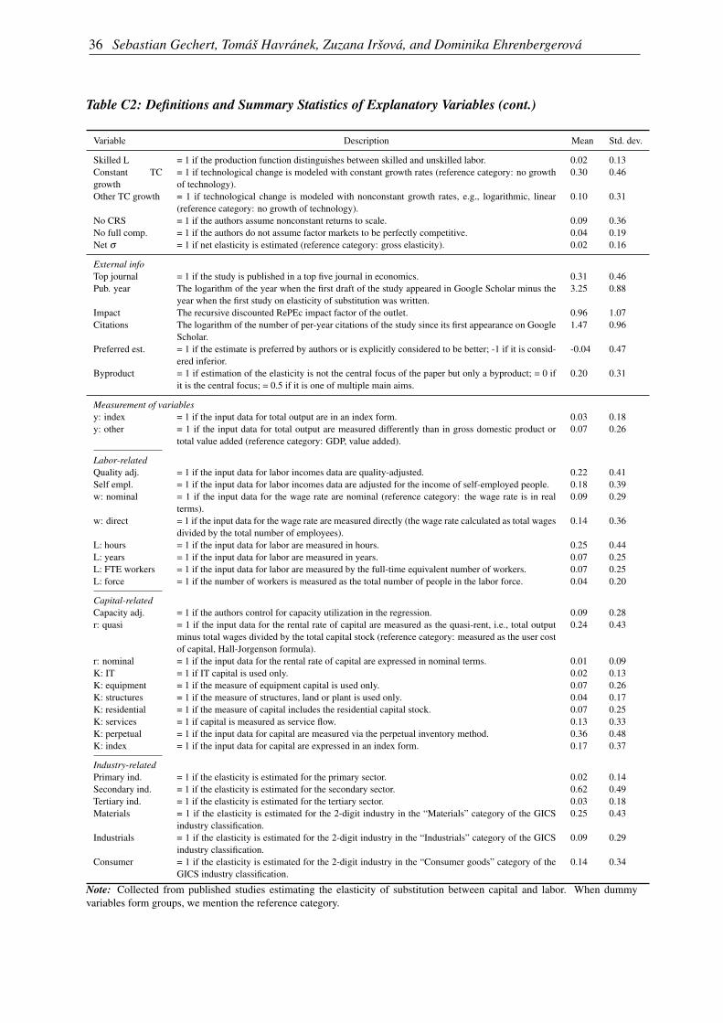
36 Sebastian Gechert, Tomáš Havránek, Zuzana Iršová, and Dominika Ehrenbergerová
Table C2: Definitions and Summary Statistics of Explanatory Variables (cont.)
Variable Description Mean Std. dev.
Skilled L = 1 if the production function distinguishes between skilled and unskilled labor. 0.02 0.13Constant TCgrowth
= 1 if technological change is modeled with constant growth rates (reference category: no growthof technology).
0.30 0.46
Other TC growth = 1 if technological change is modeled with nonconstant growth rates, e.g., logarithmic, linear(reference category: no growth of technology).
0.10 0.31
No CRS = 1 if the authors assume nonconstant returns to scale. 0.09 0.36No full comp. = 1 if the authors do not assume factor markets to be perfectly competitive. 0.04 0.19Net σ = 1 if net elasticity is estimated (reference category: gross elasticity). 0.02 0.16
External infoTop journal = 1 if the study is published in a top five journal in economics. 0.31 0.46Pub. year The logarithm of the year when the first draft of the study appeared in Google Scholar minus the
year when the first study on elasticity of substitution was written.3.25 0.88
Impact The recursive discounted RePEc impact factor of the outlet. 0.96 1.07Citations The logarithm of the number of per-year citations of the study since its first appearance on Google
Scholar.1.47 0.96
Preferred est. = 1 if the estimate is preferred by authors or is explicitly considered to be better; -1 if it is consid-ered inferior.
-0.04 0.47
Byproduct = 1 if estimation of the elasticity is not the central focus of the paper but only a byproduct; = 0 ifit is the central focus; = 0.5 if it is one of multiple main aims.
0.20 0.31
Measurement of variablesy: index = 1 if the input data for total output are in an index form. 0.03 0.18y: other = 1 if the input data for total output are measured differently than in gross domestic product or
total value added (reference category: GDP, value added).0.07 0.26
Labor-relatedQuality adj. = 1 if the input data for labor incomes data are quality-adjusted. 0.22 0.41Self empl. = 1 if the input data for labor incomes data are adjusted for the income of self-employed people. 0.18 0.39w: nominal = 1 if the input data for the wage rate are nominal (reference category: the wage rate is in real
terms).0.09 0.29
w: direct = 1 if the input data for the wage rate are measured directly (the wage rate calculated as total wagesdivided by the total number of employees).
0.14 0.36
L: hours = 1 if the input data for labor are measured in hours. 0.25 0.44L: years = 1 if the input data for labor are measured in years. 0.07 0.25L: FTE workers = 1 if the input data for labor are measured by the full-time equivalent number of workers. 0.07 0.25L: force = 1 if the number of workers is measured as the total number of people in the labor force. 0.04 0.20
Capital-relatedCapacity adj. = 1 if the authors control for capacity utilization in the regression. 0.09 0.28r: quasi = 1 if the input data for the rental rate of capital are measured as the quasi-rent, i.e., total output
minus total wages divided by the total capital stock (reference category: measured as the user costof capital, Hall-Jorgenson formula).
0.24 0.43
r: nominal = 1 if the input data for the rental rate of capital are expressed in nominal terms. 0.01 0.09K: IT = 1 if IT capital is used only. 0.02 0.13K: equipment = 1 if the measure of equipment capital is used only. 0.07 0.26K: structures = 1 if the measure of structures, land or plant is used only. 0.04 0.17K: residential = 1 if the measure of capital includes the residential capital stock. 0.07 0.25K: services = 1 if capital is measured as service flow. 0.13 0.33K: perpetual = 1 if the input data for capital are measured via the perpetual inventory method. 0.36 0.48K: index = 1 if the input data for capital are expressed in an index form. 0.17 0.37
Industry-relatedPrimary ind. = 1 if the elasticity is estimated for the primary sector. 0.02 0.14Secondary ind. = 1 if the elasticity is estimated for the secondary sector. 0.62 0.49Tertiary ind. = 1 if the elasticity is estimated for the tertiary sector. 0.03 0.18Materials = 1 if the elasticity is estimated for the 2-digit industry in the “Materials” category of the GICS
industry classification.0.25 0.43
Industrials = 1 if the elasticity is estimated for the 2-digit industry in the “Industrials” category of the GICSindustry classification.
0.09 0.29
Consumer = 1 if the elasticity is estimated for the 2-digit industry in the “Consumer goods” category of theGICS industry classification.
0.14 0.34
Note: Collected from published studies estimating the elasticity of substitution between capital and labor. When dummyvariables form groups, we mention the reference category.
Death to the Cobb-Douglas Production Function? A Quantitative Survey of the Capital-LaborSubstitution Elasticity 37
Appendix D: Robustness ChecksTable D1: Results of Frequentist Model Averaging
Coef. Std. er. p-value
Standard error 0.557 0.042 0.000
Data characteristicsNo. of obs. 0.011 0.012 0.326Midpoint 0.103 0.022 0.000Cross-sec. 0.069 0.029 0.016Panel 0.193 0.042 0.000Quarterly 0.135 0.042 0.001Firm data -0.160 0.040 0.000Industry data -0.198 0.026 0.000Country: US 0.121 0.031 0.000Country: Eur 0.180 0.030 0.000Developing 0.019 0.019 0.333Database: ASM,CM -0.031 0.037 0.402Database: OECD -0.301 0.044 0.000Database: KLEM -0.092 0.046 0.047Disaggregated σ 0.043 0.024 0.077
SpecificationSystem PF+FOC -0.111 0.059 0.061System FOCs -0.057 0.050 0.258Nonlinear -0.016 0.061 0.796Linear approx. 0.268 0.050 0.000FOC_L_w 0.324 0.032 0.000FOC_KL_rw 0.007 0.032 0.832FOC_K_share 0.226 0.063 0.000FOC_L_share 0.251 0.048 0.000Cross-eq. restr. 0.071 0.048 0.140Normalized -0.248 0.051 0.000Two-level PF -0.023 0.070 0.743Partial sigma 0.130 0.055 0.018User cost. elast. -0.373 0.042 0.000
Econometric approachDynamic est. -0.005 0.029 0.854SUR -0.105 0.032 0.001Identification 0.046 0.026 0.077Differenced -0.096 0.027 0.000Time FE -0.009 0.040 0.830Unit FE 0.067 0.043 0.116Short-run -0.410 0.040 0.000Long-run unadj. -0.011 0.026 0.681
Production function componentsOther inputs in PF -0.137 0.044 0.002CATC -0.003 0.026 0.904LATC -0.041 0.024 0.088Skilled L 0.076 0.059 0.199Constant TC growth -0.032 0.025 0.191Other TC growth 0.108 0.035 0.002No CRS -0.003 0.022 0.905No full comp. -0.022 0.042 0.598Net sigma -0.320 0.056 0.000
Publication characteristicsTop journal -0.085 0.025 0.001Pub. year 0.032 0.015 0.038Citations 0.037 0.011 0.001Preferred 0.027 0.016 0.093Byproduct -0.130 0.032 0.000(Intercept) -0.123 0.130 0.342
Observations 3,186
Note: Our frequentist model averaging (FMA) exercise employs Mallow’s weights (Hansen, 2007) and the orthogonalizationof the covariate space suggested by Amini and Parmeter (2012). Dark gray color denotes variables that are deemed importantalso in the BMA exercise. Light gray color denotes variables that are deemed important in the FMA but not the BMA exercise.

38 Sebastian Gechert, Tomáš Havránek, Zuzana Iršová, and Dominika Ehrenbergerová
Figure D1: Model Inclusion in Bayesian Model Averaging, Weighted by the Inverse of the Num-ber of Estimates per Study
0 0.06 0.14 0.2 0.26 0.32 0.38 0.44 0.5 0.55 0.6 0.66 0.72 0.78 0.84
St. errorMidpoint
Industry data Country: US Country: Eur
DevelopingFOC_L_w
FOC_L_share User cost. elast.
Dynamic est. Time FE
Short−run Citations
Net sigmaUnit FE
LATCNo full comp.
Linear approx. System PF+FOC
Two−level PF Preferred
Other TC growth FOC_KL_rw
NonlinearPub. year
Constant TC growth Database: KLEM
QuarterlyCross−sec.
Ind. disaggregated FOC_K_share
SUR ByproductNo. of obs. Normalized
No CRSCross−eq. restr.
System FOCs Partial sigma
Long−run unadj. Firm data
DifferencedTop journal
Other inputs in PF Skilled L
CATCDatabase: OECD
Database: ASM,CM Panel
Identification
Note: The response variable is the estimate of the elasticity of substitution. Columns denote individual models; variablesare sorted by posterior inclusion probability in descending order. The horizontal axis denotes cumulative posterior modelprobabilities; only the 5,000 best models are shown. Blue color (darker in grayscale) = the variable is included and theestimated sign is positive. Red color (lighter in grayscale) = the variable is included and the estimated sign is negative. Nocolor = the variable is not included in the model.
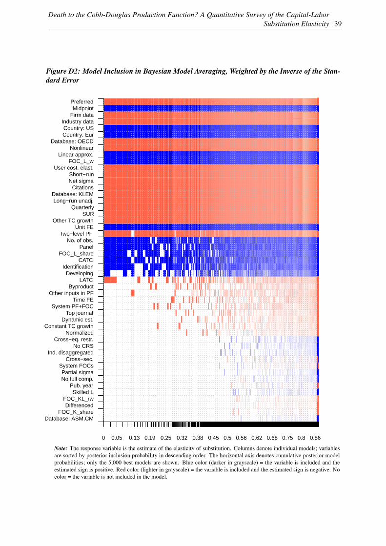
Death to the Cobb-Douglas Production Function? A Quantitative Survey of the Capital-LaborSubstitution Elasticity 39
Figure D2: Model Inclusion in Bayesian Model Averaging, Weighted by the Inverse of the Stan-dard Error
0 0.05 0.13 0.19 0.25 0.32 0.38 0.45 0.5 0.56 0.62 0.68 0.75 0.8 0.86
PreferredMidpoint
Firm dataIndustry data Country: US Country: Eur
Database: OECD Nonlinear
Linear approx. FOC_L_w
User cost. elast. Short−runNet sigma
Citations Database: KLEM Long−run unadj.
Quarterly SUR
Other TC growth Unit FE
Two−level PFNo. of obs.
PanelFOC_L_share
CATC Identification
DevelopingLATC
ByproductOther inputs in PF
Time FESystem PF+FOC
Top journal Dynamic est.
Constant TC growth Normalized
Cross−eq. restr. No CRS
Ind. disaggregated Cross−sec.
System FOCs Partial sigmaNo full comp.
Pub. yearSkilled L
FOC_KL_rw Differenced
FOC_K_share Database: ASM,CM
Note: The response variable is the estimate of the elasticity of substitution. Columns denote individual models; variablesare sorted by posterior inclusion probability in descending order. The horizontal axis denotes cumulative posterior modelprobabilities; only the 5,000 best models are shown. Blue color (darker in grayscale) = the variable is included and theestimated sign is positive. Red color (lighter in grayscale) = the variable is included and the estimated sign is negative. Nocolor = the variable is not included in the model.
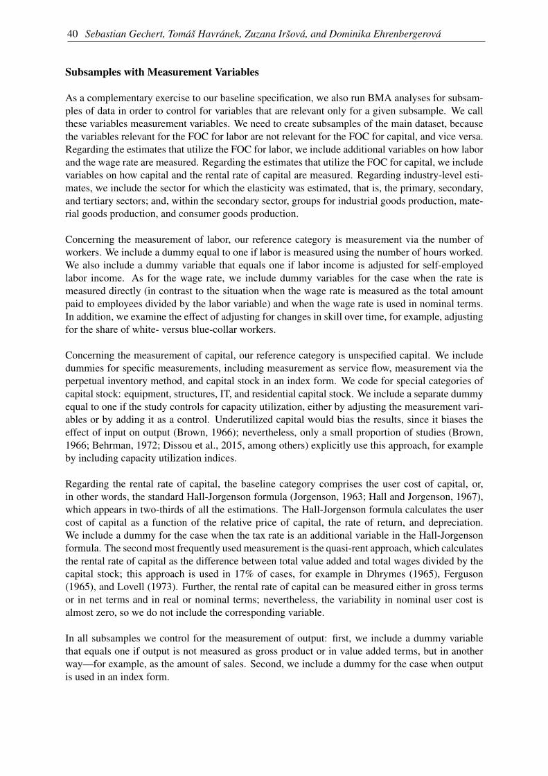
40 Sebastian Gechert, Tomáš Havránek, Zuzana Iršová, and Dominika Ehrenbergerová
Subsamples with Measurement Variables
As a complementary exercise to our baseline specification, we also run BMA analyses for subsam-ples of data in order to control for variables that are relevant only for a given subsample. We callthese variables measurement variables. We need to create subsamples of the main dataset, becausethe variables relevant for the FOC for labor are not relevant for the FOC for capital, and vice versa.Regarding the estimates that utilize the FOC for labor, we include additional variables on how laborand the wage rate are measured. Regarding the estimates that utilize the FOC for capital, we includevariables on how capital and the rental rate of capital are measured. Regarding industry-level esti-mates, we include the sector for which the elasticity was estimated, that is, the primary, secondary,and tertiary sectors; and, within the secondary sector, groups for industrial goods production, mate-rial goods production, and consumer goods production.
Concerning the measurement of labor, our reference category is measurement via the number ofworkers. We include a dummy equal to one if labor is measured using the number of hours worked.We also include a dummy variable that equals one if labor income is adjusted for self-employedlabor income. As for the wage rate, we include dummy variables for the case when the rate ismeasured directly (in contrast to the situation when the wage rate is measured as the total amountpaid to employees divided by the labor variable) and when the wage rate is used in nominal terms.In addition, we examine the effect of adjusting for changes in skill over time, for example, adjustingfor the share of white- versus blue-collar workers.
Concerning the measurement of capital, our reference category is unspecified capital. We includedummies for specific measurements, including measurement as service flow, measurement via theperpetual inventory method, and capital stock in an index form. We code for special categories ofcapital stock: equipment, structures, IT, and residential capital stock. We include a separate dummyequal to one if the study controls for capacity utilization, either by adjusting the measurement vari-ables or by adding it as a control. Underutilized capital would bias the results, since it biases theeffect of input on output (Brown, 1966); nevertheless, only a small proportion of studies (Brown,1966; Behrman, 1972; Dissou et al., 2015, among others) explicitly use this approach, for exampleby including capacity utilization indices.
Regarding the rental rate of capital, the baseline category comprises the user cost of capital, or,in other words, the standard Hall-Jorgenson formula (Jorgenson, 1963; Hall and Jorgenson, 1967),which appears in two-thirds of all the estimations. The Hall-Jorgenson formula calculates the usercost of capital as a function of the relative price of capital, the rate of return, and depreciation.We include a dummy for the case when the tax rate is an additional variable in the Hall-Jorgensonformula. The second most frequently used measurement is the quasi-rent approach, which calculatesthe rental rate of capital as the difference between total value added and total wages divided by thecapital stock; this approach is used in 17% of cases, for example in Dhrymes (1965), Ferguson(1965), and Lovell (1973). Further, the rental rate of capital can be measured either in gross termsor in net terms and in real or nominal terms; nevertheless, the variability in nominal user cost isalmost zero, so we do not include the corresponding variable.
In all subsamples we control for the measurement of output: first, we include a dummy variablethat equals one if output is not measured as gross product or in value added terms, but in anotherway—for example, as the amount of sales. Second, we include a dummy for the case when outputis used in an index form.
Death to the Cobb-Douglas Production Function? A Quantitative Survey of the Capital-LaborSubstitution Elasticity 41
How does the addition of these variables affect our results? First, we include labor-specific vari-ables, which capture how labor and the wage rate are measured, and run BMA on the subsampleof data estimating the FOC for labor. The subsample covers less than half of the original dataset;the results are displayed in Figure D3. Only two of the newly included measurement variables areimportant for the explanation of the heterogeneity in the reported elasticities: direct measurementof the wage rate and measurement of labor as total labor force. The main drivers of heterogeneityremain the same, while the total explanatory power of the analysis increases only marginally.
Concerning capital-related variables, we find that the type of capital under examination represents animportant driver of the differences in results (Figure D4). IT capital and equipment capital are moresubstitutable with labor than other types of capital, such as buildings. When capital is measured asservice flow, the estimates typically yield a larger elasticity of substitution. It also matters how therental rate of capital, r, is computed, specifically whether the Hall-Jorgenson formula is used—wefind that it yields smaller elasticities than do other approaches. The best-practice estimate derivedfrom both subsamples and conditional on plugging in mean values for measurement variables wouldagain equal 0.3, very far from the Cobb-Douglas assumption.
Finally, for the subsample of disaggregated elasticities we run the baseline BMA enriched withindustry-relevant variables in Figure D5. We do not find any significant determinants that wouldsuggest that the elasticity of capital-labor substitution differs systematically across sectors or indus-try groups (production of materials, production of industrial goods, production of consumer goods,and production of services). Given the number of variables in our analysis, it is infeasible to addmore industry-specific variables, since that would create troubles with collinearity.
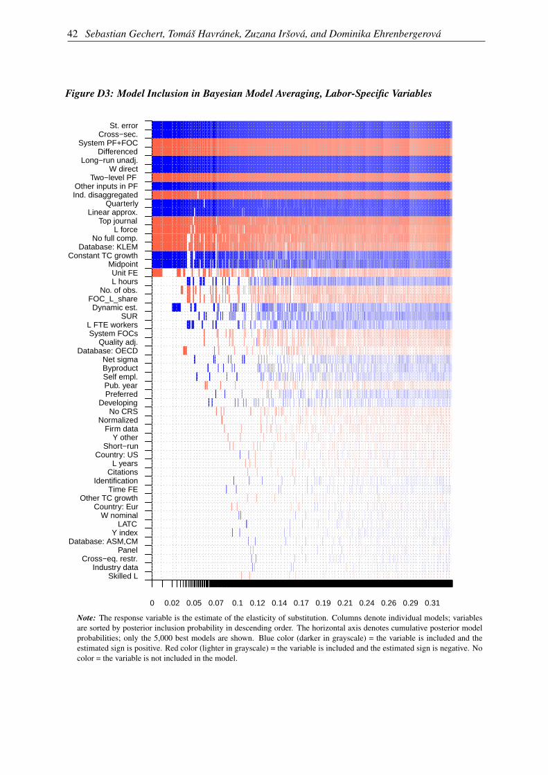
42 Sebastian Gechert, Tomáš Havránek, Zuzana Iršová, and Dominika Ehrenbergerová
Figure D3: Model Inclusion in Bayesian Model Averaging, Labor-Specific Variables
0 0.02 0.05 0.07 0.1 0.12 0.14 0.17 0.19 0.21 0.24 0.26 0.29 0.31
St. errorCross−sec.
System PF+FOC Differenced
Long−run unadj. W direct
Two−level PF Other inputs in PF Ind. disaggregated
QuarterlyLinear approx.
Top journalL force
No full comp. Database: KLEM
Constant TC growth MidpointUnit FEL hours
No. of obs.FOC_L_share Dynamic est.
SURL FTE workers System FOCs
Quality adj. Database: OECD
Net sigma ByproductSelf empl.Pub. year Preferred
DevelopingNo CRS
NormalizedFirm data
Y otherShort−run
Country: USL years
Citations Identification
Time FEOther TC growth
Country: EurW nominal
LATCY index
Database: ASM,CM Panel
Cross−eq. restr. Industry data
Skilled L
Note: The response variable is the estimate of the elasticity of substitution. Columns denote individual models; variablesare sorted by posterior inclusion probability in descending order. The horizontal axis denotes cumulative posterior modelprobabilities; only the 5,000 best models are shown. Blue color (darker in grayscale) = the variable is included and theestimated sign is positive. Red color (lighter in grayscale) = the variable is included and the estimated sign is negative. Nocolor = the variable is not included in the model.

Death to the Cobb-Douglas Production Function? A Quantitative Survey of the Capital-LaborSubstitution Elasticity 43
Figure D4: Model Inclusion in Bayesian Model Averaging, Capital-Specific Variables
0 0.02 0.04 0.07 0.09 0.12 0.14 0.17 0.19 0.22 0.24 0.27 0.29 0.31 0.34
St. errorCountry: US
Long−run unadj. K: IT
K: equipmentNet sigma
Capacity adj.Top journalK: services
K: perpetualY: other
Database: OECD Unit FEr: quasi
Firm dataShort−run
Two−level PF SUR
Developingr: nominal
System PF+FOC r: UCC
Industry data Cross−eq. restr.
r: UCC tax Byproduct
FOC_K_share Skilled L
Other inputs in PF K: residential
Quarterly Dynamic est.
Preferred Database: KLEM
Normalizedr: other
Linear approx. System FOCs
Constant TC growth Country: Eur
CitationsUser cost. elast.
Pub. yearCATC
Identification Differenced
PanelK: index
No. of obs. Midpoint
Cross−sec. Database: ASM,CM
K: structuresNo full comp.
Ind. disaggregated Time FENo CRS
Note: The response variable is the estimate of the elasticity of substitution. Columns denote individual models; variablesare sorted by posterior inclusion probability in descending order. The horizontal axis denotes cumulative posterior modelprobabilities; only the 5,000 best models are shown. Blue color (darker in grayscale) = the variable is included and theestimated sign is positive. Red color (lighter in grayscale) = the variable is included and the estimated sign is negative. Nocolor = the variable is not included in the model.
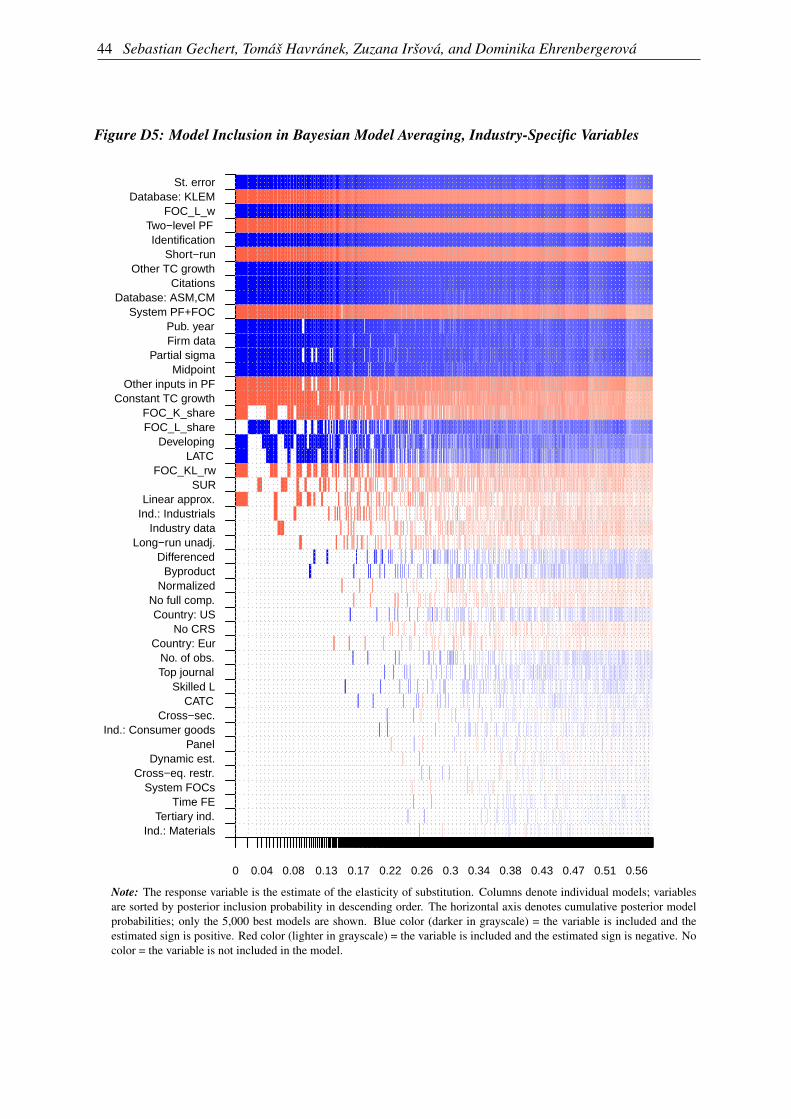
44 Sebastian Gechert, Tomáš Havránek, Zuzana Iršová, and Dominika Ehrenbergerová
Figure D5: Model Inclusion in Bayesian Model Averaging, Industry-Specific Variables
0 0.04 0.08 0.13 0.17 0.22 0.26 0.3 0.34 0.38 0.43 0.47 0.51 0.56
St. errorDatabase: KLEM
FOC_L_wTwo−level PF Identification
Short−runOther TC growth
CitationsDatabase: ASM,CM
System PF+FOC Pub. yearFirm data
Partial sigma Midpoint
Other inputs in PF Constant TC growth
FOC_K_share FOC_L_share
DevelopingLATC
FOC_KL_rw SUR
Linear approx.Ind.: Industrials
Industry dataLong−run unadj.
Differenced Byproduct
NormalizedNo full comp. Country: US
No CRSCountry: Eur
No. of obs.Top journal
Skilled LCATC
Cross−sec.Ind.: Consumer goods
PanelDynamic est.
Cross−eq. restr. System FOCs
Time FETertiary ind.
Ind.: Materials
Note: The response variable is the estimate of the elasticity of substitution. Columns denote individual models; variablesare sorted by posterior inclusion probability in descending order. The horizontal axis denotes cumulative posterior modelprobabilities; only the 5,000 best models are shown. Blue color (darker in grayscale) = the variable is included and theestimated sign is positive. Red color (lighter in grayscale) = the variable is included and the estimated sign is negative. Nocolor = the variable is not included in the model.

Death to the Cobb-Douglas Production Function? A Quantitative Survey of the Capital-LaborSubstitution Elasticity 45
Appendix E: Studies Included in the Dataset
ABED, G. T. (1975): “Labour Absorption inIndustry: An Analysis with Reference toEgypt.” Oxford Economic Papers, 27(3):400–425.
AKAY, G. H. AND C. DOGAN (2013): “TheEffect of Labor Supply Changes on Out-put: Empirical Evidence from US Indus-tries.” Journal of Productivity Analysis,39(2):123–130.
ANTRAS, P. (2004): “Is the US Aggregate Pro-duction Function Cobb-Douglas? NewEstimates of the Elasticity of Substitu-tion.” Contributions in Macroeconomics,4(1):1–36.
APOSTOLAKIS, B. E. (1984): “ATranslogarithmic Cost Function Ap-proach: Greece, 1953–1977.” EmpiricalEconomics, 9(4):247–262.
ARROW, K. J., H. B. CHENERY, B. S. MIN-HAS, AND R. M. SOLOW (1961):“Capital-Labor Substitution and Eco-nomic Efficiency.” Review of Economicsand Statistics, 43(3):225–250.
ARTUS, J. R. (1984): “The DisequilibriumReal Wage Rate Hypothesis: An Empiri-cal Evaluation.” Staff Papers, 31(2):249–302.
ASHER, E. (1972): “Industrial Efficiencyand Biased Technical Change in Ameri-can and British Manufacturing: The Caseof Textiles in the Nineteenth Century.”Journal of Economic History, 32(2):431–442.
BALISTRERI, E. J., C. A. MCDANIEL, AND
E. V. WONG (2003): “An Esti-mation of US Industry-Level Capital–Labor Substitution Elasticities: Supportfor Cobb–Douglas.” North AmericanJournal of Economics and Finance, 14(3):343–356.
BARTELSMAN, E. J. AND R. M. BEETSMA
(2003): “Why Pay More? CorporateTax Avoidance through Transfer Pricing
in OECD Countries.” Journal of PublicEconomics, 87(9-10):2225–2252.
BEHRMAN, J. (1982): Country and SectoralVariations in Manufacturing Elasticitiesof Substitution between Capital and La-bor. In Trade and Employment in De-veloping Countries, Volume 2: FactorSupply and Substitution, pages 159–192.University of Chicago.
BEHRMAN, J. R. (1972): “Sectoral Elastici-ties of Substitution between Capital andLabor in a Developing Economy: TimesSeries Analysis in the Case of PostwarChile.” Econometrica, 40(2):311–326.
BENTOLILA, S. AND G. SAINT-PAUL (2003):“Explaining Movements in the LaborShare.” Contributions in Macroeco-nomics, 3(1):1–33.
BERNDT, E. R. (1976): “Reconciling Alterna-tive Estimates of the Elasticity of Substi-tution.” Review of Economics and Statis-tics, 58(1):59–68.
BERTHOLD, N., R. FEHN, AND E. THODE
(2002): “Falling Labor Share and Ris-ing Unemployment: Long–Run Conse-quences of Institutional Shocks?.” Ger-man Economic Review, 3(4):431–459.
BINSWANGER, H. P. (1974): “A Cost FunctionApproach to the Measurement of Elastic-ities of Factor Demand and Elasticities ofSubstitution.” American Journal of Agri-cultural Economics, 56(2):377–386.
BLANCHARD, O. J. (1997): “The MediumRun.” Brookings Papers on EconomicActivity, 1997(2):89–141.
BODKIN, R. G. AND L. R. KLEIN (1967):“Nonlinear Estimation of Aggregate Pro-duction Functions.” Review of Economicand Statistics, 49(1):28–44.
BROWN, M. (1966): “A Measure of the Changein Relative Exploitation of Capital andLabor.” Review of Economics and Statis-tics, 48(2):182–192.
BROWN, M. AND J. S. DE CANI (1963):“Technological Change and the Distribu-
46 Sebastian Gechert, Tomáš Havránek, Zuzana Iršová, and Dominika Ehrenbergerová
tion of Income.” International EconomicReview, 4(3):289–309.
BROX, J. A. AND C. A. FADER (2005):“Infrastructure Investment and CanadianManufacturing Productivity.” AppliedEconomics, 37(11):1247–1256.
BRUNO, M. AND J. SACHS (1982): “InputPrice Shocks and the Slowdown in Eco-nomic Growth: The Case of UK Manu-facturing.” Review of Economic Studies,49(5):679–705.
CABALLERO, R. J. (1994): “Small Sample Biasand Adjustment Costs.” Review of Eco-nomics and Statistics, 76(1):52–58.
CHETTY, V. K. AND U. SANKAR (1969):“Bayesian Estimation of the CES Pro-duction Function.” Review of EconomicStudies, 36(3):289–294.
CHIRINKO, R. S. AND D. MALLICK (2017):“The Substitution Elasticity, FactorShares, and the Low-Frequency PanelModel.” American Economic Journal:Macroeconomics, 9(4):225–53.
CHIRINKO, R. S., S. M. FAZZARI, AND A. P.MEYER (1999): “How Responsive IsBusiness Capital Formation to its UserCost? An Exploration with Micro Data.”Journal of Public Economics, 74(1):53–80.
CHIRINKO, R. S., S. M. FAZZARI, AND A. P.MEYER (2011): “A New Approach toEstimating Production Function Parame-ters: The Elusive Capital–Labor Substi-tution Elasticity.” Journal of Business &Economic Statistics, 29(4):587–594.
CHWELOS, P., R. RAMIREZ, K. L. KRAEMER,AND N. P. MELVILLE (2010): “DoesTechnological Progress Alter the Natureof Information Technology as a Produc-tion Input? New Evidence and New Re-sults.” Information Systems Research, 21(2):392–408.
CLARK, P. K. AND D. E. SICHEL (1993): “TaxIncentives and Equipment Investment.”Brookings Papers on Economic Activity,1993(1):317–347.
CLARO, S. (2003): “A Cross-Country Estima-
tion of the Elasticity of Substitution be-tween Labor and Capital in Manufactur-ing Industries.” Cuadernos de economía,40(120):239–257.
CUMMINS, J. G. AND K. A. HASSETT (1992):“The Effects of Taxation on Investment:New Evidence from Firm Level PanelData.” National Tax Journal, 45(3):243–251.
CUMMINS, J. G., K. A. HASSETT, R. G. HUB-BARD, R. E. HALL, AND R. J. CA-BALLERO (1994): “A Reconsiderationof Investment Behavior Using Tax Re-forms as Natural Experiments.” Brook-ings Papers on Economic Activity, 1994(2):1–74.
DANIELS, M. R. (1969): “Differences in Ef-ficiency among Industries in DevelopingCountries.” American Economic Review,59(1):159–171.
DAVID, P. A. AND T. VAN DE KLUNDERT
(1965): “Biased Efficiency Growth andCapital-Labor Substitution in the US,1899-1960.” American Economic Re-view, 55(3):357–394.
DHRYMES, P. J. (1965): “Some Extensionsand Tests for the CES Class of Produc-tion Functions.” Review of Economicsand Statistics, 47(4):357–366.
DISSOU, Y. AND R. GHAZAL (2010): “En-ergy Substitutability in Canadian Man-ufacturing Econometric Estimation withBootstrap Confidence Intervals.” EnergyJournal, 31(1):121–148.
DISSOU, Y., L. KARNIZOVA, AND Q. SUN
(2015): “Industry-Level EconometricEstimates of Energy-Capital-Labor Sub-stitution with a Nested CES ProductionFunction.” Atlantic Economic Journal,43(1):107–121.
DONGES, J. B. (1972): “Returns to Scale andFactor Substitutability in the Spanish In-dustry.” Review of World Economics, 108(4):597–608.
DUFFY, J. AND C. PAPAGEORGIOU (2000):“A Cross-Country Empirical Investiga-tion of the Aggregate Production Func-tion Specification.” Journal of Economic

Death to the Cobb-Douglas Production Function? A Quantitative Survey of the Capital-LaborSubstitution Elasticity 47
Growth, 5(1):87–120.DWENGER, N. (2014): “User Cost Elasticity of
Capital Revisited.” Economica, 81(321):161–186.
EASTERLY, W. AND S. FISCHER (1995): “TheSoviet Economic Decline.” World BankEconomic Review, 9(3):341–371.
EISNER, R. (1967): Capital and Labor in Pro-duction: Some Direct Estimates. In TheTheory and Empirical Analysis of Pro-duction, pages 431–475. NBER.
EISNER, R. (1969): “Tax Policy and Invest-ment Behavior: Comment.” AmericanEconomic Review, 59(3):379–388.
EISNER, R. AND M. I. NADIRI (1968): “Invest-ment Behavior and Neo-Classical The-ory.” Review of Economics and Statis-tics, 50(3):369–382.
ELBERS, C., J. W. GUNNING, AND B. KINSEY
(2007): “Growth and Risk: Methodol-ogy and Micro Evidence.” World BankEconomic Review, 21(1):1–20.
ELLIS, C. AND S. PRICE (2004): “UK BusinessInvestment and the User Cost of Capi-tal.” Manchester School, 72:72–93.
FELDSTEIN, M. S. (1967): “Specification ofthe Labour Input in the Aggregate Pro-duction Function.” Review of EconomicStudies, 34(4):375–386.
FELDSTEIN, M. S. AND J. S. FLEMMING
(1971): “Tax Policy, Corporate Savingand Investment Behaviour in Britain.”Review of Economic Studies, 38(4):415–434.
FELIPE, J. AND J. MCCOMBIE (2009): “AreEstimates of Labour Demand FunctionsMere Statistical Artefacts?.” Interna-tional Review of Applied Economics, 23(2):147–168.
FERGUSON, C. E. (1965): “Time-SeriesProduction Functions and TechnologicalProgress in American Manufacturing In-dustry.” Journal of Political Economy, 73(2):135–147.
FISHELSON, G. (1979): “Elasticity of FactorSubstitution in Cross-Section ProductionFunctions.” Review of Economics and
Statistics, 61(3):432–436.FITCHETT, D. A. (1976): “Capital-Labor Sub-
stitution in the Manufacturing Sector ofPanama.” Economic Development andCultural Change, 24(3):577–592.
FUCHS, V. R. (1963): “Capital-Labor Substitu-tion: A Note.” Review of Economics andStatistics, 45(4):436–438.
GRILICHES, Z. (1964): “Research Ex-penditures, Education, and the Aggre-gate Agricultural Production Function.”American Economic Review, 54(6):961–974.
GRILICHES, Z. (1967): Production Func-tions in Manufacturing: Some Prelimi-nary Results. In The Theory and Empir-ical Analysis of Production, pages 275–340. NBER.
HERRENDORF, B., C. HERRINGTON, AND
A. VALENTINYI (2015): “SectoralTechnology and Structural Transforma-tion.” American Economic Journal:Macroeconomics, 7(4):104–33.
HIJZEN, A. AND P. SWAIM (2010): “Off-shoring, Labour Market Institutions andthe Elasticity of Labour Demand.” Eu-ropean Economic Review, 54(8):1016–1034.
HOSSAIN, S. I. (1987): “Allocative and Tech-nical Efficiency: A Study of Rural En-terprises in Bangladesh.” DevelopingEconomies, 25(1):56–72.
HUMPHREY, D. B. AND J. R. MORONEY
(1975): “Substitution among Capital,Labor, and Natural Resource Products inAmerican Manufacturing.” Journal ofPolitical Economy, 83(1):57–82.
IQBAL, M. (1986): “Substitution of Labour,Capital and Energy in the Manufactur-ing Sector of Pakistan.” Empirical Eco-nomics, 11(2):81–95.
JALAVA, J., M. POHJOLA, A. RIPATTI, AND
J. VILMUNEN (2006): “Biased Tech-nical Change and Capital-Labour Substi-tution in Finland, 1902-2003.” Topics inMacroeconomics, 6(1):1–20.
JONES, D. C. AND D. K. BACKUS (1977):
48 Sebastian Gechert, Tomáš Havránek, Zuzana Iršová, and Dominika Ehrenbergerová
“British Producer Cooperatives in theFootware Industry: An Empirical Eval-uation of the Theory of Financing.” Eco-nomic Journal, 87(347):488–510.
JUDZIK, D. AND H. SALA (2015): “The Deter-minants of Capital Intensity in Japan andthe US.” Journal of the Japanese and In-ternational Economies, 35:78–98.
JUSELIUS, M. (2008): “Long-Run Relation-ships between Labor and Capital: Indi-rect Evidence on the Elasticity of Substi-tution.” Journal of Macroeconomics, 30(2):739–756.
KALT, J. P. (1978): “Technological Change andFactor Substitution in the United States:1929-1967.” International Economic Re-view, 19(3):761–775.
KARABARBOUNIS, L. AND B. NEIMAN
(2013): “The Global Decline of theLabor Share.” Quarterly Journal ofEconomics, 129(1):61–103.
KILPONEN, J. AND M. VIREN (2010): “WhyDo Growth Rates Differ? Evidence fromCross-Country Data on Private SectorProduction.” Empirica, 37(3):311–328.
KISLEV, Y. AND W. PETERSON (1982):“Prices, Technology, and Farm Size.”Journal of Political Economy, 90(3):578–595.
KLUMP, R., P. MCADAM, AND A. WILLMAN
(2007): “Factor Substitution and Factor-Augmenting Technical Progress in theUnited States: A Normalized Supply-Side System Approach.” Review of Eco-nomics and Statistics, 89(1):183–192.
KLUMP, R., P. MCADAM, AND A. WILL-MAN (2008): “Unwrapping Some EuroArea Growth Puzzles: Factor Substitu-tion, Productivity and Unemployment.”Journal of Macroeconomics, 30(2):645–666.
KMENTA, J. (1967): “On Estimation ofthe CES Production Function.” Interna-tional Economic Review, 8(2):180–189.
KRUSELL, P., L. E. OHANIAN, J.-V. ROOS-RULL, AND G. L. VIOLANTE (2000):“Capital-Skill Complementarity and In-
equality: A Macroeconomic Analysis.”Econometrica, 68(5):1029–1053.
LEE, M. AND M. TCHA (2004): “The Colorof Money: The Effects of Foreign Di-rect Investment on Economic Growth inTransition Economies.” Review of WorldEconomics, 140(2):211–229.
LEÓN-LEDESMA, M. A., P. MCADAM, AND
A. WILLMAN (2015): “Produc-tion Technology Estimates and BalancedGrowth.” Oxford Bulletin of Economicsand Statistics, 77(1):40–65.
LEUNG, D. AND T. YUEN (2010): “Do Ex-change Rates Affect the Capital–LabourRatio? Panel Evidence from CanadianManufacturing Industries.” Applied Eco-nomics, 42(20):2519–2535.
LIANOS, T. P. (1971): “The Relative Shareof Labor in United States Agriculture,1949–1968.” American Journal of Agri-cultural Economics, 53(3):411–422.
LIANOS, T. P. (1975): “Capital-Labor Substitu-tion in a Developing Country: The Caseof Greece.” European Economic Review,6(2):129–141.
LIN, W. T. AND B. B. SHAO (2006): “TheBusiness Value of Information Technol-ogy and Inputs Substitution: The Pro-ductivity Paradox Revisited.” DecisionSupport Systems, 42(2):493–507.
LOVELL, C. K. (1973): “Estimation and Pre-diction with CES and VES ProductionFunctions.” International Economic Re-view, 14(3):676–692.
LOVELL, C. K. (1973): “CES and VES Produc-tion Functions in a Cross-Section Con-text.” Journal of Political Economy, 81(3):705–720.
LUOMA, A. AND J. LUOTO (2010): “TheAggregate Production Function of theFinnish Economy in the Twentieth Cen-tury.” Southern Economic Journal, 76(3):723–737.
MALLICK, D. (2012): “The Role of the Elastic-ity of Substitution in Economic Growth:A Cross-Country Investigation.” LabourEconomics, 19(5):682–694.
Death to the Cobb-Douglas Production Function? A Quantitative Survey of the Capital-LaborSubstitution Elasticity 49
MARTIN, S. A., R. MCHUGH, AND S. R.JOHNSON (1993): “The Influence ofLocation on Productivity: Manufactur-ing Technology in Rural and Urban Ar-eas.” Growth and Change, 24(4):459–486.
MASANJALA, W. H. AND C. PAPAGEORGIOU
(2004): “The Solow Model with CESTechnology: Nonlinearities and Param-eter Heterogeneity.” Journal of AppliedEconometrics, 19(2):171–201.
MCADAM, P. AND A. WILLMAN (2004): “Pro-duction, Supply and Factor Shares: AnApplication to Estimating German Long-Run Supply.” Economic Modelling, 21(2):191–215.
MCCALLUM, J. (1985): “Wage Gaps, FactorShares and Real Wages.” ScandinavianJournal of Economics, 87(2):436–459.
MCKINNON, R. I. (1962): “Wages, CapitalCosts, and Employment in Manufactur-ing: A Model Applied to 1947-58 USData.” Econometrica, 30(3):501–521.
MCLEAN-MEYINSSE, P. E. AND A. A. OKU-NADE (1988): “Factor Demands ofLouisiana Rice Producers: An Econo-metric Investigation.” Journal of Agri-cultural and Applied Economics, 20(2):127–136.
MELLER, P. (1975): Production Functionsfor Industrial Establishments of Differ-ent Sizes: The Chilean Case. In An-nals of Economic and Social Measure-ment, Volume 4, number 4, pages 595–634. NBER.
MINASIAN, J. R. (1961): “Elasticities of Sub-stitution and Constant-Output DemandCurves for Labor.” Journal of PoliticalEconomy, 69(3):261–270.
MOHABBAT, K. A. AND A. J. DALAI (1983):“Factor Substitution and Import Demandfor South Korea: A Translog Analy-sis.” Review of World Economics, 119(4):709–723.
MOHABBAT, K. A., A. DALAL, AND
M. WILLIAMS (1984): “ImportDemand for India: A Translog CostFunction Approach.” Economic De-
velopment and Cultural Change, 32(3):593–605.
MORONEY, J. R. (1966): “Time-Series Elas-ticities of Substitution and Labor’s Sharein US Manufacturing: The Postwar Pe-riod.” Southern Economic Journal, 32(4):474.
MORONEY, J. R. (1970): “Identificationand Specification Analysis of AlternativeEquations for Estimating the Elasticity ofSubstitution.” Southern Economic Jour-nal, 36(3):287–299.
MORONEY, J. R. AND B. T. ALLEN (1969):“Monopoly Power and the RelativeShare of Labor.” ILR Review, 22(2):167–178.
MORONEY, J. R. AND A. L. TOEVS (1977):“Factor Costs and Factor Use: An Anal-ysis of Labor, Capital, and Natural Re-source Inputs.” Southern EconomicJournal, 44(2):222–239.
NADIRI, M. I. (1968): “The Effects of Rela-tive Prices and Capacity on the Demandfor Labour in the US Manufacturing Sec-tor.” Review of Economic Studies, 35(3):273–288.
PANIK, M. J. (1976): “Factor Learning andBiased Factor-Efficiency Growth in theUnited States, 1929-1966.” InternationalEconomic Review, 17(3):733–739.
PARKS, R. W. (1971): “Price Responsivenessof Factor Utilization in Swedish Manu-facturing, 1870-1950.” Review of Eco-nomics and Statistics, 53(2):129–139.
POLLAK, R. A., R. C. SICKLES, AND T. J.WALES (1984): “The CES-Translog:Specification and Estimation of a NewCost Function.” Review of Economicsand Statistics, 66(4):602–607.
RAURICH, X., H. SALA, AND V. SOROLLA
(2012): “Factor Shares, the PriceMarkup, and the Elasticity of Substitu-tion between Capital and Labor.” Jour-nal of Macroeconomics, 34(1):181–198.
ROSKAMP, K. W. (1977): “Labor Productivityand the Elasticity of Factor Substitutionin West German Industries 1950-1960.”

50 Sebastian Gechert, Tomáš Havránek, Zuzana Iršová, and Dominika Ehrenbergerová
Review of Economics and Statistics, 59(3):366–371.
SAHOTA, G. S. (1966): “The Sources ofMeasured Productivity Growth: UnitedStates Fertilizer Mineral Industries,1936-1960.” Review of Economics andStatistics, 48(2):193–204.
SALVANES, K. G. (1989): “The Structureof the Norwegian Fish Farming Industry:An Empirical Analysis of Economiesof Scale and Substitution Possibilities.”Marine Resource Economics, 6(4):349–373.
SANKAR, U. (1972): “Investment Behaviorin the US Electric Utility Industry, 1949-1968.” Bell Journal of Economics, 3(2):645–664.
SAPIR, A. (1980): “Economic Growth and Fac-tor Substitution: What Happened to theYugoslav Miracle?.” Economic Journal,90(358):294–313.
SATO, K. (1977): “A note on Factor Substi-tution and Efficiency.” Review of Eco-nomics and Statistics, 59(3):360–366.
SATO, R. AND R. F. HOFFMAN (1968): “Pro-duction Functions with Variable Elastic-ity of Factor Substitution: Some Analy-sis and Testing.” Review of Economicsand Statistics, 50(4):453–460.
SAXONHOUSE, G. (1977): “Productiv-ity Change and Labor Absorption inJapanese Cotton Spinning 1891–1935.”Quarterly Journal of Economics, 91(2):195–219.
SCHALLER, H. (2006): “Estimating the Long-Run User Cost Elasticity.” Journal ofMonetary Economics, 53(4):725–736.
SCHMITZ, M. (1981): “The Elasticity ofSubstitution in 19th-Century Manufac-turing.” Explorations in Economic His-tory, 18(3):290.
SEMIENIUK, G. (2017): “Piketty’s Elasticityof Substitution: A Critique.” Review ofPolitical Economy, 29(1):64–79.
SHAHE EMRAN, M., F. SHILPI, AND M. I.ALAM (2007): “Economic Liberal-ization and Price Response of Aggre-gate Private Investment: Time Series Ev-idence from India.” Canadian Journal ofEconomics, 40(3):914–934.
SMITH, J. (2008): “That Elusive Elasticityand the Ubiquitous Bias: Is Panel Data aPanacea?.” Journal of Macroeconomics,30(2):760–779.
SOLOW, R. (1964): Capital, Labor, and In-come in Manufacturing. In The Behav-ior of Income Shares: Selected Theoret-ical and Empirical Issues, pages 101–142. Princeton University Press.
TEVLIN, S. AND K. WHELAN (2003): “Ex-plaining the Investment Boom of the1990s.” Journal of Money, Credit andBanking, 35(1):1–22.
TSANG, H. H. AND J. J. PERSKY (1975): “Onthe Empirical Content of CES Produc-tion Functions.” Economic Record, 51(4):539–548.
VAN DER WERF, E. (2008): “Production Func-tions for Climate Policy Modeling: AnEmpirical Analysis.” Energy Economics,30(6):2964–2979.
WEITZMAN, M. L. (1970): “Soviet PostwarEconomic Growth and Capital-LaborSubstitution.” American Economic Re-view, 60(4):676–692.
WILLIAMS, M. AND P. S. LAUMAS (1984):“Economies of Scale for Various Typesof Manufacturing Production Technolo-gies in an Underdeveloped Economy.”Economic Development and CulturalChange, 32(2):401–412.
YOUNG, A. T. (2013): “US Elasticities ofSubstitution and Factor Augmentation atthe Industry Level.” Macroeconomic Dy-namics, 17(4):861–897.
ZAREMBKA, P. (1970): “On the Empirical Rel-evance of the CES Production Function.”Review of Economics and Statistics, 52(1):47–53.

CNB WORKING PAPER SERIES (SINCE 2018)
8/2019 Sebastian Gechert
Tomáš Havránek
Zuzana Iršová
Dominika
Ehrenbergerová
Death to the Cobb-Douglas production function? A quantitative
survey of the capital-labor substitution elasticity
7/2019 Alexis Derviz Coexistence of physical and crypto assets in a stochastic
endogenous growth model
6/2019 Dominika
Ehrenbergerová
Simona Malovaná
Introducing macro-financial variables into semi-structural model
5/2019 Martin Hodula Monetary policy and shadow banking: Trapped between a rock
and a hard place
4/2019 Simona Malovaná
Žaneta Tesařová
Banks’ credit losses and provisioning over the business cycle:
Implications for IFRS 9
3/2019 Aleš Bulíř
Jan Vlček
Monetary policy is not always systematic and data-driven:
Evidence from the yield curve
2/2019 Dominika Kolcunová
Simona Malovaná
The effect of higher capital requirements on bank lending: The
capital surplus matters
1/2019 Jaromír Baxa
Tomáš Šestořád
The Czech exchange rate floor: Depreciation without inflation?
19/2018 Jan Brůha
Jaromír Tonner
Independent monetary policy versus common currency: The
macroeconomic analysis for the Czech Republic through lens of an
applied DSGE model
18/2018 Tomáš Adam
Filip Novotný
Assessing the external demand of the Czech economy: Nowcasting
foreign GDP using bridge equations
17/2018 Kamil Galuščák
Jan Šolc
Pawel Strzelecki
Labour market flows over the business cycle: The role of the
participation margin
16/2018 Martin Hodula Off the radar: Exploring the rise of shadow banking in the EU
15/2018 Lukáš Pfeifer
Martin Hodula
Libor Holub
Zdeněk Pikhart
The leverage ratio and its impact on capital regulation
14/2018 Martin Gürtler What influences private investment? The case of the Czech
Republic
13/2018 Václav Hausenblas
Jitka Lešanovská
How do large banking groups manage the efficiency of their
subsidiaries? Evidence from CEE
12/2018 Simona Malovaná The pro-cyclicality of risk weights for credit exposures in the
Czech Republic
11/2018 Tibor Hlédik
Karel Musil
Jakub Ryšánek
Jaromír Tonner
A macroeconomic forecasting model of the fixed exchange rate
regime for the oil-rich Kazakh economy
10/2018 Michal Franta
Tomáš Holub
Branislav Saxa
Balance sheet implications of the Czech National Bank’s exchange
rate commitment
9/2018 Dominika Kolcunová
Tomáš Havránek
Estimating the effective lower bound on the Czech National Bank’s
policy rate

8/2018 Volha Audzei
Sergey Slobodyan
Sparse restricted perception equilibrium
7/2018 Tibor Hlédik
Jan Vlček
Quantifying the natural rate of interest in a small open economy –
The Czech case
6/2018 Václav Brož
Michal Hlaváček
What drives distributional dynamics of client interest rates on
consumer loans in the Czech Republic? A bank-level analysis
5/2018 Lukáš Pfeifer
Martin Hodula
Profit-to-provisioning approach for setting the countercyclical
capital buffer: The Czech example
4/2018 Ivan Sutóris Asset prices in a production economy with long run and
idiosyncratic risk
3/2018 Michal Franta The likelihood of effective lower bound events
2/2018 Soňa Benecká
Ludmila Fadejeva
Martin Feldkircher
Spillovers from euro area monetary policy: A focus on emerging
Europe
1/2018 Jan Babecký
Clémence Berson
Ludmila Fadejeva
Ana Lamo
Petra Marotzke
Fernando Martins
Pawel Strzelecki
Non-base wage components as a source of wage adaptability to
shocks: Evidence from European firms, 2010-2013
CNB RESEARCH AND POLICY NOTES (SINCE 2018)
2/2019 Jan Filáček
Ivan Sutóris
Inflation targeting flexibility: The CNB’s reaction function under
scrutiny
1/2019 Iveta Polášková
Luboš Komárek
Michal Škoda
The contemporary role of gold in central banks’ balance sheets
1/2018 Mojmír Hampl
Tomáš Havránek
Central bank financial strength and inflation: A meta-analysis
CNB ECONOMIC RESEARCH BULLETIN (SINCE 2018)
November 2018 Interest rates
May 2018 Risk-sensitive capital regulation


Czech National Bank
Economic Research Division Na Příkopě 28, 115 03 Praha 1
Czech Republic
phone: +420 2 244 12 321
fax: +420 2 244 12 329
http://www.cnb.cz
e-mail: [email protected]
ISSN 1803-7070