working paper series recessions that occur in tandem with banking crises. thus, the expansionary and...
TRANSCRIPT

Working Paper Series Detrending and financial cycle facts across G7 countries: mind a spurious medium term!
Yves S. Schüler
Disclaimer: This paper should not be reported as representing the views of the European Central Bank (ECB). The views expressed are those of the authors and do not necessarily reflect those of the ECB.
No 2138 / March 2018
Abstract
I show that the detrending of financial variables with the Hodrick and Prescott (1981, 1997) (HP)and band-pass filters leads to spurious cycles. I find that distortions become especially severe whenconsidering medium-term cycles, i.e., cycles that exceed the duration of regular business cycles. Inparticular, these medium-term filters amplify the variances of cycles of duration around 20 to 30years up to a factor of 204, completely cancelling out shorter-term fluctuations. This is importantbecause it is common practice, and recommended under Basel III, to extract medium-term cyclesusing such filters; e.g., the HP filter with a smoothing parameter of 400,000. In addition, I find thatfinancial cycle facts, i.e., differing amplitude, duration, and synchronisation of cycles in financialvariables relative to cycles in GDP, are robust. For HP and band-pass filters, differences to GDPbecome marginal due to spurious cycles.
Keywords: Macroprudential policy · Detrending · Spurious cycles · Financial cycles · Credit-to-GDP gap
JEL-Codes: C10 · E32 · E44 · E58 · G01
ECB Working Paper Series No 2138 / March 2018 1
NON-TECHNICAL SUMMARY
The recent global financial crisis has led to a broad consensus that microprudential, monetary, fiscal,
or other policies may not always assure financial stability, indicating the need to adopt macroprudential
policy. Macroprudential policy addresses the time series and cross-sectional dimensions of systemic
risk.1 Within the time series dimension, macroprudential policy aims to limit the build-up and correction
phases of ebullient cycles in financial variables, which are often accompanied by financial recessions,
i.e., recessions that occur in tandem with banking crises. Thus, the expansionary and contractionary
phases, or cycles, of financial variables are at the centre of macroprudential policy-making.
Financial variables, however, are trending; a feature that masks possible cycles. In the business
cycle context, the variables of interest are trending as well. Here, it is common practice to decompose
the trending variables, such as real output, into a secular (or trend) component and a non-trending, i.e.,
stationary, component that potentially shows cyclical behaviour. Researchers and practitioners in the
financial cycle context have taken a similar approach. However, in contrast to research on business
cycles, studies have stressed that financial cycles are of longer duration, i.e. lasting up to 30 years,
where eight years is regarded as the usual maximum duration of a business cycle. Further, Basel III
regulations advise considering medium-term cycles of the credit-to-GDP ratio to guide the rates of
countercyclical capital buffer (CCyB) by mechanically employing a Hodrick and Prescott (1981, 1997)
(HP) filter with a smoothing parameter of 400,000. The extraction of such medium-duration cycles,
however, is non-standard in the business cycle context and, thus, has not been debated by the previous
literature.
The current study fills this gap by providing insights on the effects of different methods of detrending
on financial variables, among others, considering the extraction of medium-term cycles. Further, using
various methods of detrending, I revisit the question of whether cycles in financial variables are indeed
marked by different characteristics than business cycles. Such evidence can serve as an important
argument for a complementary role of macroprudential policy to other macroeconomic policies that
mainly target the business cycle. Put differently, robust differences would substantiate the argument
that, for example, monetary policy may not be able to efficiently stabilise both the business and financial
cycle.
Findings suggest that the HP and the Baxter and King (1999) (BK) filters induce artificial boom-bust
phases, i.e., spurious cycles, into financial but also business cycle variables. The negative consequences
of spurious cycles are particularly stark when extracting medium-term cycles, for example, using the
HP filter with a smoothing parameter of 400,000. These results also hold for band-pass filters in general,
e.g., the Christiano and Fitzgerald (2003) filter. At a quarterly sampling frequency, extracting medium-
term cycles with the HP or with band-pass filters strongly emphasises a small frequency range that1Systemic risk can, for example, be defined as “the risk that financial instability becomes so widespread that it impairs the
functioning of a financial system to the point where economic growth and welfare suffer materially” (European Central Bank,2009, p. 134).
ECB Working Paper Series No 2138 / March 2018 2

cancels out other, possibly relevant, fluctuations. I show that this amplification strongly biases inference,
for example, when analysing the synchronisation of cycles across countries. Note that extracting cycles
at business cycle frequencies also distorts by amplifying specific frequencies, but to a much lesser extent
and, hence, leads to a smaller bias in inference.
In spite of evidence on spurious cycles, financial cycle facts, i.e., differing properties of financial
variables relative to GDP, are found to be robust to the method of detrending. Differences only become
marginal when considering the HP and BK filters.
Three main policy conclusions may be drawn from this study. First, caution needs to be exercised
when analysing extracted medium-term cycles, as for instance suggested in Basel III. The strong am-
plification of a small range of cycles cancels shorter-term frequencies that could be potentially relevant,
say, in signalling the build-up of imbalances prior to systemic banking crises or the abrupt risk material-
isation thereafter. Also if the frequency of financial crises increases, build-up phases of imbalances will
not be visible when focussing exclusively on a very specific medium-term frequency range. Hence, there
is a high risk that the recommended credit-to-GDP gap will misguide the setting of the CCyB rate. Sec-
ond, assuming the same HP smoothing parameter or BK frequency window across different countries,
means that relevant country-specific fluctuations are likely to be missed. While the US Basel credit-
to-GDP gap indicates imbalances before the savings and loan crisis and the global financial crisis, the
emphasis of such medium-term frequencies does not necessarily imply that Basel credit-to-GDP gaps
signal systemic banking crises for other countries as well – rather the opposite: the strong amplification
of medium-term cycles is prone to miss fluctuations of relevance for other countries. The same argu-
ment also holds for studies researching on business cycles that assume similar detrending specifications
across countries; however, the risk of missing relevant fluctuations is greater when considering medium-
term cycles. Third, differing empirical properties of financial and business cycle variables make a strong
case for macroprudential policy possibly taking a complementary role to other macroeconomic policies
that primarily target business cycles.
ECB Working Paper Series No 2138 / March 2018 3
1 INTRODUCTION
The analysis of the expansionary and contractionary phases, or cycles, in financial variables has become
critical to inform about the build-up of imbalances in the financial sector. One example is the Basel III
credit-to-GDP gap whose cycles guide the setting of countercyclical capital buffers (CCyBs), as the
different phases are claimed to inform about excess aggregate credit growth.2 Here, the identification
of cycles relies on the detrending of the credit-to-GDP ratio with a Hodrick and Prescott (1981, 1997)
filter using a smoothing parameter of 400,000 (HP (400000)), where 1,600 (HP (1600)) is the commonly
employed parameter, for instance, when detrending business cycle indicators. The large parameter is
motivated by results that fluctuations exceeding the duration of regular business cycles, or medium-term
cycles, are important for describing the movements in financial variables; for instance, in signalling
financial crises or when compared to business cycle indicators.3 Due to this reason, various detrending
approaches have already been considered for identifying the expansionary and contractionary phases in
financial variables.
The purpose of this paper is to explore the consequences of these different detrending approaches for
the analysis of the expansionary and contractionary phases in financial variables. Such analysis can be
motivated by previous studies in the context of business cycles. On the one hand, research has stressed
that HP and band-pass filters may generate spurious cycles, in which case, for instance, the duration of
expansionary and contractionary phases is strongly determined by a priori chosen parameters (Harvey
and Jaeger (1993); King and Rebelo (1993); Cogley and Nason (1995); A’Hearn and Woitek (2001);
Pederson (2001); Murray (2003); Hamilton (2017)). On the other hand, studies indicate that differ-
ent detrending procedures lead to different business cycles facts (Canova (1998a,b); Burnside (1998)).
Recent studies suggest that cycles in financial variables relative to cycles in GDP differ in amplitude,
duration, and synchronisation (e.g., Claessens, Kose and Terrones (2011, 2012), Aikman et al. (2015),
or Schüler et al. (2015, 2017)). The robustness of these financial cycle facts is critical to consistently
inform the use of macroprudential policies, as, for instance, the setting of the CCyBs.
My results indicate that the detrending of financial variables across G7 countries with HP and band-
pass filters leads to spurious cycles, resulting, for instance, in similar durations of cyclical phases across
countries and variables. This calls into question the “one specification of HP or band-pass filters fits
all countries” approach, as, for example, recommended in Basel III or when constructing output gaps
for several countries. For instance, while the HP (1600) filter may be considered appropriate for the
US, as I find that the length of the detrended component roughly coincides with the estimate of the
NBER’s business cycle dating committee (i.e., 6.3 versus 5.8 years), 6-year business cycles across all
G7 countries seems to be implausible, given different histories, laws, and institutions or as reported by2See Basel Committee on Banking Supervision (2010). "Guidance for National Authorities Operating the Countercyclical
Capital Buffer", December.3 See, for example, Borio and Lowe (2002, 2004) or Schularick and Taylor (2012); Drehmann, Borio and Tsatsaronis
(2012); Behn, Detken, Peltonen and Schudel (2013); Borio (2014); Hiebert, Klaus, Peltonen, Schüler and Welz (2014); Aik-man, Haldane and Nelson (2015); Schüler, Hiebert and Peltonen (2015); Strohsal, Proaño and Wolters (2015a,b); Schüler,Hiebert and Peltonen (2017); Rünstler and Vlekke (2016); Stremmel (2015); Galati, Hindrayanto, Koopman and Vlekke(2016); Verona (2016); Anundson, Gerdrup, Hansen and Kragh-Sørensen (2016).
ECB Working Paper Series No 2138 / March 2018 4

empirical analyses (e.g., Jordà, Schularick and Taylor (2017)).4
Further, I find that the distortions of HP and band-pass filters are much stronger when extracting
medium-term cycles instead of business cycle fluctuations. Extracting medium-term cycles amplifies
the variance of cycles of duration around 20 to 30 years by a factor of up to 204, completely cancelling
out shorter-term fluctuations. Using the common business cycle specification of filters, the amplification
of certain cycles is only by a factor of up to 18. This result is important as medium-term filtering
is common practice (e.g., Borio and Lowe (2004); Drehmann et al. (2012); Behn et al. (2013); Borio
(2014); Meller and Metiu (2015, forthcoming); Stremmel (2015); Anundson et al. (2016); Bauer and
Granziera (2016)) and recommended under Basel III. The strong amplification cancels out shorter-
term frequencies, which are potentially relevant, say, in signalling the build-up of imbalances prior to
systemic banking crises or the abrupt risk materialisation thereafter.5 Also, if the frequency of financial
crises increases, build-up phases of imbalances will not be visible when focussing exclusively on a very
specific medium-term frequency range.
At last, in spite of spurious cycles I observe that financial cycle facts, i.e., the differing properties of
financial variables relative to GDP, are broadly robust with respect to several detrending procedures. For
HP and band-pass filters, differences to GDP become marginal due to spurious cycles. Robust financial
cycle facts substantiate the view of a possibly complementary role of macroprudential policies to other
macroeconomic policies that primarily target business cycles. Moreover, robust financial cycle facts
should serve to ground the validity of calibrated macro-financial models.
I begin this study by discussing examples that provide intuition on the consequences of spurious
medium-term cycles. The intuition is then substantiated by offering insights, first, from a theoretical
perspective in the frequency domain, and, second, from an empirical analysis of detrended financial and
business cycle variables. As methods of detrending, I use two specifications of difference filters (first
and fourth differences), two of the HP filter (smoothing parameter 1,600 and 400,000), and two of the
Baxter and King (1999) (BK) filter (frequency window 1.5 to 8 years and 8 to 30 years; denoted by
(1.5,8) and (8,30)) that are commonly applied in studies researching on business and financial cycles.
In the theoretical exercise, I consider their effects on trend and difference stationary (TS and DS) data
generating processes (DGPs) that have been discussed as major candidates for explaining the trends in
macroeconomic times series.6 In the empirical exercise, I apply these methods of detrending to credit,
credit-to-GDP, house prices, equity prices, and bond prices as well as to GDP of G7 countries from
1969Q1 until 2013Q4. After visual inspection of the (log-) levels and the detrended components, I
test for unit roots in financial and business cycle variables to provide arguments in favour of TS or DS
time series processes. The effects of filters are discussed by considering the amplitude and duration
of cycles in the detrended components through standard deviations, first-order autocorrelations, and
spectral densities. Further, I compare the synchronisation of the detrended components across countries45.8 years refers to the NBER estimate of average cycle duration from 1945-2009 considering trough to trough.5Studies on financial crises prediction accommodate the latter point, for instance, by excluding periods during and after
financial crises (see Behn et al. (2013); Anundson et al. (2016)).6See Nelson and Plosser (1982); Perron (1989); Zivot and Andrews (1992); Ben-David and Papell (1995); Cheung and
Chinn (1997); Diebold and Senhadji (1996); Murray and Nelson (2000); Darne and Dieboldt (2004); Vougas (2007).
ECB Working Paper Series No 2138 / March 2018 5
on the basis of pairwise correlations and a novel spectral approach that I call dynamic power cohesion
(DPCoh). DPCoh complements an analysis of correlations across countries by, on the one hand, uncov-
ering the frequencies that add strongly to overall correlation, and on the other, discriminating between
frequencies that contribute positively and negatively to overall correlation.
I base the conclusion that HP and BK filters induce spurious cycles in financial variables (and GDP)
on the following: I show that the distortions of HP and BK filters under a DS process – the process, under
which it is known that HP and BK filters induce spurious cycles – are the ones found in the empirical
exercise. That is, assuming a DS process, theory indicates that a detrended component is characterised
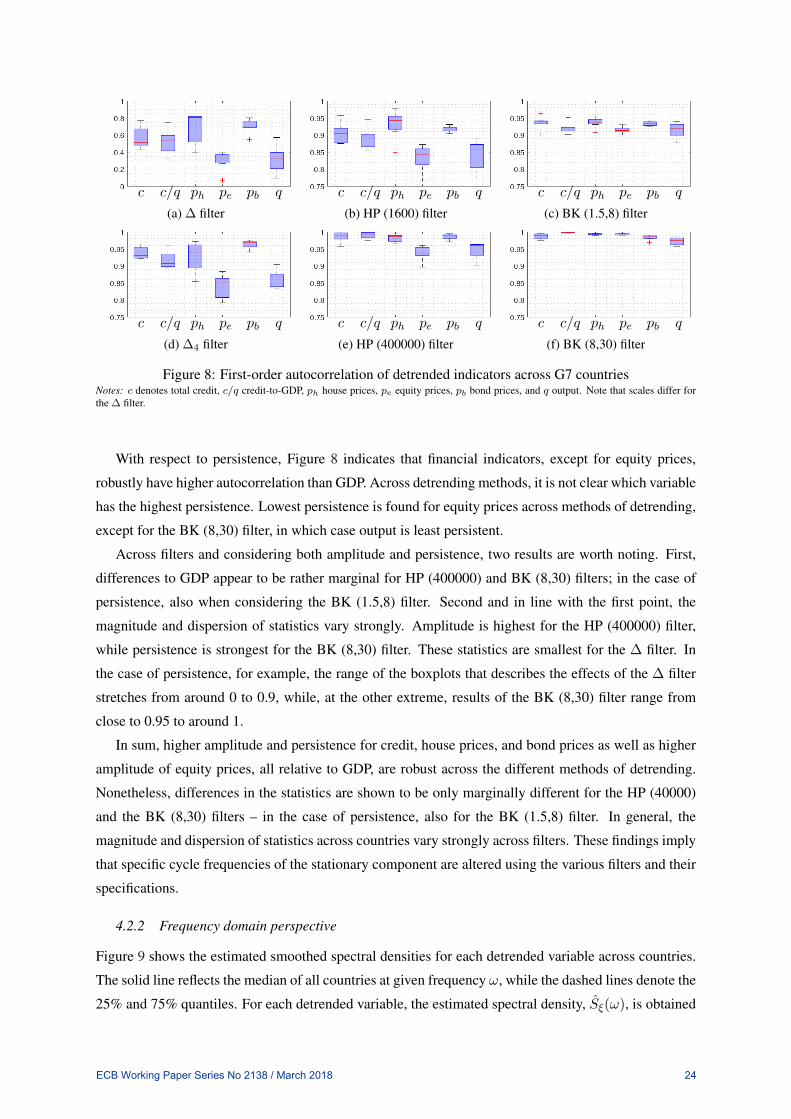
by cycles of duration close to 7 years for HP (1600) and BK (1.5,8) filters, around 20 years for the BK
(8,30) filter, and close to 30 years for the HP (400000) filter. Further and without assuming any DGP,
my empirical exercise reveals that these cycle durations are closely matched by the actual detrended
components, irrespective of the country or variable. Clearly, given the different variables (credit, credit-
to-GDP, house prices, equity prices, bond prices, and GDP) but also the different histories, laws, and
institutions of G7 countries, similar-duration cycles reflect strong evidence of spurious cycles, even if
the true underlying DGP is unknown. Still, unit root tests favour a DS process, as the null hypothesis
of a unit root cannot be rejected in most variable cases. Next to similar-duration cycles, I also find
that the strong amplification of medium-term frequencies of medium-term filters under a DS process is
consistent with my empirical results.
The first and fourth difference filters do not suffer from such distortions. Applying these, there is
clear evidence of longer (or more persistent) cycles in credit, credit-to-GDP, house prices, and bond
prices than in GDP; e.g., around 15 years for credit versus 6 years for GDP, on average across G7
countries. Equity price cycles have rather similar durations to business cycles. Further, I find different
durations of cycles across countries and variables. In the case of HP and BK filters, the durations of
cycles are distorted towards the expected lengths given a DS time series. Here, longer financial cycles
are still apparent, but differences to GDP become marginal. For instance in case of the HP (1600)
filter, my results suggest that on average GDP cycles are 6.2 years while credit cycles 7.4 years. I show
that the synchronisation of cycles in credit, credit-to-GDP, and house prices is more disperse across
countries and, on average, weaker than that of cycles in GDP, but stronger for cycles in equity and
bond prices.Using DPCoh, I find that the weaker synchronisation of cycles in credit and credit-to-GDP
across countries relates to medium-term fluctuations. For some country pairs, these cycles are negatively
related, cancelling out positively related cycles at other frequencies and consequently inducing weaker
overall synchronisation. Finally, higher amplitude of financial variables relative to GDP is found for all
methods of detrending.
This paper contributes to research on spurious cycles by pointing out the strong amplification of
cycles around 20 to 30 years when extracting medium-term frequencies with HP and band-pass filters.
Further, I provide first cross-country evidence on spurious cycles using HP and band-pass filters, for a
series of variables. Here, the study by A’Hearn and Woitek (2001) is closest. The authors, as well, ex-
plore the possibility of spurious cycles in a cross-country setup. However, they do not find any evidence,
which is due to their yearly sampling frequency and the consideration of business cycle frequencies that
ECB Working Paper Series No 2138 / March 2018 6

only lead to small distortions.7 This paper also relates to a recent study by Hamilton (2017), in which
he argues that one should never use the HP filter, as among others, the typical economic time series is
best approximated by a random walk, i.e., a DS time series. My paper extends his findings, first, by
providing evidence that band-pass filters are subject to a similar criticism as the HP filter and, second,
by providing evidence that also for a broad set of countries his conjecture about the typical economic
times series appears to hold.
Additionally, this paper contributes to the emerging strand of literature analysing the properties
of financial variables, for instance, relative to the characteristics of business cycle variables, as e.g.,
Claessens et al. (2011, 2012) or Aikman et al. (2015). First, I show that financial cycle facts, i.e., the
characteristics of financial variables to similarly detrended GDP, are broadly robust with respect to sev-
eral filtering procedures. Second, my results provide evidence that the weak synchronisation of credit
and credit-to-GDP cycles (see Schüler et al. (2017)) is partially driven by opposing medium-term de-
velopments. This is essential to better understand reciprocities across borders in the short- and long-run
and, thus, potential secondary effects of country-specific macroprudential policies. Economically, the
existence of such opposing cycles could be related to different degrees of financial market liberalisa-
tion across countries, say, in terms of mortgage credit standards (see Favilukis, Kohn, Ludvigson and
Van Nieuwerburgh (2013)), which can be ascribed to medium-term developments. Finally, my findings
suggest that financial variables, except for bond prices, are rather characterised by stochastic trends.
Different natures of trends have direct implications not only for detrending, but also for the modelling
of such variables. That is, in the case of TS financial variables, shocks to the latter are small, infrequent,
and have only transitory effects. In contrast to this, in the case of DS financial variables, shocks to these
indicators are large, frequent, and highly persistent. This has major implications for the conduct and
evaluation of macroprudential policies. It is only in the case of a DS process that the modelling and
identification of the shocks becomes critical (see Murray and Nelson (2000)).
The structure of the paper is as follows: In Section 2, I briefly exemplify the consequences of
spurious cycles for empirical analyses. In Section 3, I introduce the methods of detrending and shed
light on their effects on TS and DS time series. Section 4 applies these filters to data of G7 countries,
starting with the visual inspection and formal unit root testing of the series, followed by a discussion
of amplitude, length, and finally synchronisation both from a time and frequency domain perspective.
Section 5 concludes.
2 CONSEQUENCES OF SPURIOUS MEDIUM-TERM CYCLES
To illustrate the consequences of spurious medium-term cycles, I provide two examples in this section.
First, I construct gaps using different HP filter specifications on simulated data, and second, I discuss7For instance, researching cycles between 2 years, the minimum frequency available using yearly data, and 15 years, means
considering the region π to π7.5
for yearly data and π/4 to π/30 for quarterly data. The latter region, i.e., using quarterly data,is located closer to the trend (closer to frequency 0) that is more prone to the distortions discussed in the paper. Specifically, ascan be seen in the Figure 2 of A’Hearn and Woitek (2001, p. 327), the distortion visible in the power transfer function is muchmore modest than the ones discussed in this paper, which is related to the sampling frequency. The peak of their power transferfunction of the HP (100) filter is around 3.2, while it is around 204 for the HP (400000). For their BK filter (K = 6) the peakof the power transfer function is below 1.2, while 120 for the BK (8,30) filter (see Section 3).
ECB Working Paper Series No 2138 / March 2018 7

the consequences of spurious medium-term cycles for the credit-to-GDP gap in the case of the US and
France. In both examples, I discuss the distortions of filters that, one the one hand, are in line with the
empirical results of this paper and, on the other hand, can be motivated under a DS DGP.
2.1 Simulated data
The HP-filtered gaps extracted from the simulated data and the true gap itself are shown in Figure 1.
The upper panel depicts the true gap, the lower left panel illustrates the HP (1600) gap (together with the
true gap), and the lower right panel shows the HP (400000) gap (along with the true and the HP (1600)
gap). The data is simulated from an autoregressive model fitted to the changes in the US credit-to-GDP
ratio to capture realistic dynamics of financial variables in the true gap. Thus, in this exercise assume
that the US credit-to-GDP ratio is a difference stationary process. I simulate 180 observations, which is
similar to the sample period available for this paper.8
50 100 150
-0.01
0
0.01
0.02
(a) True gap
50 100 150
-0.02
0
0.02
(b) HP (1600) gap
50 100 150-0.1
0
0.1
(c) HP (400000) gap
Figure 1: Simulated dataNotes: The HP-filtered gaps are obtained by detrending the level of the simulated data with smoothing parameters 1,600 and 400,000 respec-tively. I simulate 180 observations; similar to the sample period available for this study. For further details, please see Appendix A.1.
The amplification of specific cycle frequencies (spurious cycles) can be noticed via the relative
increase in the variance of the HP filtered gaps, where the HP (400000) gap has the highest variance
and the true gap the lowest variance. For instance, the overall variance of the HP (400000) gap is more
than 18 times larger than the overall variance of the HP (1600) gap. This is broadly in line with the
theory that predicts a maximum factor of amplification of a small frequency range of roughly 13 for the
HP (1600) filter and about 204 for the HP (400000) filter. In the first case, cycles of length around 30
observations are most strongly amplified and in the second case frequencies close to 120 observations
are most strongly amplified. Note that the longest cycle observed for the HP (400000) gap is actually
around 80 observations, indicating that this reflects the longest duration cycle in the simulated data.
As Figure 1 suggests, the amplification implies that shorter frequencies become relatively muted,
leading to distortions that are stronger when considering the HP (400000) filter. Or, put differently,8See Appendix A.1 for further details on the simulation procedure.
ECB Working Paper Series No 2138 / March 2018 8

while shorter-term movements of the true gap are to some degree still observed in the HP (1600) gap,
they are almost completely muted in the HP (400000) gap.
The true gap, in this example, is sometimes also referred to as a cycle in growth rates (see Harding
and Pagan (2005)). Such a term might suggest that there exists a (possibly not perfect) mapping from
the HP-filtered gaps to the true gap via growth rates. That is, a positive (possibly constant) true gap
would imply a steady expansion of the HP-filtered gaps. Of course, this is correct, albeit irrelevant if
the true DGP is DS. Under a DS DGP, the HP filter amplifies certain frequencies of the true fluctuations
that are determined by the selected smoothing parameter. This creates a spurious gap, i.e., artificial
expansionary and contractionary periods, from which economists aim to infer, for example, about the
build-up of imbalances. The derived gaps, however, are entirely artificial and merely reflect the a priori
specification of the filter. As is apparent from this example, the HP (1600) and HP (400000) gaps
suggest different periods of positive and negative deviations from trend, leading, in a real world setting,
to differing regulatory responses or conclusions, which in both cases would not be in line with the true
gap.
2.2 Credit-to-GDP gap: US and France
Next, consider the real-time Basel III credit-to-GDP gaps of the US and France portrayed in Figure 2
along with the starting dates (black vertical lines) of systemic banking crises as defined by Laeven and
Valencia (2012). The two examples highlight well the negative consequences of spurious medium-term
cycles, as movements in the latter gaps have direct implications for the setting of CCyBs.9
70 74 78 82 86 90 94 98 02 06 10
-2
0
2
(a) US
70 74 78 82 86 90 94 98 02 06 10
-1
0
1
2
(b) France
Figure 2: Credit-to-GDP gapNotes: Credit-to-GDP gaps are constructed using an one-sided HP filter with smoothing parameter 400,000. Series are standardised to unitvariance. Grey shaded areas are NBER dates of recession. Black vertical lines indicate the onset of systemic banking crises as defined byLaeven and Valencia (2012).
While both country gaps are positive in the run-up to the GFC, which would support the indicators’
use to inform the setting of CCyBs – as the latter should have also been positive to limit the build-up of
imbalances through excess aggregate credit growth –, the movements during and after the GFC indicate
well the problems related to the amplification of medium-duration cycles. First, the US gap does not
indicate the materialisation of systemic risk immediately after the shock hit the economy, but takes until
the end of 2009 to close. Second, and even more dramatically, the French gap increases after the shock9Note that, throughout the study, I analyse the effects using a two-sided HP filter, i.e., employing all sample information.
The Basel III gaps, however, are constructed exploiting a one-sided, i.e., asymmetric, HP filter. I discuss differences betweenthe two approaches for the simulated data in Appendix A.1 and for the credit-to-GDP gaps of the G-7 countries in Section 4.1.
ECB Working Paper Series No 2138 / March 2018 9
hit the French economy in 2008, wrongly suggesting that the CCyB should have been raised over that
period. However, note the two small downturns visible around 2008 and 2009. It can be argued that
these reflect relevant cyclical fluctuations for informing the use of the CCyB, although they are masked
by the amplified medium-term cycle.
Thus, while the parameter of 400,000 leads to a gap for the US that peaks before the GFC and also
before the saving and loans crisis in 1988, the gap of France does not indicate any strong imbalances
prior to the GFC. Hence, due to the strong amplification of medium-term frequencies over shorter-term
ones, the extracted gaps are at high risk of not being relevant to the policy task or research question at
hand. These observations call into question the common assumption of “one smoothing parameter – or
one frequency window in the case of band-pass filters – fits all countries” approach, particularly when
considering cycles in the medium-term.10
3 DETRENDING METHODS AND THEIR EFFECTS ON TREND AND
DIFFERENCE STATIONARY TIME SERIES
In the business cycle context it is common practice to decompose real variables, such as output, into a
secular (or trend) component and a stationary, possibly cyclical, component. With respect to financial
variables, the same approach has been taken. For instance, researchers and policy makers aim at identi-
fying a credit gap measure that should indicate the build-up of excesses or imbalances in order to inform
countercyclical macroprudential policies.
In these exercises, a stationary component is identified by deviations from a non-stationary secular
component. A non-stationary secular component in credit (possibly over GDP) may arise, for example,
from a continued financial deepening or integration that allows an even further expansion of the credit
volume, i.e., reflecting developments with permanent effects. The stationary component is regarded as
the outcome of transitory, possibly persistent, shocks within an economy, such as phases of high risk
aversion triggered by certain financial shocks. It is possible to imagine that shocks to the stationary
component may also affect the trend, leading to permanent effects of shocks.
One way to think of this is to decompose (the log of) credit or any other trending series, say yt, into
the sum of such trend and stationary component, for instance, as
yt = τt + ψt, (1)
where t = 1, . . . , T , τt reflects a non-stationary trend and ψt a stationary, non-deterministic, and
possibly cyclical component. In this framework, ψt can be referred to as the gap, meaning that a
permanent component, τt, is removed from yt; as is the case with the credit-to-GDP or output gap.
To analyse the effects of filters on ψt, I consider two data generating processes (DGPs) that have
gained prominence in discussions about the trend, i.e., τt, in output (see, for instance, Nelson and
Plosser (1982)): trend (TS) and difference (DS) stationary DGPs. Both can be nested in Equation (1)10Of course, due to country specificities the credit-to-GDP gap could possibly not be the relevant indicator for informing the
CCyB for France. However, different transformations of this indicator (see Appendix A.2.1) suggest the existence of relevantmovements that signal the downturn during the GFC.
ECB Working Paper Series No 2138 / March 2018 10

and be formalised as
TS: yt = α+ βt+ ψt (2)
DS: yt = α+ yt−1 + ψt, (3)
where α is an intercept (or possibly a drift parameter in Equation (3)), t a deterministic trend and β
a slope coefficient of the trend. In the TS case, movements in ψt do not affect the trend. In contrast, in
the DS case, movements in ψt almost completely determine the evolution of the trend.
In the framework proposed by Harding and Pagan (2005), ψt in Equation (2), is called a growth
cycle and ψt in Equation (3) is referred to as a cycle in growth rates. The representation in Equation (1)
indicates that such a distinction is not clear-cut, which is acknowledged by Harding and Pagan (2005),
who regard Equation (3) as a special case of growth cycles. Clearly, the results of this section are
sensitive to the assumptions made on the DGP.11
While both DGPs give rise to the “typical spectral shape” discussed by Granger (1966) when esti-
mating the spectral density of yt, the effects of filters on ψt vary depending on the two DGPs. Depending
on the two DGPs, methods may generate spurious cycles in ψt by amplifying certain cycle frequencies
relative to others, thus biasing the original stationary component.
Below, I first delineate the filters considered and, subsequently, discuss their effects on TS and DS
time series. Some final remarks conclude this section.
3.1 Methods of detrending
I consider three different filters and, for each, two different specifications. The first is the difference
filter, the second the Hodrick and Prescott (1981, 1997) (HP) filter, and the third the Baxter and King
(1999) (BK) filter. The analysis of different specifications is explained by the different detrending
approaches adopted by researchers and policy makers when analysing business and financial cycles.
Standard filters in the business cycle context (using a quarterly sampling frequency) are the first dif-
ference (∆) filter, the HP filter with a smoothing parameter of 1,600 (HP (1600)), and the BK filter
extracting frequencies from 1.5 to 8 years (BK (1.5,8)).12 The fourth difference (∆4) filter, the HP filter
with a smoothing parameter of 400,000 (HP (400000)), and the BK filter extracting cycles of duration
8 to 30 years (BK (8,30)) have been recently advocated in the financial cycle context aiming to extract
medium-term cycles. For instance, the ∆4 filter has been employed by Drehmann et al. (2012), Strohsal
et al. (2015a), and Verona (2016). The HP (400000) is recommended by the Basel III regulations for
constructing the credit-to-GDP gap and is used, for instance, by Anundson et al. (2016). Focussing on
cycles between 8 and 30 years by means of a band-pass filter, is suggested by Drehmann et al. (2012)
and, for instance, used by Meller and Metiu (2015, forthcoming).
Below, let ξt denote the detrended component of yt, i.e., the estimate of ψt.11For instance, using the classic growth cycle definition, Murray (2003) shows that if yt is driven by an integrated trend, i.e.,
τt = α+ τt−1 + ζt with ζt stationary and ζt uncorrelated with ψt, implies that spurious cycles emerge as the first differenceof the trend is passed through the filter. Here, the properties of the filtered series are strongly determined by the trend in theunfiltered series. In this framework spurious cycles emerge due to an amplification of specific frequencies in ζt and not ψt.
12The ∆ filter has been used by Schularick and Taylor (2012), Aikman et al. (2015), and Schüler et al. (2015, 2017) in thefinancial cycle context.
ECB Working Paper Series No 2138 / March 2018 11

Two specifications of the difference filter
I analyse both the first and fourth difference filter. Let ∆i = (1− Li). The two filters are
ξ∆t = ∆yt = (1− L)yt = yt − yt−1 and (4)
ξ∆4
t = ∆4yt = (1− L4)yt = yt − yt−4. (5)
Two specifications of the Hodrick and Prescott (1981, 1997) filter
I consider two smoothing parameters: λ = 1,600 and λ = 400,000. The smoothing parameter, λ,
controls the importance of the penalty term attached to the degree of smoothness of the extracted trend.
A parameter of 400,000 leads to a much smoother trend than 1,600.
Most commonly the HP filter is written in the following form:
min[τt]Tt=1
[T∑t=1
(yt − τt)2 + λ
T∑t=2
((τt+1 − τt)− (τt − τt−1))2
], λ > 0. (6)
For the analysis of this paper, however, it is convenient to rewrite the latter minimisation problem into
a form that directly yields the detrended observations, ξt (see, for example, King and Rebelo (1993)):
ξHP(λ)t =
[(1− L)2(1− L−1)2
(1− L)2(1− L−1)2 + 1/λ
]yt. (7)
Two specifications of the Baxter and King (1999) filter
I use the BK filter to extract two different frequency bands: first, disentangling fluctuations between 1.5
and eight years and, second, fluctuations between eight and 30 years.
The extracted component is obtained through
ξBK(π/(2ω1),π/(2ω2))t = aK(L)yt, (8)
where (π/(2ω1), π/(2ω2)) denotes the frequency band in years with π/(2ω1) < π/(2ω2), aK(L) =∑Kk=−K akL
k is a symmetric lag polynomial, and ak = a−k a time-invariant symmetric linear weight.
In contrast to the ideal band-pass filter that uses an infinite number of weights, the weights of the BK
filter are truncated at lag K. Due to this, Baxter and King (1999) introduce a normalising constant such
that aK(1) =∑K
k=−K ak = 0, which implies that the filter may neglect long-run trends. More formally,
ak = bk + θ, (9)
where θ is the normalising constant and bk the time invariant linear weight of the band-pass filter. θ
is defined to be (−∑K
k=−K bk)/(2K + 1). Further,
bk =
ω1 − ω2
πif k = 0
sin(ω1k)− sin(ω2k)
πkif k 6= 0
(10)
For fixed K, the researcher defines the frequency band that she would like to consider by choosing
ω1 > ω2. Using a quarterly sampling frequency, filtering frequencies between 1.5 and 8 years implies an
ECB Working Paper Series No 2138 / March 2018 12

ω1 = π/2·(1.5)−1 and an ω2 = π/2·(8)−1; 8 to 30 years an ω1 = π/2·(8)−1 and an ω2 = π/2·(30)−1.
For the two specifications, I choose K = 40 which is larger than the parameter that has been suggested
by Baxter and King (1999) for analysing business cycles (K = 12), but has been considered by Murray
(2003) for the latter purpose. The filter captures medium-term cycles more precisely when using more
lags.
3.2 The filters’ effects on trend and difference stationary time series
To discuss the effects of the filters on the two data generating processes, I first introduce the concept of
power transfer functions (PTFs) which can be used to describe how filtering modifies certain frequencies
of a stationary time series and can, thus, indicate induced cycles, i.e., specific frequencies that are
amplified relative to others.13
3.2.1 The power transfer function and induced cycles
Assume that ψt is a stationary stochastic process with an autocovariance generating function defined as
gψ(z) ≡∑∞
t=−∞ γtzt, where z denotes a complex scalar and γt the autocovariances. γ0 refers to the
variance of ψt. The spectral density of ψt is then defined as
Sψ(ω) ≡ 1
2πgψ(e−iω), (11)
where i is the imaginary unit and ω ∈ [−π, π] the cycle frequency in radians. Filtering ψt with a
time-invariant filter that has absolutely summable weights, say ξt =∑∞
j=−∞ hjψt−j , implies that the
spectral density is altered via a transfer function. This transfer function can be denoted by h(e−iω) and
the exact relation between the spectral density of ψt and the spectral density of the filtered series is
Sξ(ω) = H(ω) · Sψ(ω), (12)
where H(ω) ≡ |h(e−iω)|2 is referred to as the power transfer function. It completely describes the
change in the relative importance of the cyclical components in ψt.14 If H(ω) > 1, the amplitude of
the cycle component ω of ψt is increased. In the case H(ω) < 1, the amplitude of the respective cycle
component is dampened. Such amplification or dampening of frequencies in the stationary component
ψt gives rise to spurious or artificial cycles.
Note that, while ψt is stationary, the original time series, yt, might not be. In this case, i.e., when the
filter is applied to a trending variable, the PTF describing the change of cycle frequencies for ψt might
differ from the PTF of the filter, depending on the source of nonstationarity. This is discussed below.13All frequency domain results are interpreted assuming quarterly sampling frequency, which is the frequency of variables
used in this study.14The transfer function can be decomposed into gain and phase, where the square of the gain is the power transfer function,
i.e., h(e−iω) = |h(e−iω)|e−iΘ(ω). Θ(ω) refers to the phase. Note that for symmetric linear filters, such as the HP filter thephase is zero. For the first difference filter, it is not. Nonetheless, I refrain from a discussion of phase, as it is not relevant tothe analysis of this paper. Changes in the importance of frequencies are fully described by the power transfer function and,for instance, the synchronisation of cycles across countries is analysed using the same filter across countries, in which case thesame phase shift applies to all variables.
ECB Working Paper Series No 2138 / March 2018 13
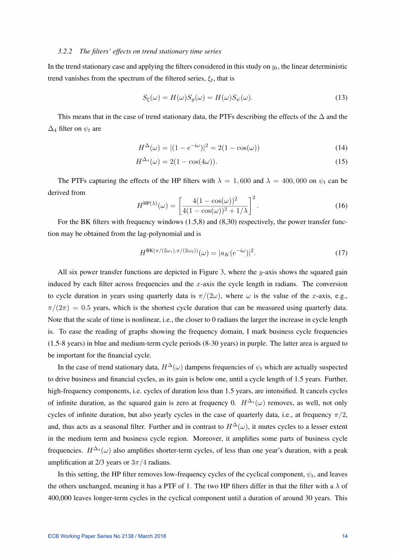
3.2.2 The filters’ effects on trend stationary time series
In the trend stationary case and applying the filters considered in this study on yt, the linear deterministic
trend vanishes from the spectrum of the filtered series, ξt, that is
Sξ(ω) = H(ω)Sy(ω) = H(ω)Sψ(ω). (13)
This means that in the case of trend stationary data, the PTFs describing the effects of the ∆ and the
∆4 filter on ψt are
H∆(ω) = |(1− e−iω)|2 = 2(1− cos(ω)) (14)
H∆4(ω) = 2(1− cos(4ω)). (15)
The PTFs capturing the effects of the HP filters with λ = 1, 600 and λ = 400, 000 on ψt can be
derived from
HHP(λ)(ω) =
[4(1− cos(ω))2
4(1− cos(ω))2 + 1/λ
]2
. (16)
For the BK filters with frequency windows (1.5,8) and (8,30) respectively, the power transfer func-
tion may be obtained from the lag-polynomial and is
HBK(π/(2ω1),π/(2ω2))(ω) = |aK(e−iω)|2. (17)
All six power transfer functions are depicted in Figure 3, where the y-axis shows the squared gain
induced by each filter across frequencies and the x-axis the cycle length in radians. The conversion
to cycle duration in years using quarterly data is π/(2ω), where ω is the value of the x-axis, e.g.,
π/(2π) = 0.5 years, which is the shortest cycle duration that can be measured using quarterly data.
Note that the scale of time is nonlinear, i.e., the closer to 0 radians the larger the increase in cycle length
is. To ease the reading of graphs showing the frequency domain, I mark business cycle frequencies
(1.5-8 years) in blue and medium-term cycle periods (8-30 years) in purple. The latter area is argued to
be important for the financial cycle.
In the case of trend stationary data, H∆(ω) dampens frequencies of ψt which are actually suspected
to drive business and financial cycles, as its gain is below one, until a cycle length of 1.5 years. Further,
high-frequency components, i.e. cycles of duration less than 1.5 years, are intensified. It cancels cycles
of infinite duration, as the squared gain is zero at frequency 0. H∆4(ω) removes, as well, not only
cycles of infinite duration, but also yearly cycles in the case of quarterly data, i.e., at frequency π/2,
and, thus acts as a seasonal filter. Further and in contrast to H∆(ω), it mutes cycles to a lesser extent
in the medium term and business cycle region. Moreover, it amplifies some parts of business cycle
frequencies. H∆4(ω) also amplifies shorter-term cycles, of less than one year’s duration, with a peak
amplification at 2/3 years or 3π/4 radians.
In this setting, the HP filter removes low-frequency cycles of the cyclical component, ψt, and leaves
the others unchanged, meaning it has a PTF of 1. The two HP filters differ in that the filter with a λ of
400,000 leaves longer-term cycles in the cyclical component until a duration of around 30 years. This
ECB Working Paper Series No 2138 / March 2018 14

Radians
0 π/4 π/2 3π/4 π
PTF
0
1
2
3
4
Δ filter
Δ4 filter
Radians
0 π/4 π/2 3π/4 π
PTF
0
1
2
3
4
HP (1600)
HP (400000)
Radians
0 π/4 π/2 3π/4 π
PTF
0
1
2
3
4
BK (1.5,8)
BK (8,30)
Figure 3: (Trend) stationary time series: power transfer functions, H(ω)Notes: The blue area marks business cycle frequencies (1.5-8 years) and the purple area medium-term cycles (8-30 years) assuming quarterlydata. PTF denotes the power transfer function. Results of the BK filter use K = 40.
contrasts with the cyclical component obtained by the HP filter with a λ of 1,600 contains cycles of up
to roughly 8 years.
HBK(π/(2ω1),π/(2ω2))(ω) with K = 40 approximates a gain of one for the frequency band specified.
In black, I show the specification that leaves frequencies between 1.5 and 8 years in ψt and in red the
specification that is supposed to leave medium-term cycles in the stationary component. In the case of
the latter, there is a marginal amplification of cycles of around 13 years’ duration in the region where
the PTF peaks at a value greater than one.
In sum, given TS time series, both difference filters induce cycles in ψt. The ∆ filter amplifies
cycles at high frequencies, but not at business and financial cycle frequencies. The ∆4 filter amplifies
cycles at around 2 and 2/3 years, with the former implying induced cycles in the business cycle range.
In contrast, the HP and BK filters represent close approximations to the ideal band-pass filters when
considering their effects on the stationary component, ψt, for which the gain of the PTF is around one.
The HP filter with a smoothing parameter of 400,000 implies that longer-term cycles are left in the
stationary component. Both specifications of the BK filter emphasise cycles of desired length in ψt.
3.2.3 The filters’ effects on difference stationary time series
In the difference stationary case, the effects of the filters on ψt change. They operate as a two-step
linear filter, in which case yt, in a first step, is differenced to render the series stationary and, in a second
step, smoothed with the remainder of the filter. Remainder means that the application of such filters in
this setting “uses up” one difference operator (see, for example, Cogley and Nason (1995) and Murray
(2003)). Thus, the transfer function of interest, say J(ω), which describes the effects on the stationary
component ψt, can be derived by
Sξ(ω) = H(ω)Sy(ω) = J(ω)S∆y(ω) = J(ω)Sψ(ω), (18)
where J(ω) = H(ω)/H∆(ω).
ECB Working Paper Series No 2138 / March 2018 15
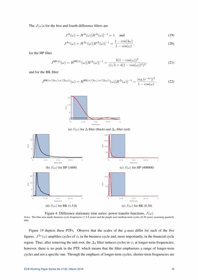
The J(ω)s for the first and fourth difference filters are
J∆(ω) = H∆(ω)[H∆(ω)]−1 = 1 and (19)
J∆4(ω) = H∆4(ω)[H∆(ω)]−1 =1− cos(4ω)
1− cos(ω), (20)
for the HP filter
JHP(λ)(ω) = HHP(λ)(ω)[H∆(ω)]−1 =8(1− cos(ω))3
(1/λ+ 4(1− cos(ω))2)2, (21)
and for the BK filter
JBK(π/(2ω1),π/(2ω2))(ω) = HBK(π/(2ω1),π/(2ω2))(ω)[H∆(ω)]−1 =|aK(e−iω)|2
1− cos(ω). (22)
Radians
0 π/4 π/2 3π/4 π
PTF
01
5
10
15
(a) J(ω) for ∆ filter (black) and ∆4 filter (red)
Radians
0 π/4 π/2 3π/4 π
PTF
0
5
10
(b) J(ω) for HP (1600)
Radians
0 π/4 π/2 3π/4 π
PTF
0
50
100
150
200
(c) J(ω) for HP (400000)
Radians
0 π/4 π/2 3π/4 π
PTF
0
5
10
15
(d) J(ω) for BK (1.5,8)
Radians
0 π/4 π/2 3π/4 π
PTF
0
50
100
(e) J(ω) for BK (8,30)
Figure 4: Difference stationary time series: power transfer functions, J(ω)Notes: The blue area marks business cycle frequencies (1.5-8 years) and the purple area medium-term cycles (8-30 years) assuming quarterlydata.
Figure 19 depicts these PTFs. Observe that the scales of the y-axes differ for each of the five
figures. J∆4(ω) amplifies cycles of ψt in the business cycle and, more importantly, in the financial cycle
region. Thus, after removing the unit root, the ∆4 filter induces cycles in ψt at longer-term frequencies;
however, there is no peak in the PTF, which means that the filter emphasises a range of longer-term
cycles and not a specific one. Through the emphasis of longer-term cycles, shorter-term frequencies are
ECB Working Paper Series No 2138 / March 2018 16
almost completely muted. In contrast, the ∆ filter does not change the spectrum of the the stationary
component, ψt. The PTF is 1 for all frequencies. Assuming a DS process, the first difference filter thus
removes, first, the source of nonstationarity and, then, leaves the stationary component unaltered.15
In the case of the two J(ω)s of the HP filter, both PTFs peak and therefore magnify specific fre-
quencies. The higher the smoothing parameter is, the more strongly are cycles in ψt magnified – up
to around 13 times employing a parameter of 1,600 and up to roughly 204 times using a parameter of
400,000. The HP filter may therefore introduce spurious cycles into the stationary component, i.e., em-
phasise cycles that are present in the data but may not be important relative to other fluctuations present
in the stationary component or not of relevance to the research question at hand. Note that the frequency
that is emphasised can be derived from ωmax = arccos(1 −√
0.75/λ). Accordingly, in the case of a
λ = 1,600, cycles of lengths around 7.5 years in ψt are emphasised, whereas for λ = 400,000 cycles of
lengths around 30 years are emphasised.
Similarly, the two J(ω)s of the BK filters peak and, thus, emphasise specific cycles in ψt. The filter
(1.5,8) magnifies durations of around 6.2 years with a factor of around 18 and the (8,30) of around 18
years with a factor of approximately 120. In contrast to the HP filter, the BK filter cancels all shorter-
term frequencies that have not been included in the specification, i.e., below 1.5 and below 8 years
respectively.
In sum, given a DS process, the HP filter may induce cycles of around 7.5 and 30 years in the
stationary component for a smoothing parameter of 1,600 and 400,000 respectively. The BK filters
emphasise frequencies of roughly 6.2 and 18 years’ duration in the stationary component when filtering
(1.5,8) and (8,30) years respectively. The ∆4 filter amplifies longer-term cycles, whereas the ∆ filter
does not alter the cyclical component at all. These insights highlight the importance of the a priori
choice of the HP smoothing parameter or the BK frequency window for the detrending of DS time
series as they lead to a focus on specific fluctuations of the cyclical component.
3.2.4 Some remarks
It is worth noting that the effects of filters on DS time series have broad implications, that is, Cogley
and Nason (1995) show that the effects of filters on near unit root trend stationary time series are similar
to the effects on difference stationary time series.
Further, Pederson (2001) points out that effects of the HP and BK filters on DS time series need to
be discriminated from the Slutzky effect. The Slutzky effect is defined as distortions that occur when
filtering stationary data. Or, put differently, the PTFs of the filters themselves show peaks and, thus,
induce spurious cycles by emphasising specific frequencies relative to others; as is with the difference
filters. This is not the case for the HP and BK filters, which both approximate an ideal band-pass filter
for the specified frequency range. Even though the distortions of these filters do not coincide with the
Slutzky effect, their implications are important, especially when considering medium-term fluctuations.15Note, the ∆ filter is the non-distorting filter in this application, as I assume a first difference stationary process in this
exercise (see Equation (3)). This is in line with Hamilton (2017)’s argument that a typical economic time series is bestapproximated by a random walk and by the empirical evidence provided in this paper. Clearly, if the true DGP would be a ∆4
process the fourth difference filter would be best suited.
ECB Working Paper Series No 2138 / March 2018 17
At last, the exposition in this section emphasises the importance of knowing the true DGP for choos-
ing the “correct” filter, i.e., the one that either minimally distorts the cyclical properties of the underlying
series or extracts the fluctuations of interest. However, as the true DGP cannot be known in practice,
the following empirical exercise aims to provide evidence on distortions that filters induce in actual
economic time series, without the need to assume a specific DGP.
4 FINANCIAL CYCLE FACTS ACROSS G7 COUNTRIES
Having shed light on the theoretical properties of filters, I now turn to discuss the effects of applying
them to financial and business cycle variables of G7 countries. To begin with, I introduce the data,
depict their (log-)levels and detrended components, and formally test whether there is evidence against
the hypothesis of a unit root with possible drift (DS) using the alternative hypothesis of a TS DGP.
Subsequently, I examine the amplitude and length of financial cycle variables relative to business cycles.
Thereafter, I reflect on the synchronisation of financial cycle variables across countries, also contrasting
with the synchronisation of business cycles. In both exercises, I first explore a time and second a
frequency domain perspective. I employ both perspectives as each highlights different features of the
detrended components.
4.1 Data and some notes on filtering
I use the dataset by Schüler et al. (2017) which includes quarterly data on credit, house prices, equity
prices, and bond prices, augmented by the credit-to-GDP ratio. This set of variables reflects indicators
measuring financial cycles. The representative business cycle variable is GDP. The dataset covers G7
countries and spans the period from 1969Q1 to 2013Q4.
Credit, house prices, and credit-to-GDP reflect time series from the Bank of International Settle-
ments. Credit is total credit, and house prices are measured through residential property prices. For
equity prices, the main economic indicators database from the OECD is employed, except for the US,
in which case I use the S&P 500 index that is the standard variable in academic studies researching on
US equity markets. Corporate bond yields are taken from Global Financial Data and Haver Analytics.
GDP is also retrieved from the OECD main economic indicators database.16 All variables are in real
terms, log-transformed (except for credit-to-GDP), and deflated via the CPI index of the OECD main
economic indicators database where necessary. Seasonal adjustment is performed using Census X-12.
Note that bond yields are transformed to reflect bond prices as suggested in Schüler et al. (2017),
i.e., pb,t = 1/(1 + yb,t), where pb,t denotes the price and yb,t is the current yield of the respective bond
at time t. Such transformation assures, on the one hand, an interpretation of this variable similar to the
other asset price series considered and, on the other, allows for a similar process of deflating, which is
important when comparing cyclical structures across indicators.17
16For exact details please refer to the Appendix of Schüler et al. (2017)17The other option is to construct yearly inflation from the CPI indices and deduct those from the yields. However, as
highlighted in the previous section, the year-on-year filter runs the risk of emphasising specific cycles and inducing phaseshifts.
ECB Working Paper Series No 2138 / March 2018 18

Before proceeding with the analysis, it is useful to note that I employ the HP and BK filters using
whole sample information.18 However, the credit-to-GDP gap, as defined in the Basel regulations, is
actually constructed via a one-sided HP filter, i.e., an HP filter that is applied to an expanding sample.
This implies that only current and past information is employed. Of course, this is due to the restriction
that policy makers and regulators need to act in real time. For this study, I assume that all sample
information is available. A comparison of both approaches, i.e., constructing the credit-to-GDP gap
using a two- versus a one-sided HP filter, is given in Appendix A.2.2. Summarising, the dynamics of
the detrended series do not differ strongly. Most remarkable differences occur at the beginning of the
sample, when only few observations are available for the one-sided filter. In the case of France or Italy,
for instance, this leads to the outcome that the one-sided filtered series seems to be trending, possibly
biasing the analysis of the stationary component. Overall, the comparison suggests that the implications
derived from the two-sided filter carry over closely to the one-sided filter.
Finally, I compute the detrended component of the BK filter by extending the first and last observa-
tions by their respective value for several quarters, such that the sample period common to all filters is
longest.
4.1.1 Visual inspection of levels and detrended components
70 74 78 82 86 90 94 98 02 06 10
4.5
5
5.5
c
70 74 78 82 86 90 94 98 02 06 10
4.4
4.6
4.8
5
5.2
ph
70 74 78 82 86 90 94 98 02 06 10
4
4.5
5
5.5
pb
70 74 78 82 86 90 94 98 02 06 10
1
1.2
1.4
1.6
c/q70 74 78 82 86 90 94 98 02 06 10
4.5
5
5.5
6
pe
70 74 78 82 86 90 94 98 02 06 10
4.24.44.64.8
55.2
q
Figure 5: US’ financial and business cycle indicatorsNotes: Grey area depicts NBER dates of recessions. Black vertical lines indicate the onset of systemic banking crises as defined by Laevenand Valencia (2012). c denotes total credit, c/q credit-to-GDP, ph house prices, pe equity prices, pb bond prices, and q output.
Figure 5 depicts the US data in (log-) levels and Figure 6 shows the detrended components obtained
via the three filters as discussed in Section 3. Note that, for ease of exposition, the detrended series are
standardised to unit variance. The remaining country charts are placed in Appendix A.2.1.
Considering the time series graphs for the US, several conclusions can be drawn. With respect to the
levels, visual inspection suggests that all variables show trending behaviour. For equity prices (pe) this
evidence can be argued to be weakest, reminiscent of a random walk without drift. Further, while the
slope of the potential trends or drifts are positive for most series, these would be expected to turn out
negative for bond prices (pb).19
18While the HP and BK filters are employed using whole sample information, the difference filters – by construction,asymmetric filters – only use information at time period t together with t− 1 or t− 4.
19Clearly, ever declining real bond prices would be a puzzling phenomenon. As this study does not focus on finding
ECB Working Paper Series No 2138 / March 2018 19

Difference filters HP filters BK filters
70 74 78 82 86 90 94 98 02 06 10
-2
0
2
c70 74 78 82 86 90 94 98 02 06 10
-2
0
2
70 74 78 82 86 90 94 98 02 06 10
-2
0
2
70 74 78 82 86 90 94 98 02 06 10
-2
0
2
c/q70 74 78 82 86 90 94 98 02 06 10
-2
0
2
70 74 78 82 86 90 94 98 02 06 10-2
0
2
70 74 78 82 86 90 94 98 02 06 10
-2
0
2
ph70 74 78 82 86 90 94 98 02 06 10
-2
0
2
70 74 78 82 86 90 94 98 02 06 10
-2
0
2
70 74 78 82 86 90 94 98 02 06 10
-4
-2
0
2
pe70 74 78 82 86 90 94 98 02 06 10
-2
0
2
70 74 78 82 86 90 94 98 02 06 10
-2
0
2
70 74 78 82 86 90 94 98 02 06 10
-4
-2
0
pb70 74 78 82 86 90 94 98 02 06 10
-2
0
2
70 74 78 82 86 90 94 98 02 06 10
-2
0
2
70 74 78 82 86 90 94 98 02 06 10
-2
0
2
4
q70 74 78 82 86 90 94 98 02 06 10
-2
0
2
70 74 78 82 86 90 94 98 02 06 10
-2
0
2
Figure 6: Detrended US’ financial and business cycle indicators: ∆, HP (1600), BK (1.5,8) filter inblack, ∆4, HP (400000), and BK (8,30) filter in red
Notes: Grey area depicts NBER dates of recessions. Black vertical lines indicate the onset of systemic banking crises as defined by Laevenand Valencia (2012). Series are standardised to unit variance for ease of exposition. Each row refers to the variable indicated in the left handpanel. c denotes total credit, c/q credit-to-GDP, ph house prices, pe equity prices, pb bond prices, and q output. The BK filter is specifiedwith K = 40 and the cycles are computed by extending the first and last observations by their respective value for several quarters, such thatthe sample period common to all filters is longest.
Comparing the detrended components obtained with the ∆ to those derived with the ∆4 filter (see
Figure 6) leads to the conclusion that, on the one hand, short-term movements are muted using the ∆4
filter and, on the other, a slight phase shift is induced, i.e., turning points occur later for the ∆4 treated
version of each series. However, the lower frequency movements in both series seem to be similar.
Looking at the HP detrended series suggests that each specification of the filter leads to a different
cyclical pattern in each variable case. As expected, the HP filter with a λ of 400,000 captures longer-
term cycles than the filter with a λ of 1,600, but also mutes shorter-term fluctuations. Further, both
HP-filtered series look different from the fluctuations identified via the difference filters.
arguments for different theoretical mechanisms that generate the trending behaviour, I refrain from a further discussion alongthese lines.
ECB Working Paper Series No 2138 / March 2018 20

The two BK-filtered series, similar to the case of the HP filter, show different cyclical patterns. Of
course, this can be argued to be an artefact of the specifications, as the filter was required to separate
different cycle frequencies.
Interestingly, the BK (1.5,8)-filtered series resemble the HP (1600)-filtered series and the BK (8,30)-
filtered series resemble HP (400000) cycles, even though the BK filters completely mute shorter-term
fluctuations, for instance, in the case of the BK (8,30) filter, cycles shorter than eight years. Somehow,
this is reflected in a number of minor fluctuations in the HP-filtered series. Still, while cycles resemble
each other, they are not the same. For instance, credit reaches one of its historic peaks for both HP-
filtered series before the post-90 recession. In contrast, the BK (1.5,8)-filtered series only shows a
marginal deviation from trend.
Finally, note that the HP (400000) detrended component of equity prices and GDP contain by far
more shorter-term frequencies than in any other variable’s case.
In sum, all level series can be argued to show a trending behavior. The two difference filters produce
rather similar results when focussing on longer-term movements. Shorter-term movements are muted
using the ∆4 filter. Both HP and both BK filter calibrations deliver different cycles for all variables,
which are also different from the cycles obtained using the difference filters. Nonetheless, there is some
similarity between the HP and BK filter when comparing the cycles for the shorter-term frequencies, on
the one hand, and comparing the fluctuations of the longer-term cycles, on the other. These observations
are broadly consistent across G7 countries. It is only in the case of Japan that the trends in certain
variables are characterised by breaks, e.g., for house prices (ph), in which case no clear trend behaviour
is visible.
4.1.2 Are financial cycle variables trend or difference stationary?
This section explores for each variable whether it is possible to reject the null of unit root with drift
against the alternative of trend stationarity, which, as indicated, has important implications for distor-
tions induced by filters. More precisely, I use the following version of the augmented Dickey Fuller
test: under the null the series has a unit root with drift, i.e.,
yt = α+ yt−1 +
p∑i=1
θi∆yt−i + ηt (23)
where the p-lagged differences account for serial correlation and ηt is an iid normal error. Under the
alternative, I specify the model as
yt = α+ βt+ ρyt−1 +
p∑i=1
θi∆yt−i + ηt. (24)
Thus, I test the joint restriction that β = 0 and ρ = 1 using an F -test.20 Clearly, such a test cannot
completely determine whether a time series follows a stochastic or deterministic trend. First, the test20Note this test is similar to the test used in Murray and Nelson (2000) who explore whether the trend in US GDP is
deterministic or stochastic. The current test, however, differs in that I specify the DGP under the null to be a unit root withlinear drift. Murray and Nelson (2000) allow in their specification for a unit root with quadratic drift, which I argue does notreflect the trend observed in the data just discussed.
ECB Working Paper Series No 2138 / March 2018 21

suffers from low power against local alternatives. Second, breaks in the trend can lead to an under-
rejection of the null that could possibly be a factor, for instance, in the case of Japan. Nonetheless, the
current formulation of the ADF test gives initial evidence for one of the two data generating processes
which is augmented by details on the spectral densities of the detrended components in the following
parts.
Table 1: Augmented Dickey Fuller F -test
Variable AR Test Nominal Variable AR Test NominalCountry lag statistic p-value Country lag statistic p-value
Credit (c) Equity prices (pe)Canada 2 5.45 0.097 Canada 1 6.29 0.053Germany 1 13.54 0.001 Germany 1 5.87 0.072France 1 6.53 0.045 France 1 3.84 0.325Italy 2 1.88 0.778 Italy 1 4.02 0.285Japan 2 3.85 0.323 Japan 1 2.40 0.658UK 3 1.64 0.840 UK 1 3.91 0.310US 2 5.06 0.128 US 0 3.95 0.300Credit-to-GDP (c/q) Bond prices (pb)Canada 1 2.59 0.615 Canada 1 6.32 0.052Germany 1 2.15 0.716 Germany 1 9.79 0.004France 1 1.60 0.850 France 1 7.36 0.024Italy 1 4.26 0.229 Italy 1 7.36 0.024Japan 2 2.12 0.722 Japan 2 6.84 0.036UK 3 2.18 0.709 UK 2 7.26 0.026US 2 3.72 0.354 US 1 5.31 0.108House prices (ph) GDP (q)Canada 1 1.79 0.800 Canada 1 5.12 0.123Germany 1 3.70 0.358 Germany 1 6.63 0.042France 2 4.51 0.184 France 0 4.93 0.140Italy 1 7.43 0.023 Italy 4 6.67 0.041Japan 1 2.22 0.700 Japan 0 18.03 0.001UK 1 4.64 0.170 UK 0 1.23 0.933US 2 7.15 0.029 US 1 1.39 0.899
Notes: AR lags are chosen via minimising Schwarz (1978) information criterion over lags 0 to 12. Teststatistic refers to an F -test as described in the text. Nominal p-values are obtained by linear interpo-lation from tables that have been generated for a range of sample sizes and significance levels usingMonte Carlo simulations of the null model with Gaussian innovations and five million replications persample size.
The outcomes of the ADF tests are depicted in Table 1. Note that the AR lags are chosen by min-
imising the Schwarz (1978) information criterion that has been argued to produce roughly correctly
sized ADF tests (Hall (1994)).
Three results stand out: First, tests on credit-to-GDP (c/q) provide the weakest evidence against the
null hypothesis of a unit root, as it cannot be rejected for any country case at any given significance level,
while for the remaining variables the null hypothesis is at least rejected in two out of the seven country
cases using the ten percent significance level. This marks a strong result, as precisely credit-to-GDP is
recommended by the Basel regulations to be used with the HP (400000) filter and, thus, a gap measure
could be at high risk of representing an artefact of the method of detrending. Second, evidence against a
unit root with drift is greatest for GDP (q, rejection in three out of seven country cases) and bond prices
(pb, rejection in six out of seven country cases) considering the five percent significance level. Clearly,
the result for bond prices could possibly be driven by the transformation of yields to prices considered
in this study. Third, for all other variables, evidence is weak against a unit root with drift. At the five
ECB Working Paper Series No 2138 / March 2018 22
percent significance level, rejections occur in two country cases for credit (c) and house prices (ph) and
no country case for equity prices (pe). At the ten percent significance level, the null is rejected in two
country cases for equity prices.
In sum, the ADF tests reject the null hypothesis of unit root with drift in only 12 out of 42 cases
considering the five percent significance level. I find weakest evidence against a unit root with drift for
credit-to-GDP and strongest evidence for bond prices. Thus, tests provide initial evidence that caution
should be exercised with regard to spurious cycles when constructing, for instance, a credit-to-GDP gap
measure as advised in the Basel regulations.
4.2 Amplitude and duration
To analyse the robustness of higher amplitude and length of financial variables relative to business
cycle variables, I first use time domain methods. Second, I consider a frequency domain perspective to
evaluate the importance of different contributing cycle frequencies with respect to the overall variance
of detrended indicators.
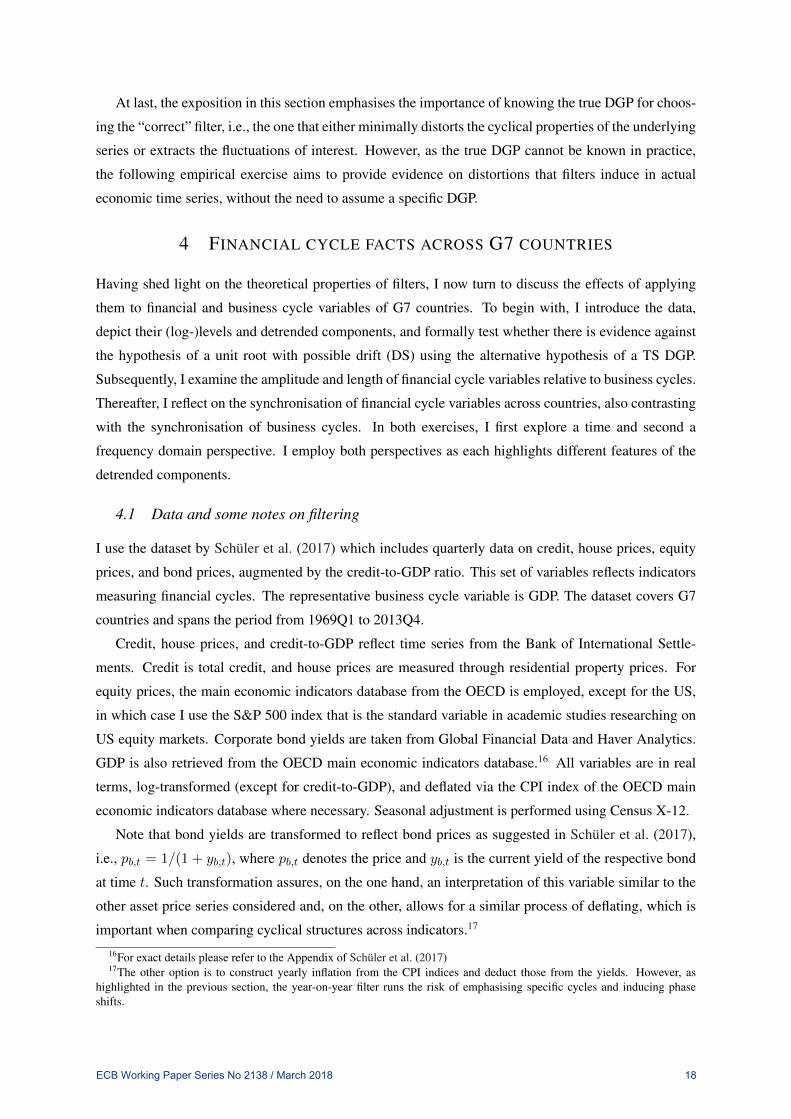
4.2.1 Time domain perspective
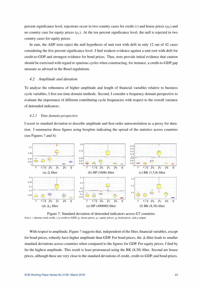
I resort to standard deviation to describe amplitude and first-order autocorrelation as a proxy for dura-
tion. I summarise these figures using boxplots indicating the spread of the statistics across countries
(see Figures 7 and 8).
c c/q ph pe pb q
(a) ∆ filter
c c/q ph pe pb q
(b) HP (1600) filter
c c/q ph pe pb q
(c) BK (1.5,8) filter
c c/q ph pe pb q
(d) ∆4 filter
c c/q ph pe pb q
(e) HP (400000) filter
c c/q ph pe pb q
(f) BK (8,30) filter
Figure 7: Standard deviation of detrended indicators across G7 countriesNotes: c denotes total credit, c/q credit-to-GDP, ph house prices, pe equity prices, pb bond prices, and q output.
With respect to amplitude, Figure 7 suggests that, independent of the filter, financial variables, except
for bond prices, robustly have higher amplitude than GDP. For bond prices, the ∆ filter leads to smaller
standard deviations across countries when compared to the figures for GDP. For equity prices, I find by
far the highest amplitude. This result is least pronounced using the BK (8,30) filter. Second are house
prices, although these are very close to the standard deviations of credit, credit-to-GDP, and bond prices.
ECB Working Paper Series No 2138 / March 2018 23
c c/q ph pe pb q
(a) ∆ filter
c c/q ph pe pb q
(b) HP (1600) filter
c c/q ph pe pb q
(c) BK (1.5,8) filter
c c/q ph pe pb q
(d) ∆4 filter
c c/q ph pe pb q
(e) HP (400000) filter
c c/q ph pe pb q
(f) BK (8,30) filter
Figure 8: First-order autocorrelation of detrended indicators across G7 countriesNotes: c denotes total credit, c/q credit-to-GDP, ph house prices, pe equity prices, pb bond prices, and q output. Note that scales differ forthe ∆ filter.
With respect to persistence, Figure 8 indicates that financial indicators, except for equity prices,
robustly have higher autocorrelation than GDP. Across detrending methods, it is not clear which variable
has the highest persistence. Lowest persistence is found for equity prices across methods of detrending,
except for the BK (8,30) filter, in which case output is least persistent.
Across filters and considering both amplitude and persistence, two results are worth noting. First,
differences to GDP appear to be rather marginal for HP (400000) and BK (8,30) filters; in the case of
persistence, also when considering the BK (1.5,8) filter. Second and in line with the first point, the
magnitude and dispersion of statistics vary strongly. Amplitude is highest for the HP (400000) filter,
while persistence is strongest for the BK (8,30) filter. These statistics are smallest for the ∆ filter. In
the case of persistence, for example, the range of the boxplots that describes the effects of the ∆ filter
stretches from around 0 to 0.9, while, at the other extreme, results of the BK (8,30) filter range from
close to 0.95 to around 1.
In sum, higher amplitude and persistence for credit, house prices, and bond prices as well as higher
amplitude of equity prices, all relative to GDP, are robust across the different methods of detrending.
Nonetheless, differences in the statistics are shown to be only marginally different for the HP (40000)
and the BK (8,30) filters – in the case of persistence, also for the BK (1.5,8) filter. In general, the
magnitude and dispersion of statistics across countries vary strongly across filters. These findings imply
that specific cycle frequencies of the stationary component are altered using the various filters and their
specifications.
4.2.2 Frequency domain perspective
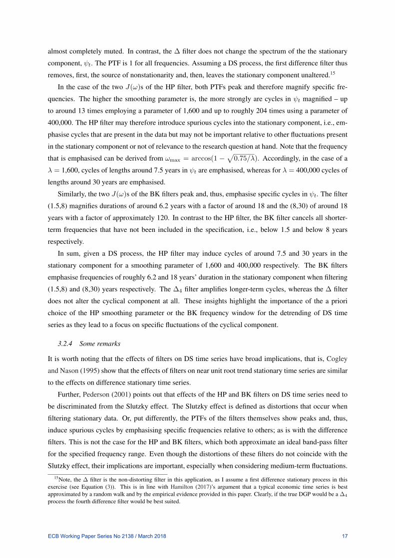
Figure 9 shows the estimated smoothed spectral densities for each detrended variable across countries.
The solid line reflects the median of all countries at given frequency ω, while the dashed lines denote the
25% and 75% quantiles. For each detrended variable, the estimated spectral density, Sξ(ω), is obtained
ECB Working Paper Series No 2138 / March 2018 24

∆fil
ter
∆4
filte
rH
P(1
600)
filte
rH
P(4
0000
0)fil
ter
BK
(1.5
,8)fi
lter
BK
(8,3
0)fil
ter
0/2
Radians
02
10-4
c
0/2
Radians
05
10-3
0/2
Radians
05
10-4
0/2
Radians
0
0.01
0.02
0/2
Radians
05
10-4
0/2
Radians
0
0.01
0.02
0/2
Radians
012
10-4
c/q
0/2
Radians
02
10-3
0/2
Radians
0
0.51
10-3
0/2
Radians
0
0.01
0/2
Radians
05
10-4
0/2
Radians
0
0.01
0.02
0/2
Radians
024
10-4
p h
0/2
Radians
05
10-3
0/2
Radians
02
10-3
0/2
Radians
0
0.02
0/2
Radians
012
10-3
0/2
Radians
0
0.02
0/2
Radians
02
10-3
p e
0/2
Radians
0
0.02
0.04
0/2
Radians
0
0.02
0/2
Radians
0
0.1
0/2
Radians
0
0.02
0/2
Radians
0
0.05
0.1
0/2
Radians
01
10-5
p b
0/2
Radians
0
0.005
0.01
0/2
Radians
05
10-4
0/2
Radians
0
0.01
0.02
0/2
Radians
05
10-4
0/2
Radians
0
0.01
0.02
0/2
Radians
05
10-5
q
0/2
Radians
05
10-4
0/2
Radians
02
10-4
0/2
Radians
012
10-3
0/2
Radians
024
10-4
0/2
Radians
01
10-3
Figu
re9:
Spec
tral
dens
ities
ofde
tren
ded
indi
cato
rsac
ross
G7
coun
trie
sN
otes
:T
hebl
uear
eam
arks
busi
ness
cycl
efr
eque
ncie
s(1
.5-8
year
s)an
dth
epu
rple
area
med
ium
-ter
mcy
cles
(8-3
0ye
ars)
.Sol
idlin
eis
med
ian
acro
ssco
untr
ies
atfr
eque
ncyω
;das
hed
lines
depi
ctth
e25
%an
d75
%qu
antil
es.
ECB Working Paper Series No 2138 / March 2018 25

using a Parzen window of length 4√T , where T denotes the sample size.21 Again, the blue area marks
1.5 to 8 years and the purple 8 to 30 years. Further, Table 2 reports the most important cycle length as
measured by the global maximum of each spectral density, i.e., for all combinations of filters, variables,
and countries.
Higher amplitude is supported by the frequency domain perspective (see Figure 9). That is, the
magnitude of spectral densities (y-axis) for all detrended financial variables is higher than that of GDP
(q), except for bond prices (bb) in the case of the ∆ filter.22
Visually, longer-duration financial cycles – except for equity prices – are only supported by the
difference filters. Here, financial variables are clearly marked by more important, i.e., with respect
to overall variance, medium-term cycles than GDP. The exception is the equity price series (pe) with
many important cycle frequencies located in the business cycle range, similar to GDP. Bond prices still
seem to be governed by a long-term trend, as most important cycles locate at the zero frequency, except
for the HP (1600) and BK (1.5,8) filters. Differences between the durations of financial and business
cycles seem to disappear when the HP and BK filters are considered. In that regard, Table 2 offers
a more detailed view: while for the difference filters longer-duration cycles in credit, credit-to-GDP,
and house prices to cycles in GDP are apparent (for example, looking at the ∆ filter and the median
values: 12.6/16.0/9.9 versus 5.9 years respectively), they are only marginally longer using the HP and
BK filters (e.g., HP (1600) filter and median values: 7.4/8.1/7.8 versus 6.2 years respectively). They are
even marginally shorter for house prices in the case of the HP (400000) filter and for credit-to-GDP in
the case of the BK (1.5,8) filter.
Looking across filters, there is strong evidence that the data generating process for most of the data
is DS, that is, there evidence of filter-induced cycles in the stationary component. First, the detrended
components of the HP and BK filters across all countries and variables have durations around frequen-
cies indicated by the PTFs under DS, i.e., close to 7.5/30 and 6.2/18 years (see Table 2). Note that, when
interpreting the similarities of durations of the HP (400000) and BK (8,30) filtered series, it is important
to keep in mind that the grid of cycle durations above eight years is very small. This becomes clear, for
instance, when comparing the size of the large blue shaded area (covering 5.5 years) with the size of
the small purple area (covering 22 years; see, for example, Figure 9). That is, even though differences
in years may appear large, the outcomes of the latter filters across countries can still be argued to be
very similar. Further and in the case of the HP (400000) filter, where deviations from the expected
cycle duration under DS are strongest, possibly stationary components do not contain cycles of exactly
30-year duration, thus, revealing other frequencies close to 30 years. These are amplified as well, albeit
to a smaller degree than cycles of 30 years. Finally, the ∆4-filtered series tend to show the distortions
present in case of a difference stationary process as well. For instance, in the case of credit-to-GDP, eq-
uity prices, and GDP, the ∆ filter suggests the presence of short-term cycles, which are not present using
the ∆4 filter (Figure 9). Moreover, long-term cycles are emphasised more than cycles in the business21Figures actually show pseudo spectra, meaning that the zero frequency is disregarded.22Note that to compare overall figures one would have to integrate the spectral densities for each detrended variable and
country. Thus, it is not entirely correct to compare the magnitude of important cycles across indicators. The time domainoffers an easier to interpret perspective in this case.
ECB Working Paper Series No 2138 / March 2018 26
Table 2: Cycle duration of detrended indicators
Variable ∆ ∆4 HP HP BK BK Variable ∆ ∆4 HP HP BK BKCountry (1600) (4·105) (1.5,8) (8,30) Country (1600) (4·105) (1.5,8) (8,30)
Credit (c) Equity prices (pe)Canada 12.3 12.3 8.9 14.6 6.5 14.9 Canada 3.5 3.5 6.9 10.2 6.2 13.6Germany ∞ ∞ 7.4 50.0 6.9 30.6 Germany 3.3 7.8 7.3 11.7 6.5 13.2France 11.8 11.9 7.0 13.7 5.9 14.9 France 3.1 7.0 6.8 22.3 6.3 17.8Italy 17.2 17.4 8.6 17.1 7.0 20.3 Italy 6.4 6.6 6.6 16.8 6.1 16.9Japan ∞ ∞ 6.4 ∞ 5.9 ∞ Japan 7.8 7.8 6.8 17.7 5.9 16.8UK 21.8 20.9 5.8 18.5 5.5 23.3 UK 5.8 6.3 6.3 23.8 5.9 21.8US 12.6 12.6 7.4 14.2 6.2 17.7 US 3.4 3.5 7.0 ∞ 6.4 23.5
Average 15.1 15.0 7.4 21.3 6.3 20.3 Average 4.8 6.1 6.8 17.1 6.2 17.7Median 12.6 12.6 7.4 15.8 6.2 19.0 Median 3.5 6.6 6.8 17.2 6.2 16.9
Credit-to-GDP (c/q) Bond prices (pb)Canada 11.4 11.4 8.7 14.0 5.4 14.3 Canada ∞ ∞ 7.1 ∞ 6.4 ∞Germany ∞ ∞ 3.8 24.1 4.4 23.0 Germany ∞ ∞ 8.1 14.1 6.3 16.4France 17.5 19.1 8.6 16.5 5.3 17.5 France ∞ ∞ 7.1 ∞ 6.3 ∞Italy ∞ ∞ 8.5 19.3 4.0 28.4 Italy ∞ ∞ 6.8 ∞ 6.2 ∞Japan ∞ ∞ 6.0 ∞ 5.7 ∞ Japan ∞ ∞ 6.5 36.6 5.5 23.5UK 18.0 17.1 8.1 16.8 5.6 24.1 UK ∞ ∞ 6.0 5.4 75.9US 14.4 14.3 7.6 15.4 6.4 20.9 US ∞ ∞ 6.5 81.9 5.7 ∞
Average 15.3 15.5 7.3 17.7 5.3 21.4 Average n.a. n.a. 6.9 44.2 6.0 38.6Median 16.0 15.7 8.1 16.7 5.4 22.0 Median n.a. n.a. 6.8 36.6 6.2 23.5
House prices (ph) GDP (q)Canada 12.6 12.6 7.0 15.1 6.5 15.6 Canada 13.9 14.0 6.2 16.1 5.8 15.3Germany 8.4 8.3 7.8 13.2 6.9 13.6 Germany ∞ ∞ 6.6 14.1 5.8 14.6France 15.2 15.2 9.5 16.3 5.7 16.8 France 0.9 5.7 5.9 15.6 5.7 15.1Italy 9.9 10.0 7.7 12.3 6.4 14.0 Italy ∞ ∞ 5.6 14.8 5.4 19.1Japan 9.2 8.9 7.8 ∞ 6.0 40.2 Japan ∞ ∞ 6.8 ∞ 6.0 21.6UK 9.4 10.1 6.7 14.8 5.9 16.7 UK 5.8 5.9 5.9 14.4 5.6 17.1US 11.4 11.6 8.0 14.9 6.2 15.1 US 6.0 6.2 6.3 15.2 6.0 ∞
Average 10.8 11.0 7.8 14.4 6.2 18.8 Average 6.7 7.9 6.2 15.1 5.8 17.1Median 9.9 10.1 7.8 14.9 6.2 15.6 Median 5.9 6.0 6.2 15.0 5.8 16.2
Duration of maximum amplified cycle under DS time series process- - 7.5 30.0 6.2 18.0 - - 7.5 30.0 6.2 18.0
Notes: Numbers indicate cycle length in years referring to global maximum of spectral density from 0 to π of the detrended componentobtained by the indicated filter. ∞ denotes that maximum cycle duration is global maximum of spectral density. Average and median arederived neglecting countries with cycle duration of∞.
cycle region. For instance, the three peaks in the financial and business cycle range of equity prices are
biased as though the underlying data was DS, i.e., amplifying the longer-duration cycles and relatively
dampening shorter-term ones. The same holds true for GDP and credit-to-GDP.
Second, the differences in variances of the detrended components (y-axis) across filters are broadly
in line with the distortions present with difference stationary data, implying that strongest biases of the
stationary component occur when extracting medium-term cycles (see Figure 9). Magnitudes are by
far the strongest for the HP (400000)- and BK (8,30)-filtered series, in which case the filters have an
amplification of cycles in the stationary component of a factor of around 204 for cycles close to 30 years
and 120 for cycles close to 18 years. For instance, the detrended credit-to-GDP ratio has a peak above
0.01 for both filters and the peak of the HP (400000)-detrended component is above the peak of the
BK (8,30)-filtered component. Second are the magnitudes of the ∆4 filtered series in which case the
filter has an amplification of cycles of a maximum factor of around 16 for longer-term cycles (peak of
credit-to-GDP above 0.002). The HP (1600) filter leads to values only slightly smaller than the ∆4 filter
(peak of credit-to-GDP above 0.0005), relating to the PTF in the DS case that shows a magnification
ECB Working Paper Series No 2138 / March 2018 27
of cycles of around 7.5 years by a factor of up to roughly 13. Interestingly, the BK (1.5,8) filter shows
magnitudes similar to the HP (1600) filter (peak of credit-to-GDP close to 0.0005), even though its PTF
in the DS case shows a magnification of up to 18 times, which is a stronger amplification than in the
case of the ∆4 filter. This can be reconciled by the fact that the ∆4 filter magnifies a greater range
of frequencies and does not sharply peak at a specific cycle duration. The smoothing of the spectral
densities in the estimation process can be argued to lead to such differences. The mentioned differences
in magnitudes across filters also hold true for bond prices, in which case, however, the ADF tests reject
the null hypothesis of unit root with drift in most cases. Bond prices, however, seem to be a special
case, as even after filtering they are governed by a long-term trend (except for the HP (1600) filter), thus
possibly neither being trend nor difference stationary.
In sum, the frequency domain perspective suggests two things: It supports higher amplitude and
longer-duration of financial cycles relative to business cycles for all methods of detrending and variables,
except for equity prices in the case of the difference filters. However, most important cycles of financial
variables reported using the HP and BK filters are, in nearly all cases, only marginally longer than cycles
in GDP. Second, there is strong evidence of spurious cycles for all HP- and BK-detrended series, since
each specification and filter leads to a similar-duration cycle that is line with the predicted duration of the
maximum amplified cycle under DS. Similar lengths of most important cycles across countries marks a
very strong result as different country histories, laws, and institutions should lead to different country
cycles, which are apparent using the difference filters. Note that, even though cycles of HP (1600)-
and BK (1.5,8)-detrended series have each similar durations, the potential bias for inference is still less
strong than considering HP (400000)- and BK (8,30)-detrended series, that is, while the former filters
still include fluctuations of other frequencies besides the maximum amplified frequency, the latter filters
– in relative terms – do not. Finally, the fourth difference filter eliminates all short run frequencies and
emphasises longer-term frequencies, which specifically matters for credit-to-GDP, equity prices, and
GDP.
4.3 Synchronisation of financial cycle variables across countries
Below I shed light on the synchronisation of financial cycle variables across G7 countries. First, I con-
sider a time domain perspective using average contemporaneous correlations for each detrended series
across countries and, second, I depict results from a frequency domain perspective. The frequency
domain analysis starts by introducing a measure I call dynamic power cohesion. This represents the
equivalent to the average contemporaneous correlation employed in the time domain, additionally al-
lowing to differentiate between the importance of common cycles, considering their relation to overall
variance of indicators and whether these common cycles contribute positively or negatively to the over-
all correlation.
4.3.1 Time domain perspective
For the analysis of synchronisation of variables across countries, I employ, as indicated, the standard
correlation measure between country pairs. These statistics are depicted in the boxplots of Figure 10,
ECB Working Paper Series No 2138 / March 2018 28

c c/q ph pe pb q
(a) ∆ filter
c c/q ph pe pb q
(b) HP (1600) filter
c c/q ph pe pb q
(c) BK (1.5,8) filter
c c/q ph pe pb q
(d) ∆4 filter
c c/q ph pe pb q
(e) HP (400000) filter
c c/q ph pe pb q
(f) BK (8,30) filter
Figure 10: Correlation of detrended indicators across G7 countriesNotes: c denotes total credit, c/q credit-to-GDP, ph house prices, pe equity prices, pb bond prices, and q output. BK filter uses K = 40.
showing their dispersion across countries. Each panel contains a comparison of correlations across
variables for one of the filters. The y-axis has been restricted for all panels and ranges from one to the
minimum value over all boxplots.
Equity and bond prices always belong to the variables that are most strongly synchronised across
countries. However, a clear difference to the synchronisation of GDP only exists when employing the
∆ filter – for bond prices also using the ∆4 filter. For the remaining filters and specifications, the
differences become more marginal or disappear. Differences are least marked when considering the
BK (1.5,8) filter. In this case, equity prices and GDP show a similar degree of synchronisation across
countries, caused by a strong increase in the synchronisation of GDP at these frequencies. Differences
to GDP are rather similar when considering the HP (1600) and the ∆4 filter. The HP (400000)- and
the BK (8,30)-filtered series show a strong increase in dispersion of country correlation, leading to a
vanishing of marked differences.
For credit, house prices, and credit-to-GDP results suggest a weaker (for example, looking at the
median) synchronisation than GDP across methods of detrending. However, the dispersion of statistics
is stronger than for GDP, thus leading to country cases that show a similar synchronisation to cycles in
GDP. While these results broadly hold for the difference filters and the HP (1600) and BK (1.5,8) filters,
they are distorted when considering the HP (400000) and BK (8,30) filters. Here, similar to the case of
equity and bond prices, the dispersion of statistics particularly increases, such that differences become
less clear. More severely, the filtered series show a strong negative correlation for some of the country
cycles, being strongest for credit-to-GDP, which, to this degree, is not apparent from any of the other
detrending procedures.
In sum, equity and bond prices belong to the variables that are most strongly synchronised, and
credit, credit-to-GDP, and house prices among the variables that are most weakly synchronised across
methods of detrending, in most cases being different from the synchronisation of GDP. Differences to
ECB Working Paper Series No 2138 / March 2018 29
the synchronisation of GDP turn marginal or disappear, e.g., for equity prices and bond prices when
using the BK (1.5,8) filter or for credit, credit-to-GDP, and house prices when considering medium-
term frequencies. The dispersion of synchronisation of cycles in credit, credit-to-GDP, and house prices
is largest, such that some country pairs are more strongly and some more weakly related. In that regard,
the application of the HP (400000) and BK (8,30) filters induces the greatest dispersion, resulting in
a strong negative correlation of cycles which, to this degree, is not apparent using any of the other
methods of detrending.
4.3.2 Frequency domain perspective
First, I introduce the methodology of dynamic power cohesion, subsequently, the method is used to shed
light on the synchronisation of financial cycle variables across G7 countries.
Methodology: Dynamic power cohesion – Are important common cycles positively or negativelyrelated?
The methodology developed in this section is based on work by Croux, Forni and Reichlin (2001) and
Schüler et al. (2015, 2017). Specifically, I combine, on the one hand, the idea of dynamic correlation
that indicates contemporaneous correlation over the frequency band and, on the other hand, power
cohesion that provides information about the common cycle frequencies that matter most with respect
to the overall variance of a set of indicators. Dynamic power cohesion can be argued to be the direct
correspondence of the previous exercise, just in the frequency domain. It allows to point out cycles
that account for the overall contemporaneous correlation measured in the last section. This highlights
whether the synchronisation of common cycles occurs at different frequencies using different filters,
also indicating whether cycles contribute positively or negatively to overall correlation.
As indicated, I call the proposed method dynamic power cohesion (DPCoh) and define it as
DPCohΞ(ω) =1
(M − 1)M
∑i6=j
cξiξj (ω)
σξiσξj, (25)
where 1 ≤ i ≤M , 1 ≤ j ≤M , Ξ = (Ξ′1, . . . ,Ξ′T )′ is a T×M matrix and Ξt = (ξ1,t, . . . , ξM,t) (1×
M ). Further, t = 1, . . . , T and M ≥ 2 reflect the time dimension and number of variables respectively,
and ω ∈ [−π, π] denotes the cycle frequency.23 Ξ is assumed to contain stationary stochastic processes
with well-defined normalised cross-spectral densities, where σξi and σξj are the standard deviations and
cξiξj (ω) is the co-spectrum of the detrended components ξi,t and ξj,t. The co-spectrum is defined as
the real part of the cross-spectrum, sξiξj (ω), which can be decomposed into the co-spectrum and the
quadrature-spectrum, qξiξj (ω), as
sξiξj (ω) = cξiξj (ω) + iqξiξj (ω). (26)
The co-spectrum measures the covariance in phase and the quadrature-spectrum out of phase.23Actually, considering the frequencies from 0 to π suffices to provide all information on cycles in phase, as only the real
part of the cross-spectral density is considered.
ECB Working Paper Series No 2138 / March 2018 30
To give some intuition on the proposed measure, note that integrating from −π to π yields the
correlations analysed in the previous section, i.e.,∫ π−π cξiξj (ω)dω
σξiσξj=
Cov[ξit, ξjt]
σξiσξj= ρξiξj (27)
The above identity has two implications: first, the co-spectrum may take positive as well as negative
values and, second, a positive co-spectrum at some frequency and negative at some other can potentially
cancel each other out when integrating to the overall covariance. For instance, Croux et al. (2001) show
that while a white noise process and its one-period lagged value have zero correlation, the co-spectrum
indicates perfect positive correlation in the long run (at frequency 0) and perfect negative in the short
run (at frequency π), overall, however, integrating to zero. Thus, dynamic correlation makes it possible
to gain more insights on the linear relation of two stationary processes than the standard correlation
measure.
Finally, note that dynamic power cohesion differs from cohesion based on dynamic correlation (see
Croux et al. (2001)) by relating the co-spectrum to the overall standard deviations and not the respective
auto-spectra at frequency ω. Thus, while dynamic correlation cohesion – as proposed by Croux et al.
(2001) – can be used to study linear similarities of two processes at each frequency ω, the suggested
measure provides information on the relative importance of frequencies with respect to the indicators’
overall fluctuations. For a further discussion – including a comparison to squared coherency – please
refer to Schüler et al. (2015, 2017).
Results
Dynamic power cohesion is depicted for all detrended series in Figure 11.24 The solid line reflects the
mean across countries at frequency ω, whereas the dashed lines represent the 25% and 75% quantiles.
The blue area marks the business cycle region, which is 1.5 to 8 years, and the purple marks the medium-
term cycle region of 8 to 30 years. The x-axis is restricted and shows the spectra from close to 0 to π/2,
i.e., one year is the shortest cycle length depicted. Note that, due to the normalisation of cross-spectral
densities (see Equation (25)), a comparison of the strength of synchronisation among indicators without
integrating over ω is difficult. Nonetheless, graphs serve to highlight differences in important cycle
frequencies that explain the synchronisation of detrended indicators across countries.
The correlation of indicators occurs at cycle frequencies that contribute strongly to the overall vari-
ance of the single detrended indicators (see Section 4.2.2). Thus, DPCoh suggests that synchronisation
of detrended series is based on filter-induced cycles in the case of the HP and BK filter, calling for
caution when analysing cross-country correlation. Emphasised cycles do not necessarily represent im-
portant fluctuations of the stationary component, i.e., with respect to its overall variance. Again, special
caution needs to be taken when extracting medium-term frequencies, as other cyclical components are
relatively more strongly muted than when considering the HP (1600) or BK (1.5,8) filters. For instance,
the HP (1600) and BK (1.5,8) detrended house prices still contain fluctuations in the business cycle24The cross-spectral densities used in the derivation of DPCoh are similarly obtained as the spectral densities, i.e., using a
Parzen window with length 4√T . Again, I show pseudo spectra, i.e., for which I exclude the zero frequency.
ECB Working Paper Series No 2138 / March 2018 31
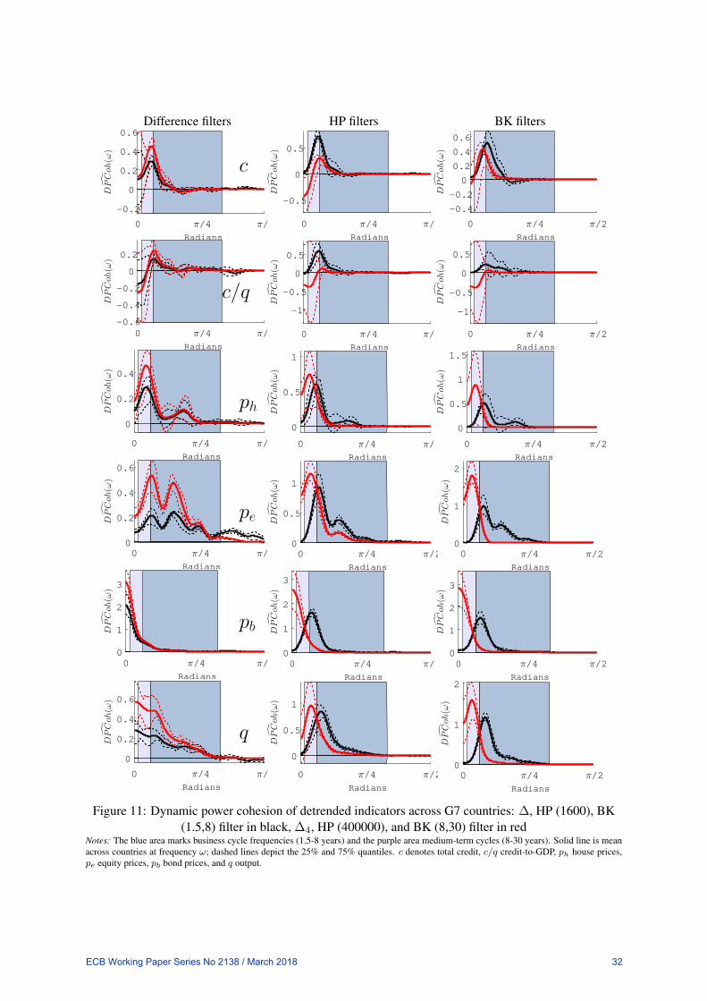
Difference filters HP filters BK filters
0 /4 /2
Radians
-0.2
0
0.2
0.4
0.6
c
0 /4 /2
Radians
-0.5
0
0.5
0 /4 /2
Radians
-0.4
-0.2
0
0.2
0.4
0.6
0 /4 /2
Radians
-0.6
-0.4
-0.2
0
0.2
c/q
0 /4 /2
Radians
-1
-0.5
0
0.5
0 /4 /2
Radians
-1
-0.5
0
0.5
0 /4 /2
Radians
0
0.2
0.4
ph
0 /4 /2
Radians
0
0.5
1
0 /4 /2
Radians
0
0.5
1
1.5
0 /4 /2
Radians
0
0.2
0.4
0.6
pe
0 /4 /2
Radians
0
0.5
1
0 /4 /2
Radians
0
1
2
0 /4 /2
Radians
0
1
2
3
pb
0 /4 /2
Radians
0
1
2
3
0 /4 /2
Radians
0
1
2
3
0 /4 /2
Radians
0
0.2
0.4
0.6
q
0 /4 /2
Radians
0
0.5
1
0 /4 /2
Radians
0
1
2
Figure 11: Dynamic power cohesion of detrended indicators across G7 countries: ∆, HP (1600), BK(1.5,8) filter in black, ∆4, HP (400000), and BK (8,30) filter in red
Notes: The blue area marks business cycle frequencies (1.5-8 years) and the purple area medium-term cycles (8-30 years). Solid line is meanacross countries at frequency ω; dashed lines depict the 25% and 75% quantiles. c denotes total credit, c/q credit-to-GDP, ph house prices,pe equity prices, pb bond prices, and q output.
ECB Working Paper Series No 2138 / March 2018 32

range, which are relatively muted considering the HP (400000) filter. Clearly, the BK (8,30) was spec-
ified to exclude frequencies below eight years, nonetheless, due to the amplification of medium-term
cycles, the HP (400000) detrended series contains similarly few important cycles in the business cycle
range.
Further, DPCoh suggests that the lower overall synchronisation of detrended credit and credit-to-
GDP is due to opposing medium-term cycles for certain country pairs, that is, the negative co-movement
at medium-term frequencies cancels out positive co-movement at shorter frequencies, such that overall
correlation is found to be lower than for GDP, e.g., for the ∆ filter. In general, for all filters, except the
HP (1600) filter, the range between the 75% and 25% quantile also reaches into the negative support
of the y-axis for medium-term cycles. In the case of the HP (1600) filter, these opposing medium-term
cycles are disregarded. In this light, previous results of strong negative correlation of HP (400000)- and
BK (8,30)-detrended series, e.g., of credit-to-GDP, can be explained by the amplification of medium-
term cycles that are negatively related for some country pairs and the relative dampening of shorter-term
fluctuations that are positively related.
Summarising, there is strong evidence that the synchronisation of HP- and BK-detrended series
occurs mostly at cycles induced by the filters, calling for caution in drawing inference from the latter.
Special attention needs to be taken when considering the medium term, as the amplification of such
cycles - in relative terms - strongly mutes shorter-term cycles, for instance, leading to strong negative
correlation of the HP (400000)- and BK (8,30)- detrended credit-to-GDP ratio. Finally, weaker overall
synchronisation of credit and credit-to-GDP is found to be due to opposing medium-term cycles.
5 CONCLUSIONS
Beyond enhancing financial system resilience, one of the key objectives of macroprudential policy is
to attenuate financial cycles. Clearly, central to this objective are the properties of financial variables.
These are of vital importance not only in terms of consistently informing policy makers and regulators,
but also in influencing the design of theoretical models. While I find that financial cycle properties
differ markedly across methods of detrending, their differences from similarly detrended GDP are qual-
itatively akin.
Nonetheless, caution needs to be exercised regarding the method of detrending, since I find sig-
nificant evidence of spurious cycles that bias inference, for instance, regarding the synchronisation of
detrended variables across countries. Specifically, a frequency domain perspective suggests that the
Hodrick and Prescott (1981, 1997) (HP) and Baxter and King (1999) (BK) filters, and, in general, any
band-pass filter amplify certain frequencies that lead to a relative dampening of other cycles, which
could be relevant for the research question or the specific policy task (see Section 2 for examples). The
negative consequences of spurious cycles increase for the HP filter in the magnitude of the smooth-
ing parameter and for the BK filter in the filtering of longer-term cycles, raising concerns about a HP
smoothing parameter of 400,000, as recommended in the Basel regulations or the smoothing window 8
to 30 years suggested by Drehmann et al. (2012).
ECB Working Paper Series No 2138 / March 2018 33

Further, I find evidence that the weak synchronisation of credit and credit-to-GDP across countries
(see Schüler et al. (2017)) is partially due to opposing medium-term cycles, which could potentially
relate to differing degrees of financial market liberalisation (see Favilukis et al. (2013)).
Three main policy conclusions may be drawn from this study. First, caution needs to be exercised
when analysing extracted medium-term cycles, as for instance suggested in Basel III. The strong am-
plification of a small range of cycles cancels shorter-term frequencies that could be potentially relevant,
say, in signalling the build-up of imbalances prior to systemic banking crises or the abrupt risk materi-
alisation thereafter. Also, if the frequency of financial crises increases, build-up phases of imbalances
will not be visible when focussing exclusively on a very specific medium-term frequency range. Hence,
there is a high risk that the recommended credit-to-GDP gap will misguide the setting of the CCyB
rate. Second, assuming the same HP smoothing parameter or BK frequency window across different
countries, means that relevant country-specific fluctuations are likely to be missed. While the US Basel
credit-to-GDP gap indicates imbalances before the savings and loan crisis and the global financial cri-
sis, the emphasis of such medium-term frequencies does not necessarily imply that Basel credit-to-GDP
gaps signal systemic banking crises for other countries as well – rather the opposite: the strong ampli-
fication of medium-term cycles is prone to miss fluctuations of relevance for other countries. The same
argument also holds for studies researching on business cycles that assume similar detrending specifi-
cations across countries; however, the risk of missing relevant fluctuations is greater when considering
medium-term cycles. Third, differing empirical properties of financial and business cycle variables
make a strong case for macroprudential policy possibly taking a complementary role to other macroe-
conomic policies that primarily target business cycles.
Two avenues for addressing the risks of spurious cycles seem reasonable: First, one could com-
pletely avoid the application of HP and BK filters on trending levels by considering their growth rates.
Of course, stationary growth rates could still be filtered to focus on specific frequencies. In this re-
gard, Schüler et al. (2015, 2017) suggest forming cross-sectional averages (with time-varying weights)
of standardised growth rates of credit and asset prices which allow to focus on expansions and con-
tractions common to this set of variables, thus dampening idiosyncratic movements. Such measure
already provides a relatively smooth estimate of cyclical fluctuations without the need to rely on further
filtering techniques. The authors show in a real-time early warning exercise that a filtered composite
financial cycle – by far – outperforms the credit-to-GDP gap for G7 countries, possibly reflecting the
fact that the large HP smoothing parameter emphasises frequencies that are not relevant in some country
cases. Second, one could still rely on HP and BK filters for detrending, albeit using country-specific HP
smoothing parameters or frequency windows (possibly changing over time) that amplify frequencies
relevant for the specific task. In this context, Schüler et al. (2015, 2017) propose a methodology for
forming country-specific cycle frequencies that are based on the cohesion, i.e., correlation, between the
growth rates of financial cycle indicators in the frequency domain. Alternatively, one could use unob-
served components models that lead to country-specific cycles (see, for example, Rünstler and Vlekke
(2016); Galati et al. (2016)). However, for this class of models, too, studies find evidence of spurious
cycles if the true DGP is DS (Nelson (1988)).
ECB Working Paper Series No 2138 / March 2018 34
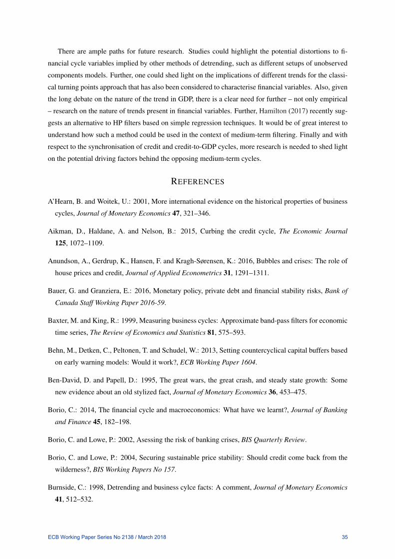
There are ample paths for future research. Studies could highlight the potential distortions to fi-
nancial cycle variables implied by other methods of detrending, such as different setups of unobserved
components models. Further, one could shed light on the implications of different trends for the classi-
cal turning points approach that has also been considered to characterise financial variables. Also, given
the long debate on the nature of the trend in GDP, there is a clear need for further – not only empirical
– research on the nature of trends present in financial variables. Further, Hamilton (2017) recently sug-
gests an alternative to HP filters based on simple regression techniques. It would be of great interest to
understand how such a method could be used in the context of medium-term filtering. Finally and with
respect to the synchronisation of credit and credit-to-GDP cycles, more research is needed to shed light
on the potential driving factors behind the opposing medium-term cycles.
REFERENCES
A’Hearn, B. and Woitek, U.: 2001, More international evidence on the historical properties of business
cycles, Journal of Monetary Economics 47, 321–346.
Aikman, D., Haldane, A. and Nelson, B.: 2015, Curbing the credit cycle, The Economic Journal
125, 1072–1109.
Anundson, A., Gerdrup, K., Hansen, F. and Kragh-Sørensen, K.: 2016, Bubbles and crises: The role of
house prices and credit, Journal of Applied Econometrics 31, 1291–1311.
Bauer, G. and Granziera, E.: 2016, Monetary policy, private debt and financial stability risks, Bank of
Canada Staff Working Paper 2016-59.
Baxter, M. and King, R.: 1999, Measuring business cycles: Approximate band-pass filters for economic
time series, The Review of Economics and Statistics 81, 575–593.
Behn, M., Detken, C., Peltonen, T. and Schudel, W.: 2013, Setting countercyclical capital buffers based
on early warning models: Would it work?, ECB Working Paper 1604.
Ben-David, D. and Papell, D.: 1995, The great wars, the great crash, and steady state growth: Some
new evidence about an old stylized fact, Journal of Monetary Economics 36, 453–475.
Borio, C.: 2014, The financial cycle and macroeconomics: What have we learnt?, Journal of Banking
and Finance 45, 182–198.
Borio, C. and Lowe, P.: 2002, Asessing the risk of banking crises, BIS Quarterly Review.
Borio, C. and Lowe, P.: 2004, Securing sustainable price stability: Should credit come back from the
wilderness?, BIS Working Papers No 157.
Burnside, C.: 1998, Detrending and business cylce facts: A comment, Journal of Monetary Economics
41, 512–532.
ECB Working Paper Series No 2138 / March 2018 35

Canova, F.: 1998a, Detrending and business cycle facts, Journal of Monetary Economics 41, 475–512.
Canova, F.: 1998b, Detrending and business cycle facts: A user’s guide, Journal of Monetary Economics
41, 533–540.
Cheung, Y.-W. and Chinn, M.: 1997, Further investigation of the uncertain unit root in GNP, Journal of
Business and Economic Statistics 15, 68–73.
Christiano, L. and Fitzgerald, T.: 2003, The band pass filter, International Economic Review 44, 435–
465.
Claessens, S., Kose, M. and Terrones, M.: 2011, Financial cycles: What? How? When?, IMF Working
Paper WP/11/76.
Claessens, S., Kose, M. and Terrones, M.: 2012, How do business and financial cycles interact?, Journal
of International Economics 87, 178–190.
Cogley, T. and Nason, J.: 1995, Effects of the Hodrick-Prescott filter on trend and difference stationary
time series. Implications for business cycle research, Journal of Economic Dynamics and Control
19, 253–278.
Croux, C., Forni, M. and Reichlin, L.: 2001, A measure of comovement for economic variables: Theory
and empirics, The Review of Economics and Statistics 83, 232–241.
Darne, O. and Dieboldt, C.: 2004, Unit roots and infrequent large shocks: New international evidence
on ouput, Journal of Monetary Economics 51, 1449–1465.
Diebold, F. and Senhadji, A.: 1996, The uncertain root in real GNP: Comment, American Economic
Review 86, 1291–1298.
Drehmann, M., Borio, C. and Tsatsaronis, K.: 2012, Characterising the financial cycle: Don’t lose sight
of the medium term!, BIS Working Paper 380.
European Central Bank: 2009, The concept of systemic risk, Financial Stability Review, Special Feature
B, December.
Favilukis, L., Kohn, D., Ludvigson, S. and Van Nieuwerburgh, S.: 2013, International capital flows
and house prices: Theory and evidence, in E. Glaeser and T. Sinai (eds), Housing and the Financial
Crisis, University of Chicago Press, Chicago, pp. 235–299.
Galati, G., Hindrayanto, I., Koopman, S. and Vlekke, M.: 2016, Measuring financial cycles with a
model-based filter: Empirical evidence for the United States and the euro area, Economics Letters
145, 83–87.
Granger, C.: 1966, The typical spectral shape of an economic variable, Econometrica 34, 150–161.
ECB Working Paper Series No 2138 / March 2018 36

Hall, A.: 1994, Testing for a unit root in time series with pretest data-based model selection, Journal of
Business and Economics Statistics 12, 461–470.
Hamilton, J.: 2017, Why you should never use the Hodrick-Prescott filter, The Review of Economics
and Statistics: Just Accepted MS.
Harding, D. and Pagan, A.: 2005, A suggested framework for classifying the modes of cycle research,
Journal of Applied Econometrics 20, 151–159.
Harvey, A. and Jaeger, A.: 1993, Detrending, stylized facts and the busines cycle, Journal of Applied
Econometrics 8, 231–247.
Hiebert, P., Klaus, B., Peltonen, T., Schüler, Y. and Welz, P.: 2014, Capturing the financial cycle in the
euro area, Financial Stability Review: Special Feature B.
Hodrick, R. and Prescott, E.: 1981, Postwar U.S. business cycles: An empirical investigation, Discus-
sion Paper 451, Northwestern University.
Hodrick, R. and Prescott, E.: 1997, Postwar U.S. business cycles: An empirical investigation, Journal
of Money, Credit and Banking 29, 1–16.
Jordà, O., Schularick, M. and Taylor, A. M.: 2017, Macrofinancial History and the New Business
Cycle Facts, in M. Eichenbaum and J. Parker (eds), NBER Macroeconomics Annual 2016, Volume
31, University of Chicago Press, Chicago, chapter 3, pp. 213–263.
King, R. and Rebelo, S.: 1993, Low frequency filtering and real business cycles, Journal of Economic
Dynamics and Control 17, 207–231.
Laeven, L. and Valencia, F.: 2012, Systemic banking crises database: An update, IMF Working Paper
WP/12/163.
Meller, B. and Metiu, N.: 2015, The synchronization of European credit cycles, Deutsche Bundesbank
Discussion Paper 20/2015.
Meller, B. and Metiu, N.: forthcoming, The synchronization of credit cycles, Journal of Banking and
Finance.
Murray, C.: 2003, Cyclical properties of Baxter-King filtered time series, The Review of Economics and
Statistics 85, 472–476.
Murray, C. and Nelson, C.: 2000, The uncertain trend in U.S. GDP, Journal of Monetary Economics
46, 79–95.
Nelson, C.: 1988, Spurious trends and cycle in the state space decomposition of a time series with a
unit root, Journal of Economic Dynamics and Control 12, 475–488.
ECB Working Paper Series No 2138 / March 2018 37

Nelson, C. and Plosser, C.: 1982, Trends and random walks in macroeconomic time series. Some
evidence and implications, Journal of Monetary Economics 10, 139–162.
Pederson, T.: 2001, The Hodrick-Prescott filter, the Slutzky effect, and the distortionary effects of filters,
Journal of Economic Dynamics and Contril 25, 1081–1101.
Perron, P.: 1989, The great crash, the oil price shock, and the unit root hypothesis, Econometrica
57, 1361–1401.
Rünstler, G. and Vlekke, M.: 2016, Business, housing and credit cycles, ECB Working Paper 1915.
Schularick, M. and Taylor, A.: 2012, Credit booms gone bust: Monetary policy, leverage cycles, and
financial crises, 1870-2008, American Economic Review 102, 1029–1061.
Schüler, Y., Hiebert, P. and Peltonen, T.: 2015, Characterising the financial cycle: A multivariate and
time-varying approach, ECB Working Paper 1846.
Schüler, Y., Hiebert, P. and Peltonen, T.: 2017, Coherent financial cycles for G-7 countries: Why
extending credit can be an asset, ESRB Working Paper Series No. 43.
Schwarz, G.: 1978, Estimating the dimension of a model, The Annals of Statistics 6, 461–464.
Stremmel, H.: 2015, Capturing the financial cycle in Europe, ECB Working Paper 1811.
Strohsal, T., Proaño, C. and Wolters, J.: 2015a, Characterizing the financial cycle: Evidence from a
frequency domain analysis, Deutsche Bundesbank Discussion Paper 22/2015.
Strohsal, T., Proaño, C. and Wolters, J.: 2015b, How do financial cycles interact? Evidence for the US
and the UK, SFB 649 Discussion Paper 2015-024.
Verona, F.: 2016, Time-frequency characterization of the U.S. financial cycle, Economics Letters
144, 75–79.
Vougas, D.: 2007, Is the trend in post-WW II US real GDP uncertain or non-linear?, Economics Letters
94, 348–355.
Zivot, E. and Andrews, D.: 1992, Further evidence on the great crash, the oil-price shock, and the unit
root hypothesis, Journal of Business and Economics Statistics 10, 251–270.
ECB Working Paper Series No 2138 / March 2018 38
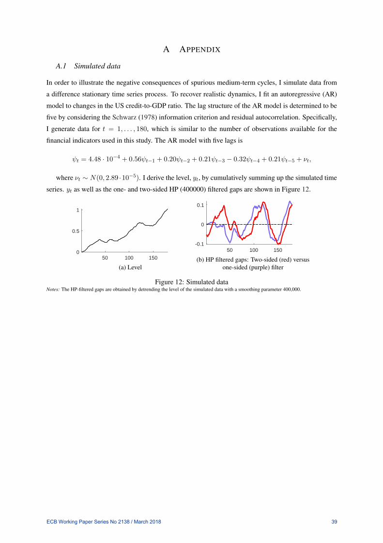
A APPENDIX
A.1 Simulated data
In order to illustrate the negative consequences of spurious medium-term cycles, I simulate data from
a difference stationary time series process. To recover realistic dynamics, I fit an autoregressive (AR)
model to changes in the US credit-to-GDP ratio. The lag structure of the AR model is determined to be
five by considering the Schwarz (1978) information criterion and residual autocorrelation. Specifically,
I generate data for t = 1, . . . , 180, which is similar to the number of observations available for the
financial indicators used in this study. The AR model with five lags is
ψt = 4.48 · 10−4 + 0.56ψt−1 + 0.20ψt−2 + 0.21ψt−3 − 0.32ψt−4 + 0.21ψt−5 + νt,
where νt ∼ N(0, 2.89 ·10−5). I derive the level, yt, by cumulatively summing up the simulated time
series. yt as well as the one- and two-sided HP (400000) filtered gaps are shown in Figure 12.
50 100 1500
0.5
1
(a) Level
50 100 150-0.1
0
0.1
(b) HP filtered gaps: Two-sided (red) versusone-sided (purple) filter
Figure 12: Simulated dataNotes: The HP-filtered gaps are obtained by detrending the level of the simulated data with a smoothing parameter 400,000.
ECB Working Paper Series No 2138 / March 2018 39
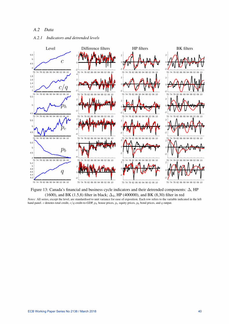
A.2 Data
A.2.1 Indicators and detrended levels
Level Difference filters HP filters BK filters
70 74 78 82 86 90 94 98 02 06 10
4
4.5
5
5.5
c
70 74 78 82 86 90 94 98 02 06 10-2
0
2
70 74 78 82 86 90 94 98 02 06 10
-2
0
2
70 74 78 82 86 90 94 98 02 06 10
-2
0
2
70 74 78 82 86 90 94 98 02 06 10
1
1.2
1.4
1.6
1.8
c/q70 74 78 82 86 90 94 98 02 06 10
-2
0
2
4
70 74 78 82 86 90 94 98 02 06 10
-2
0
2
70 74 78 82 86 90 94 98 02 06 10-2
0
2
70 74 78 82 86 90 94 98 02 06 104.5
5
5.5
ph
70 74 78 82 86 90 94 98 02 06 10
-2
0
2
70 74 78 82 86 90 94 98 02 06 10
-2
0
2
70 74 78 82 86 90 94 98 02 06 10
-2
0
2
70 74 78 82 86 90 94 98 02 06 10
4.5
5
5.5
pe
70 74 78 82 86 90 94 98 02 06 10
-4
-2
0
2
70 74 78 82 86 90 94 98 02 06 10
-2
0
2
70 74 78 82 86 90 94 98 02 06 10
-2
0
2
70 74 78 82 86 90 94 98 02 06 104
4.5
5
5.5
pb
70 74 78 82 86 90 94 98 02 06 10
-4
-2
0
70 74 78 82 86 90 94 98 02 06 10
-2
0
2
70 74 78 82 86 90 94 98 02 06 10
-2
0
2
70 74 78 82 86 90 94 98 02 06 10
4.24.44.64.8
55.2
q
70 74 78 82 86 90 94 98 02 06 10
-2
0
2
70 74 78 82 86 90 94 98 02 06 10
-2
0
2
70 74 78 82 86 90 94 98 02 06 10
-2
0
2
Figure 13: Canada’s financial and business cycle indicators and their detrended components: ∆, HP(1600), and BK (1.5,8) filter in black; ∆4, HP (400000), and BK (8,30) filter in red
Notes: All series, except the level, are standardised to unit variance for ease of exposition. Each row refers to the variable indicated in the lefthand panel. c denotes total credit, c/q credit-to-GDP, ph house prices, pe equity prices, pb bond prices, and q output.
ECB Working Paper Series No 2138 / March 2018 40
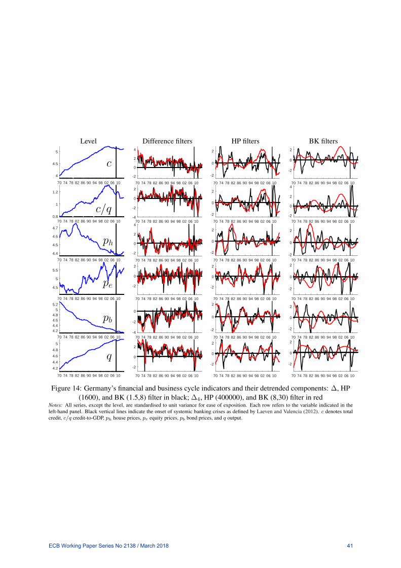
Level Difference filters HP filters BK filters
70 74 78 82 86 90 94 98 02 06 10
4
4.5
5
c
70 74 78 82 86 90 94 98 02 06 10
-2
0
2
4
70 74 78 82 86 90 94 98 02 06 10
-2
0
2
70 74 78 82 86 90 94 98 02 06 10
-2
0
2
70 74 78 82 86 90 94 98 02 06 100.8
1
1.2
c/q70 74 78 82 86 90 94 98 02 06 10
-4
-2
0
2
70 74 78 82 86 90 94 98 02 06 10
-2
0
2
70 74 78 82 86 90 94 98 02 06 10
-2
0
2
4
70 74 78 82 86 90 94 98 02 06 10
4.4
4.5
4.6
4.7
ph
70 74 78 82 86 90 94 98 02 06 10
-2
0
2
4
70 74 78 82 86 90 94 98 02 06 10
-2
0
2
70 74 78 82 86 90 94 98 02 06 10-2
0
2
70 74 78 82 86 90 94 98 02 06 10
4.5
5
5.5
pe70 74 78 82 86 90 94 98 02 06 10
-2
0
2
70 74 78 82 86 90 94 98 02 06 10
-2
0
2
70 74 78 82 86 90 94 98 02 06 10
-2
0
2
70 74 78 82 86 90 94 98 02 06 10
4.24.44.64.8
55.2
pb
70 74 78 82 86 90 94 98 02 06 10-4
-2
0
70 74 78 82 86 90 94 98 02 06 10
-2
0
2
70 74 78 82 86 90 94 98 02 06 10
-2
0
2
70 74 78 82 86 90 94 98 02 06 10
4.2
4.4
4.6
4.8
5
q
70 74 78 82 86 90 94 98 02 06 10
-2
0
2
70 74 78 82 86 90 94 98 02 06 10
-2
0
2
70 74 78 82 86 90 94 98 02 06 10
-2
0
2
Figure 14: Germany’s financial and business cycle indicators and their detrended components: ∆, HP(1600), and BK (1.5,8) filter in black; ∆4, HP (400000), and BK (8,30) filter in red
Notes: All series, except the level, are standardised to unit variance for ease of exposition. Each row refers to the variable indicated in theleft-hand panel. Black vertical lines indicate the onset of systemic banking crises as defined by Laeven and Valencia (2012). c denotes totalcredit, c/q credit-to-GDP, ph house prices, pe equity prices, pb bond prices, and q output.
ECB Working Paper Series No 2138 / March 2018 41

Level Difference filters HP filters BK filters
70 74 78 82 86 90 94 98 02 06 104
4.5
5
5.5
c
70 74 78 82 86 90 94 98 02 06 10
0
2
4
70 74 78 82 86 90 94 98 02 06 10
-2
0
2
70 74 78 82 86 90 94 98 02 06 10
-2
0
2
70 74 78 82 86 90 94 98 02 06 10
1
1.2
1.4
1.6
c/q70 74 78 82 86 90 94 98 02 06 10
-1
0
1
2
3
70 74 78 82 86 90 94 98 02 06 10
-2
0
2
70 74 78 82 86 90 94 98 02 06 10-2
0
2
70 74 78 82 86 90 94 98 02 06 10
4.6
4.8
5
5.2
5.4
ph70 74 78 82 86 90 94 98 02 06 10
-2
0
2
70 74 78 82 86 90 94 98 02 06 10
-2
0
2
70 74 78 82 86 90 94 98 02 06 10
-2
0
2
70 74 78 82 86 90 94 98 02 06 10
4.5
5
5.5
6
pe
70 74 78 82 86 90 94 98 02 06 10
-2
0
2
70 74 78 82 86 90 94 98 02 06 10
-2
0
2
70 74 78 82 86 90 94 98 02 06 10
-2
0
2
70 74 78 82 86 90 94 98 02 06 10
4.5
5
5.5
6
pb
70 74 78 82 86 90 94 98 02 06 10
-4
-2
0
70 74 78 82 86 90 94 98 02 06 10
-2
0
2
70 74 78 82 86 90 94 98 02 06 10
-2
0
2
70 74 78 82 86 90 94 98 02 06 104.2
4.4
4.6
4.8
5
q
70 74 78 82 86 90 94 98 02 06 10
-4
-2
0
2
70 74 78 82 86 90 94 98 02 06 10
-2
0
2
70 74 78 82 86 90 94 98 02 06 10
-2
0
2
Figure 15: France’s financial and business cycle indicators and their detrended components: ∆, HP(1600), and BK (1.5,8) filter in black; ∆4, HP (400000), and BK (8,30) filter in red
Notes: All series, except the level, are standardised to unit variance for ease of exposition. Each row refers to the variable indicated in theleft-hand panel. Black vertical lines indicate the onset of systemic banking crises as defined by Laeven and Valencia (2012). c denotes totalcredit, c/q credit-to-GDP, ph house prices, pe equity prices, pb bond prices, and q output.
ECB Working Paper Series No 2138 / March 2018 42

Level Difference filters HP filters BK filters
70 74 78 82 86 90 94 98 02 06 10
4.5
5
5.5
c
70 74 78 82 86 90 94 98 02 06 10
-2
0
2
70 74 78 82 86 90 94 98 02 06 10-2
0
2
70 74 78 82 86 90 94 98 02 06 10
-2
0
2
70 74 78 82 86 90 94 98 02 06 10
0.6
0.8
1
1.2
c/q
70 74 78 82 86 90 94 98 02 06 10
-2
0
2
70 74 78 82 86 90 94 98 02 06 10
-1
0
1
2
70 74 78 82 86 90 94 98 02 06 10-2
0
2
70 74 78 82 86 90 94 98 02 06 10
4.4
4.6
4.8
5
5.2
ph
70 74 78 82 86 90 94 98 02 06 10
0
2
4
70 74 78 82 86 90 94 98 02 06 10
-2
0
2
70 74 78 82 86 90 94 98 02 06 10
-2
0
2
70 74 78 82 86 90 94 98 02 06 10
4
5
6
pe70 74 78 82 86 90 94 98 02 06 10
-2
0
2
70 74 78 82 86 90 94 98 02 06 10-2
0
2
70 74 78 82 86 90 94 98 02 06 10-2
0
2
70 74 78 82 86 90 94 98 02 06 10
4
5
6
pb
70 74 78 82 86 90 94 98 02 06 10
-4
-2
0
70 74 78 82 86 90 94 98 02 06 10
-2
0
2
70 74 78 82 86 90 94 98 02 06 10
-2
0
2
70 74 78 82 86 90 94 98 02 06 10
4.2
4.4
4.6
4.8
5
q
70 74 78 82 86 90 94 98 02 06 10
-2
0
2
4
70 74 78 82 86 90 94 98 02 06 10
-2
0
2
70 74 78 82 86 90 94 98 02 06 10
-2
0
2
Figure 16: Italy’s financial and business cycle indicators and their detrended components: ∆, HP(1600), and BK (1.5,8) filter in black; ∆4, HP (400000), and BK (8,30) filter in red
Notes: All series, except the level, are standardised to unit variance for ease of exposition. Each row refers to the variable indicated in the lefthand panel. Black vertical lines indicate the onset of systemic banking crises as defined by Laeven and Valencia (2012). c denotes total credit,c/q credit-to-GDP, ph house prices, pe equity prices, pb bond prices, and q output.
ECB Working Paper Series No 2138 / March 2018 43

Level Difference filters HP filters BK filters
70 74 78 82 86 90 94 98 02 06 10
4
4.5
5
c
70 74 78 82 86 90 94 98 02 06 10
-2
0
2
70 74 78 82 86 90 94 98 02 06 10-2
0
2
4
70 74 78 82 86 90 94 98 02 06 10
-2
0
2
70 74 78 82 86 90 94 98 02 06 10
1.4
1.6
1.8
2
2.2
c/q70 74 78 82 86 90 94 98 02 06 10
-2
0
2
4
70 74 78 82 86 90 94 98 02 06 10
-2
0
2
70 74 78 82 86 90 94 98 02 06 10
-2
0
2
70 74 78 82 86 90 94 98 02 06 10
4.4
4.6
4.8
ph
70 74 78 82 86 90 94 98 02 06 10
-2
0
2
4
70 74 78 82 86 90 94 98 02 06 10
0
2
4
70 74 78 82 86 90 94 98 02 06 10
0
2
4
70 74 78 82 86 90 94 98 02 06 10
4
4.5
5
5.5
pe70 74 78 82 86 90 94 98 02 06 10
-4
-2
0
2
70 74 78 82 86 90 94 98 02 06 10-2
0
2
70 74 78 82 86 90 94 98 02 06 10
-1
0
1
2
70 74 78 82 86 90 94 98 02 06 104.5
5
5.5
pb
70 74 78 82 86 90 94 98 02 06 10
-6
-4
-2
0
70 74 78 82 86 90 94 98 02 06 10
-2
0
2
4
70 74 78 82 86 90 94 98 02 06 10
-2
0
2
70 74 78 82 86 90 94 98 02 06 10
4
4.5
5
q
70 74 78 82 86 90 94 98 02 06 10
-2
0
2
70 74 78 82 86 90 94 98 02 06 10
-2
0
2
70 74 78 82 86 90 94 98 02 06 10
-2
0
2
Figure 17: Japan’s financial and business cycle indicators and their detrended components: ∆, HP(1600), and BK (1.5,8) filter in black; ∆4, HP (400000), and BK (8,30) filter in red
Notes: All series, except the level, are standardised to unit variance for ease of exposition. Each row refers to the variable indicated in theleft-hand panel. Black vertical lines indicate the onset of systemic banking crises as defined by Laeven and Valencia (2012). c denotes totalcredit, c/q credit-to-GDP, ph house prices, pe equity prices, pb bond prices, and q output.
ECB Working Paper Series No 2138 / March 2018 44

Level Difference filters HP filters BK filters
70 74 78 82 86 90 94 98 02 06 104
5
6
c
70 74 78 82 86 90 94 98 02 06 10
-2
0
2
70 74 78 82 86 90 94 98 02 06 10
-2
0
2
70 74 78 82 86 90 94 98 02 06 10
-2
0
2
70 74 78 82 86 90 94 98 02 06 100.60.8
11.21.41.61.8
c/q70 74 78 82 86 90 94 98 02 06 10
-2
0
2
4
70 74 78 82 86 90 94 98 02 06 10
-2
0
2
70 74 78 82 86 90 94 98 02 06 10-2
0
2
70 74 78 82 86 90 94 98 02 06 10
4.5
5
5.5
ph
70 74 78 82 86 90 94 98 02 06 10-2
0
2
70 74 78 82 86 90 94 98 02 06 10-2
0
2
70 74 78 82 86 90 94 98 02 06 10
-2
0
2
70 74 78 82 86 90 94 98 02 06 10
4
4.5
5
5.5
pe
70 74 78 82 86 90 94 98 02 06 10
-4
-2
0
2
70 74 78 82 86 90 94 98 02 06 10
-4
-2
0
2
70 74 78 82 86 90 94 98 02 06 10
-2
0
2
70 74 78 82 86 90 94 98 02 06 10
4
5
6
pb
70 74 78 82 86 90 94 98 02 06 10
-4
-2
0
70 74 78 82 86 90 94 98 02 06 10
-2
0
2
70 74 78 82 86 90 94 98 02 06 10
-2
0
2
70 74 78 82 86 90 94 98 02 06 10
4.4
4.6
4.8
5
5.2
q
70 74 78 82 86 90 94 98 02 06 10
-2
0
2
4
70 74 78 82 86 90 94 98 02 06 10
-2
0
2
70 74 78 82 86 90 94 98 02 06 10
-2
0
2
Figure 18: UK’s financial and business cycle indicators and their detrended components: ∆, HP(1600), and BK (1.5,8) filter in black; ∆4, HP (400000), and BK (8,30) filter in red
Notes: All series, except the level, are standardised to unit variance for ease of exposition. Each row refers to the variable indicated in theleft-hand panel. Black vertical lines indicate the onset of systemic banking crises as defined by Laeven and Valencia (2012). c denotes totalcredit, c/q credit-to-GDP, ph house prices, pe equity prices, pb bond prices, and q output.
ECB Working Paper Series No 2138 / March 2018 45

A.2.2 Credit-to-GDP gap: Two-sided versus one-sided HP filter
70 74 78 82 86 90 94 98 02 06 10
-2
0
2
(a) Canada
70 74 78 82 86 90 94 98 02 06 10
-2
0
2
(b) Germany
70 74 78 82 86 90 94 98 02 06 10
-1
0
1
2
(c) France
70 74 78 82 86 90 94 98 02 06 10
-1
0
1
2
(d) Italy
70 74 78 82 86 90 94 98 02 06 10
-2
-1
0
1
(e) Japan
70 74 78 82 86 90 94 98 02 06 10
-2
0
2
(f) UK
70 74 78 82 86 90 94 98 02 06 10
-2
0
2
(g) US
Figure 19: Credit-to-GDP gap: Two-sided (red) versus one-sided (purple) HP filterNotes: Black vertical lines indicate the onset of systemic banking crises as defined by Laeven and Valencia (2012). All series are standardisedto unit variance for ease of exposition.
ECB Working Paper Series No 2138 / March 2018 46

Acknowledgements I would like to thank Klaus Adam, Geert Bekaert, Claudia Foroni, James Hamilton, Lutz Kilian, Fabian Krüger, Petros M. Migiakis, Emanuel Mönch, Gerhard Rünstler, Bernd Schwaab, Lars Svensson, Jesus Fernandez-Villaverde, Mark Watson, and Kenneth West for helpful discussions. Further, I would like to thank the audience at the CFE 2016, 1st Annual Workshop of the ESCB Research Cluster 3, and the Bundesbank Research Seminar, as well as an anonymous referee for their valuable comments and suggestions. Annika Bacher provided outstanding research assistance. The views expressed in this paper are those of the author and do not necessarily coincide with the views of the Deutsche Bundesbank, the European Central Bank, or the Eurosystem. Any errors are the responsibility of the author.
Yves S. Schüler Deutsche Bundesbank and European Central Bank, Frankfurt am Main, Germany; email: [email protected]
© European Central Bank, 2018
Postal address 60640 Frankfurt am Main, Germany Telephone +49 69 1344 0Website www.ecb.europa.eu
All rights reserved. Any reproduction, publication and reprint in the form of a different publication, whether printed or produced electronically, in whole or in part, is permitted only with the explicit written authorisation of the ECB or the authors.
This paper can be downloaded without charge from www.ecb.europa.eu, from the Social Science Research Network electronic library or from RePEc: Research Papers in Economics. Information on all of the papers published in the ECB Working Paper Series can be found on the ECB’s website.
ISSN 1725-2806 (pdf) DOI 10.2866/28808 (pdf) ISBN 978-92-899-3243-1 (pdf) EU catalogue No QB-AR-18-018-EN-N (pdf)