RISK MANAGEMENT WITH

BENCHMARKING

WORKSHOP ON ASSET & LIABILITY MANAGEMENT – MIDRAND, SOUTH AFRICA

Presenter: Jim Matsemela, Director: Market Risk, ALM Branch, National Treasury – South Africa | 03 Oct 2013

2

Contents

• Introduction of Risk Benchmarks

• Risk measures and mitigation strategies in South Africa

o Currency Risk

o Liquidity & Refinancing Risk

o Inflation Risk

o Interest Rate Risk

• Qualitative & Risk Prioritisation Methodology

• Developments in risk benchmarks

3

How may we define risk benchmarks?

• Advances in Risk Management of Government Debt, OECD, 2005:

Strategic benchmark as a tool to control risk

Requires government to specify its risk tolerance and portfolio

preferences regarding the trade-off between expected cost and

risk.

Optimal debt composition

Derived through assessing the relative impact of the risk and costs

of various debt instruments on the probability of missing a well-

defined stabilization target.

Key roles of strategic benchmark

They provide guidance on the management of costs and risk.

Define a framework for assessing portfolio performance in relation

to cost and risk.

4

Other notable publications on risk

benchmarks? • Guidelines of Sound Practices in Public Debt Management, IMF/WB, 2001:

As may be inferred from the 4th Guideline – “Debt Management

Strategy”

Risk benchmarks express the portfolio preference (debt structure)

of Government in terms of maturity, interest rate and currency

composition.

In terms of the 5th Guideline – “Risk Management Framework”

Risk benchmarks need to be flexible as to accommodate economic

and financial market shocks.

Last/not least in terms of the 1st Guideline – “Debt Management

Objectives and Coordination”

Risk benchmarks operationalize the primary objective of managing

government debt taking into account the interaction between debt

management, fiscal and monetary policies.

5

Strategic benchmarks & Policy linkages

6

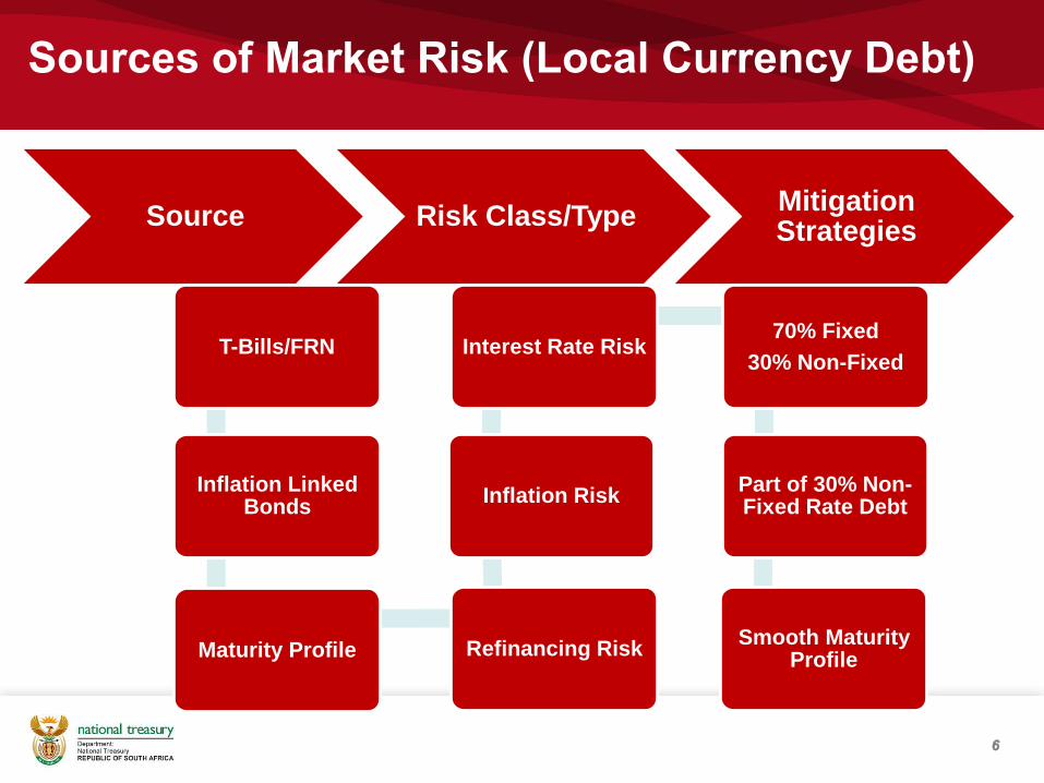
Sources of Market Risk (Local Currency Debt)

Source Risk Class/Type Mitigation Strategies

T-Bills/FRN

Inflation Linked Bonds

Maturity Profile Refinancing Risk

Inflation Risk

Interest Rate Risk 70% Fixed

30% Non-Fixed

Part of 30% Non-Fixed Rate Debt

Smooth Maturity Profile

7

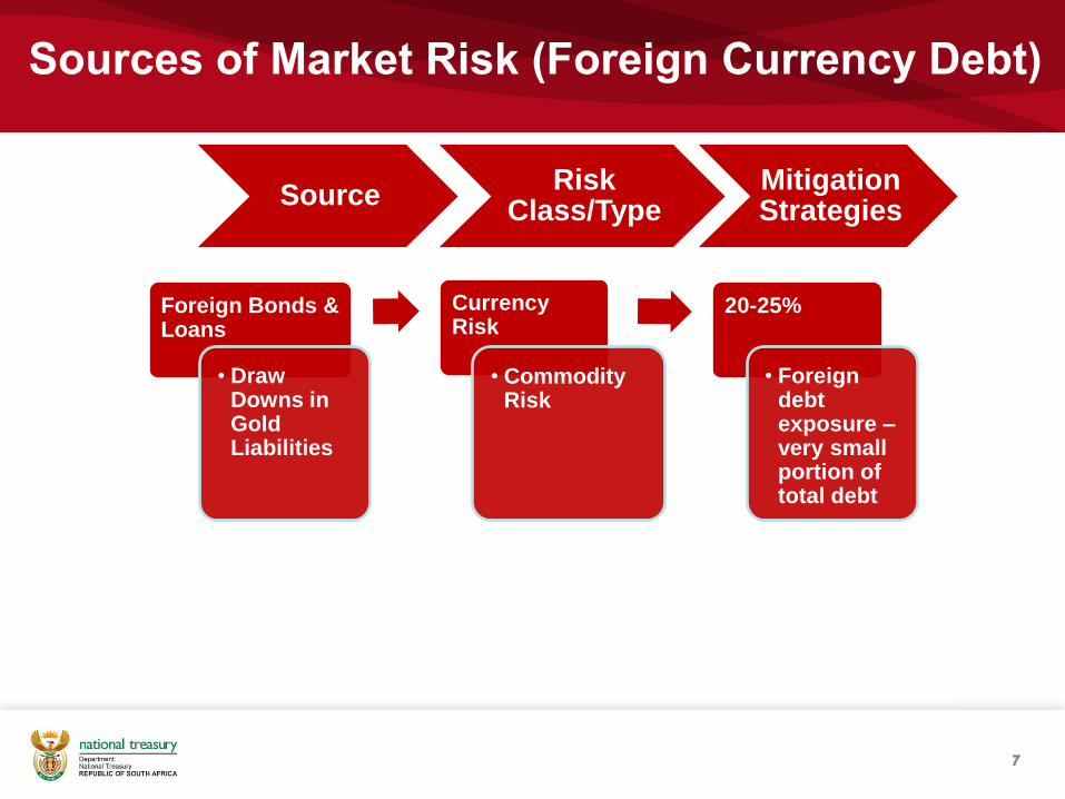
Sources of Market Risk (Foreign Currency Debt)

Source Risk

Class/Type Mitigation Strategies

Foreign Bonds & Loans

• Draw Downs in Gold Liabilities

Currency Risk

• Commodity Risk

20-25%

• Foreign debt exposure – very small portion of total debt

8

Currency Risk Indicators

• Portfolio Risk

– Foreign debt as a % of total debt

• Debt Sustainability Risks

– Total foreign debt as % of GDP

– Foreign currency debt/int. pmt as % of Tax revenue from exports

– Current Account Deficit as % of GDP

– Exchange rate volatility

– Foreign currency liability as % of reserves

9

Currency Risk Techniques and Mitigation

Strategies

• Techniques

– Value at Risk

– Cost at Risk

– Probability Forecast Model

• Mitigation Strategies

– 20% exposure to the risk factor with a permissible upward deviation

of 5%

10

Example 1: Value@Risk – Foreign Currency Debt

Summary Statistics – June 2013

Correlation Matrix – June 2013

Value Position (Outstanding Foreign Currency Debt in USDZAR, EURZAR, ZARJPY)

Value-at-Risk Amounts – June 2013

11

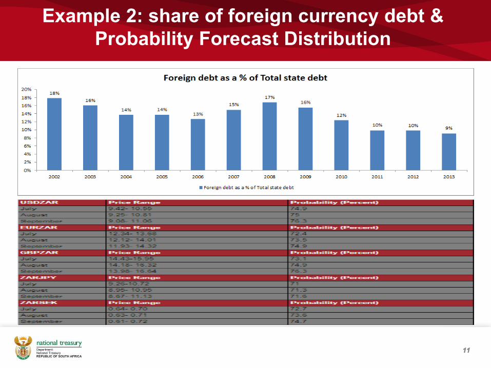
Example 2: share of foreign currency debt &

Probability Forecast Distribution

12

Refinancing Risk Indicators

• Share of debt maturing in 12 months

• Average Term to maturity

– Historical ATM

– Current portfolio ATM

• Smooth maturity profile

13

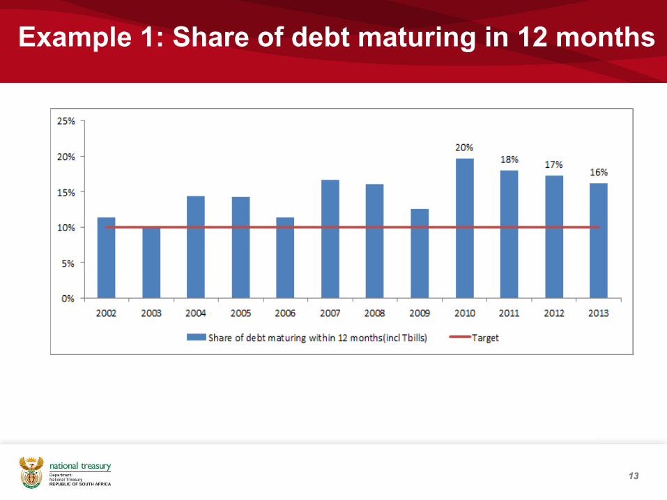
Example 1: Share of debt maturing in 12 months

14

Example 2: historical and current portfolio ATM

15

Example 3: Smooth maturity profile

• Maximum amount Government is comfortable redeeming in a fiscal year.

- Based on cash expectation and time value of money.

• FRB (Nominal) and ILB (Valued to redemption)

• Above the line would have to be switched.

• Maximum Limits in Fixed Rate and inflation linked bonds.

16

Inflation Risk Indicators

• Portfolio Risk

– Share of revalued CPI debt as % of domestic debt

– ATM of Inflation linked debt

– Break-even inflation

• Debt Sustainability

– Share of revalued CPI debt as % of GDP

– Deviation from the upper target band

– Cyclicality of inflation to Revenue

– Volatility of oil price and exchange rate

17

Inflation Risk Techniques and Mitigation

Strategies

• Techniques

– Geometric Brownian Motion (GBM model)

– Cost at Risk on revalued Inflation-linked bonds

• Mitigation Strategies

– Non-fixed rate debt (T-bills and inflation linked debt) limited to 30 per

cent of the domestic debt portfolio.

18

Example 1: Inflation Risk Indicators

19

Example 2: Inflation Risk Techniques

20

Interest Rate Risk Indicators

• Portfolio Risk

– Level, slope and curvature (sources of variation – yield curve risks)

– Interest rate composition (fixed versus non-fixed)

• Debt Sustainability

– Debt service cost as % of revenue and GDP

– Impact of interest rate debt on tax revenue

21

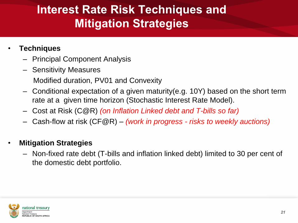
Interest Rate Risk Techniques and

Mitigation Strategies

• Techniques

– Principal Component Analysis

– Sensitivity Measures

Modified duration, PV01 and Convexity

– Conditional expectation of a given maturity(e.g. 10Y) based on the short term

rate at a given time horizon (Stochastic Interest Rate Model).

– Cost at Risk (C@R) (on Inflation Linked debt and T-bills so far)

– Cash-flow at risk (CF@R) – (work in progress - risks to weekly auctions)

• Mitigation Strategies

– Non-fixed rate debt (T-bills and inflation linked debt) limited to 30 per cent of

the domestic debt portfolio.

22

Example 1: Interest Rate Risk Techniques

Analysis of Yield Curve Risk – March 2013 Analysis of Yield Curve Risk – June 2013

• The purpose of PCA is to uncorrelate risk factor movements, therefore reducing

dimensions in a huge data set.

• It is used to identify the key drivers of term structure movements, and will suggest factors/

parameters that explain most of the variability in both yields and changes in yields.

• The weights in the linear combination are determined by eigenvectors and eigenvalues are

variances of the principal components.

• The principal components are ordered according to the size of eigenvalue, so that the first

principal component (the one with largest variance) explain most of the variation.

• It explains the variance-covariance structure of the original variables through an orthogonal

rotation such that the first principal component gives the direction of maximum variation.

• The second gives the next largest direction of maximum variability orthogonal to the first

principal component and the third principal component.

23

Example 2: Stochastic Interest Rate Model

• Vasicek model describes interest rate movements as driven by only one

source of market risk.

• In linking bond yields and prices of long term bonds (mainly zero coupon

bonds) to the short rate model, one key assumptions of the model is that

for any maturity, the bond yield (or spot rate) is a linear function of the

current short term interest rate.

• Complete dependence on the current short term interest rates implies

that in a less realistic and simple financial market, the current level of

short term rates are enough to tell a complete shape of the yield curve,

given some model parameters.

24

Example 2: Continued

25

Market Risk Rating Methodology

26

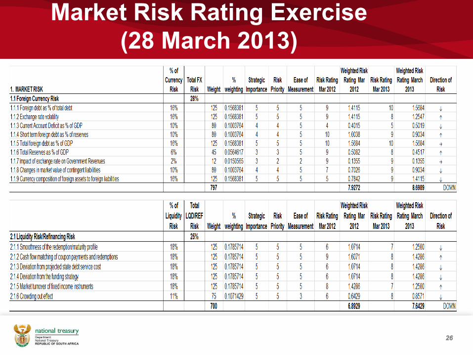
Market Risk Rating Exercise

(28 March 2013)

27

Market Risk Rating Exercise

(28 March 2013)

28

Thank You

29

First Benchmark – 1999/2000

1. Employ a polynomial framework for modeling risk

2. Apply to Heath-Jarrow-Morton model of interest rates and FX

3. Overlay a debt management strategy and calculate its costs and risk

4. Repeat many strategies and deduce cost and risk as a function of strategy and assumptions

5. Determine robust efficient benchmarks

30

• Domestic interest rate exposure (duration) = primary source of risk

• Foreign debt (or currency exposure) provides cost savings and

diversification = determinant of efficiency

First Benchmark Results

Proposal Duration FGN

A 4.00 7.4%

B 3.85 10.0%

C 3.85 15.0%

Current 4.16 7.4%

Current Debt Portfolio

D = 4.2; ZAR = 100%

D = 3.2; ZAR = 100%

D = 4.2; ZAR = 70%

D = 3.2; ZAR = 70%

Current Debt PortfolioCurrent Debt Portfolio

D = 4.2; ZAR = 100%

D = 3.2; ZAR = 100%

D = 4.2; ZAR = 70%

D = 3.2; ZAR = 70%

1: Base Case

31

Second Benchmark 2005/06

“From a Duration Target to Optimal Debt Portfolio”

• Duration measure depends on interest rate changes – not

controllable.

• Duration measure may contradict with the strategy to lengthen

maturity profile of the debt portfolio.

• Duration remains a good measure of cost reduction (in the long

term) but not risk reduction.

• Optimal debt portfolio aims to find the most efficient allocation

(between fixed & non-fixed) that minimises the debt cost subject to

prudent risk level.

32

Valuation of the Debt Portfolio

• Create a single platform for entire debt portfolio

• Develop a valuation calculator

• Analyse the debt portfolio

– Fixed versus non-fixed

– Domestic versus foreign

– Maturity profile

– Debt as % of GDP

• Calculate debt portfolio analytics

• For marketable debt:

– Actual yield curve used to calculate discount factors and NPV

• For non-marketable domestic debt:

– Priced off the government yield curve

• For non-marketable foreign debt

– An average spread of RSA paper issued in the relevant foreign

currency is added to the foreign yield curve

33

Determining the Benchmark

• Simulation of historic portfolios consisting of the following 5

funding instruments:

– Floating (ZAR) debt (treasury bills)

– Fixed 5-year ZAR debt

– Fixed 10-year ZAR debt

– Fixed 5-year US$ debt

– Fixed 10-year US$ debt

• Choice of funding instruments informed by available data points

34

Simulation Process

• Assume a constant monthly issuance (to address re-financing risk)

• Different portfolio combinations are run about 20000 times (weights kept constant)

• Sorted in nominal and marked to market terms

• Portfolio with smallest nominal amount is the optimal

• Penalty function introduced to calculate the cost of deviating from the optimal

35

Benchmark Results

• Best (cheapest) strategy

– 100% of 5 year ZAR fixed rate debt

• 2nd best strategy

– 10% ZAR floating and 90% 5yr ZAR fixed rate debt

• Best strategy (overall portfolio)

– 10% ZAR floating, 80% 5yr ZAR fixed rate debt and 10% 5yr

US$ fixed rate debt

36

Cost-at-Risk Exercise

• 10000 econometric simulations

• Baseline based on a collaborative projection of risk drivers

• Probability distributions of risk drivers determined

• Calculate deviation from expected debt service cost based on

– Future evolution of risk drivers and

– Expected borrowing requirements

37

Benchmarking Flow Diagram

38

Third Benchmark 2012-13

Inputs

• Cash-flows

• Primary deficit

• Financial variables

• Fiscal variables

Process

• Strategies

• Shocks

• Allocations

Outputs

Cost Indicators • Debt Service-cost to GDP

• Debt Service-cost to Revenue

• Debt to GDP

• Expenditure to Revenue

• Revenue to GDP

Sensitivity Indicators • Average Time to Maturity

• Share of debt maturing in 12 months

• Share of Inflation-linked debt to Domestic

debt

• Fixed versus Floating debt

• Fixed versus Inflation-linked debt

39

Conclusion

• Debt instruments for risk benchmarks are limited to few liquid benchmark

issues.

• A pure historical approach to a risk benchmark may be easy to explain,

but the future evolving similar to the past is a serious issue in forward

looking risk analysis.

• History should be used to derive parameters (mean and standard

deviation) and then use that to simulate the future evolution to arrive at a

range of outcomes.

• A deterministic approach such as the MTDS is a perfect start in

preparation to move to a stochastic framework.

• As part of internal capacity building - It is never a waste of time

understanding the pricing/cash flow and risk characteristics of debt

instruments, e.g. inflation linked bonds in RSA case.

• A move from excel to system environment also needs a balance of

human resource skills in Statistics/Mathematics, Finance,

Economics/metrics. IT/Computer Science skills will be a plus!

40

Thank You