workshop preprints quasoq 2016 - swc preprints quasoq 2016. 4. th. international workshop on...

Workshop Preprints

QuASoQ 20164th International Workshop on Quantitative Approaches to Software Quality

co-located with APSEC 2016Hamilton, New Zealand, December 6th , 2016

Editors:

Horst Lichter, RWTH Aachen University, GermanyToni Anwar, UTM Johor Bahru, MalaysiaThanwadee Sunetnanta, Mahidol University, ThailandKonrad Fögen, RWTH Aachen University, Germany

Table of Contents

Trying to Increase the Mature Use of Agile Practices by Group Development Psychology Training - An Experiment

3

Lucas Gren and Alfredo Goldman

Predicting Quality of Service (QoS) Parameters using Extreme Learning Machines with Various Kernel Methods

11

Lov Kumar, Santanu Rath and Ashish Sureka

Local Variables with Compound Names and Comments as Signs of Fault-Prone Java Methods

19

Hirohisa Aman, Sousuke Amasaki, Tomoyuki Yokogawa and Minoru Kawahara

Towards improved Adoption: Effectiveness of Research Tools in Real World 27 Richa Awasthy, Shayne Flint and Ramesh Sankaranarayana

Code Coverage Analysis of Combinatorial Testing 34 Eun-Hye Choi, Osamu Mizuno and Yifan Hu

Sustainability Profiling of Long-living Software Systems 41 Ahmed Alharthi, Maria Spichkova and Margaret Hamilton

Improving Recall in Code Search by Indexing Similar Codes under Proper Terms 49 Abdus Satter and Kazi Sakib

Organization

Horst Lichter (Chair), RWTH Aachen University, Germany Toni Anwar (Co-Chair), UTM Johor Bahru, Malaysia Thanwadee Sunetnanta (Co-Chair), Mahidol University, Thailand Matthias Vianden, Aspera GmbH, Aachen, Germany Wan M.N. Wan Kadir, UTM Johor Bahru, Malaysia Taratip Suwannasart, Chulalongkorn Univiversity, Thailand Tachanun Kangwantrakool, ISEM, Thailand Jinhua Li, Qingdao University, China Apinporn Methawachananont, NECTEC, Thailand Jarernsri L. Mitrpanont, Mahidol University, Thailand Nasir Mehmood Minhas, PMAS - AAUR Rawalpindi Pakistan Chayakorn Piyabunditkul, NSTDA, Thailand Maria Spichkova, RMIT University, Melbourne, Australia Sansiri Tanachutiwat, Thai German Graduate School of Engineering, TGGS, Thailand Hironori Washizaki, Waseda University, Japan Hongyu Zhang, Tsinghua University, China

QuASoQ 2016 Workshop Preprints

1

Trying to Increase the Mature Use of Agile Practicesby Group Development Psychology Training

— An Experiment

Lucas GrenChalmers and the University of Gothenburg

Gothenburg, Sweden 412–92 andUniversity of Sao Paulo

Sao Paulo, Brazil 05508–090Email: [email protected]

Alfredo GoldmanUniversity of Sao Paulo

Sao Paulo, Brazil 05508–090Email: [email protected]

Abstract—There has been some evidence that agility is con-nected to the group maturity of software development teams. Thisstudy aims at conducting group development psychology trainingwith student teams, participating in a project course at university,and compare their group effectiveness score to their agility usageover time in a longitudinal design. Seven XP student teams weremeasured twice (43+40), which means 83 data points divided intotwo groups (an experimental group and one control group). Theresults showed that the agility measurement was not possibleto increase by giving a 1.5-hour of group psychology lectureand discussion over a two-month period. The non-significantresult was probably due to the fact that 1.5 hours of trainingwere not enough to change the work methods of these studentteams, or, a causal relationship does not exist between the twoconcepts. A third option could be that the experiential settingof real teams, even at a university, has many more variablesnot taken into account in this experiment that affect the twoconcepts. We therefore have no conclusions to draw based on theexpected effects. However, we believe these concepts have to beconnected since agile software development is based on teamworkto a large extent, but there are probable many more confoundingor mediating factors.

I. INTRODUCTION

Agile Project Management and its methods evolved duringthe nineties on ideas from lean production and more flexibleproduct development [1], but also from practical experiencesaving IT projects that were about to fail [2]. The main differ-ence between lean production and agile project managementis that both management ideas admit they do not know whatthe best end-product would look like far in advance [3]. Theagile development processes are often intimately connectedto high performing, self-managing and mature teams [4] andthe way group norms are set has been shown to increaseperformance [5]. Agile development, as compared to plan-driven ditto, implies more communication and focus on humanfactors, which make the group psychology aspects of teamsa key ingredient [6]. However, the agile processes do notexplicitly include the temporal perspective of what happensto all teams over time from a group maturity perspective.

In this experiment, we conducted a longitudinal study ofseven agile teams to see if the group development affectsprocess agility. By giving half of the teams training in group

psychology theory we hoped to see an effect on their measuredagility. However, by only giving a 1.5-hour lecture, we did notsee such an effect. We instead discuss reasons for our non-significant results and suggest next steps for future attempts atfinding such effects in complex social systems.

We follow Jedlitschka, Ciolkowski and Pfahl’s [7] guide-lines on how to to report experiments on software engineeringthroughout this paper. We will therefore start by giving atheoretical background (Section II), describe the experimentin detail (Section III), analyze the data and show descriptivestatistics and tests (Section IV), and, finally, discuss the result(Section V) and provide conclusions and suggestions for futurework (Section VI).

A. Context

When software development teams transition to an agileapproach (i.e. more team-based work) more of the processis dependent on how well the team cooperates [4]. The agileadoption sometimes fails due to the fact that an agile transitionis a cultural change as well, which impose new constellationsof teams [8], [9]. To further explore the causal relationshipbetween the group dynamics and agile practices over time,would therefore be interesting, both from a research and anindustrial perspective, in order to guide agile adoptions better.

B. Problem statement

Many aspects of group dynamics come into play in theteam-based workplace [10]. There are studies showing acorrelation between group maturity and agile concepts (seee.g. [11]), however, little is known of any causal relationshipbetween them. Correlation analysis only show the connectionbetween the two. If the mature usage of agile practices aredirectly dependent on group development aspects has not yetbeen investigated. Therefore, it would be interesting to seeif group psychology training of agile software developmentteams could increase the adoption of concrete agile practices.


3

II. BACKGROUND

A. Agile methods (processes)

Agile methodologies can be seen as an approach ratherthan a technique that mostly change the culture and valuesbehind managing projects. There are some more concrete agilemethods, but they all basically share the same values. However,in order to understand how these methods work in practice, wewill now shortly present some of the agile practices and howthe values are implemented.

a) eXtreme programming (XP): eXtreme programmingwas the first method created by the agile community and isthe most researched method [12] and is considered relativelystrict and controlled. The practices that implement the agileprinciples are [13]:

1) The planning game. In the beginning of each iter-ation, the team, managers, and customers meet andwrite requirements in form of user stories (written inclear natural language and in a way that everybodycan understand). During these meetings the wholegroup estimates and prioritizes the requirements.

2) Small releases. Working software is up and runningand delivered very fast and new versions are releasedcontinuously, from every few days to every fewweeks.

3) Metaphor. Customers, managers, and developersmodel the system after a constructed metaphor or setof metaphors.

4) Simple design. Developers are asked to keep designas simple as possible.

5) Tests. The development is test-driven (TDD), i.e., thetest are written before the code.

6) Re-factoring. The code should be revised and simpli-fied over time.

7) Pair-programming. All code is written by having twodevelopers per machine.

8) Continuous integration. The developers integrate newcode into the system as often as possible. However, allcode must pass the testing otherwise it is discarded.

9) Collective ownership. Developers can change codewherever necessary and the overall code is assessed.

10) On-site customer. A customer is in the team all thetime to answer questions so the team always worksaccording to what is needed.

11) 40-hour work week. The team works with a sus-tainable pace defined as a 40 hour work week. Therequirement selected for each iteration should nevermean that the team needs to work overtime.

12) Open workspace. The team should be collocated andfit in the same room. The layout of the room shouldmake cooperation and communication easy.

b) Scrum: Scrum is based on XP and is one of themore common methodologies and is built on embracing changeand focus a lot on delivering value. In Scrum, the projecthas a prioritized backlog of requirements and use iterativedevelopment (called “sprints”) to get basic working softwarefor the customer to view as soon as possible. Scrum uses self-organizing teams that get coordinated through daily meetingscalled “scrums.” The manager is called a “Scrum Master” toclarify that it is a facilitating role and not a directive one.

The Scrum methodology consists of three main phases:Pre-sprint planning, sprint (iteration), and post-sprint meeting.All work to be done is kept in a “release backlog” wherefrom requirements (user stories) are taken to the current “sprintbacklog.” The requirements are usually broken down from ahigher abstraction level when the sprint backlog is made. Theactual sprint (usually 2–4 weeks) is when the implementationis performed. Here, the sprint backlog is frozen and the team“sprints” to complete what was planned. The team memberschoose tasks they want to work on themselves. “Scrum meet-ings” also called “Daily scrums” are 15-minute meetings everymorning were the team members check status, report problems,and keep the whole team focused on a common goal. Thepost-meeting is done to evaluate the process and demonstratethe current system. One important aspect of Scrum is to havesmall working teams in order to maximize communication,minimize overhead, and maximize the sharing of informal (ortacit) knowledge. The team should also agree and be able todefine when something is considered “done” [14].

c) Lean and Kanban: The flexible project managementtechniques and focus on customer value is not new. Withinlean manufacturing these aspects have existed a long time (formore information about lean manufacturing see for example[15]). Many companies combine the process of Scrum withKanban (Scrum-ban). It is important to note that Kanban is asignal card to pull products through the process within Leanproduction but has become a software development tool itself[16]. Scrum is a more strict process and can be modifiedby changing the WIP (work in progress) in each sprint intobeing connected to the work-flow state to prevent too muchWIP. Kanban also allows adding items within each sprint.Another aspect is to change the sprint backlog owned by theteam into a Kanban board with multiple teams with work-flowstate instead. The Kanban board is never reset after a sprintand can be followed over time, and is also less dependenton collocation. Scrum only allows three different roles of theteam, while Kanban does not have a limit. Therefore, largerteams in larger organization with a diversity of specializationsoften use Kanban or Scrum-ban when possible [17].

d) Crystal: We will not describe the Crystal method-ologies in detail but, generally speaking, they are built on theassumption that the main problem in software development ispoor communication. Crystal focuses on people, interaction,community, skills, talents, and communication as main effectson performance [18].

The twelve agile principles are a very high-level descriptionof a work environment. Agile software development is anambiguous concept with descriptions on various levels ofabstraction. Many of these are obviously connected to groupdynamics. The problem is that these psychological aspects arenot described in detail in the methods (processes). This meansthat this dimension is left out for practitioners to figure our forthemselves to a large extent. In order to try to operationalizeagility and correlate the measurement to group maturity overtime, we enforced the twelve original XP practices (describedin Section II-A0a) on all the participating student teams andthen opted to use the Perceptive Agile Measurement developedby So and Scholl [19] in order to measure this “agile” behaviorover time. All the items are included in Section III-E.


4

B. Groups and Teams

A group can be defined as: “three or more members thatinteract with each other to perform a number of tasks andachieve a set of common goals” [20]. If the group is largerall the members might not have a common goal, which meansthat larger groups often consist of subgroups. Some studieshave shown that smaller groups are more productive thanlarger groups with a threshold at around eight individuals [21].In psychology, a “work-group” is a group that has a sharedview of the group goal and has developed a structure thatenables goal achievement. A team, on the other hand, isan effective work-group, however, we will use the termssomewhat interchangeably in this paper, since agile work-groups are called “teams” no matter their actual effectiveness.In social psychology, though, only 17% of all groups wereconsidered teams according to one study [22].

The group research in psychology received much attentionafter the second world war and before the sixties. Afterthat, the focus in research was on the individual insteadof groups [22]. The start of the human factors research insoftware engineering has also mostly focused on individualsand their personalities and traits for 40 years without findingany coherent results [23]. Therefore, we have reason to believethat much of what happens in software engineering is set onteam-level, which means that “agility” is hard to obtain if wedo not understand the group dynamics of agile teams, or asWheelan and Hochberger [22] very adequately put it: “beforeone jumps to fix something, one has to know what is broken.”

During so many years of research on groups in psychology,there are, of course, a diversity of group development models[24]. However, there seems to be a reoccurring patterns of whathappens to all types of groups when humans get together inorder to solve a task. The first researchers to aggregate modelsinto a general group development model were Tuckman andJensen [25] in the seventies. In the nineties Susan Wheelandid a similar aggregation of existing models that resulted inthe Integrated Model of Group Development that we usedin this study. However, Tuckman and Jensen’s [25] modelwith the phases; Forming, Storming, Norming, and Performingcorrespond well to the stages suggest by Wheelan [22].

C. Wheelan’s Integrated Model of Group Development

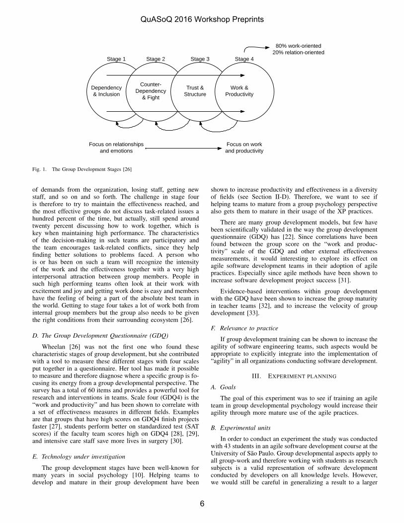
The Integrated Model of Group Development (or IMGD)describes four different stages that all groups go throughin their journey towards becoming a well-functioning highperforming team. These stages are illustrated in Figure 1 anddescribed next. The Group Development Questionnaire (theGDQ), that is a measurement of how much energy the groupis spending on each development stage, is described afterward.

a) Stage 1 — Dependency and Inclusion: During thefirst stage of group development (i.e. when the group is new)the group members have more focus on safety and inclusion,a dependency on the designated leader, and more of a wishfor order and structure, than in more mature stages. A groupat stage one can still get work done, but will focus moreon figuring out who the other people are. There is a lackof structure and the group needs to become organized, beingable to do efficient work, and achieve the group goals. Thegroup members need to create a sense of belonging and lay

the foundation for how to interact within the group. At this firststage, there is a lack of the feeling of belonging to a group,but after this stage people start feeling safe enough to statetheir ideas and contribute to how they think the group shouldwork in order to achieve its goals. If this does not happengroups stagnate, which is often noticed when group membersstop doing work between meetings and even stop attending thegroup meetings [22].

b) Stage 2 — Counter-Dependency and Fight: Duringthe second stage the group starts having conflict. These differ-ences in opinion is a must in order to create clear roles basedon real competence and to make it possible to work together ina constructive manner. The group members have to go throughthis more turbulent stage in order to build trust. After feelingsafe and therefore daring to have these conflicts, a sense ofloyalty emerges, which is needed to create cohesion. Since wedo not have a clear picture of goals and roles in the beginning,we need this emotional and hard work in order to get sharedperceptions of values, norms, and goals, which need to be seton group-level. Since everybody needs to believe in the groupvalues and norms for them to fill their purpose, the rules ofthe game need to be negotiated so that all members thoroughlybelieve in them. The more shallow discussions about goalsprobably present in the first stage, will now be more emotionalor include disagreements [22].

c) Stage 3 — Trust and Structure: During the thirdstage the structure is getting into place and the roles are nowactually based on competence instead of status, power, orsafety concerns. The communication patterns are more openand also more task-oriented. In this stage the role, organization,and process negotiations are most often more mature and therewill be an evident clarification and consensus regarding thegroup goals. The group members also spend time solidifyingpositive relationships, and when the tasks are adjusted tocompetence the likelihood of goal achievement is higher. Atthis stage the leader’s roll goes from needing to have been moredirective to being more consultative. The communication struc-ture is also more flexible (i.e. group members talk to whomeverthey need). Along the group development the content of thecommunication is also more and more task-oriented insteadof relation-oriented. Groups always need the relation-orientedcommunication since we always need to do the maintenanceof discussing how we work together as a group. Therefore,conflict will still occur but be over much faster since the grouphas better conflict management techniques. Work satisfactionand cooperation increase together with cohesion and trust. Atthis stage the individual commitment to the group goal willbe higher (i.e. we care about what the group is doing on apersonal level). This means we will see a voluntary conformitywith the norms and helpful deviation from the group (like sub-grouping) will be accepted if considered helpful for the groupas a whole [26].

d) Stage 4 — Work and Productivity: The forth stageof group development is when the group does even betterwith regards to the purpose of stage three. This means thatthe group focuses on getting the task done well together aswell as maintaining group cohesion over a longer period oftime. It is important to realize that there is a large set ofvariables that can and will disturb the group development.Basically, all changes will have such an effect, e.g. change


5

Stage 1 Stage 2 Stage 3 Stage 4

Dependency& Inclusion

Counter-Dependency

& Fight

Trust &Structure

Work &Productivity

Focus on relationshipsand emotions

Focus on workand productivity

80% work-oriented20% relation-oriented

Fig. 1. The Group Development Stages [26]

of demands from the organization, losing staff, getting newstaff, and so on and so forth. The challenge in stage fouris therefore to try to maintain the effectiveness reached, andthe most effective groups do not discuss task-related issues ahundred percent of the time, but actually, still spend aroundtwenty percent discussing how to work together, which iskey when maintaining high performance. The characteristicsof the decision-making in such teams are participatory andthe team encourages task-related conflicts, since they helpfinding better solutions to problems faced. A person whois or has been on such a team will recognize the intensityof the work and the effectiveness together with a very highinterpersonal attraction between group members. People insuch high performing teams often look at their work withexcitement and joy and getting work done is easy and membershave the feeling of being a part of the absolute best team inthe world. Getting to stage four takes a lot of work both frominternal group members but the group also needs to be giventhe right conditions from their surrounding ecosystem [26].

D. The Group Development Questionnaire (GDQ)

Wheelan [26] was not the first one who found thesecharacteristic stages of group development, but she contributedwith a tool to measure these different stages with four scalesput together in a questionnaire. Her tool has made it possibleto measure and therefore diagnose where a specific group is fo-cusing its energy from a group developmental perspective. Thesurvey has a total of 60 items and provides a powerful tool forresearch and interventions in teams. Scale four (GDQ4) is the“work and productivity” and has been shown to correlate witha set of effectiveness measures in different fields. Examplesare that groups that have high scores on GDQ4 finish projectsfaster [27], students perform better on standardized test (SATscores) if the faculty team scores high on GDQ4 [28], [29],and intensive care staff save more lives in surgery [30].

E. Technology under investigation

The group development stages have been well-known formany years in social psychology [10]. Helping teams todevelop and mature in their group development have been

shown to increase productivity and effectiveness in a diversityof fields (see Section II-D). Therefore, we want to see ifhelping teams to mature from a group psychology perspectivealso gets them to mature in their usage of the XP practices.

There are many group development models, but few havebeen scientifically validated in the way the group developmentquestionnaire (GDQ) has [22]. Since correlations have beenfound between the group score on the “work and produc-tivity” scale of the GDQ and other external effectivenessmeasurements, it would interesting to explore its effect onagile software development teams in their adoption of agilepractices. Especially since agile methods have been shown toincrease software development project success [31].

Evidence-based interventions within group developmentwith the GDQ have been shown to increase the group maturityin teacher teams [32], and to increase the velocity of groupdevelopment [33].

F. Relevance to practice

If group development training can be shown to increase theagility of software engineering teams, such aspects would beappropriate to explicitly integrate into the implementation of“agility” in all organizations conducting software development.

III. EXPERIMENT PLANNING

A. Goals

The goal of this experiment was to see if training an agileteam in group developmental psychology would increase theiragility through more mature use of the agile practices.

B. Experimental units

In order to conduct an experiment the study was conductedwith 43 students in an agile software development course at theUniversity of Sao Paulo. Group developmental aspects apply toall group-work and therefore working with students as researchsubjects is a valid representation of software developmentconducted by developers on all knowledge levels. However,we would still be careful in generalizing a result to a larger


6

population than that of developers in the phase of learning anagile approach (i.e. individuals with little experience of agilesoftware development in practice). The course were offeredto 3rd year students, however, most students usually take thecourse in the 4th or 5th (last) year of their software engineeringdegree. The course is also open to graduate students whoare given the possibility to take the course twice during theirgraduate education.

The student teams in this study comprised students en-rolled in a project XP software development course called“The Laboratory of XP” at the Institute of Mathematics andStatistics at the University of Sao Paulo. The purpose of thecourse is to introduce agile methods through the use of XP.These methods included, at a minimum, the twelve practicespresented in Section II-A0a. Some other staff at the universityacted as customers and had to pitch their project ideas to thestudents, who signed up for the most interesting one from theirpoint of view. All the teams included six to eight membersand a more experienced student acting as a an agile coach forthe team. The process was put together by the student teamsthemselves and we allowed any type of additional practicesthey selected as long as it was within the XP framework. Asan example, we enforced collocation of a minimum of eighthours per week.

C. Experimental material

The experimental object was the agile software develop-ment team. Group norms and cooperation are set on grouplevel and therefore the actual “team” is the relevant level ofanalysis.

D. Tasks

The experimental tasks applied in this experiment was forthe teams (one team at a time) to listen and reflect on groupdevelopment theory and discuss its applicability in connectionto their own team.

E. Hypotheses, parameters, and variables

The construct used to measure agile practices and thebehavior connected to them, was the mature usage of nineagile practices as defined by So and Scholl [19]:

Iterative Planning: (1) All members of the technical team actively partici-pated during iteration planning meetings. (2) All technical team members took partin defining the effort estimates for requirements of the current iteration. (3) Wheneffort estimates differed, the technical team members discussed their underlyingassumption. (4) All concerns from team members about reaching the iterationgoals were considered. (5) The effort estimates for the iteration scope items weremodified only by the technical team members. (6) Each developer signed up fortasks on a completely voluntary basis. (7) The customer picked the priority of therequirements in the iteration plan.

Iterative Development: (1) We implemented our code in short iterations. (2)The team rather reduced the scope than delayed the deadline. (3) When the scopecould not be implemented due to constraints, the team held active discussions onre-prioritization with the customer on what to finish within the iteration. (4) Wekept the iteration deadlines. (5) At the end of an iteration, we delivered a potentiallyshippable product. (6) The software delivered at iteration end always met qualityrequirements of production code. (7) Working software was the primary measurefor project progress.

Continuous Integration and Testing: (1) The team integrated continuously.(2) Developers had the most recent version of code available. (3) Code was checkedin quickly to avoid code synchronization/integration hassles... (4) The implementedcode was written to pass the test case. (5) New code was written with unit testscovering its main functionality. (6) Automated unit tests sufficiently covered allcritical parts of the production code. (7) For detecting bugs, test reports fromautomated unit tests were systematically used to capture the bugs. (8) All unittests were run and passed when a task was finished and before checking in andintegrating. (9) There were enough unit tests and automated system tests to allowdevelopers to safely change any code.

Stand-Up Meetings: (1) Stand up meetings were extremely short (max. 15minutes). (2) Stand up meetings were to the point, focusing only on what hadbeen done and needed to be done on that day. (3) All relevant technical issuesor organizational impediments came up in the stand up meetings. (4) Stand upmeetings provided the quickest way to notify other team members about problems.(5) When people reported problems in the stand up meetings, team membersoffered to help instantly.

Customer Access: (1) The customer was reachable. (2) The developers couldcontact the customer directly or through a customer contact person without anybureaucratic hurdles. (3) The developers had responses from the customer in atimely manner. (4) The feedback from the customer was clear and clarified hisrequirements or open issues to the developers.

Customer Acceptance Tests: (1) How often did you apply customer accep-tance tests? (2) A requirement was not regarded as finished until its acceptancetests (with the customer) had passed. (3) Customer acceptance tests were used asthe ultimate way to verify system functionality and customer requirements. (4) Thecustomer provided a comprehensive set of test criteria for customer acceptance. (5)The customer focused primarily on customer acceptance tests to determine whathad been accomplished at the end of an iteration.

Retrospectives: (1) How often did you apply retrospectives? (2) All teammembers actively participated in gathering lessons learned in the retrospectives.(3) The retrospectives helped us become aware of what we did well in thepast iteration/s. (4) The retrospectives helped us become aware of what weshould improve in the upcoming iteration/s. (5) In the retrospectives (or shortlyafterwards), we systematically assigned all important points for improvement toresponsible individuals. (6) Our team followed up intensively on the progress ofeach improvement point elaborated in a retrospective.

Collocation: (1) Developers were located majorly in... (2) All members ofthe technical team (including QA engineers, db admins) were located in... (3)Requirements engineers were located with developers in... (4) The project/releasemanager worked with the developers in... (5) The customer was located with thedevelopers in...

The group maturity (or effectiveness) operationalizationwas done through using Scale 4 of the GDQ [22]. All theitems in the GDQ scale cannot be shared here due to copyright,however, we can include three example items:

• The group gets, gives, and uses feedback about itseffectiveness and productivity.

• The group acts on its decisions.

• This group encourages high performance and qualitywork.

The group development measurement on Scale 4 wasassessed on a 5-point Likert scale (1 = low agreement tothe statement and 5 = high agreement). The agile itemswere assesses on a 7-point Likert scale (1 = never and 7 =


7

always). These scales were used for the simple reason thatthese measurements were developed and validated using theseexact scales.

Both measurements have been validated using a factoranalysis [34] and a test for internal consistency (using theCronbach’s α [35]).

The formal research hypothesis for each scale is thatthe mean values for the scale is different between the twomeasurements, or H1 : µ1 6= µ2.

F. Design

We used a longitudinal research design in order to test dif-ferences in group mean value scores on the two measurementsover time. The first measurement comprised seven teams and43 student responses, and the second measurement comprisedthe same seven teams with 40 responses, i.e. three student wereabsent during the second measurement.

G. Procedure

The two measurement surveys were distributed to theteams five weeks into their software development projects(during their scheduled and collocated development sessions).The reason was to let the students actually form teams andhave done some work before the first measurement. Threeof the participating seven teams were randomized into theexperimental group and the remaining four teams were used asa control group. The randomization was done by first writingthe numbers “3” and “4” on paper slips and letting a personnot connected to the experiment draw one folded slip for theresearch group (three groups were selected). The second stepwas conducted by writing all team names on other paper slipsand letting the person draw three slips to be used for theresearch group.

On week six, the three selected teams participated in a1.5-hour group development training with a discussion onthe applicability to their own team. During the first hourof the training, the first author of this paper presented TheIntegrated Model of Group Development [10] and its fourgroup developmental stages. The idea is, briefly, that there arepredictable group developmental stages that all groups haveto go through in order to work effectively. If team-membersare aware of these there is a smaller probability of the teamgetting stuck on group issues, which leads to quicker andhigher quality work [10]. Aspects covered were, for example,goal-setting, role clarification, decision-making, and leadershipissues of groups in different development stages.

On week eleven, the second measurement was conductedusing the same procedure as in the first measurement.

H. Analysis procedure

The data was analyzed using a general linear model forrepeated measures (i.e. a standard repeated measures ANOVA).Such a model assumes normality in data, but since we did notfind any significant result, we did not proceed to use non-parametric tests (since these are more restrictive and wouldtherefore neither show any significance).

IV. RESULTS

A. Descriptive statistics

Since we aimed at affecting the agile practices score byconducting group psychology training, we first looked at if wemanaged to increase the group dynamics score. Since that wasnot the case we already knew we did not succeed with theintended plan of the experiment. However, we still looked fordifferences in the agile practices measurement to see if theydiffered anyways between the two measurements. The onlytwo significant differences we found between the first andsecond measurements were that the scales “Retrospectives”and “Customer Acceptance Tests.” Therefore, we show thedescriptive statistics for these scales as well (see Table I).

B. Data set preparation

A mean value was calculated based on the collected datafor each individual, and then for the team according the agilepractices as defined by So and Scholl [19]. The measuredagile practices were: Iteration planning, Iterative development,Continuous integration and testing, Stand-up meetings, Cus-tomer access, Customer acceptance tests, Retrospectives andCollocation. The group development Scale 4 individual itemswere also turned into a mean value for each individual and thenfor the groups separately. Since we wanted to run the analysison group-level we only have three mean values in the researchgroup and four values in the control group (seven groups intotal).

C. Hypothesis testing

Since we have so few data points, we cannot assess thepopulation distribution based on our sample. However, otherstudies have shown this kind of data to be normally distributed[19], [22]. Also, since we did not find any significant resultsbased on parametric tests, neither would we for non-parametrictests (since they are more restrictive). We began by testing thegroup effectiveness score (GDQ4 mean values) for the firstand second measurements and can conclude that we did notsee a significant effect (see Table II).

We then, still, ran the same analysis for all the agilepractices and only found that the scales “Retrospectives” and“Customer acceptance tests” were different between the twomeasurements overall and not in connection to whether theywere in the research group or not (see Table III and Table IV).

We conclude that the group development effectivenessmeasurement (GDQ Scale 4) was not different between theresearch group and the control group (not in the first northe second measurement). The two agile practices “Retrospec-tives” and “Customer acceptance tests” where both differentoverall between the two measurements, but not depending onif the teams were in the research group or the control group.

V. DISCUSSION

We did not find any of the expected results in this study.Clearly, just having 1.5 hours of training and discussion isnot enough to help the group to develop, even if 1.5 hours ofa workweek of 8 hours (like the students in the course had)would be equivalent to 7.5 hours of working full-time 40 hoursa week. When taking a closer look at when other experiments


8

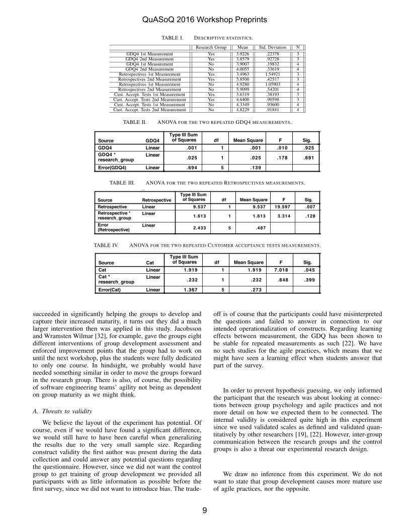
TABLE I. DESCRIPTIVE STATISTICS.

Research Group Mean Std. Deviation NGDQ4 1st Measurement Yes 3.9226 .22378 3GDQ4 2nd Measurement Yes 3.8579 .92728 3GDQ4 1st Measurement No 3.9007 .19832 4GDQ4 2nd Measurement No 4.0055 .33619 4

Retrospectives 1st Measurement Yes 3.4963 1.54921 3Retrospectives 2nd Measurement Yes 5.8500 .42517 3Retrospectives 1st Measurement No 4.9280 1.05903 4Retrospectives 2nd Measurement No 5.9099 .54201 4

Cust. Accept. Tests 1st Measurement Yes 3.6319 .38193 3Cust. Accept. Tests 2nd Measurement Yes 4.6400 .90598 3Cust. Accept. Tests 1st Measurement No 4.3349 .93600 4Cust. Accept. Tests 2nd Measurement No 4.8229 .91841 4

TABLE II. ANOVA FOR THE TWO REPEATED GDQ4 MEASUREMENTS.Tests of Within-Subjects Contrasts

Measure: MEASURE_1Measure: MEASURE_1Measure: MEASURE_1

Source GDQ4Type III Sum

of Squares df Mean Square F Sig.GDQ4 LinearGDQ4 * research_group

Linear

Error(GDQ4) Linear

.001 1 .001 .010 .925 .002

.025 1 .025 .178 .691 .034

.694 5 .139

Measure: MEASURE_1Measure: MEASURE_1

Tests of Within-Subjects Contrasts


Source GDQ4Partial Eta

SquaredGDQ4 LinearGDQ4 * research_group

Linear

Error(GDQ4) Linear

.002

.034


Page 1

TABLE III. ANOVA FOR THE TWO REPEATED RETROSPECTIVES MEASUREMENTS.Tests of Within-Subjects Contrasts


Source RetrospectiveType III Sum

of Squares df Mean Square F Sig.Retrospective LinearRetrospective * research_group

Linear

Error(Retrospective)

Linear

9.537 1 9.537 19.597 .007 .797

1.613 1 1.613 3.314 .128 .399

2.433 5 .487




Source RetrospectivePartial Eta

SquaredRetrospective LinearRetrospective * research_group

Linear

Error(Retrospective)

Linear

.797

.399


Page 1

TABLE IV. ANOVA FOR THE TWO REPEATED CUSTOMER ACCEPTANCE TESTS MEASUREMENTS.Tests of Within-Subjects Contrasts


Source CatType III Sum

of Squares df Mean Square F Sig.Cat LinearCat * research_group

Linear

Error(Cat) Linear

1.919 1 1.919 7.018 .045 .584

.232 1 .232 .848 .399 .145

1.367 5 .273




Source CatPartial Eta

SquaredCat LinearCat * research_group

Linear

Error(Cat) Linear

.584

.145


Page 1

succeeded in significantly helping the groups to develop andcapture their increased maturity, it turns out they did a muchlarger intervention then was applied in this study. Jacobssonand Wramsten Wilmar [32], for example, gave the groups eightdifferent interventions of group development assessment andenforced improvement points that the group had to work onuntil the next workshop, plus the students were fully dedicatedto only one course. In hindsight, we probably would haveneeded something similar in order to move the groups forwardin the research group. There is also, of course, the possibilityof software engineering teams’ agility not being as dependenton group maturity as we might think.

A. Threats to validity

We believe the layout of the experiment has potential. Ofcourse, even if we would have found a significant difference,we would still have to have been careful when generalizingthe results due to the very small sample size. Regardingconstruct validity the first author was present during the datacollection and could answer any potential questions regardingthe questionnaire. However, since we did not want the controlgroup to get training of group development we provided allparticipants with as little information as possible before thefirst survey, since we did not want to introduce bias. The trade-

off is of course that the participants could have misinterpretedthe questions and failed to answer in connection to ourintended operationalization of constructs. Regarding learningeffects between measurement, the GDQ has been shown tobe stable for repeated measurements as such [22]. We haveno such studies for the agile practices, which means that wemight have seen a learning effect when students answer thatpart of the survey.

In order to prevent hypothesis guessing, we only informedthe participant that the research was about looking at connec-tions between group psychology and agile practices and notmore detail on how we expected them to be connected. Theinternal validity is considered quite high in this experimentsince we used validated scales as defined and validated quan-titatively by other researchers [19], [22]. However, inter-groupcommunication between the research groups and the controlgroups is also a threat our experimental research design.

We draw no inference from this experiment. We do notwant to state that group development causes more mature useof agile practices, nor the opposite.


9

B. Lessons learned

The largest lesson learned from this experiment is evidentlyto check the level of intervention effort needed to movegroups forward in their development before conducting thiskind of an experiment. We still do not known the effortneeded, but the span is more then one 1.5 hours workshopwith a second measurement two months later, and less thansix to eight workshops of 2–3 hours during a full year withconnected action plans and follow-up. By having more timewith the teams we could have focused even more concretely on,for example, goal-setting, role clarification, decision-making,functional sub-grouping, or leadership issues, like in [32].

VI. CONCLUSIONS AND FUTURE WORK

We obtained an insignificant result of this experiment.We therefore have no conclusions to draw based on theexpected effects. However, we believe these concepts couldstill be connected since agile software development is basedon teamwork to a large extent. We evidently need a largerintervention effort and, of course there could also be moreconfounding or mediating factors we have not thought of inthe context of agile software development teams.

We would like to redo this experiment with more resourcesand be able to give the teams in the research group eight timesmore workshops with connected action plans in order to seeif we can get a similar effect as has been shown with teacherteams [32]. It would, of course, be advantageous to includeas many teams as possible and at multiple universities andcompanies to increase the statistical power of the experiment.

REFERENCES

[1] H. Takeuchi and I. Nonaka, “The new new product development game,”Harvard business review, vol. 64, no. 1, pp. 137–146, 1986.

[2] J. Sutherland, Scrum: The art of doing twice the work in half the time.Random House Business, 2014.

[3] K. Schwaber and M. Beedle, Agile software development with scrum.Upper Saddle River, NJ: Prentice Hall, 2002.

[4] G. Melnik and F. Maurer, “Direct verbal communication as a catalystof agile knowledge sharing,” in Agile Development Conference, 2004.IEEE, 2004, pp. 21–31.

[5] A. Teh, E. Baniassad, D. Van Rooy, and C. Boughton, “Social psy-chology and software teams: Establishing task-effective group norms,”IEEE Software, vol. 29, no. 4, pp. 53–58, 2012.

[6] P. Lenberg, R. Feldt, and L.-G. Wallgren, “Human factors relatedchallenges in software engineering: An industrial perspective,” in Pro-ceedings of the Eighth International Workshop on Cooperative andHuman Aspects of Software Engineering.

[7] A. Jedlitschka, M. Ciolkowski, and D. Pfahl, “Reporting experimentsin software engineering,” in Guide to advanced empirical softwareengineering. Springer, 2008, pp. 201–228.

[8] J. Iivari and N. Iivari, “The relationship between organizational cultureand the deployment of agile methods,” Information and SoftwareTechnology, vol. 53, no. 5, pp. 509–520, 2011.

[9] C. Tolfo and R. Wazlawick, “The influence of organizational cultureon the adoption of extreme programming,” Journal of systems andsoftware, vol. 81, no. 11, pp. 1955–1967, 2008.

[10] S. Wheelan, Group processes: A developmental perspective, 2nd ed.Boston: Allyn and Bacon, 2005.

[11] L. Gren, R. Torkar, and R. Feldt, “Group maturity and agility, are theyconnected? A survey study,” in Proceedings of the 41st EUROMI-CRO Conference on Software Engineering and Advanced Applications(SEAA), 2015.

[12] T. Dyba and T. Dingsøyr, “Empirical studies of agile software devel-opment: A systematic review,” Information and software technology,vol. 50, no. 9, pp. 833–859, 2008.

[13] D. Cohen, M. Lindvall, and P. Costa, “An introduction to agile meth-ods,” Advances in Computers, vol. 62, pp. 1–66, 2004.

[14] K. Schwaber, “Scrum development process,” in Business Object Designand Implementation. Springer, 1997, pp. 117–134.

[15] W. Feld, Lean manufacturing: Tools, techniques, and how to use them.Boca Raton, Fla.: St. Lucie Press, 2001.

[16] M. Poppendieck, “Lean software development,” in Companion to theproceedings of the 29th International Conference on Software Engi-neering. IEEE Computer Society, 2007, pp. 165–166.

[17] C. Ladas, “Scrumban,” Lean Software Engineering-Essays on the Con-tinuous Delivery of High Quality Information Systems, 2008.

[18] A. Cockburn, Agile software development: The cooperative game,2nd ed. Upper Saddle River, NJ: Addison-Wesley, 2007.

[19] C. So and W. Scholl, “Perceptive agile measurement: New instrumentsfor quantitative studies in the pursuit of the social-psychological effectof agile practices,” in Agile Processes in Software Engineering andExtreme Programming. Springer, 2009, pp. 83–93.

[20] J. Keyton, Communicating in groups: Building relationships for groupeffectiveness. New York: McGraw-Hill, 2002.

[21] S. Wheelan, “Group size, group development, and group productivity,”Small Group Research, vol. 40, no. 2, pp. 247–262, 2009.

[22] S. Wheelan and J. Hochberger, “Validation studies of the group de-velopment questionnaire,” Small Group Research, vol. 27, no. 1, pp.143–170, 1996.

[23] S. Cruz, F. da Silva, and L. Capretz, “Forty years of research onpersonality in software engineering: A mapping study,” Computers inHuman Behavior, vol. 46, pp. 94–113, 2015.

[24] S. Wheelan and R. Mckeage, “Developmental patterns in small andlarge groups,” Small Group Research, vol. 24, no. 1, pp. 60–83, 1993.

[25] B. Tuckman and M. Jensen, “Stages of small-group developmentrevisited,” Group & Organization Management, vol. 2, no. 4, pp. 419–427, 1977.

[26] S. Wheelan, Creating effective teams: A guide for members and leaders,4th ed. Thousand Oaks: SAGE, 2013.

[27] S. Wheelan, D. Murphy, E. Tsumura, and S. F. Kline, “Memberperceptions of internal group dynamics and productivity,” Small GroupResearch, vol. 29, no. 3, pp. 371–393, 1998.

[28] S. Wheelan and F. Tilin, “The relationship between faculty groupdevelopment and school productivity,” Small group research, vol. 30,no. 1, pp. 59–81, 1999.

[29] S. Wheelan and J. Kesselring, “Link between faculty group: Develop-ment and elementary student performance on standardized tests,” Thejournal of educational research, vol. 98, no. 6, pp. 323–330, 2005.

[30] S. Wheelan, C. N. Burchill, and F. Tilin, “The link between teamworkand patients’ outcomes in intensive care units,” American Journal ofCritical Care, vol. 12, no. 6, pp. 527–534, 2003.

[31] P. Serrador and J. K. Pinto, “Does agile work? – A quantitative analysisof agile project success,” International Journal of Project Management,vol. 33, no. 5, pp. 1040–1051, 2015.

[32] C. Jacobsson and M. Wramsten Wilmar, “Increasing teacher teameffectiveness by evidence based consulting,” in Proceedings of the 14thEuropean Congress of Work and Organizational Psychology (EAWOP),May 13–16 2009.

[33] C. Jacobsson and O. Persson, “Group development, what’s the speedlimit? – Two cases of student groups,” in Proceedings of the 7th NordicConference of Group and Social Psychology (GRASP), May 20–212010.

[34] L. Fabrigar and D. Wegener, Exploratory Factor Analysis, ser. Seriesin understanding statistics. OUP USA, 2012.

[35] L. Cronbach, “Coefficient alpha and the internal structure of tests,”Psychometrika, vol. 16, no. 3, pp. 297–334, 1951.


10

Predicting Quality of Service (QoS) Parametersusing Extreme Learning Machines with Various

Kernel MethodsLov Kumar

NIT Rourkela, [email protected]

Santanu Kumar RathNIT Rourkela, [email protected]

Ashish SurekaABB Corporate Research, India

[email protected]

Abstract—Web services which are language and platformindependent self-contained web-based distributed applicationcomponents represented by their interfaces can have differentQuality of Service (QoS) characteristics such as performance,reliability and scalability. One of the major objectives of aweb service provider and implementer is to be able to estimateand improve the QoS parameters of their web service as itsclients application are dependent on the overall quality ofthe service. We hypothesize that the QoS parameters have acorrelation with several source code metrics and hence canbe estimated by analyzing the source code. We investigate thepredictive power of 37 different software metrics (Chidamberand Kemerer, Harry M. Sneed, Baski & Misra) to estimate15 QoS attributes. We develop QoS prediction models usingExtreme Learning Machines (ELM) with various kernel methods.Since the performance of the classifiers depends on the softwaremetrics that are used to build the prediction model, we alsoexamine two different feature selection techniques i.e., PrincipalComponent Analysis (PCA), and Rough Set Analysis (RSA) fordimensionality reduction and removing irrelevant features. Theperformance of QoS prediction models are compared using threedifferent types of performance parameters i.e., MAE, MMRE,RMSE. Our experimental results demonstrate that the modeldeveloped by extreme learning machine with RBF kernel achievesbetter results as compared to the other models in terms of thepredictive accuracy.

Index Terms—Extreme Learning Machines, Predictive Mod-eling, Quality of service (QoS) Parameters, Software Metrics,Source Code Analysis, Web Service Definition Language (WSDL)

I. RESEARCH MOTIVATION AND AIM

Web services are distributed web application componentswhich can be implemented in different languages, deployedon different client and server platforms, are represented byinterfaces and communicate using open protocols [1][2]. Webservice implementers and providers need to comply with com-mon web service standards so that they can be language andplatform independent and can be discovered and used by otherapplications [1][2]. Applications and business solutions usingweb services (which integrate and combine several services)expect high Quality of Service (QoS) such as performance,scalability and reliability as their application is dependenton the service. Measuring quality of service attributes andcharacteristics of web services and understanding their rela-tionship with source code metrics can help developers control

and estimate maintainability by analyzing the source code[3][4][5][6]. The work presented in this paper is motivated bythe need to investigate the correlation between QoS attributessuch as response time, availability, throughput, reliability,modularity, testability and interoperability and source codemetrics such as classic object oriented metrics (Chidamber andKemerer) as well as other well-known metrics such as Baski &Misra and Harry M. Sneed metrics. Specifically, our researchaim is to study the correlation between 15 web service qualityattributes and 37 source code metrics and then build machinelearning based predictive models for estimating the quality ofa given service based on the computed source code metrics.Our aim is to conduct experiments on a real-world dataset andalso examine the extent to which feature selection techniquessuch as Principal Component Analysis (PCA) and Rough SetAnalysis (RSA) can be used for dimensionality reduction andfilter irrelevant features.

II. RELATED WORK, RESEARCH CONTRIBUTIONS ANDRESEARCH FRAMEWORK

Related Work: Coscia et al. investigate the potential of obtain-ing more maintainable services by exploiting Object-Orientedmetrics (OO) values from the source code implementingservices [3]. Their approach proposed the use of OO metrics asearly indicators to guide software developers towards obtainingmore maintainable services [3]. Coscia and Crasso et al.present a statistical correlation analysis demonstrating thatclassic software engineering metrics (such as WMC, CBO,RFC, CAM, TPC, APC and LCOM) can be used to predict themost relevant quality attributes of WSDL documents [4]. Ma-teos et al. found that there is a high correlation between well-known object-oriented metrics taken in the code implementingservices and the occurrences of anti-patterns in their WSDLs[5]. Kumar et al. use different object-oriented software metricsand Support Vector Machines with different type of kernels forpredicting maintainability of services [6]. Their experimentalresults demonstrate that maintainability of SOC paradigm canbe predicted by application of 11 object-oriented metrics [6].Olatunji et al. develop an extreme learning machine (ELM)maintainability prediction model for objectoriented softwaresystems [7].


11

Research Contributions: The main research contributionof the study presented in this paper is the application of37 source code metrics (Chidamber and Kemerer, HarryM. Sneed, Baski & Misra) for predicting 15 Quality ofService (QoS) or maintainability parameters for web servicesby employing Extreme Learning Machines (ELM) usingvarious kernel methods and two feature selection techniques(Principal Component Analysis and Rough Set Analysis).To the best of our knowledge, the research presented in thispaper is the first such in-depth empirical study on publiclyavailable well-known dataset.

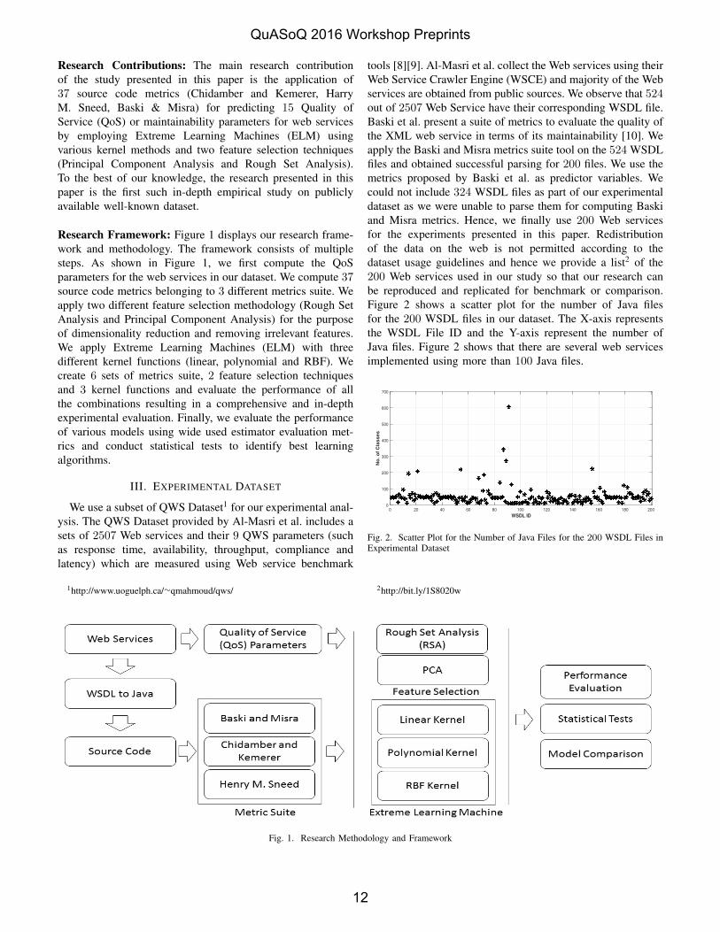
Research Framework: Figure 1 displays our research frame-work and methodology. The framework consists of multiplesteps. As shown in Figure 1, we first compute the QoSparameters for the web services in our dataset. We compute 37source code metrics belonging to 3 different metrics suite. Weapply two different feature selection methodology (Rough SetAnalysis and Principal Component Analysis) for the purposeof dimensionality reduction and removing irrelevant features.We apply Extreme Learning Machines (ELM) with threedifferent kernel functions (linear, polynomial and RBF). Wecreate 6 sets of metrics suite, 2 feature selection techniquesand 3 kernel functions and evaluate the performance of allthe combinations resulting in a comprehensive and in-depthexperimental evaluation. Finally, we evaluate the performanceof various models using wide used estimator evaluation met-rics and conduct statistical tests to identify best learningalgorithms.

III. EXPERIMENTAL DATASET

We use a subset of QWS Dataset1 for our experimental anal-ysis. The QWS Dataset provided by Al-Masri et al. includes asets of 2507 Web services and their 9 QWS parameters (suchas response time, availability, throughput, compliance andlatency) which are measured using Web service benchmark

1http://www.uoguelph.ca/∼qmahmoud/qws/

tools [8][9]. Al-Masri et al. collect the Web services using theirWeb Service Crawler Engine (WSCE) and majority of the Webservices are obtained from public sources. We observe that 524out of 2507 Web Service have their corresponding WSDL file.Baski et al. present a suite of metrics to evaluate the quality ofthe XML web service in terms of its maintainability [10]. Weapply the Baski and Misra metrics suite tool on the 524 WSDLfiles and obtained successful parsing for 200 files. We use themetrics proposed by Baski et al. as predictor variables. Wecould not include 324 WSDL files as part of our experimentaldataset as we were unable to parse them for computing Baskiand Misra metrics. Hence, we finally use 200 Web servicesfor the experiments presented in this paper. Redistributionof the data on the web is not permitted according to thedataset usage guidelines and hence we provide a list2 of the200 Web services used in our study so that our research canbe reproduced and replicated for benchmark or comparison.Figure 2 shows a scatter plot for the number of Java filesfor the 200 WSDL files in our dataset. The X-axis representsthe WSDL File ID and the Y-axis represent the number ofJava files. Figure 2 shows that there are several web servicesimplemented using more than 100 Java files.

WSDL ID

0 20 40 60 80 100 120 140 160 180 200

No

. o

f C

las

se

s

0

100

200

300

400

500

600

700

Fig. 2. Scatter Plot for the Number of Java Files for the 200 WSDL Files inExperimental Dataset

2http://bit.ly/1S8020w

Fig. 1. Research Methodology and Framework


12

IV. DEPENDENT VARIABLES QOS PARAMETERS

Table I shows the descriptive statistics of 9 QoS param-eters provided by the creators of QWS dataset. The ownersof QWS dataset provide QoS parameter values for all the2507 web services. However, Table I displays the descriptivestatistics computed by us for the 200 web services used inour experimental dataset. Table I reveals substantial variationor dispersion in the parameter values across 200 web serviceswhich shows variability in the quality across services. Sneedet al. describes a tool supported method for measuring webservice interfaces [11]. The extended version of their tool canbe used to compute maintainability, modularity, reusability,testability, interoperability and conformity of web services. Wecalculate these values for the 200 web services in our datasetand assign them as dependent variables. Table II displaysthe descriptive statistics for the QoS parameters calculatedusing Sneed’s Tool. Hence, we have a total of 15 dependentvariables.

TABLE IDESCRIPTIVE STATISTICS OF QOS PARAMETERS PROVIDED BY QWS

DATASET

Parameter Min Max Mean Median Std Dev Skewness KurtosisResponse Time 57.00 1664.62 325.11 252.20 289.33 3.15 13.12Availability 13.00 100.00 86.65 89.00 12.57 -2.63 12.06Throughput 0.20 36.90 7.04 4.00 6.94 1.57 5.79Successability 14.00 100.00 90.19 96.00 13.61 -2.57 10.81Reliability 33.00 83.00 66.64 73.00 9.61 -0.60 2.96Compliance 67.00 100.00 92.19 100.00 9.78 -0.90 2.61Best Practices 57.00 93.00 78.81 82.00 7.70 -0.68 2.67Latency 0.74 1337.00 42.81 12.20 106.23 9.56 112.68Documentation 1.00 96.00 29.37 32.00 26.97 1.06 3.31

TABLE IIDESCRIPTIVE STATISTICS OF QOS PARAMETERS CALCULATED USING

SNEEDS TOOL

Parameter Min Max Mean Median Std Dev Skewness KurtosisMaintainability 0.00 77.67 31.07 28.17 24.29 0.37 2.02Modularity 0.10 0.81 0.22 0.17 0.13 2.02 7.10Reusability 0.10 0.90 0.38 0.35 0.17 0.32 2.94Testability 0.10 0.66 0.19 0.16 0.09 2.58 10.71Interoperability 0.14 0.90 0.51 0.41 0.23 0.65 2.01Conformity 0.43 0.98 0.79 0.87 0.15 -0.47 1.57

V. PREDICTOR VARIABLES - SOURCE CODE METRICS

Chidamber and Kemerer Metrics: We compute severalsize and structure software metrics from the bytecode ofthe compiled Java files in our experimental dataset usingCKJM extended3 [12][13]. CKJM extended is an extendedversion of tool for calculating Chidamber and Kemerer JavaMetrics and many other metrics such as weighted methods perclass, coupling between object classes, lines of code, measureof functional abstraction, average method complexity andMcCabe’s Cyclomatic Complexity. We use the WSDL2JavaAxis2 code generator4 which comes built-in with an Eclipseplug-in to generate Java class files from the 200 WSDL filesin our experimental dataset. We then compile the Java files

3http://gromit.iiar.pwr.wroc.pl/p inf/ckjm/4https://axis.apache.org/axis2/java/core/tools/eclipse/wsdl2java-plugin.html

to generate the bytecode for computing the size and structuresoftware metrics using the CKJM extended tool. The minimumnumber of Java files are 7 and the maximum is 605. The mean,median, standard deviation, skewness and kurtosis is 52.39,45.50, 59.06, 5.43 and 43.94 respectively. Table III displaysthe descriptive statistics for 19 size and structure softwaremetrics computed using CKJM Extended Tool for the 200 Webservices in our dataset. The mean value of AMC as 61.94means that the mean of the average method size calculatedin terms of the number of Java binary codes in the methodfor each class is 62. We compute the standard deviation forall the 19 metrics to quantify the amount of dispersion andspread in the values. We observe (refer to Table III) that fewmetrics such as DIT, NOC, MFA, CAM, IC and CBM havelow standard deviation which means that the data points areclose to the mean. However, we observe that LCOM, LCO,AMC and CC have relatively high values of standard deviationwhich means that the data points are dispersed over a widerrange of values.

TABLE IIIDESCRIPTIVE STATISTICS OF OBJECT-ORIENTED METRICS

Metrics Min Max Mean Median Std Dev Skewness KurtosisWMC 9.48 13.57 11.01 10.96 0.48 0.81 6.54DIT 0.87 1.02 0.98 0.98 0.02 -2.07 9.72NOC 0.00 0.13 0.01 0.01 0.02 2.64 12.55CBO 4.10 12.55 10.70 11.01 1.33 -1.15 5.18RFC 12.78 44.55 40.35 41.48 4.13 -3.13 15.15LCOM 74.03 405.49 120.94 108.67 45.70 2.99 13.96Ca 0.64 3.92 2.91 2.99 0.62 -0.50 2.72Ce 3.49 9.50 8.24 8.37 0.90 -1.30 6.01NPM 4.88 9.27 6.55 6.47 0.48 1.07 7.90LCOM3 1.18 1.50 1.32 1.31 0.06 0.27 2.75LCO 76.14 493.64 399.18 411.50 54.03 -2.61 11.71DAM 0.21 0.45 0.37 0.37 0.04 -0.45 4.53MOA 0.02 2.28 0.60 0.53 0.28 2.00 11.03MFA 0.00 0.02 0.00 0.00 0.00 1.92 8.43CAM 0.39 0.43 0.40 0.40 0.01 0.22 4.54IC 0.00 0.05 0.01 0.01 0.01 0.79 3.68CBM 0.00 0.05 0.01 0.01 0.01 0.79 3.68AMC 7.68 82.86 61.94 64.37 10.75 -1.69 6.97CC 18.17 71.39 42.77 43.74 9.58 -0.29 3.67

TABLE IVDESCRIPTIVE STATISTICS OF HARRY M. SNEED’S METRICS SUITE

Metrics Min Max Mean Median Std Dev Skewness KurtosisData Complexity 0.10 0.81 0.28 0.27 0.17 0.60 2.59Relation Complexity 0.10 0.90 0.87 0.90 0.07 -7.72 83.58Format Complexity 0.14 0.72 0.60 0.64 0.09 -1.05 5.24Structure Complexity 0.15 0.90 0.61 0.63 0.17 -0.13 2.63Data Flow Complexity 0.10 0.90 0.87 0.90 0.10 -5.64 39.14Language Complexity 0.16 0.88 0.61 0.56 0.21 0.03 1.78Object Point 42.00 4581.00 299.32 200.00 483.31 5.67 41.67Data Point 29.00 3124.00 222.75 152.00 347.48 5.16 34.85Function Point 6.00 776.00 53.73 32.00 94.21 5.36 35.33Major Rule Violation 2.00 109.00 26.39 10.00 26.13 0.62 1.97Medium Rule Violation 2.00 16.00 5.02 5.00 1.94 0.56 6.71Minor Rule Violation 2.00 586.00 49.51 35.50 63.14 4.26 30.60

Harry M. Sneed Metrics: Sneed’s tool implements metricsfor quantity, quality and complexity of web service interfaces.The values of all the metrics are statically computed from aservice interface in WSDL as the suite of metrics is based onthe WSDL schema element occurrences [11]. We computesix interface complexity metrics for all the 200 web servicesin our dataset. The six interface complexity metrics arecomputed between a scale of 0.0 to 1.0. A value between 0.0


13

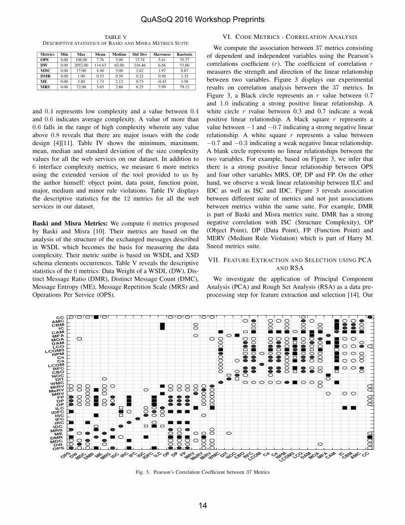
TABLE VDESCRIPTIVE STATISTICS OF BASKI AND MISRA METRICS SUITE

Metrics Min Max Mean Median Std Dev Skewness KurtosisOPS 0.00 108.00 7.76 5.00 13.74 5.41 35.37DW 0.00 2052.00 114.63 62.00 216.46 6.56 53.80MDC 0.00 17.00 4.40 5.00 2.62 1.97 8.87DMR 0.00 1.00 0.53 0.50 0.22 0.50 3.32ME 0.00 3.80 1.73 2.12 0.73 -0.43 3.58MRS 0.00 72.00 3.65 2.60 6.25 7.99 79.12

and 0.4 represents low complexity and a value between 0.4and 0.6 indicates average complexity. A value of more than0.6 falls in the range of high complexity wherein any valueabove 0.8 reveals that there are major issues with the codedesign [4][11]. Table IV shows the minimum, maximum,mean, median and standard deviation of the size complexityvalues for all the web services on our dataset. In addition to6 interface complexity metrics, we measure 6 more metricsusing the extended version of the tool provided to us bythe author himself: object point, data point, function point,major, medium and minor rule violations. Table IV displaysthe descriptive statistics for the 12 metrics for all the webservices in our dataset.

Baski and Misra Metrics: We compute 6 metrics proposedby Baski and Misra [10]. Their metrics are based on theanalysis of the structure of the exchanged messages describedin WSDL which becomes the basis for measuring the datacomplexity. Their metric suitbe is based on WSDL and XSDschema elements occurrences. Table V reveals the descriptivestatistics of the 6 metrics: Data Weight of a WSDL (DW), Dis-tinct Message Ratio (DMR), Distinct Message Count (DMC),Message Entropy (ME), Message Repetition Scale (MRS) andOperations Per Service (OPS).

VI. CODE METRICS - CORRELATION ANALYSIS

We compute the association between 37 metrics consistingof dependent and independent variables using the Pearson’scorrelations coefficient (r). The coefficient of correlation rmeasures the strength and direction of the linear relationshipbetween two variables. Figure 3 displays our experimentalresults on correlation analysis between the 37 metrics. InFigure 3, a Black circle represents an r value between 0.7and 1.0 indicating a strong positive linear relationship. Awhite circle r rvalue between 0.3 and 0.7 indicate a weakpositive linear relationship. A black square r represents avalue between −1 and −0.7 indicating a strong negative linearrelationship. A white square r represents a value between−0.7 and −0.3 indicating a weak negative linear relationship.A blank circle represents no linear relationships between thetwo variables. For example, based on Figure 3, we infer thatthere is a strong positive linear relationship between OPSand four other variables MRS, OP, DP and FP. On the otherhand, we observe a weak linear relationship between ILC andIDC as well as ISC and IDC. Figure 3 reveals associationbetween different suite of metrics and not just associationsbetween metrics within the same suite. For example, DMRis part of Baski and Misra metrics suite. DMR has a strongnegative correlation with ISC (Structure Complexity), OP(Object Point), DP (Data Point), FP (Function Point) andMERV (Medium Rule Violation) which is part of Harry M.Sneed metrics suite.

VII. FEATURE EXTRACTION AND SELECTION USING PCAAND RSA

We investigate the application of Principal ComponentAnalysis (PCA) and Rough Set Analysis (RSA) as a data pre-processing step for feature extraction and selection [14]. Our

OPS

DW

MDC

DMR

ME

MRS

IDC

IRC

IFC

ISCID

FCIL

C OP DP FP

MRV

MeRV

MiR

V

WM

CDIT

NOCCBO

RFC

LCOM Ca Ce

NPM

LCOM

3LCO

DAMM

OAM

FACAM IC

CBMAM

C CC

OPSDW

MDC DMR

ME MRS IDC IRCIFCISC

IDFCILCOPDPFP

MRVMeRVMiRVWMC

DITNOCCBORFC

LCOMCaCe

NPMLCOM3

LCODAMMOAMFACAM

ICCBMAMC

CC

Fig. 3. Pearson’s Correlation Coefficient between 37 Metrics


14

objective behind using PCA and RSA is to identify featureswhich are relevant in-terms of high predictive power andimpact on the dependent variable and filter irrelevant featureswhich have little or no impact on the classifier accuracy [14].We apply PCA and varimax rotation method on all sourcecode metrics. The experimental results of PCA analysis isshown in Table VI. Table VI reveals the relationship betweenthe original source code metrics and the domain metrics. Foreach PC (Principal Components), we provide the eigenvalue,variance percent, cumulative percent and source code metricsinterpretation (refer to Table VI). In PCA the order of theeigenvalues from highest to lowest indicates the principalcomponents in the order of significance. Among all PrincipalComponents, we select only those which have Eigen valuegreater than 1. Our analysis reveals that 9 PCs have Eigenvalue greater than 1 (refer to Table VI). Table VI shows themapping of each component to the most important metric forthat component. Table VII shows the optimal subset of featuresfor every dependent variable derived from the original set of37 source code metrics based features after applying RSA. Weapply the RSA procedure 15 times (one for each dependentvariable). Table VII reveals that it is possible to reduce thenumber of features substantially and several features from theoriginal set are found to be uncorrelated.

TABLE VIFEATURE EXTRACTION USING PRINCIPAL COMPONENT ANALYSIS -

DESCRIPTIVE STATISTICS

PC Eigenvalue % variance Cumulative % Metrics InterpretationPC1 6.4 17.3 17.3 CBO, RFC, Ca, Ce, LCOM3, LCO, DAM, CAMPC2 5.8 15.76 33.06 OPS, MRS, IRC, IDFC, OP, DP, FPPC3 3.67 9.94 43.00 DW, MDC, MeRV, MiRV, CC, MEPC4 3.39 9.16 52.17 DMR, IDC,ISC, ILCPC5 3.34 9.03 61.2 IC, CBM, MOAPC6 2.5 6.77 67.98 IFC, DIT, NOC, MFAPC7 2.23 6.02 74.00 WMC, NPMPC8 2.14 5.79 79.79 MRV, AMCPC9 1.36 3.7 83.5 LCOM

TABLE VIISOURCE CODE METRICS (FEATURE) SELECTION OUTPUT USING ROUGH

SET ANALYSIS (RSA)

QoS Selected MetricsResponse Time DMR, SC, LC, WMC, Ca, LCOM3, MFA, CAM, IC, CCAvailability FC, SC, LC, MeRV, MiRV, WMC, Ca, LCOM3, MFA, CAM, IC, CCThroughput ME, FC, SC, LC, MRV, MeRV, MiRV, Ce, MOA, MFA, CAM, CBM, CCSuccessability ME, FC, SC, DFC, LC, MRV, WMC, LCOM3, LCO, DAM, MOA, CAMReliability FC, SC, DFC, LC, WMC, LCOM3, LCO, MOA, MFA, CAM, CBMCompliance ME, FC, SC, DFC, LC, MRV, WMC, MiRV, Ca, CC, DAM, MOA, CAM, NPMBest Practices ME, FC, SC, DFC, LC, MRV, MiRV, WMC, Ca, NPM, MOA, MFA, CAM, CCLatency DMR, ME, DC, FC, DFC, LC, MRV, NOC, NPM, LCO, MOA, CAM, ICDocumentation ME, FC, SC, DFC, LC, MRV, MeRV, WMC, Ca, NPM, CAM, IC, CCMaintainability DP, Ce, LCOM3, MOA, MFA, CAM, CBMModularity DMR, ME, SC, DFC, LC, DP, MRV, MiRV, WMC, Ca, MOA, IC, AMCReusability MDC, DMR, FC, SC, DFC, LC, LCOM, LCOM3Testability ME, FC, SC, LC, MiRV, DIT, NOC, CC, RFCInteroperability SC, LC, MeRV, MiRV, WMC, DIT, CBO, MFA, CCConformity ME, FC, DFC, LC, MRV, WMC, Ca, CAM

VIII. APPLICATION OF EXTREME LEARNING MACHINES(ELMS)

Huan et al. mention that Extreme Learning Machines(ELMs) have shown to outperform computational intelligencetechniques such as Artificial Neural Networks (ANNs) and

Support Vector Machines (SVMs) in-terms of learning speedand computational scalability [15]. ELM has demonstratedgood potential to resolving regression and classification prob-lems [15] and our objective is to investigate if ELMs canbe successfully applied in the domain of web service QoSprediction using source code metrics. Selection of an appro-priate kernel function depending on the application domainand dataset is an important and core issue [16].

Ding et al. mention that there is a correlation betweenthe generalization performance and learning performance withthe kernel function [16] as in the case of traditional neuralnetworks [16]. Hence, we investigate the performance of theELM based classifier using three different kernel functions:linear, polynomial and RBF. ELMs can be used with differentkernel functions and one can create hybrid kernel functionsalso. The most basic, simplest and fastest is the linear ker-nel function which is used as a baseline for comparisonwith more complicated kernel functions such as polynomialand RBF. Table VIII shows the performance of the ELMbased classifier with linear kernel function. Table IX showsthe performance of the ELM based predictive model withsecond degree polynomial kernel. The polynomial kernel ismore sophisticated than the linear kernel and uses non-linearequations instead of the linear equations for the purpose ofregression and classification and is expected to result in betteraccuracy in comparison to the classifier with linear kernel. TheRadial Basis Function kernel (RBF or Gaussian) is a popularkernel function and widely used in Support Vector Machine(SVM) learning algorithm. We use linear kernel to investigateif the data is linearly separable but also use polynomial andRBF kernel to examine if our data is not linearly separable(computing a non-linear decision boundary). We employ fourdifferent performance metrics (MAE, MMRE, RMSE and r-value) to study the accuracy of the classifiers. The MeanAbsolute Error (MAE) measures the difference between thepredicted or forecasted value and the actual values (averageof the absolute errors). Table VIII and IX reveals that theforecast for several predictive model is very accurate as theMAE value is less than 0.05. For example, the MAE valuefor HMS, AM and PCA metrics for predicting Conformity is0.03. Table VIII and IX reveals that in general the predictiveaccuracy for response time, latency, modularity and conformityis better than the predictive accuracy of other QoS parameters.

Kitchenham et al. mention that Mean Magnitude of RelativeError (MMRE) is a widely used assessment criterion forevaluating the predictive accuracy and overall performanceof competing software prediction models and particularlythe software estimation models [17]. MMRE computes thedifference between actual and predicted value relative to theactual value. Table X shows that the MMRE values for ELMwith RBF kernel is between 0.30 to 0.35 for response time,availability and successability and indicates good estimationability of the classifier. Table VIII and Table IX revealsthat the MMRE values for conformity QoS parameter areas low as 0.05, 0.06, 0.10 and 0.11. Root Mean SquareError (RMSE) or Root Mean square Deviation root-mean-


15

TABLE VIIIPERFORMANCE MATRIX FOR ELM WITH LINEAR KERNEL

Respon

seTim

e

Availa

bility

Throu

ghpu

t

Succ

essab

ility

Reliab

ility

Compli

ance

BestPra

ctice

s

Latenc

y

Docum

entat

ion

Main

taina

bility

Mod

ularit

y

Reusa

bility

Testa

bility

Inter

oper

abilit

y

Confor

mity

MAEBMS 0.11 0.19 0.18 0.21 0.25 0.28 0.19 0.11 0.23 0.20 0.11 0.16 0.12 0.16 0.18HMS 0.10 0.16 0.18 0.19 0.25 0.27 0.19 0.11 0.22 0.15 0.08 0.15 0.07 0.14 0.06OOM 0.09 0.14 0.18 0.17 0.25 0.25 0.18 0.11 0.22 0.12 0.15 0.15 0.14 0.22 0.18AM 0.10 0.15 0.18 0.18 0.26 0.27 0.20 0.11 0.21 0.11 0.07 0.13 0.06 0.11 0.06PCA 0.10 0.16 0.19 0.18 0.26 0.26 0.21 0.12 0.21 0.16 0.09 0.14 0.10 0.14 0.09RSA 0.11 0.17 0.18 0.20 0.25 0.26 0.19 0.11 0.23 0.27 0.16 0.17 0.15 0.25 0.26

MMREBMS 0.37 0.35 0.73 0.38 0.66 0.61 0.37 0.55 0.90 0.76 0.41 0.61 0.46 0.35 0.28HMS 0.36 0.33 0.73 0.36 0.69 0.61 0.39 0.56 0.93 0.60 0.29 0.60 0.26 0.31 0.11OOM 0.34 0.32 0.74 0.35 0.71 0.61 0.37 0.55 0.89 0.47 0.54 0.57 0.55 0.50 0.33AM 0.36 0.34 0.71 0.37 0.71 0.64 0.47 0.54 0.90 0.42 0.22 0.46 0.20 0.25 0.10PCA 0.34 0.34 0.74 0.36 0.69 0.59 0.49 0.60 0.88 0.60 0.30 0.59 0.37 0.33 0.16RSA 0.36 0.34 0.71 0.37 0.69 0.57 0.36 0.54 0.88 1.09 0.60 0.67 0.54 0.52 0.44

RMSEBMS 0.16 0.26 0.22 0.28 0.29 0.33 0.24 0.15 0.29 0.26 0.17 0.22 0.17 0.22 0.22HMS 0.15 0.22 0.22 0.24 0.29 0.31 0.23 0.15 0.28 0.21 0.12 0.19 0.11 0.18 0.08OOM 0.15 0.21 0.22 0.23 0.29 0.30 0.22 0.14 0.28 0.16 0.22 0.19 0.21 0.28 0.23AM 0.15 0.22 0.22 0.24 0.29 0.32 0.24 0.14 0.27 0.14 0.11 0.16 0.10 0.15 0.08PCA 0.15 0.22 0.22 0.25 0.29 0.31 0.25 0.16 0.27 0.21 0.13 0.20 0.14 0.19 0.13RSA 0.17 0.26 0.22 0.29 0.30 0.31 0.23 0.14 0.29 0.34 0.22 0.23 0.21 0.31 0.32

r-valueBMS 0.34 0.30 0.30 0.45 0.50 0.49 0.47 0.45 0.41 0.84 0.81 0.50 0.90 0.88 0.79HMS 0.35 0.33 0.39 0.38 0.21 0.28 0.62 0.21 0.23 0.88 0.90 0.83 0.94 0.88 0.98OOM 0.66 0.62 0.57 0.27 0.65 0.48 0.64 0.48 0.33 0.94 0.74 0.78 0.51 0.67 0.77AM 0.32 0.35 0.37 0.26 0.34 0.30 0.34 0.58 0.27 0.94 0.98 0.90 0.93 0.92 0.99PCA 0.40 0.32 0.37 0.39 0.41 0.40 0.29 0.36 0.37 0.87 0.94 0.79 0.86 0.90 0.99RSA 0.29 0.77 0.49 0.45 0.37 0.48 0.55 0.31 0.43 0.11 0.36 0.48 0.70 0.77 0.43

TABLE IXPERFORMANCE MATRIX FOR ELM WITH POLYNOMIAL KERNEL

Respon

seTim

e

Availa

bility

Throu

ghpu

t

Succ

essab

ility

Reliab

ility

Compli

ance

BestPra

ctice

s

Latenc

y

Docum

entat

ion

Main

taina

bility

Mod

ularit

y

Reusa

bility

Testa

bility

Inter

oper

abilit

y

Confor

mity

BMS 0.10 0.14 0.18 0.17 0.24 0.26 0.19 0.11 0.23 0.17 0.11 0.16 0.11 0.15 0.12HMS 0.11 0.15 0.19 0.17 0.26 0.28 0.19 0.11 0.23 0.12 0.05 0.11 0.04 0.10 0.03OOM 0.12 0.15 0.21 0.18 0.27 0.28 0.19 0.11 0.23 0.12 0.13 0.14 0.15 0.18 0.12AM 0.13 0.20 0.20 0.23 0.28 0.33 0.23 0.13 0.28 0.10 0.06 0.12 0.05 0.11 0.03PCA 0.11 0.15 0.20 0.18 0.24 0.26 0.19 0.12 0.23 0.10 0.06 0.13 0.07 0.11 0.03RSA 0.10 0.14 0.18 0.16 0.24 0.26 0.18 0.11 0.22 0.25 0.14 0.16 0.14 0.23 0.23



r-valueBMS 0.46 0.30 0.39 0.16 0.36 0.16 0.38 0.07 0.09 0.86 0.88 0.45 0.93 0.89 0.89HMS 0.18 0.31 0.19 0.38 -0.02 0.19 0.24 0.46 0.37 0.94 0.97 0.90 1.00 0.95 1.00OOM 0.08 0.29 0.38 0.22 0.36 0.16 0.34 0.42 0.46 0.96 0.77 0.72 0.59 0.75 0.92AM 0.12 0.31 0.40 -0.01 0.40 0.19 0.42 0.50 0.37 0.95 0.99 0.91 0.98 0.94 1.00PCA 0.18 -0.04 0.46 0.19 0.29 0.39 0.58 0.51 0.51 0.94 0.98 0.90 0.99 0.95 1.00RSA 0.25 0.37 0.54 0.26 0.39 0.24 0.42 0.13 0.26 0.60 0.75 0.45 0.51 0.70 0.62

square deviation computes the sample standard deviation ofthe differences between predicted values by the estimator andactual values. RMSE is also an indicator of the predictedand observed values. From Table VIII, we infer that the bestRMSE value in-case of ELM with linear kernel is for responsetime and latency QoS parameters. The minimum RMSE valueobtained is 0.08 for HMS metrics and conformity parameterin-case of linear kernel. From Table VIII, we observe thatin-case of polynomial kernel, the performance of PCA basedfeature extraction technique is better for some parameters incomparison to RSA based feature selection technique andsimilarly the performance of RSA is better than PCA for some

parameters. We do not observe a dominate approach betweenPCA and RSA.

IX. COMPARING ALGORITHMS USING STATISTICALSIGNIFICANCE TESTING

Our objective is to compare several learning algorithms andassess which algorithm is better. Dietterich et al. review 5 ap-proximate statistical tests for determining whether one learningalgorithm outperforms another on a particular learning taskand dataset [18]. We apply the 10-fold cross-validated paired t-test as described in the paper by Dietterich et al. [18]. We haveseveral combination of subsets of metrics and ELM kernelfunctions as learning algorithms. We consider 6 different sets


16

TABLE XPERFORMANCE MATRIX FOR ELM WITH RBF KERNEL

Respon

seTim

e

Availa

bility

Throu

ghpu

t

Succ

essab

ility

Reliab

ility

Compli

ance

BestPra

ctice

s

Latenc

y

Docum

entat

ion

Main

taina

bility

Mod

ularit

y

Reusa

bility

Testa

bility

Inter

oper

abilit

y

Confor

mity

BMS 0.10 0.14 0.18 0.17 0.24 0.26 0.18 0.11 0.22 0.25 0.16 0.16 0.14 0.24 0.25HMS 0.10 0.14 0.18 0.17 0.24 0.26 0.18 0.11 0.22 0.25 0.16 0.18 0.14 0.25 0.29OOM 0.09 0.13 0.18 0.16 0.24 0.25 0.18 0.11 0.22 0.24 0.17 0.16 0.15 0.25 0.27AM 0.09 0.13 0.19 0.17 0.24 0.26 0.20 0.11 0.21 0.24 0.17 0.17 0.14 0.24 0.31PCA 0.09 0.13 0.19 0.16 0.24 0.25 0.20 0.11 0.21 0.24 0.17 0.17 0.14 0.24 0.30RSA 0.10 0.13 0.18 0.16 0.24 0.25 0.18 0.11 0.22 0.26 0.16 0.16 0.14 0.26 0.26



r-valueBMS 0.31 0.50 0.19 0.02 0.08 0.24 0.50 0.46 0.15 0.87 0.81 0.47 0.81 0.78 0.93HMS 0.34 0.18 0.43 0.38 0.29 0.33 0.33 0.38 0.34 0.93 0.96 0.48 0.91 0.78 0.97OOM 0.57 0.34 0.35 0.44 0.55 0.37 0.64 0.29 0.26 0.82 0.58 0.71 0.53 0.70 0.83AM 0.63 0.39 0.29 0.20 0.48 0.28 0.32 0.30 0.34 0.96 0.94 0.62 0.83 0.91 0.95PCA 0.50 0.20 0.32 0.00 0.44 0.41 0.64 0.26 0.24 0.92 0.73 0.68 0.75 0.85 0.98RSA 0.21 0.39 0.36 0.42 0.38 0.46 0.61 0.35 0.43 0.42 0.59 0.20 0.44 0.56 0.57

of metrics: All Metrics (AM), Only Object Oriented Metrics(OOM), Harry M. Sneed’s Metrics (HMS), Baski and MisraMetrics (BMS), Metrics derived after executing PCA, andmetrics derived after executing RSA. We consider 6 sets ofmetrics as input to develop a model to predict 15 differentQoS parameters. We investigate the application of extremelearning machine with three different types of kernel functions:linear kernel, polynomial kernel, and radial basis functionwith three different performance parameters. Hence, for each

subset of metrics, a total number of three set (one for eachperformance measure) are used, each with 45 data points (3kernels multiplied by 15 QoS parameters). Table XI displaysthe result of the 10-fold cross-validated paired t-test analysis.For each of the 3 kernels (Linear, Polynomial and RBF),6 different subset of metrics are considered as input withthree different performance parameters. The three differentperformance parameters are: Mean Absolute Error (MAE),Mean Magnitude of Relative Error (MMRE) and Root Mean

TABLE XIEXPERIMENTAL RESULTS ON T-TEST BETWEEN DIFFERENT SET OF METRICS

MAEMean Difference p-value

BMS HMS OOM AM PCA RSA BMS HMS OOM AM PCA RSABMS 0.000 0.014 0.000 0.009 0.011 -0.013 NaN 0.004 0.986 0.140 0.008 0.008HMS -0.014 0.000 -0.014 -0.004 -0.002 -0.026 0.004 NaN 0.017 0.164 0.175 0.003OOM 0.000 0.014 0.000 0.009 0.011 -0.013 0.986 0.017 NaN 0.155 0.025 0.026AM -0.009 0.004 -0.009 0.000 0.002 -0.022 0.140 0.164 0.155 NaN 0.570 0.035PCA -0.011 0.002 -0.011 -0.002 0.000 -0.024 0.008 0.175 0.025 0.570 NaN 0.005RSA 0.013 0.026 0.013 0.022 0.024 0.000 0.008 0.003 0.026 0.035 0.005 NaN

MMREMean Difference p-value

BMS HMS OOM AM PCA RSA BMS HMS OOM AM PCA RSABMS 0.000 0.037 0.000 0.026 0.027 -0.037 NaN 0.011 0.990 0.182 0.051 0.009HMS -0.037 0.000 -0.037 -0.010 -0.010 -0.074 0.011 NaN 0.039 0.346 0.199 0.005OOM 0.000 0.037 0.000 0.026 0.027 -0.037 0.990 0.039 NaN 0.199 0.081 0.078AM -0.026 0.010 -0.026 0.000 0.000 -0.063 0.182 0.346 0.199 NaN 0.967 0.048PCA -0.027 0.010 -0.027 0.000 0.000 -0.064 0.051 0.199 0.081 0.967 NaN 0.014RSA 0.037 0.074 0.037 0.063 0.064 0.000 0.009 0.005 0.078 0.048 0.014 NaN

RMSEMean Difference p-value

BMS HMS OOM AM PCA RSA BMS HMS OOM AM PCA RSABMS 0.000 0.018 -0.001 0.010 0.013 -0.014 NaN 0.002 0.781 0.205 0.008 0.005HMS -0.018 0.000 -0.020 -0.008 -0.005 -0.033 0.002 NaN 0.010 0.066 0.038 0.002OOM 0.001 0.020 0.000 0.012 0.014 -0.013 0.781 0.010 NaN 0.167 0.021 0.050AM -0.010 0.008 -0.012 0.000 0.003 -0.025 0.205 0.066 0.167 NaN 0.575 0.045PCA -0.013 0.005 -0.014 -0.003 0.000 -0.027 0.008 0.038 0.021 0.575 NaN 0.004RSA 0.014 0.033 0.013 0.025 0.027 0.000 0.005 0.002 0.050 0.045 0.004 NaN


17

TABLE XIIEXPERIMENTAL RESULTS ON T-TEST BETWEEN THREE DIFFERENT KERNELS

Mean DifferenceMAE MRE RMSE

Linear Polynomial RBF Linear Polynomial RBF Linear Polynomial RBFLinear 0.000 0.007 -0.021 Linear 0.000 0.005 -0.084 Linear 0.000 0.005 -0.018Polynomial -0.007 0.000 -0.028 Polynomial -0.005 0.000 -0.090 Polynomial -0.005 0.000 -0.023RBF 0.021 0.028 0.000 RBF 0.084 0.090 0.000 RBF 0.018 0.023 0.000

p-valueMAE MRE RMSE

Linear Polynomial RBF Linear Polynomial RBF Linear Polynomial RBFLinear NaN 0.13 0.001 Linear NaN 0.467 0.000 Linear NaN 0.121 0.007Polynomial 0.13 NaN 0.000 Polynomial 0.467 NaN 0.000 Polynomial 0.121 NaN 0.005RBF 0.001 0.000 NaN RBF 0.000 0.000 NaN RBF 0.007 0.005 NaN

Squared Error (RMSE). Hence for each kernel a total three set(one for each performance measure) are used, each with 90data points (six subsets of metrics multiplied by 15 QoS). Theexperimental results of t-test analysis for different performanceparameter (MAE, MMRE and RMSE) and three different ELMkernels are summarized in Table XII. Table XII contains twoparts. The first part of the table XII shows the mean differencevalue and second part shows the p-value between differentpairs. Table XII reveals that there is no significant differencebetween the kernel function, due to the fact that p-value isgreater than 0.05. However, by closely examining the valueof mean difference, polynomial kernel yields better resultcompared to other kernels function i.e., linear and RBF kernelfunctions.

X. CONCLUSION

We develop a predictive model to estimate QoS parametersof web services using source code (implementing the services)metrics. We experiment with six different sets of metrics asinput to develop a prediction model. The performance of thesesets of metrics are evaluated using Extreme Learning Machines(ELM) with various kernel functions such as linear, polyno-mial and RBF kernel function. From the correlation analysisbetween metrics, we observe that there exists a high correlationbetween Object-Oriented metrics and WSDL metrics. From t-test analysis, we infer that in most of the cases, there is thedifference between the various sets of metrics in terms of theperformance of the estimator is not substantial but moderate.We observe that the predictive model developed using HarryM. Sneed (HMS) metrics yields better result compared to othersets of metrics such as all metrics and Baski and Misra metrics.From t-test analysis, we can also interpret that differencebetween the three kernel functions in-terms of their influenceon the predictive accuracy is moderate. We conclude that noneof the feature selection technique dominate the other and onefeature selection method is better than the other for someQoS parameters and vice-versa. By assessing the value ofmean difference, we infer that the polynomial kernel for ELMyields better result compared to other kernels function i.e.,linear and RBF kernel functions. From performance results,it is observed that the performance of the predictive modelor estimator varies with the different sets of software metrics,feature selection technique and the kernel functions. Finally,we conclude that it is possible to estimate the QoS parametersusing ELM and source code metrics.

REFERENCES

[1] F. Curbera, M. Duftler, R. Khalaf, W. Nagy, N. Mukhi, and S. Weer-awarana, “Unraveling the web services web: an introduction to soap,wsdl, and uddi,” IEEE Internet computing, vol. 6, no. 2, p. 86, 2002.

[2] E. Newcomer and G. Lomow, Understanding SOA with Web services.Addison-Wesley, 2005.

[3] J. L. O. Coscia, M. Crasso, C. Mateos, A. Zunino, and S. Misra,Predicting Web Service Maintainability via Object-Oriented Metrics:A Statistics-Based Approach. Springer Berlin Heidelberg, 2012, pp.29–39.

[4] J. L. O. Coscia, M. Crasso, C. Mateos, and A. Zunino, “Estimating webservice interface quality through conventional object-oriented metrics.”CLEI Electron. J., vol. 16, 2013.

[5] C. Mateos, M. Crasso, A. Zunino, and J. L. O. Coscia, “Detecting wsdlbad practices in code-first web services,” Int. J. Web Grid Serv., vol. 7,no. 4, pp. 357–387, Jan. 2011.

[6] L. Kumar, M. Kumar, and S. K. Rath, “Maintainability prediction of webservice using support vector machine with various kernel methods,” In-ternational Journal of System Assurance Engineering and Management,pp. 1–18, 2016.

[7] S. O. Olatunji, Z. Rasheed, K. Sattar, A. Al-Mana, M. Alshayeb, andE. El-Sebakhy, “Extreme learning machine as maintainability predictionmodel for object-oriented software systems,” Journal of Computing,vol. 2, no. 8, pp. 49–56, 2010.

[8] E. Al-Masri and Q. H. Mahmoud, “Qos-based discovery and rankingof web services,” in Computer Communications and Networks, 2007.ICCCN 2007. Proceedings of 16th International Conference on, 2007,pp. 529–534.

[9] E. Al Masri and Q. H. Mahmoud, “Investigating web services on theworld wide web,” Proceedings of the 17th International Conference onWorld Wide Web, pp. 795–804, 2008.

[10] D. Baski and S. Misra, “Metrics suite for maintainability of extensiblemarkup language web services,” IET Software, vol. 5, no. 3, pp. 320–341, 2011.

[11] H. M. Sneed, “Measuring web service interfaces,” in Web SystemsEvolution (WSE), 2010 12th IEEE International Symposium on, 2010,pp. 111–115.

[12] M. Jureczko and D. Spinellis, Using Object-Oriented Design Metricsto Predict Software Defects, ser. Monographs of System Dependability,2010, vol. Models and Methodology of System Dependability, pp. 69–81.

[13] D. Spinellis, “Tool writing: a forgotten art? (software tools),” IEEESoftware, vol. 22, no. 4, pp. 9–11, 2005.

[14] R. W. Swiniarski and A. Skowron, “Rough set methods in featureselection and recognition,” Pattern recognition letters, vol. 24, no. 6,pp. 833–849, 2003.

[15] G.-B. Huang, D. H. Wang, and Y. Lan, “Extreme learning machines:a survey,” International Journal of Machine Learning and Cybernetics,vol. 2, no. 2, pp. 107–122, 2011.

[16] S. Ding, Y. Zhang, X. Xu, and L. Bao, “A novel extreme learningmachine based on hybrid kernel function,” Journal of Computers, vol. 8,no. 8, pp. 2110–2117, 2013.

[17] B. A. Kitchenham, L. M. Pickard, S. G. MacDonell, and M. J. Shepperd,“What accuracy statistics really measure [software estimation],” IEEProceedings-Software, vol. 148, no. 3, pp. 81–85, 2001.

[18] T. G. Dietterich, “Approximate statistical tests for comparing supervisedclassification learning algorithms,” Neural Comput., vol. 10, no. 7, pp.1895–1923, Oct. 1998.


18

Local Variables with Compound Names andComments as Signs of Fault-Prone Java Methods

Hirohisa Aman

Center for Information TechnologyEhime University

Matsuyama, Ehime 790-8577, JapanEmail: [email protected]

Sousuke AmasakiTomoyuki Yokogawa

Faculty of Computer Scienceand Systems Engineering

Okayama Prefectural UniversitySoja, Okayama 719–1197, Japan

Minoru Kawahara

Center for Information TechnologyEhime University

Matsuyama, Ehime 790-8577, Japan

Abstract—This paper focuses on two types of artifacts—localvariables and comments in a method (function). Both of them areusually used at the programer’s discretion. Thus, naming localvariables and commenting code can vary among individuals, andsuch an individual difference may cause a dispersion in quality.This paper conducts an empirical analysis on the fault-pronenessof Java methods which are collected from nine popular opensource products. The results report the following three findings:(1) Methods having local variables with compound names aremore likely to be faulty than the others; (2) Methods havinglocal variables with simple and short names are unlikely to befaulty, but their positive effects tend to be decayed as their scopesget wider; (3) The presence of comments within a method bodycan also be useful sign of fault-prone method.

I. INTRODUCTION

Software systems have been utilized in many aspects of ourdaily life, and management of software quality has been themost significant activity for ensuring the safety and securityof the people. In fact, it is hard to always make a one-shotrelease of a perfect software product which has no need to beenhanced or modified in the future; software systems usuallyrequire upgrades after their releases in order to fix their faultsand/or to enrich their functionality. Needless to say, it is betterto reduce both the frequency of their upgrades and the size oftheir patches to be applied.

To minimize upgrades of software products, thorough re-view and testing before their releases are desirable activities.In general, software review and testing help to detect concealedfaults or identify suspicious software modules which are fault-prone [1], [2]. Then, those problems can be resolved by fixingfaults or refactoring problematic programs in order to reducethe risk of causing unwanted upgrades after their releases.While review and testing are useful activities, they are alsocostly ones, so there have been many studies using softwaremetrics to predict fault-prone modules prior to software reviewand testing activities [3]. By predicting fault-prone parts of asoftware product, cost-effective review and testing would beperformed, i.e., we would detect more faults at less cost.

Most studied methods and models for predicting fault-pronemodules have been based on structural features of productssuch as their sizes and complexities, or on development histo-

ries stored in their code repositories such as the number of bug-fix commitments which have been made by a certain point intime [4], [5], [6]. However, the impact of human factors wouldalso be significant since programming activities are usuallydone by human beings. Different programmers would probablydevelop different programs for the same specification. Sucha difference among individuals must have a certain level ofinfluence on the quality of products, i.e., it must cause adispersion in quality. Therefore, we focus on the followingtwo artifacts which may vary from person to person, (1) localvariables declared in a method (function) and (2) commentswritten inside the method body. While these artifacts have noimpact on the structure of a program, they seem to be relatedto the understandability and the readability of the program,so they can be expected to play important roles in predictingfault-prone methods. In this paper, we quantitatively analyzethe relationships of these artifacts with the fault-proneness.

The key contribution of this paper is to provide the follow-ing findings derived from the results of our empirical analysiswith nine popular open source software (OSS) products:

• Local variables with descriptive compound names (for ex-ample, “countOfSatisfactoryRecords”) can besigns that the methods are fault-prone.

• Methods having local variables with simple and shortnames (for example, “c” or “cnt”) are unlikely to befaulty, but their positive effects tend to be decayed astheir scopes get wider.

• Comments within a method body also seem to be relatedto the fault-proneness of the method.

The remainder of this paper is organized as follows. SectionII describes two types of artifacts which may vary amongprogrammers—(1) names of local variables and (2) commentswritten inside a method body—and their relationships with thequality of source programs, and gives our research questionsin regard to impacts of those artifacts. Section III reportson an empirical analysis on our research questions usingpopular OSS products, and discusses the results. Section IVbriefly describes related work. Finally, Section V presents theconclusion of this paper and our future work.


19

II. LOCAL VARIABLES AND COMMENTS

This paper focuses on local variables and comments, sincethey may vary widely from person to person and cause avariation in quality. This section describes concerns of localvariable names and comments in regard to source code quality,and set up our research questions.

A. Local Variable Name

Since local variables are valid only within a function ora method, names of local variables are usually not spec-ified in their software specifications or design documents.Therefore, naming local variables can be at the programmer’sdiscretion. In general, different programmers would preferdifferent names for local variables even if they implementthe same algorithm in their function or method. For example,a programmer likes to use “count” as the name of localvariable for storing the number of records which satisfy acertain condition, but another programmer prefers “c” as itsname; there might even be a programmer who wants to give“countOfSatisfactoryRecords” to the variable.

Needless to say, local variables with fully-spelled namessuch as “count” or ones with descriptive compound names“countOfSatisfactoryRecords” make it easy to un-derstand the roles of those variables in their function ormethod since those names provide more information aboutthose variables than shorter and/or simpler names. Lawrie etal. [7] surveyed the understandability of identifiers (includingnot only local variables’ names but also functions’ names)used in programs by comparing three types of names, (1)fully-spelled names such as “count,” (2) abbreviated namessuch as “cnt” and (3) names using only an initial lettersuch as “c.” They reported that a longer name is easier tounderstand for programmers, but there is not a significantdifference in comprehensibility between fully-spelled namesand abbreviated ones in their survey results. That is to say, itis not always necessary to give a long and descriptive name toa local variable, and a short and simple name may be sufficient.

There are also programming heuristics on naming localvariables. Both the GNU coding standards [8] and the Javacoding convention [9] have said that names of local variablesshould be shorter. Moreover, Kernighan and Pike [10] alsoargued that shorter names are sufficient for local variables;for example, they considered that name “n” looks good fora local variable storing “the number of points” while name“numberOfPoints” seems to be overdone. Thus, long anddescriptive names have not been recommended for the namesof local variables. However, the impact of such a descriptivename on the code quality has not been clearly discussed inthose heuristics.

Aman et al. [11] conducted an empirical work and showedthat methods having local variables with long names aremore likely to be fault-prone and change-prone than the othermethods. That is to say, they showed a relationship between along name of a local variable and a poor quality of the codein a statistical manner. However, their analysis missed takinginto account the following two aspects: (1) the composition of

variable’s name and (2) the scope of local variable. Focusingon not only the length of local variable’s name but also thosetwo aspects would be more worthy in analyzing the impactof local variable’s name and in enhancing the quality of code.This is a key motivation of this work.

B. Comments

Comments are documents embedded in a source file, whichusually provide beneficial information in regard to the program[12]. While there are several types of comments, we focuson comments written inside a method (function) body inthis paper. Those comments usually give explanations orprogrammer’s memos for their implementation in the method.Of course, the other types of comments also provide importantinformation regarding the program. However, such commentswritten outside a method body are often the copyright des-ignation or the programmer’s manual explaining how to usethe method, i.e., those comments may not be decided at thediscretion of the programmer. Thus, those comments outsidea method body may be out of our research scope focusingon the individual difference among programmers. That is thereason why we will focus only on the comments written insidea method body.

While comments along with executable code can be a greathelp in understanding the code, there have also been criticismson their effects: comments might be written to compensatefor a lack of readability in complicated programs [13]. In thiscontext, Fowler [14] pointed out that well-written commentsmay be “deodorant” for masking “code smells.” Althoughcomments themselves are good artifacts, they may be usedfor neutralizing a “bad-smelling” code. Kernighan and Pike[10] said that programmers should not add detailed commentsto a bad code; in such a case, it is better to rewrite theircode rather than adding comments. If a programmer wants toadd detailed comments to their code during their programmingactivity, the programmer may consider that the program ishard to understand for others without those comments. Thatis to say, comments may be signs of complicated programs.Aman et al. [11], [15] reported supporting empirical resultsthat commented programs tend to be more fault-prone thannon-commented ones. In this paper, we conduct a further anal-ysis examining combinations of (1) the composition of localvariable’s name, (2) local variable’s scope and (3) comments,in terms of fault-proneness.

C. Research Questions

As mentioned above, both the local variables and thecomments are not only artifacts which may vary amongprogrammers, but also remarkable ones which are expected tohave relationships with the quality of the code. However, theanalyses in the previous work [11], [15] missed considerationsfor the composition of local variable’s name and the scope oflocal variable. We will conduct a further analysis by focusingon those missed aspects as well. In order to clarify our pointsof view in our empirical analysis, we set up the following tworesearch questions (RQs):


20

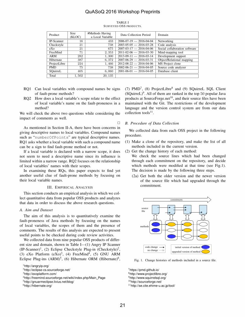
TABLE ISURVEYED OSS PRODUCTS.

Product Size(KLOC)

#Methods Havinga Local Variable

Data Collection Period Domain

IP-Scanner 16 433 2006-07-19 — 2016-04-04 NetworkingCheckstyle 21 738 2003-05-05 — 2016-03-28 Code analysiseXo 21 675 2007-03-17 — 2016-04-06 Social collaboration softwareFreeMind 71 2, 353 2011-02-06 — 2016-03-30 Mind-mapping toolARM 282 1, 300 2013-09-11 — 2016-03-14 Development supportHibernate 387 6, 372 2007-06-29 — 2016-03-31 Object/Relational mappingProjectLibre 224 1, 466 2012-08-22 — 2016-04-06 MS Project clonePMD 75 738 2002-06-21 — 2016-04-05 Source code analyzerSQuirreL 405 6, 060 2001-06-01 — 2016-04-05 Database clientTotal 1, 502 20, 135

RQ1 Can local variables with compound names be signsof fault-prone methods?

RQ2 How does a local variable’s scope relate to the effectof local variable’s name on the fault-proneness in amethod?

We will check the above two questions while considering theimpact of comments as well.

2

As mentioned in Section II-A, there have been concerns ingiving descriptive names to local variables. Compound namessuch as “numberOfPoints” are typical descriptive names.RQ1 asks whether a local variable with such a compound namecan be a sign to find fault-prone method or not.

If a local variable is declared with a narrow scope, it doesnot seem to need a descriptive name since its influence islimited within a narrow range. RQ2 focuses on the relationshipof local variables’ names with their scopes.

In examining these RQs, this paper expects to find yetanother useful clue of fault-prone methods by focusing ontheir local variable names.

III. EMPIRICAL ANALYSIS

This section conducts an empirical analysis in which we col-lect quantitative data from popular OSS products and analyzesthat data in order to discuss the above research questions.

A. Aim and Dataset

The aim of this analysis is to quantitatively examine thefault-proneness of Java methods by focusing on the namesof local variables, the scopes of them and the presence ofcomments. The results of this analysis are expected to presentuseful points to be checked during code review activities.

We collected data from nine popular OSS products of differ-ent size and domain, shown in Table I—(1) Angry IP Scanner(IP-Scanner)1, (2) Eclipse Checkstyle Plug-in (Checkstyle)2,(3) eXo Platform (eXo)3, (4) FreeMind4, (5) GNU ARMEclipse Plug-ins (ARM)5, (6) Hibernate ORM (Hibernate)6,

1http://angryip.org/2http://eclipse-cs.sourceforge.net/3http://exoplatform.com/4http://freemind.sourceforge.net/wiki/index.php/Main Page5http://gnuarmeclipse.livius.net/blog/6http://hibernate.org/

(7) PMD7, (8) ProjectLibre8 and (9) SQuirreL SQL Client(SQuirreL)9. All of them are ranked in the top 50 popular Javaproducts at SourceForge.net10, and their source files have beenmaintained with the Git. The restrictions of the developmentlanguage and the version control system are from our datacollection tools11.

B. Procedure of Data Collection

We collected data from each OSS project in the followingprocedure.

(1) Make a clone of the repository, and make the list of allmethods included in the current version.

(2) Get the change history of each method:We check the source lines which had been changedthrough each commitment on the repository, and decidewhich methods were modified at that time (see Fig.1).The decision is made by the following three steps.(2a) Get both the older version and the newer version

of the source file which had upgraded through thecommitment.

Fig. 1. Change histories of methods included in a source file.

7https://pmd.github.io/8http://www.projectlibre.org/9http://www.squirrelsql.org/10http://sourceforge.net/11http://se.cite.ehime-u.ac.jp/tool/


21

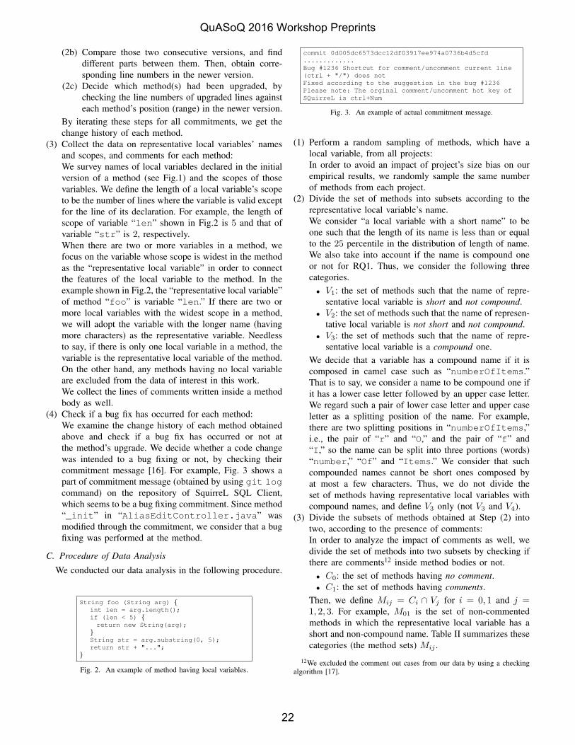
(2b) Compare those two consecutive versions, and finddifferent parts between them. Then, obtain corre-sponding line numbers in the newer version.

(2c) Decide which method(s) had been upgraded, bychecking the line numbers of upgraded lines againsteach method’s position (range) in the newer version.

By iterating these steps for all commitments, we get thechange history of each method.

(3) Collect the data on representative local variables’ namesand scopes, and comments for each method:We survey names of local variables declared in the initialversion of a method (see Fig.1) and the scopes of thosevariables. We define the length of a local variable’s scopeto be the number of lines where the variable is valid exceptfor the line of its declaration. For example, the length ofscope of variable “len” shown in Fig.2 is 5 and that ofvariable “str” is 2, respectively.When there are two or more variables in a method, wefocus on the variable whose scope is widest in the methodas the “representative local variable” in order to connectthe features of the local variable to the method. In theexample shown in Fig.2, the “representative local variable”of method “foo” is variable “len.” If there are two ormore local variables with the widest scope in a method,we will adopt the variable with the longer name (havingmore characters) as the representative variable. Needlessto say, if there is only one local variable in a method, thevariable is the representative local variable of the method.On the other hand, any methods having no local variableare excluded from the data of interest in this work.We collect the lines of comments written inside a methodbody as well.

(4) Check if a bug fix has occurred for each method:We examine the change history of each method obtainedabove and check if a bug fix has occurred or not atthe method’s upgrade. We decide whether a code changewas intended to a bug fixing or not, by checking theircommitment message [16]. For example, Fig. 3 shows apart of commitment message (obtained by using git logcommand) on the repository of SquirreL SQL Client,which seems to be a bug fixing commitment. Since method“_init” in “AliasEditController.java” wasmodified through the commitment, we consider that a bugfixing was performed at the method.

C. Procedure of Data Analysis

We conducted our data analysis in the following procedure.

String foo (String arg) {int len = arg.length();if (len < 5) {return new String(arg);

}String str = arg.substring(0, 5);return str + "...";

}

Fig. 2. An example of method having local variables.

commit 0d005dc6573dcc12df03917ee974a0736b4d5cfd.............Bug #1236 Shortcut for comment/uncomment current line(ctrl + "/") does notFixed according to the suggestion in the bug #1236Please note: The orginal comment/uncomment hot key ofSQuirreL is ctrl+Num

Fig. 3. An example of actual commitment message.

(1) Perform a random sampling of methods, which have alocal variable, from all projects:In order to avoid an impact of project’s size bias on ourempirical results, we randomly sample the same numberof methods from each project.

(2) Divide the set of methods into subsets according to therepresentative local variable’s name.We consider “a local variable with a short name” to beone such that the length of its name is less than or equalto the 25 percentile in the distribution of length of name.We also take into account if the name is compound oneor not for RQ1. Thus, we consider the following threecategories.

• V1: the set of methods such that the name of repre-sentative local variable is short and not compound.

• V2: the set of methods such that the name of represen-tative local variable is not short and not compound.

• V3: the set of methods such that the name of repre-sentative local variable is a compound one.

We decide that a variable has a compound name if it iscomposed in camel case such as “numberOfItems.”That is to say, we consider a name to be compound one ifit has a lower case letter followed by an upper case letter.We regard such a pair of lower case letter and upper caseletter as a splitting position of the name. For example,there are two splitting positions in “numberOfItems,”i.e., the pair of “r” and “O,” and the pair of “f” and“I,” so the name can be split into three portions (words)“number,” “Of” and “Items.” We consider that suchcompounded names cannot be short ones composed byat most a few characters. Thus, we do not divide theset of methods having representative local variables withcompound names, and define V3 only (not V3 and V4).

(3) Divide the subsets of methods obtained at Step (2) intotwo, according to the presence of comments:In order to analyze the impact of comments as well, wedivide the set of methods into two subsets by checking ifthere are comments12 inside method bodies or not.

• C0: the set of methods having no comment.• C1: the set of methods having comments.

Then, we define Mij = Ci ∩ Vj for i = 0, 1 and j =1, 2, 3. For example, M01 is the set of non-commentedmethods in which the representative local variable has ashort and non-compound name. Table II summarizes thesecategories (the method sets) Mij .

12We excluded the comment out cases from our data by using a checkingalgorithm [17].


22

TABLE IISYMBOLS REPRESENTING CATEGORIES.

Name of representative local variableSymbol Non-compound

Compoundshort not shortNon-commented methods M01 M02 M03

Commented methods M11 M12 M13

(4) Examine the fault-proneness of methods by the abovecategories Mij :We statistically compare the bug fix rates among cate-gories Mij (for i = 0, 1 and j = 1, 2, 3) and discuss theresults.

(5) Examine the trends of the bug fix rates over scope:In order to analyze the impact of variable’s scope as well,we analyze the changes in bug fix rate by varying therange (the length of scope) which we focus on. In theconcrete, we compare the moving averages of the bug fixrates among categories Mij (for i = 0, 1 and j = 1, 2, 3),by varying the range of focusing scope.

D. Results and Discussion: Collected Data

We first show the results of our data collection. Since theminimum number of methods included in a project was 433 asshown in Table I (project “IP-Scanner”), we randomly sampled400 methods from each project, so our dataset consists of3, 600 methods in total.

Table III shows the distributions of length of representativelocal variables’ names in character count and in word count,respectively. Here, “word count” means the number of wordscomposing a variable’s name which is split according to thenotion of the camel case. The longest names in character countwere “containsSuppressWarningsHolderModule”and “organizationInitializersHomePathNode”which consist of 36 characters, and the longest name inword count was “thereWereNodesToBeFolded” whichconsists of 6 words. Although such some long and descriptivenames appear in some methods, most local variables havenames that consist of at most a few characters and they arenon-compound names whose word count is one. Since the25 percentile (Q1) of the character count is four as shown inTable III, we will consider a name whose length is less thanor equal to four letters to be short in the following analysis.

Table IV presents the distribution of length of a represen-tative local variable’s scope. Since there were some methodsas shown in Fig.4, where the minimum length of the scope iszero. As all local variables are valid only within a (part of the)

TABLE IIIDISTRIBUTION OF LENGTH OF

REPRESENTATIVE LOCAL VARIABLE NAMES.

Unit Min. Q1 Median Q3 Max.Character 1 4 6 10 36

Word 1 1 1 2 6

(Q1: 25 percentile; Q3: 75 percentile)

TABLE IVDISTRIBUTION OF SCOPE OF REPRESENTATIVE LOCAL VARIABLES.

Min. Q1 Median Q3 Max.0 4 9 19 793


private void doConnectToRunningChanged() {if (doStartGdbServer.getSelection()) {boolean enabled = doConnectToRunning.getSelection();

}}

Fig. 4. An instance of local variable whose scope is zero (“enabled”).

method, the majority of them are around a few to ten lines ofcode. In order to filter out extreme data which may be noisein our analysis, we will use only the data whose scopes are inbetween 25 percentile (Q1 = 4) and 75 percentile (Q3 = 19)of their distribution. By this data filtering, the number of oursamples are reduced to 1, 872. Table V gives the number ofmethods belong to each category Mij (for i = 0, 1; j = 1, 2, 3)after this filtering.

Table VI shows the distribution of the number of bug fixeswhich had occurred in methods over their upgrades. About18% of methods seemed to have had a hidden fault and havefixed through their code changes. Since we already filteredout the methods such that the scope of the representativelocal variable was wide, most of the methods in our datasetwere small-sized and thus possibly more simple in structure.Hence, conventional size metrics and structural complexitymetrics would be ineffective for analyzing the fault-pronenessof methods in detail. It would be worth it to focus on a featureof methods other than the size and complexity. A local variablename might be yet another useful feature to be focused on.

E. Results and Discussion: Comparison of Bug Fix Rates byCategory

Table VII presents the bug fix rate in each category Mij

(for i = 0, 1; j = 1, 2, 3). There seem to be differences in the

TABLE VNUMBER OF METHODS BELONG TO EACH CATEGORY.

Non-Compound CompoundCategory ≤ 4 > 4 Name TotalNon-Commented 401 527 427 1, 355

(M01) (M02) (M03) (C0)Commented 139 164 214 517

(M11) (M12) (M13) (C1)Total 540 691 641 1, 872

(V1) (V2) (V3)

TABLE VIDISTRIBUTION OF NUMBER OF BUG FIXES

OBSERVED IN METHODS AND BUG FIX RATE.

Min. Q1 Median Q3 Max. Rate0 0 0 0 5 18.1%



23

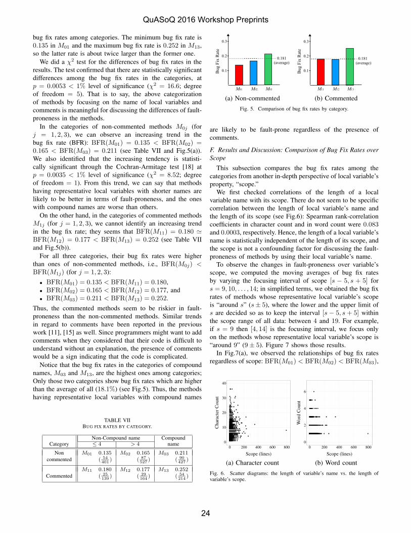
bug fix rates among categories. The minimum bug fix rate is0.135 in M01 and the maximum bug fix rate is 0.252 in M13,so the latter rate is about twice larger than the former one.

We did a χ2 test for the differences of bug fix rates in theresults. The test confirmed that there are statistically significantdifferences among the bug fix rates in the categories, atp = 0.0053 < 1% level of significance (χ2 = 16.6; degreeof freedom = 5). That is to say, the above categorizationof methods by focusing on the name of local variables andcomments is meaningful for discussing the differences of fault-proneness in the methods.

In the categories of non-commented methods M0j (forj = 1, 2, 3), we can observe an increasing trend in thebug fix rate (BFR): BFR(M01) = 0.135 < BFR(M02) =0.165 < BFR(M03) = 0.211 (see Table VII and Fig.5(a)).We also identified that the increasing tendency is statisti-cally significant through the Cochran-Armitage test [18] atp = 0.0035 < 1% level of significance (χ2 = 8.52; degreeof freedom = 1). From this trend, we can say that methodshaving representative local variables with shorter names arelikely to be better in terms of fault-proneness, and the oneswith compound names are worse than others.

On the other hand, in the categories of commented methodsM1j (for j = 1, 2, 3), we cannot identify an increasing trendin the bug fix rate; they seems that BFR(M11) = 0.180 ≃BFR(M12) = 0.177 < BFR(M13) = 0.252 (see Table VIIand Fig.5(b)).

For all three categories, their bug fix rates were higherthan ones of non-commented methods, i.e., BFR(M0j) <BFR(M1j) (for j = 1, 2, 3):

• BFR(M01) = 0.135 < BFR(M11) = 0.180,• BFR(M02) = 0.165 < BFR(M12) = 0.177, and• BFR(M03) = 0.211 < BFR(M13) = 0.252.

Thus, the commented methods seem to be riskier in fault-proneness than the non-commented methods. Similar trendsin regard to comments have been reported in the previouswork [11], [15] as well. Since programmers might want to addcomments when they considered that their code is difficult tounderstand without an explanation, the presence of commentswould be a sign indicating that the code is complicated.

Notice that the bug fix rates in the categories of compoundnames, M03 and M13, are the highest ones among categories;Only those two categories show bug fix rates which are higherthan the average of all (18.1%) (see Fig.5). Thus, the methodshaving representative local variables with compound names

TABLE VIIBUG FIX RATES BY CATEGORY.

Non-Compound name CompoundCategory ≤ 4 > 4 name

Non M01 0.135 M02 0.165 M03 0.211commented ( 54

401) ( 87

527) ( 90

427)

M11 0.180 M12 0.177 M13 0.252Commented ( 25

139) ( 29

164) ( 54

214)

(a) Non-commented (b) CommentedFig. 5. Comparison of bug fix rates by category.

are likely to be fault-prone regardless of the presence ofcomments.

F. Results and Discussion: Comparison of Bug Fix Rates overScope

This subsection compares the bug fix rates among thecategories from another in-depth perspective of local variable’sproperty, “scope.”

We first checked correlations of the length of a localvariable name with its scope. There do not seem to be specificcorrelation between the length of local variable’s name andthe length of its scope (see Fig.6): Spearman rank-correlationcoefficients in character count and in word count were 0.083and 0.0003, respectively. Hence, the length of a local variable’sname is statistically independent of the length of its scope, andthe scope is not a confounding factor for discussing the fault-proneness of methods by using their local variable’s name.

To observe the changes in fault-proneness over variable’sscope, we computed the moving averages of bug fix ratesby varying the focusing interval of scope [s − 5, s + 5] fors = 9, 10, . . . , 14; in simplified terms, we obtained the bug fixrates of methods whose representative local variable’s scopeis “around s” (s± 5), where the lower and the upper limit ofs are decided so as to keep the interval [s − 5, s + 5] withinthe scope range of all data: between 4 and 19. For example,if s = 9 then [4, 14] is the focusing interval, we focus onlyon the methods whose representative local variable’s scope is“around 9” (9± 5). Figure 7 shows those results.

In Fig.7(a), we observed the relationships of bug fix ratesregardless of scope: BFR(M01) < BFR(M02) < BFR(M03),

0

10

20

30

40

0 200 400 600 800

Scope (lines)

Char

acte

r C

ount

0

2

4

6

0 200 400 600 800

Scope (lines)

Word

Count

(a) Character count (b) Word countFig. 6. Scatter diagrams: the length of variable’s name vs. the length ofvariable’s scope.


24

which are similar to the results shown in Fig.5(a). Thus, wecan say with emphasis: while the fault-proneness of methodshaving representative local variables with shorter names arelow, the methods having representative local variables withcompound names are high. Since the gap in the bug fix ratebetween M01 and M02 becomes smaller as the scope getswider, the superiority of a shorter name may be limited to anarrower scope. If a local variable with a short and simplename is used in a wider scope, it might cause an abuse of thevariable or a poor understandability of the program’s behavior.While Kernighan and Pike [10] said to give a short and simplename to a local variable, they did not recommend such anaming in any case, and their argument supposed the casethat a local variables was used in just “locally” within a partof a program. The results observed in Fig.7(a) seem to supportsuch a programming heuristic.

In Fig.7(b), while M11 (≤ 4 letters) are better than M12

(> 4 letters) with narrower scopes around 9 or 10, theirmagnitude relationship inverts as their scope gets wider. Thatwould be the reason why BFR(M11) ≃ BFR(M12) inFig.5(b). Therefore, we can say that a shorter name is betterwith a narrower scope, but cannot claim a shorter name isalways better. If programmers wanted to add comments, therewould be a lack of clarity in their code. In such a case, ashorter name with a wider scope might spur the program’spoor comprehensibility. On the other hand, compound namesalways show the worst (highest) bug fix rates regardless ofscope, similar to the results in Fig.7(a). Although compoundnames are usually descriptive, they seem to be signs of fault-prone methods. If a programmer wanted to give a compoundname to a local variable, the role of the variable would besomewhat complicated, so methods having such local variablesmight be riskier than the others in terms of fault-proneness.

G. Answers to RQs

From the results of Sections III-E and III-F, we summarizeour findings for RQ1 and RQ2 in the following.

For RQ1, we conclude that methods having local variableswith compound names are likely to be faulty regardless ofscope. Although we do not imply that compound names cause

0.0

0.1

0.2

10 12 14

Central Scope

Bug F

ix R

ate

0.0

0.1

0.2

10 12 14

Central Scope

Bug F

ix R

ate

(a) Non-commented (b) Commented

Fig. 7. Moving averages of bug fix rates over scope.

faults in methods, the presence of a local variable with acompound name may be a clue finding a risky part from theperspective of the fault-proneness in a method. Such a localvariable might have an important role or a more complex rolein the program, so they have to be reviewed more carefully.

For RQ2, we can say that shorter names are better for localvariables with narrower scope. As a scope gets wider, the posi-tive effect of shorter names seems to be decayed. While a shortand simple name would be preferable as mentioned in somecoding conventions and programmers’ heuristics [8], [9], [10],our empirical results quantitatively showed that the variable’sscope is also a feature worthy of consideration. Moreover, thepresence of comments may degrade the superiority of shorternames as their scopes get wider. Therefore, we should take intoaccount not only the composition of local variable’s name butalso its scope and comments in the code review.

H. Threats to Validity

This empirical analysis has been conducted for Java prod-ucts. While another programming language might producedifferent results, there would not be essential differences inthe concept of local variables and comments, among Javaand many other modern programming languages. Thus, thedifference in programming language would not be a seriousthreat to validity.

In order to avoid the data selection bias, we adopted arandom sampling in our data collection. Moreover, we usedpopular different sized OSS products from different domains.Therefore, our construction of dataset would not be a threatto validity.

Since our data is collected from the initial version ofthe methods, some methods might be no longer used today.However, all methods in our dataset are included in the latestversion of the product because we made our method list bychecking the latest version of their source files as describedin Section III-B. Moreover, we did a random sampling fromthem. Thus, we consider it will not be a serious threat tovalidity in our empirical work.

Our definition of compound name is based on the notionof camel case. If there are local variables whose namesare composed by another rule such as the snake case, e.g.,“number_of_items,” they are wrongly categorized intonon-compound names. Thus, we rechecked all representa-tive local variables’ names included in our data set, thenwe found only two variables having snake case names,“s_descriptors” and “size_h.” Due to the small num-ber of error cases, our name splitting method was not a seriousthreat to validity.

IV. RELATED WORK

Lawrie et al. conducted a survey on names of identifiers interms of their comprehensibility for over 100 programmers [7].In their survey research, they classified names of identifiersinto three categories (1) fully-spelled name, (2) abbreviatedname and (3) initial letter—for example, (1) “count,” (2)“cnt” and (3) “c”—, then compared their understandability.


25

Their results showed that fully-spelled names were the easiestto understand but that there did not seem to be significantdifferences with abbreviated names in their comprehensibilitylevel. While their work provides a useful motivation to studywhether a shorter name is better or not, they did not discussthe fault-proneness of program.

Kawamoto and Mizuno [19] conducted an empirical studywith two OSS products and reported that a class includinga long identifier tends to be faulty. While their work is oneof our most significant previous studies, our work focuseson a finer-grained artifact—local variable—and conducts astatistical analysis with taking into account of the scopes andthe comments.

Binkley et al. [20] focused on the relationship be-tween the length of identifier (including a variable’s name,a method’s name and a class’s name) and the humanshort-term memory. They identified that identifiers withlong names are related to a difficulty in program com-prehension. They were concerned that a long chain, e.g.,“class.firstAssignment().name.trim(),” wouldcause a loss of the readability of the code. While the researchviewpoint differs from our work, the fundamental concernabout the length of name is common, and it seems to be wellaccorded with our results showing the compound names arenot recommended for local variables.

Aman et al. [11] reported an empirical analysis showingthat Java methods having local variables with long names aremore likely to be fault-prone and change-prone than the othermethods. That report is our significant previous work, and thispaper focuses more detailed features of local variables, i.e., thecomposition of name and their scopes. While another work byAman et al. [15], reporting that commented programs tend tobe more fault-prone, is also our important previous work, weconduct a further analysis examining combinations of the localvariable’s name, the scope and the comments in this paper.

V. CONCLUSION

We have focused on programming artifacts which mayvary among individuals: local variables’ names and comments.Popular code conventions say that names of local variablesshould be shorter and simple, and it seems to have beena heuristic of programmers. We empirically evaluated theheuristic in terms of fault-proneness by checking the namesof local variables, their scopes and the presence of comments.The empirical analysis for the data from nine popular OSSproducts showed the following three findings.(1) Local variables with compound names can be signs of

fault-prone methods.(2) Methods having the representative local variables with

non-compound and shorter names (≤ 4 letters) are lessfault-prone, but their positive effects are decayed as theirscopes get wider (around 10 or more lines).

(3) Methods having comments in their bodies are also morelikely to be faulty.

These findings are expected to be useful guidelines for moreefficient code reviews.

One of our significant future works is to conduct furtheranalyses of local variables’ names, which include an ap-plication of the natural language processing technologies toevaluate the meaning of local variables’ names. A furtheranalysis with products written in a programming languageother than Java is also our future project in order to ensurethe generality of the above findings.

ACKNOWLEDGMENT

This work was supported by JSPS KAKENHI #16K00099.The authors would like to thank anonymous reviewers for theirhelpful comments.

REFERENCES

[1] G. J. Myers, C. Sandler, and T. Badgett, The Art of Software Testing.N.J.: John Wiley & Sons, 2004.

[2] P. C. Rigby and C. Bird, “Convergent contemporary software peerreview practices,” in Proc. 9th Joint Meeting on Foundations of Softw.Eng., Aug. 2013, pp. 202–212.

[3] P. L. Li, J. Herbsleb, M. Shaw, and B. Robinson, “Experiencesand results from initiating field defect prediction and product testprioritization efforts at ABB Inc.” in Proc. 28th Int’l Conf. Softw. Eng.,May 2006, pp. 413–422.

[4] S. Lessmann, B. Baesens, C. Mues, and S. Pietsch, “Benchmarking clas-sification models for software defect prediction: A proposed frameworkand novel findings,” IEEE Trans. Softw. Eng., vol. 34, no. 4, pp. 485–496, July 2008.

[5] Y. Liu, T. Khoshgoftaar, and N. Seliya, “Evolutionary optimizationof software quality modeling with multiple repositories,” IEEE Trans.Softw. Eng., vol. 36, no. 6, pp. 852–864, Nov 2010.

[6] F. Rahman and P. Devanbu, “How, and why, process metrics are better,”in Proc. 2013 Int’l Conf. Softw. Eng., May 2013, pp. 432–441.

[7] D. Lawrie, C. Morrell, H. Feild, and D. Binkley, “What’s in a name? astudy of identifiers,” in Proc. 14th Int’l Conf. Program Comprehension,June 2006, pp. 3–12.

[8] Free Software Foundation, “Gnu coding standards,”https://www.gnu.org/prep/standards/.

[9] Sun Microsystems, “Code conventions for the java program-ming language,” http://www.oracle.com/technetwork/java/codeconvtoc-136057.html.

[10] B. W. Kernighan and R. Pike, The practice of programming. Boston,MA: Addison-Wesley Longman, 1999.

[11] H. Aman, S. Amasaki, T. Sasaki, and M. Kawahara, “Empirical analysisof change-proneness in methods having local variables with long namesand comments,” in Proc. 2015 ACM/IEEE Int’l Symp. Empirical Softw.Eng. and Measurement, Oct. 2015, pp. 50–53.

[12] M. J. Sousa and H. Moreira, “A survey on the software maintenanceprocess,” in Proc. Int’l Conf. Softw. Maintenance, Nov. 1998, pp. 265–274.

[13] R. P. Buse and W. R. Weimer, “A metric for software readability,” inProc. 2008 Int’l Symp. Softw. Testing and Analysis, 2008, pp. 121–130.

[14] M. Fowler, Refactoring: Improving the Design of Existing Code.Boston, MA: Addison-Wesley Longman, 1999.

[15] H. Aman, S. Amasaki, T. Sasaki, and M. Kawahara, “Lines of commentsas a noteworthy metric for analyzing fault-proneness in methods,” IEICETrans. Inf. & Syst., vol. E98-D, no. 12, pp. 2218–2228, Dec. 2015.

[16] J. Sliwerski, T. Zimmermann, and A. Zeller, “When do changes inducefixes?” in Proc. Int’l Workshop on Mining Softw, Repositories, May2005, pp. 1–5.

[17] H. Aman, “An empirical analysis of the impact of comment statementson fault-proneness of small-size module,” in Proc. 19th Asia-PacificSoftw. Eng. Conf., Dec. 2012, pp. 362–367.

[18] A. Agresti, Categorical Data Analysis, 2nd ed. N.J.: Wiley, 2002.[19] K. Kawamoto and O. Mizuno, “Predicting fault-prone modules using the

length of identifiers,” in Proc. 4th Int’l Workshop on Empirical Softw.Eng. in Practice, Oct. 2012, pp. 30–34, Japan.

[20] D. Binkley, D. Lawrie, S. Maex, and C. Morrell, “Identifier lengthand limited programmer memory,” Science of Computer Programming,vol. 74, no. 7, pp. 430–445, May 2009.


26

Towards improved Adoption: Effectiveness ofResearch Tools in the Real World

Richa AwasthyAustralian National University

Canberra, AustraliaEmail: [email protected]

Shayne FlintResearch School of Computer Science

Australian National UniversityCanberra, Australia

[email protected]

Ramesh SankaranarayanaResearch School of Computer Science

Australian National UniversityCanberra, Australia

[email protected]

Abstract—One of the challenges in the area of software engi-neering research has been the low rate of adoption by industryof the tools and methods produced by university researchers. Wepresent a model to improve the situation by providing tangibleevidence that demonstrates the real-world effectiveness of suchtools and methods. A survey of practising software engineersindicates that the approach in the model is valid and applicable.We apply and test the model for providing such evidence anddemonstrate its effectiveness in the context of static analysis usingFindBugs. This model can be used to analyse the effectivenessof academic research contributions to industry and contributetowards improving their adoption.

I. INTRODUCTION

The success of software engineering research in universi-ties can be measured in terms of the industrial adoption ofmethods and tools developed by researchers. Current adoptionrates are low [1] and this contributes to a widening gapbetween software engineering research and practice. Consider,for example, code inspections, which according to Fagan’slaw, are effective in reducing errors in software, increasingproductivity and achieving project stability [2]. Static analysistools developed by university researchers help automate thecode inspection process. However, the use of such tools hasnot obtained widespread adoption in industry. One reason forthis limited adoption is that researchers often fail to providereal-world evidence that the methods and tools they developare of potential value to industry practitioners [1], [3].

One approach to providing such evidence is to conductexperiments that demonstrate the effectiveness of researchtools in a real-world context. We apply this approach toanalyse the effectiveness of a static analysis tool. In doingso, we demonstrate that such experimentation can contributeto closing the gap between research and practice.

The structure of this paper is as follows: Section II providesthe background of our work leading to the proposed model;Section III presents a survey which shows that real worldevidence can positively influence the decision of softwareengineers to use research tools; Section IV explains ourexperimental method which uses FindBugs [4] to analyse realworld bugs in Eclipse [5] code; Section V discusses howsimple experiments like ours can encourage more developersto use tools developed by researchers and thus contribute toclosing the gap between research and practice. Section VI

provides an overview of related research; Section VII presentsconclusions and discusses future research.

II. BACKGROUND

Since the 1970’s there have been ongoing efforts to increasethe adoption of research outcomes outside of universities [6].As a result of the United States Bayh Dole Act in 1980[7], universities began to establish Technology Transfer Offices(TTOs) to facilitate the transfer of knowledge from universitiesto industry [8]. However, the effectiveness of TTOs has beenquestioned in recent years [9], [10] and there is a need tolook beyond TTOs to improve adoption of academic researchin industry.

Researchers in universities are working towards addressingsignificant problems. The outcome of their work can be atool or method which may or may not achieve wide-spreadindustry adoption. A key factor limiting the readiness of theseresearch outcomes for adoption in industry is a lack of tangibleevidence that they would be effective in practice [1]. Thissuggests that demonstrating the effectiveness of a tool inpractice can contribute to improved adoption.

Figure 1 depicts our model for demonstrating the real-world effectiveness of research tools and methods. The modelinvolves 4 steps with intermediate activities. First step isto identify a problem to address. Step 2 is to develop atool or a method to address the problem. The intermediateiterative activity involved between these 2 steps is the processof solution formulation, which involves adding new ideas tothe available state of the art. These steps are followed byiterative testing for validation in Step 3. Step 3 confirmsthe readiness of the research outcome for adoption. An ideashould be validated in a practical setting [11] to improve itsadoption. Our model respects this viewpoint and emphasisesthe importance of tangible evidence from a practical settingin Step 4. Researchers should test their research outcomesin a scenario that involves real world users who are animportant stakeholder for industry to increase the relevance ofthe evidence for industry. Demonstrating the effectiveness ofresearch outcomes in real-world scenario will lead to changein industry perception and improved adoption of the researchoutcomes.


27

We test the applicability of this model in the static analysiscontext by identifying a static analysis tool created by univer-sity researchers and analysing its effectiveness in a real-worldscenario.

Problem Develop a

Tool/method Test in the

lab

Test in the real

environment

Improved Industrial Adoption

of the tool

Solution Formulation

Ready for testing

Effectiveness leading to

University Research

Modify

Ready for adoption

1 2 3

4

Fig. 1. Proposed model for improving adoption of university research byindustry

III. THE IMPACT OF EVIDENCE FROM REAL-WORLDSCENARIO

In order to understand the impact of evidence from a user-scenario on real-world decisions to use a research tool, weconducted an on-line survey of software developers.

The survey uses static analysis as an example and wasprepared and delivered using our university’s online pollingsystem [12]. Participants were invited by email which includeda link to the on-line survey and a participant informationstatement. On completion of the survey, we manually analysedthe results.

III.B.1

III.B.2

III.B.3

Fig. 2. Flowchart for the survey questionnaire design

A. Participants

We invited 20 software industry practitioners and around10 computer science researchers with industry experience insoftware development.

B. Survey Questions

The survey data consisted of responses to the sequence ofquestions depicted in Figure 2 and described below.

1) Software engineering experience: We gathered informa-tion about the level of software development expertise of eachparticipant so that we can understand any relationship betweenexperience and use of static analysis tools.

2) Static analysis knowledge: We asked the following ques-tions to determine each participant’s level of understanding anduse of static analysis tools.

a) ‘Static analysis is the analysis of computer softwareto find potential bugs without actually executing thesoftware. Have you heard of static analysis before?’

b) ‘Have you used any automated static analysis toolsduring software development (e.g. FindBugs, Coverity)?’

Answers to these questions were used to determine the finalquestion we asked, as indicated in Figure 2.

3) The impact of the tangible evidence: At the end of thesurvey each participant who has not used static analysis toolswas asked a question to determine the impact that tangibleevidence (that the tool can identify real bugs early in thesoftware development life-cycle) might have on their approachto static analysis. The exact question asked depended on theiranswers to questions described in Section III-B2. Specifically:

1) Participants who had no knowledge of static analysis wereasked ‘Would our research results interest you in gainingknowledge of static analysis and adoption of automatedstatic analysis tools?’.

2) Participants who knew about static analysis but had notused any static analysis tools (our primary group ofinterest) were asked to rate the impact that the followingfactors would have on their decision to adopt staticanalysis tools. A Likert scale was used with 5 options (Noinfluence, May be, Likely, Highly Likely, and Definitely).

a) Effectiveness of tool in finding bugsb) Ease of usec) Integration of tool to development environment.d) License type.e) The availability of tangible evidence that the tool can

identify real bugs early in the software developmentlife-cycle - before they are reported by users.

C. Analysis of Survey Results

The response rate for our survey was high with 27 responsesout of 30 invitations. Responses to the survey indicate thattangible evidence of real-world effectiveness of a tool haspositive impact on decisions to adopt static analysis tools.

Analysis of the survey results provides the following spe-cific findings:


28

1) Software Engineering Experience - As expected, partici-pants had varied level of experience in software devel-opment. However, we do not find any direct relationbetween the experience and usage of tools.

2) Static Analysis Knowledge - Survey results show that9 participants (33%) had no prior knowledge of staticanalysis. It is noteworthy that while the remaining 18participants knew about static analysis, only 4 of themhad used static analysis tools.

3) Impact of the tangible evidence - Our survey results showthat tangible evidence has a positive impact on decisionsto adopt static analysis tools. Out of the 9 respondentswho had no prior knowledge of static analysis, 8 said thattangible evidence would interest them in gaining knowl-edge of static analysis and adopting automated staticanalysis tools. This is a valuable information indicatingthat providing evidence of effectiveness could contributeto improved adoption of research tools in industry.Of the 14 participants who had knowledge of staticanalysis but who had not used any tools, 7 participants(50%) indicated that tangible evidence would be HighlyLikely or would Definitely influence their decision toadopt static analysis tools (Figure 3). Another four par-ticipants indicated that such evidence would be Likelyto influence their decision. Considering the response ofthree participants as May be, it is possible that theyrespond positively, which will add to the percentage ofparticipants agreeing that tangible evidence will influencethe decision.

None May be Likely Highly likely Definitely0

0.5

1

1.5

2

2.5

3

3.5

4

4.5

Positive influence on decisions to adopt static analysis tool

Nu

mb

er

of P

art

icip

an

ts

Fig. 3. The impact of tangible evidence on decisions to adopt static analysistools

As shown in Figure 4, our results also indicate that otherfactors such as Ease of use, IDE integration and Licensetype have a positive impact on decisions to adopt staticanalysis tools. It is interesting to note that under the Maybe and Definitely category, the top two influencing factorsare License and Tangible evidence.

Our results clearly show that tangible evidence is an impor-tant factor in influencing decisions to adopt research tools inindustry.

None May be Likely Highly likely Definitely0

1

2

3

4

5

6

7

Effectiveness of tool

Ease of use

Integration to IDE

License

Tangible evidence

Influence of the factor

Nu

mb

er

of p

art

icip

an

ts

Fig. 4. Other factors influencing decisions to adopt static analysis tools

IV. APPLICABILITY OF THE MODEL

In order to test the applicability of our proposed model,we first had to identify an appropriate tool developed byresearchers and a scenario to test its effectiveness. FindBugsversion 3.0 was chosen for our research as according to thetool’s website, there are few organizations using FindBugs[4]. This indicates low adoption of the tool in softwareindustry. Also, it is an open-source static analysis tool witha university’s trademark. We conducted an experiment withthe FindBugs static analysis tool to analyse its effectivenessin the real world. To analyse the effectiveness in real-world,we wanted to determine if FindBugs is capable of findingbugs reported by real users of Eclipse. To do so, we adoptedan approach to establishing a connection between warningsgenerated by the FindBugs static analysis tool and field bugsreported by Eclipse users on Bugzilla [13] that includes thebelow steps:

1) Use FindBugs to identify potential bugs in Eclipse classfiles.

2) Search the Eclipse bug-tracking system Bugzilla to iden-tify bug reports that include stack traces.

3) Match the code pointed in Java classes associated withFindBugs warnings identified in 1) with code pointed bystack trace associated with the bugs identified in 2).

A. FindBugs

FindBugs analyses Java class files to report warnings andpotential errors in the associated source code. The tool per-forms analysis on Java class files without needing access tothe source code. It is stable, easy to use, and as mentionedin [14] has higher precision compared to other tools such asCodePro Analytix, PMD and UCDetector. It has a low rateof false positives [15], and has more than 400 types of bugclassification along with categorization based on severity level.The analysis is based on bug patterns which are classifiedinto nine categories: Bad Practice, Correctness, Experimen-tal, Internationalization, Malicious Code Vulnerability, Multi-threaded Correctness, Performance, Security, and Dodgy Code.The warnings reported by FindBugs can be further categorisedwithin the tool as: Scariest (Ranks 1-4), Scary (Ranks 1-9) andTroubling (Ranks 1-14). The category includes all the bugs


29

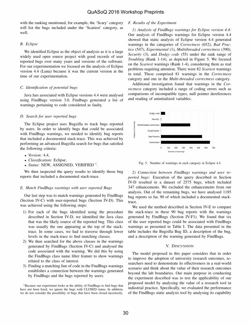
with the ranking mentioned, for example, the ‘Scary’ categorywill list the bugs included under the ‘Scariest’ category, aswell.

B. Eclipse

We identified Eclipse as the object of analysis as it is a largewidely used open source project with good records of userreported bugs over many years and versions of the software.For our experimentation we focused on the analysis of Eclipseversion 4.4 (Luna) because it was the current version at thetime of our experimentation.

C. Identification of potential bugs

Java Jars associated with Eclipse versions 4.4 were analysedusing FindBugs version 3.0. Findbugs generated a list ofwarnings pertaining to code considered as faulty.

D. Search for user reported bugs

The Eclipse project uses Bugzilla to track bugs reportedby users. In order to identify bugs that could be associatedwith FindBugs warnings, we needed to identify bug reportsthat included a documented stack-trace. This was achieved byperforming an advanced Bugzilla search for bugs that satisfiedthe following criteria:

• Version: 4.4,• Classification: Eclipse,• Status: NEW, ASSIGNED, VERIFIED 1.

We then inspected the query results to identify those bugreports that included a documented stack-trace.

E. Match FindBugs warnings with user reported Bugs

Our last step was to match warnings generated by FindBugs(Section IV-C) with user-reported bugs (Section IV-D). Thiswas achieved using the following steps:

1) For each of the bugs identified using the proceduredescribed in Section IV-D, we identified the Java classthat was the likely source of the reported bug. This classwas usually the one appearing at the top of the stack-trace. In some cases, we had to traverse through lowerlevels in the stack-trace to find matching classes.

2) We then searched for the above classes in the warningsgenerated by FindBugs (Section IV-C) and analysed thecode associated with the warning. We did this by usingthe FindBugs class name filter feature to show warningsrelated to the class of interest.

3) Finding a matching line of code in the FindBugs warningsestablishes a connection between the warnings generatedby FindBugs and the bugs reported by users.

1Because our experiment looks at the ability of FindBugs to find bugs thathave not been fixed, we ignore the bugs with CLOSED status. In addition,we do not consider the possibility of bugs that have been closed incorrectly.

F. Results of the Experiment

1) Analysis of FindBugs warnings for Eclipse version 4.4:Our analysis of FindBugs warnings for Eclipse version 4.4showed that static analysis of Eclipse version 4.4 generatedwarnings in the categories of Correctness (652), Bad Prac-tice (547), Experimental (1), Multithreaded correctness (390),Security (3), and Dodgy code (55) under the rank range ofTroubling (Rank 1-14), as depicted in Figure 5. We focusedon the Scariest warnings (Rank 1-4), considering them as realproblems requiring attention. There were 82 Scariest warningsin total. These comprised 81 warnings in the Correctnesscategory and one in the Multi-threaded correctness category.

Additional investigation found that warnings in the Cor-rectness category included a range of coding errors such ascomparisons of incompatible types, null pointer dereferencesand reading of uninitialized variables.

Correctness

Bad Practice

Experimental

Multithreaded correctness

Security

Dodgy code

0 100 200 300 400 500 600 700

Number of warnings

Ca

teg

ory

of w

arn

ing

s

Fig. 5. Number of warnings in each category in Eclipse 4.4

2) Connection between FindBugs warnings and user re-ported bugs: Execution of the query described in SectionIV-D resulted in a dataset of 2575 bugs, which included347 enhancements. We excluded the enhancements from ouranalysis. Out of the remaining bugs, we have analysed 1185bug reports so far, 90 of which included a documented stack-trace.

We used the method described in Section IV-E to comparethe stack-trace in these 90 bug reports with the warningsgenerated by FindBugs (Section IV-F1). We found that sixof the user reported bugs could be associated with FindBugswarnings as presented in Table I. The data presented in thetable includes the Bugzilla Bug ID, a description of the bug,and a description of the warning generated by FindBugs.

V. DISCUSSION

The model proposed in this paper considers that in orderto improve the adoption of university research outcomes, re-searchers need to demonstrate its effectiveness in a real-worldscenario and think about the value of their research outcomesbeyond the lab boundaries. Our main purpose in conductingthe experiment described was to test the applicability of ourproposed model by analysing the value of a research tool inindustrial practice. Specifically, we evaluated the performanceof the FindBugs static analysis tool by analysing its capability


30

TABLE IUSER-FILED BUGS IN ECLIPSE WITH ASSOCIATED WARNING IN FINDBUGS

Bug Id Problem Description FindBugs Warning436138 NPE when select SWT.MOZILLA style in

control exampleMethod call passes null for nonnull parameterThis method call passes a null value for anonnull method parameter. Either the parameter is annotated as a parameter that shouldalways be nonnull, or analysis has shown that it will always be dereferenced. Bug kindand pattern: NP - NP NULL PARAM DEREF

414508 NPE trying to launch Eclipse App Load of known null value. The variable referenced at this point is known to be null dueto an earlier check against null. Although this is valid, it might be a mistake (perhapsyou intended to refer to a different variable, or perhaps the earlier check to see if thevariable is null should have been a check to see if it was nonnull). Bug kind and pattern:NP - NP LOAD OF KNOWN NULL VALUE

433526 browser.getText() is throwing exception af-ter Internet Explorer 11 install

Possible null pointer dereference There is a branch of statement that, if executed, guaran-tees that a null value will be dereferenced, which would generate a NullPointerExceptionwhen the code is executed. Of course, the problem might be that the branch or statementis infeasible and that the null pointer exception can’t ever be executed; deciding that isbeyond the ability of FindBugs.Bug kind and pattern: NP - NP NULL ON SOME PATH

459025 Can’t right-click items in manifest editor’sextensions tab on OSX

Non-virtual method call passes null for nonnull parameter A possibly-null value ispassed to a nonnull method parameter. Either the parameter is annotated as a parameterthat should always be nonnull, or analysis has shown that it will always be dereferenced.Bug kind and pattern: NP - NP NULL PARAM DEREF NONVIRTUAL

427421 NumberFormatException in periodicWorkspace Save Job

Boxing/unboxing to parse a primitive A boxed primitive is created from a String, just toextract the unboxed primitive value. It is more efficient to just call the static parseXXXmethod.Bug kind and pattern: Bx - DM BOXED PRIMITIVE FOR PARSING

428890 Search view only shows default page (NPEin PageBookView.showPageRec)


426485 [EditorMgmt][Split editor] Each split causeseditors to be leaked


in generating warnings relating to real-world bugs reported byusers of the Eclipse IDE.

Our results indicate that FindBugs is capable of identifyingbugs that will manifest themselves as bugs reported by users.Since real-world evidence would influence the decision toadopt a tool as indicated in the survey results, FindBugsneeds to improve the percentage of such warnings to makethe evidence convincing. Currently, FindBugs does not havethe intelligence to track the bug among the list of false pos-itives that can manifest. Our research provides improvementdirections to FindBugs in identifying the important bugs fromthe warning base by analysing the historical data and user re-quirement. FindBugs results can be improved by introducing anew ‘user-impact’ category to classify the warnings which willpotentially have an impact in the client environment and hence,need immediate attention. For this, sufficient information fromindustrial practice needs to be applied into testing the researchtool.

The model appears simple but it is challenging for re-searchers to identify a scenario and approach users and/or datato demonstrate the effectiveness of their tool or methods. Itmight be difficult for them to find the user-filed data always.Also, once they have the data to demonstrate the effectiveness,they need a mechanism to propagate it to industry. Also,the concern about the relevance of research suggests that re-

searchers need to think about the relevance of the problem theyare trying to address. These factors indicate that universitiesand industry need to start collaborating at an early stage andconsider co-developing whenever possible and feasible. Thiscan pave a good start towards improving the relevance andadoption of research outcomes in general, and bridging thegap between industry and academia.

A. Limitations and Threats to Validity

Our experiments were limited by the small number ofEclipse bugs reported with a documented stack-trace. It isimportant to note that the ability to analyse only 90 of the1185 bugs considered reflects a limitation of our approachand does not reflect a limitation of FindBugs. There are somelimitations to the validity of our experiments:

1) FindBugs does not always point to the exact line numberreferred to in the stack trace. It might be possible thatthe source of error could be different from the warningsprovided by FindBugs.

2) While it is likely that the FindBugs warnings listed inTable I are the actual cause of the listed real-world bugsreported by Eclipse users, we cannot be certain of this.

3) As there is lack of literature detailing the use of staticanalysis tools like FindBugs by the Eclipse developmentteam, a comparison study was not feasible.


31

4) This test highlights the relevance of static analysis tools,though the effectiveness in real-world projects, particu-larly large scale projects, cannot be confirmed as the sam-ple size of our survey is small. However, by consideringthe sample sizes of 20 and 18 used in related studies [16],[17], we decided to proceed with our sample size of 27participants.

5) The conclusion might not be generalised as the resultsare specific to the static analysis context. The proposedmodel needs to be validated regarding the tools in otherphases of software development.

VI. RELATED WORK

Adoption of software engineering research outcomes inindustry practice has been a concern [1], [18]. There have beenongoing efforts to improve the adoption of research outcomessince the 1970’s. However, the efforts mainly focused onapproaches to increase university-industry collaboration forimproving adoption through technology transfer. These effortsinclude policy changes leading to establishment of TTOs inuniversities and proposing models for effective technologytransfer [8], [19]. However, TTOs generally focus on buildingcollaborative relationships between researchers and industry[20] rather than the readiness of research outcomes for adop-tion in industry. In this paper we demonstrated how somesimple experiments can analyse the effectiveness of softwareengineering research tools in practice. Specifically we analysedthe effectiveness of a static analysis tool.

Various experiments have been conducted to demonstratethe effectiveness of the FindBugs static analysis tool by show-ing that it is able to detect the specific problems it has beendesigned to detect [15], [21], [22]. However, our experimenthas been conducted in unconstrained environment that involvesreal-world scenario that has impacted clients. Ruthruff et al.[23] involved developers in determining which reports wereuseful and which ones were not. This information was usedto filter FindBugs warnings so that only those that developersfound useful were reported. We retrace the user-filed bug tothe warning generated by the static analysis tool. This canpave way to create an intelligent mechanism to prioritise bugsbased on user-impact.

Al Bessey et al. [24] identify several factors that impactedthe industry adoption of their static analysis tool Coverity [25].They include trust between the researchers and industry users,the number of false positives, and the capability of the toolto provide warnings relating to problems which have had asignificant impact on its users. Our work also confirms thattool’s capability is important. It also identifies that licensing,IDE integration and ease of use are significant factors.

Johnson et al. [16] investigated the reasons behind thelow adoption rate of static-analysis tools despite their provenbenefits in finding bugs. Their investigations confirmed thatlarge numbers of false positives is a major factor in lowadoption rates. We note that their findings were based on thesurvey of developers who had all used static analysis tools.This meant that authors were not able to comment on whether

low-adoption rates were due to a lack of awareness of staticanalysis tools among developers.

None of the work described above analyses the effectivenessof FindBugs in identifying problems that manifest themselvesas real-world bugs reported by users. The experiments de-scribed in this paper analyse the connection between warningsgenerated by the FindBugs static analysis tool and field defectsreported by Eclipse users on Bugzilla bringing in client intothe perspective. The experiments test the applicability of ourproposed model in the static analysis context.

VII. CONCLUSION AND FUTURE WORK

We have proposed a model to contribute towards improvingthe adoption of research tools by industry by demonstratingthe effectiveness of the tool in real world scenario. We havepresented a mechanism which involves a research tool as amedium of building tangible evidence. A survey of softwaredevelopers supports our hypothesis that such tangible evidenceof effectiveness of a tool can have a positive influence on real-world decisions to adopt static analysis tools.

Further experiment for testing the applicability of the modelin the static analysis context was conducted. In this experi-ment, by establishing a connection between user-reported bugsand warnings generated by the FindBugs static analysis tool,we have demonstrated the ability of static analysis tools toeliminate some defects before software is deployed. However,the evidence needs to be stronger regarding the number of suchconnections in order to be more convincing and improving theindustrial adoption of the tool.

Future research would present more detailed analysis ofthe complete list of the bugs found in Section IV-F2, whichwill provide us precise data about the effectiveness of thetool according to our approach. Our approach also presentsa scenario where industry and university researchers can worktogether to create more useful tools. We plan to discuss theseresults with the FindBugs development team to explore thepossibility of strengthening the evidence and devising a newclassification user-impact to indicate the warnings that wouldmanifest in client-environment.

Finally, we would like to adapt this approach to explore theeffectiveness of research tools involved in other phases of thesoftware development life-cycle.

REFERENCES

[1] D. Rombach and F. Seelisch, “Balancing agility and formalism insoftware engineering,” B. Meyer, J. R. Nawrocki, and B. Walter, Eds.Berlin, Heidelberg: Springer-Verlag, 2008, ch. Formalisms in SoftwareEngineering: Myths Versus Empirical Facts, pp. 13–25.

[2] A. Endres and H. D. Rombach, A handbook of software and systemsengineering: empirical observations, laws and theories. PearsonEducation, 2003.

[3] M. Ivarsson and T. Gorschek, “A method for evaluating rigor andindustrial relevance of technology evaluations,” Empirical SoftwareEngineering, vol. 16, no. 3, pp. 365–395, 2011.

[4] University of Maryland, “Findbugs,” viewed May 2015,http://findbugs.sourceforge.net, 2015.

[5] The Eclipse Foundation, “Eclipse,” viewed May 2015,http://www.eclipse.org, 2015.


32

[6] R. Grimaldi, M. Kenney, D. S. Siegel, and M. Wright, “30 years afterbayh–dole: Reassessing academic entrepreneurship,” Research Policy,vol. 40, no. 8, pp. 1045–1057, 2011.

[7] W. H. Schacht, “Patent ownership and federal research and development(R&D): A discussion on the Bayh-Dole act and the Stevenson-Wydleract.” Congressional Research Service, Library of Congress, 2000.

[8] D. S. Siegel, D. A. Waldman, L. E. Atwater, and A. N. Link, “Com-mercial knowledge transfers from universities to firms: improving theeffectiveness of university–industry collaboration,” The Journal of HighTechnology Management Research, vol. 14, no. 1, pp. 111–133, 2003.

[9] J. G. Thursby, R. Jensen, and M. C. Thursby, “Objectives, characteristicsand outcomes of university licensing: A survey of major us universities,”The Journal of Technology Transfer, vol. 26, no. 1-2, pp. 59–72, 2001.

[10] D. S. Siegel, D. A. Waldman, L. E. Atwater, and A. N. Link, “Towarda model of the effective transfer of scientific knowledge from academi-cians to practitioners: qualitative evidence from the commercializationof university technologies,” Journal of Engineering and TechnologyManagement, vol. 21, no. 1, pp. 115–142, 2004.

[11] R. L. Glass, “The relationship between theory and practice in softwareengineering,” Communications of the ACM, vol. 39, no. 11, pp. 11–13,1996.

[12] The Australian National University, “Anu polling online,” viewed July2015, ¡https://anubis.anu.edu.au/apollo/¿, 2015.

[13] Creative Commons License, “bugzilla,” viewed May 2015,https://www.bugzilla.org, 2015.

[14] A. K. Tripathi and A. Gupta, “A controlled experiment to evaluate theeffectiveness and the efficiency of four static program analysis tools forjava programs,” in Proceedings of the 18th International Conferenceon Evaluation and Assessment in Software Engineering. ACM, 2014,p. 23.

[15] D. Hovemeyer and W. Pugh, “Finding bugs is easy,” ACM SigplanNotices, vol. 39, no. 12, pp. 92–106, 2004.

[16] B. Johnson, Y. Song, E. Murphy-Hill, and R. Bowdidge, “Why don’tsoftware developers use static analysis tools to find bugs?” in SoftwareEngineering (ICSE), 2013 35th International Conference on. IEEE,2013, pp. 672–681.

[17] L. Layman, L. Williams, and R. S. Amant, “Toward reducing fault fixtime: Understanding developer behavior for the design of automatedfault detection tools,” in Empirical Software Engineering and Measure-ment, 2007. ESEM 2007. First International Symposium on. IEEE,2007, pp. 176–185.

[18] S. Beecham, P. OLeary, I. Richardson, S. Baker, and J. Noll, “Who arewe doing global software engineering research for?” in 2013 IEEE 8thInternational Conference on Global Software Engineering. IEEE, 2013,pp. 41–50.

[19] S. L. Pfleeger, “Understanding and improving technology transfer insoftware engineering,” Journal of Systems and Software, vol. 47, no. 2,pp. 111–124, 1999.

[20] D. S. Siegel, R. Veugelers, and M. Wright, “Technology transfer officesand commercialization of university intellectual property: performanceand policy implications,” Oxford Review of Economic Policy, vol. 23,no. 4, pp. 640–660, 2007.

[21] N. Ayewah, W. Pugh, J. D. Morgenthaler, J. Penix, and Y. Zhou,“Using findbugs on production software,” in Companion to the 22ndACM SIGPLAN conference on Object-oriented programming systemsand applications companion. ACM, 2007, pp. 805–806.

[22] ——, “Evaluating static analysis defect warnings on production soft-ware,” in Proceedings of the 7th ACM SIGPLAN-SIGSOFT workshopon Program analysis for software tools and engineering. ACM, 2007,pp. 1–8.

[23] J. R. Ruthruff, J. Penix, J. D. Morgenthaler, S. Elbaum, and G. Rother-mel, “Predicting accurate and actionable static analysis warnings: anexperimental approach,” in Proceedings of the 30th international con-ference on Software engineering. ACM, 2008, pp. 341–350.

[24] A. Bessey, K. Block, B. Chelf, A. Chou, B. Fulton, S. Hallem, C. Henri-Gros, A. Kamsky, S. McPeak, and D. Engler, “A few billion linesof code later: using static analysis to find bugs in the real world,”Communications of the ACM, vol. 53, no. 2, pp. 66–75, 2010.

[25] Synposys Inc., “Coverity,” viewed May 2015, http://www.coverity.com,2015.


33

Code Coverage Analysis of Combinatorial TestingEun-Hye Choi⇤, Osamu Mizuno†, Yifan Hu†

⇤ National Institute of Advanced Industrial Science and Technology (AIST), Ikeda, JapanEmail: [email protected]

† Kyoto Institute of Technology, Kyoto, JapanEmail: [email protected], [email protected]

Abstract—Combinatorial t-way testing with small t is known asan e�cient black-box testing technique to detect parameter inter-action failures. So far, several empirical studies have reported thee↵ectiveness of t-way testing on fault detection abilities. However,few studies have investigated the e↵ectiveness of t-way testingon code coverage, which is one of the most important coveragecriteria widely used for software testing. This paper presents aquantitative analysis to evaluate the code-coverage e↵ectivenessof t-way testing. Using three open source utility programs, wecompare t-way testing with exhaustive (all combination) testingw. r. t. code coverage and test suite sizes.

Keywords-Combinatorial testing; t-way testing; Exhaustive test-ing; Code coverage; Line coverage; Branch coverage.

I. Introduction

Combinatorial testing [15], [20] is a common black-boxtesting to detect failures caused by parameter interactions.Modern software systems have a lot of parameters, and thustheir interactions are too numerous to be exhaustively tested.Combinatorial t-way testing [15], [20], where t is called aninteraction strength, addresses this problem by testing all valuecombinations of t parameters with small t, instead of testing allparameter-value combinations exhaustively. t-way testing hasbeen applied to e. g. conformance testing for DOM (DocumentObject Model) Events standard [19], rich web applications[18], commercial MP3 players [25], and a ticket gate systemfor transportation companies [14].

Kuhn et al. [16] investigated the fault detection e↵ectivenessof t-way testing; their result showed that t-way testing withsmall interaction strength t ( 4) can e�ciently detect mostinteraction failures while significantly reducing the numberof test cases compared to exhaustive testing, which tests allparameter-value combinations. Other studies [2], [8], [25] alsosupported the result by Kuhn et al. [16].

On the other hand, as far as we know, the only work byGiannakopoulou et al. [10] reported the e↵ectiveness of t-way testing on code coverage. They compared code coveragebetween their model-checker based exhaustive testing and3-way testing with two program modules for a NASA airtransportation system.

Code coverage, which measures what percentage of sourcecode is executed by a test suite, has been considered as one ofthe most important coverage metrics for software testing andis required by many industrial software development standards(e. g. [1]). Therefore, the code coverage e↵ectiveness of t-way

testing would be of big interest to practitioners who considerapplying t-way testing to their software testing.

Note that t-way testing is a black-box testing and thus isdi�cult to achieve 100% code coverage and its code coveragedepends on the system under test (SUT) model, e. g. parametersand their values, designed for t-way testing. Therefore, in orderto evaluate the code coverage e↵ectiveness of t-way testing,we compare code coverage obtained by t-way testing with thatby exhaustive testing, similarly to [10].

In order to quantitatively analyze the code coverage e↵ec-tiveness of t-way testing compared to exhaustive testing, weset up the following two research questions:• RQ1: How high code coverage can t-way testing achieve

compared to exhaustive testing? Can t-way testing obtainhigher code coverage earlier compared to exhaustivetesting? How large interaction strength t is necessary fort-way testing to achieve the code coverage close to thatby exhaustive testing?

• RQ2: With the same number of test cases, how di↵erentare t-way testing and exhaustive testing on code coverage?

For evaluating the code coverage e↵ectiveness of t-waytesting, RQ1 compares t-way testing and exhaustive testingin their original sizes, while RQ2 compares t-way testing andexhaustive testing in the same sizes.

To answer the above research questions, we perform a casestudy that analyzes t-way test suites with 1 t 4 on two kindsof widely used code coverage; line coverage (i. e., statementcoverage) and branch coverage (i. e., decision coverage). Foran empirical case study, we use seventeen versions of threeC program projects, flex, grep, and make, from the Software-artifact Infrastructure Repository (SIR) [7]. To prepare t-waytest suites, we first construct SUT models with constraintsfrom test plans in Test Specification Language (TSL) [21]of the repository. We next generate t-way test suites for theSUT models using two state-of-the-art t-way test generationtools, ACTS [3], [26] and PICT [6], [31]. We evaluate thecode coverage e↵ectiveness of t-way testing by comparing thet-way test suites and exhaustive test suites on the examiningline coverage and branch coverage with test suite sizes.

Paper Organization: Section II-A explains combinatorialt-way testing and Section II-B describes related work onthe e↵ectiveness evaluation of t-way testing. Section IIIdescribes our experimental setting, and Section IV explainsexperimental results which answer the research questions.Section V concludes this paper.


34

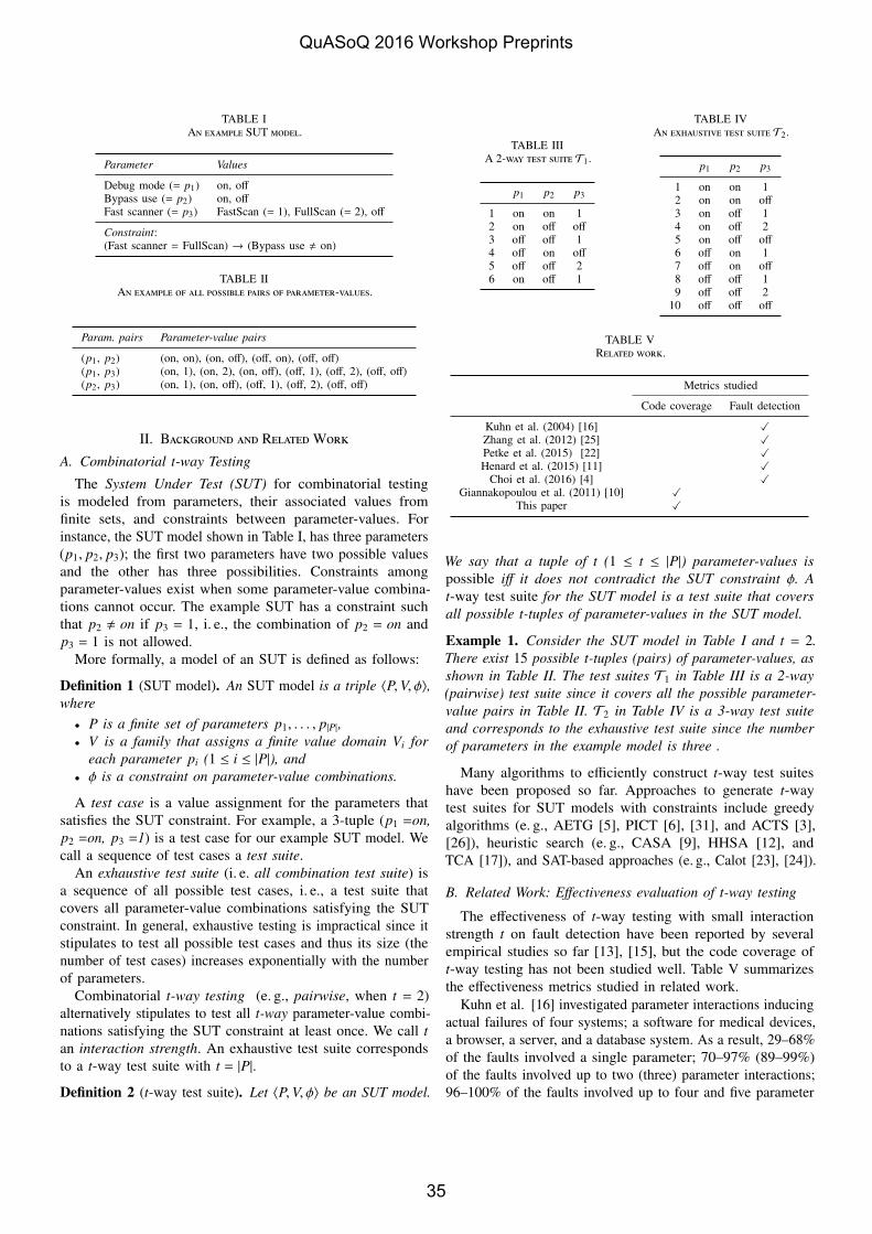
TABLE IAn example SUT model.

Parameter Values

Debug mode (= p1) on, o↵Bypass use (= p2) on, o↵Fast scanner (= p3) FastScan (= 1), FullScan (= 2), o↵

Constraint:(Fast scanner = FullScan) ! (Bypass use , on)

TABLE IIAn example of all possible pairs of parameter-values.

Param. pairs Parameter-value pairs

(p1, p2) (on, on), (on, o↵), (o↵, on), (o↵, o↵)(p1, p3) (on, 1), (on, 2), (on, o↵), (o↵, 1), (o↵, 2), (o↵, o↵)(p2, p3) (on, 1), (on, o↵), (o↵, 1), (o↵, 2), (o↵, o↵)

II. Background and RelatedWorkA. Combinatorial t-way Testing

The System Under Test (SUT) for combinatorial testingis modeled from parameters, their associated values fromfinite sets, and constraints between parameter-values. Forinstance, the SUT model shown in Table I, has three parameters(p1, p2, p3); the first two parameters have two possible valuesand the other has three possibilities. Constraints amongparameter-values exist when some parameter-value combina-tions cannot occur. The example SUT has a constraint suchthat p2 , on if p3 = 1, i. e., the combination of p2 = on andp3 = 1 is not allowed.

More formally, a model of an SUT is defined as follows:

Definition 1 (SUT model). An SUT model is a triple hP,V, �i,where

• P is a finite set of parameters p1, . . . , p|P|,• V is a family that assigns a finite value domain V

i

for

each parameter p

i

(1 i |P|), and

• � is a constraint on parameter-value combinations.

A test case is a value assignment for the parameters thatsatisfies the SUT constraint. For example, a 3-tuple (p1 =on,

p2 =on, p3 =1) is a test case for our example SUT model. Wecall a sequence of test cases a test suite.

An exhaustive test suite (i. e. all combination test suite) isa sequence of all possible test cases, i. e., a test suite thatcovers all parameter-value combinations satisfying the SUTconstraint. In general, exhaustive testing is impractical since itstipulates to test all possible test cases and thus its size (thenumber of test cases) increases exponentially with the numberof parameters.

Combinatorial t-way testing (e. g., pairwise, when t = 2)alternatively stipulates to test all t-way parameter-value combi-nations satisfying the SUT constraint at least once. We call t

an interaction strength. An exhaustive test suite correspondsto a t-way test suite with t = |P|.Definition 2 (t-way test suite). Let hP,V, �i be an SUT model.

TABLE IIIA 2-way test suite T1.

p1 p2 p3

1 on on 12 on o↵ o↵3 o↵ o↵ 14 o↵ on o↵5 o↵ o↵ 26 on o↵ 1

TABLE IVAn exhaustive test suite T2.

p1 p2 p3

1 on on 12 on on o↵3 on o↵ 14 on o↵ 25 on o↵ o↵6 o↵ on 17 o↵ on o↵8 o↵ o↵ 19 o↵ o↵ 2

10 o↵ o↵ o↵

TABLE VRelated work.

Metrics studied

Code coverage Fault detection

Kuhn et al. (2004) [16] XZhang et al. (2012) [25] XPetke et al. (2015) [22] XHenard et al. (2015) [11] X

Choi et al. (2016) [4] XGiannakopoulou et al. (2011) [10] X

This paper X

We say that a tuple of t (1 t |P|) parameter-values is

possible i↵ it does not contradict the SUT constraint �. A

t-way test suite for the SUT model is a test suite that covers

all possible t-tuples of parameter-values in the SUT model.

Example 1. Consider the SUT model in Table I and t = 2.

There exist 15 possible t-tuples (pairs) of parameter-values, as

shown in Table II. The test suites T1 in Table III is a 2-way

(pairwise) test suite since it covers all the possible parameter-

value pairs in Table II. T2 in Table IV is a 3-way test suite

and corresponds to the exhaustive test suite since the number

of parameters in the example model is three .

Many algorithms to e�ciently construct t-way test suiteshave been proposed so far. Approaches to generate t-waytest suites for SUT models with constraints include greedyalgorithms (e. g., AETG [5], PICT [6], [31], and ACTS [3],[26]), heuristic search (e. g., CASA [9], HHSA [12], andTCA [17]), and SAT-based approaches (e. g., Calot [23], [24]).

B. Related Work: E↵ectiveness evaluation of t-way testing

The e↵ectiveness of t-way testing with small interactionstrength t on fault detection have been reported by severalempirical studies so far [13], [15], but the code coverage oft-way testing has not been studied well. Table V summarizesthe e↵ectiveness metrics studied in related work.

Kuhn et al. [16] investigated parameter interactions inducingactual failures of four systems; a software for medical devices,a browser, a server, and a database system. As a result, 29–68%of the faults involved a single parameter; 70–97% (89–99%)of the faults involved up to two (three) parameter interactions;96–100% of the faults involved up to four and five parameter


35

interactions; no fault involved more than six parameters. Fromthe result, the authors concluded that most failures are triggeredby parameter interactions with small t (at most four to six)and thus t-way testing with 4 t 6 could provide the faultdetection ability of “pseudo-exhaustive” testing.

Zhang et al. [25] also explored that failures of actualcommercial MP3 players are triggered by t-way parameterinteractions with at most t = 4.

Petke et al. [22] more thoroughly studied the e�ciency ofearly fault detection by t-way testing with 2 t 6. Theyused six projects, flex, make, grep, gzip, nanoxml, and siena,from the Software artifact Infrastructure Repository (SIR) andshowed the number of faults detected after 25%, 50%, 70%,and 100% of test cases are executed.

Henard et al. [11] used five projects, grep, sed, flex, make,and gzip, also from SIR and compared the number of faultsdetected by test suite prioritization with t-way coverage (2 t 4) and other black-box and white-box prioritization.

Choi et al. [4] used three projects, flex, grep, and make,from SIR and investigated a correlation of the fault detection ef-fectiveness with two evaluation metrics, called weight coverageand KL divergence, for prioritized t (= 2)-way testing.

To our knowledge, the only work by Giannakopoulou etal. [10] reported code coverage of t-way testing. Their targetsystem is a component of the Tactical Separation AssistedFlight Environment (TSAFE) of the Next Generation AirTransportation System (NextGen) by the NASA Ames ResearchCenter. In their work, t (= 3)-way testing and their model-checker (JPF [30]) based exhaustive testing are comparedw. r. t. code coverage; line coverage, branch coverage, loopcoverage, and strict condition coverage, which are computedusing CodeCover [28].

Giannakopoulou et al. reported that for two program mod-ules, the di↵erences of code coverage by 3-way testing andexhaustive testing are 0–2% for the four coverage metrics theyused, while the numbers of test cases are 6,047 for 3-waytesting but 9.9 ⇥ 106 for exhaustive testing. In this paper, wemore thoroughly analyze the code coverage e↵ectiveness oft-way testing with 1 t 4 using three open source utilityprograms.

III. Experiments

A. Subject Programs

To investigate code coverage of t-way testing, we use threeopen source projects of C programs, flex, grep, and make,from the Software artifact Infrastructure Repository (SIR) [32].flex is a lexical analysis generator. grep is a program to searchfor text matching regular expressions. make is a program tocontrol the compile and build process. The programs havebeen widely used to evaluate testing techniques by researchersin studies including [4], [11], [22]. Table VI shows for eachversion of programs we use, the version identifier, the yearreleased, and the lines of code (LoC) calculated using cloc [27].

TABLE VISubject programs.

Proj. Ver. Identifier Year of release LoC

flex

v0 2.4.3 1993 10,163v1 2.4.7 1994 10,546v2 2.5.1 1995 13,000v3 2.5.2 1996 13,048v4 2.5.3 1996 13,142v5 2.5.4 1997 13,144

grep

v0 2.0 1996 8,163v1 2.2 1998 11,945v2 2.3 1999 12,681v3 2.4 1999 12,780v4 2.4.1 2000 13,280v5 2.4.2 2000 13,275

make

v0 3.75 1996 17,424v1 3.76.1 1997 18,525v2 3.77 1998 19,610v3 3.78.1 1999 20,401v4 3.79.1 2000 23,188

Parameters:

...

Debug mode: # -d

Debug_on.

Debug_off.

Bypass use: # -Cr

Bypass_on. [property Bypass]

Bypass_off.

Fast scanner: # -f, -Cf

FastScan. [property FastScan]

FullScan. [if !Bypass][property FullScan]

off. [property f&Cfoff]

...

Fig. 1. A part of the test plan for flex in TSL.

B. Subject Test Suites

1) SUT Models: For each project, flex, grep, and make, weconstruct an SUT model for t-way testing whose parameters,values, and constraints are fully extracted from the test plan inTSL (Test Specification Language), which is included in SIR.For example, Figure 1 shows a part of the test plan in TSL forproject flex. From the TSL specification, we construct the SUTmodel for flex whose parameters include Debug mode(= p1),Bypass use(= p2) and Fast scanner(= p3), p2 has two valuesincluding Bypass on(= on), p3 has three values includingFullScan(= 2), and constraints include (p3 = 2)! (p2 , on).Table I corresponds to a part of the SUT model for flex, whichis constructed from the part of the test plan in Figure 1.

Table VII shows the size of the SUT model constructedfor each project. In the table, the size of parameter-values isexpressed as k; g

k11 g

k22 . . . g

k

n

n

, which indicates that the number ofparameters is k and for each i there are k

i

parameters that haveg

i

values. The size of constraints is expressed as l; l

h11 l

h22 . . . l

h

m

m

,which indicates that the constraint is described in conjunctivenormal form (CNF) with l variables whose Boolean value


36

TABLE VIIConstructed SUT models.

Proj. Model size

flex

Parameter-values 29; 3234462

Constraints 97; 27122212422517269

grep


Constraints 87; 243332748751612412712813110

make


Constraints 79; 2526211221231243257269

TABLE VIIISizes and code coverage of exhaustive test suites.

Proj. Size Line coverage Branch coverage

flex 525Avg. 0.7968 0.8544Min. 0.7789 0.8151Max. 0.8312 0.9316

grep 470Avg. 0.4961 0.4948Min. 0.4726 0.4746Max. 0.5900 0.5826

make 793Avg. 0.4543 0.5373Min. 0.4234 0.5126Max. 0.4726 0.5494

represents an assignment of a value to a parameter and foreach j there are h

j

clauses that have l

j

literals. For the exampleSUT model in Figure 1, the size of parameter-values is 3; 2231

and the size of constraints is 2; 21.2) Test Suites: We use t-way test suites with 1 t 4 that

are generated by ACTS [3], [26] and PICT [6], [31] for ourconstructed SUT models with constraints. The tools ACTS andPICT are state-of-the-art open source t-way test generationtools developed by NIST (National Institute of Standards andTechnology) and Microsoft, respectively. For comparison, wealso use exhaustive test suites each of which obtains all possibletest cases. The exhaustive test suite for the test plan of eachproject is included in SIR.

3) Evaluation Metrics: To evaluate code coverage of eachtest suite, we analyze the following two kinds of code coverage,which are computed using gcov [29]:• Line coverage: the percentage of program lines executed.• Branch coverage: the percentage of branches of conditional

statements executed.gcov is a source code analysis tool, which is a standard utilitydelivered with the GNU C/C++ Compiler and reports howmany lines and branches are executed.

IV. ResultsTable VIII shows the size, i. e. the number of test cases,

and the code coverage (line coverage and branch coverage) ofthe exhaustive test suite for each project, while Table IX andTable X show those of the subject t-way test suites (1 t 4)generated by ACTS and PICT. Table IX shows the sizes of thesubject t-way test suites with the ratio of them over the sizes ofexhaustive test suites. Table X summarizes line coverage andbranch coverage of the subject t-way test suites for each project.

Line Branch

●

● ● ●

●●●●

●

●

●●

0.96

0.97

0.98

0.99

1.00

1−way 2−way 3−way 4−way 1−way 2−way 3−way 4−way

Fig. 2. Ratio of code coverage of t-way testing (1 t 4) over that ofexhaustive testing for all versions of projects.

Line Branch

0.2

0.3

0.4

0.5

0 100 200 300 400 0 100 200 300 400Test cases

1−way2−way3−way4−wayExhaustive

Fig. 3. Example code coverage growths of t-way testing (1 t 4) andexhaustive testing for one version (v1) of grep.

In Table VIII and Table X, we show the average, minimum,and maximum values of code coverage for versions of eachproject.

For example, for project flex, the sizes of 2-way test suites(52 by ACTS and 51 by PICT) are less than 10% of the sizeof the exhaustive test suite (525) from Table VIII and Table IX.On the other hand, for flex, line coverage and branch coverageof 2-way test suites (the exhaustive test suite) are on average0.7927 (0.7968) and 0.8522 (0.8544) from Table VIII andTable X.

A. RQ1: t-way testing vs. exhaustive testing

To compare the code coverage between t-way testing andexhaustive testing, we investigate the following metric

R

Cov

(Tt

, EX) = Cov(Tt

) / Cov(EX),

which denotes the ratio of code coverage of t-way test suiteT

t

over that of exhaustive test suite EX.Table XI summarizes the values of R

Cov

(Tt

, EX) with 1 t 4 for line coverage and branch coverage for each project and


37

TABLE IXSizes of t-way test suites (1 t 4).

Proj. # of test cases (ratio over # of the exhaustive test cases)

1-way 2-way 3-way 4-way

flex

ACTS 30 (5.71 %) 52 (9.90 %) 91 (17.33 %) 155 (29.52 %)PICT 30 (5.71 %) 51 (9.71 %) 90 (17.14 %) 154 (29.33 %)

grep

ACTS 40 (8.51 %) 76 (16.17 %) 183 (38.94 %) 328 (69.79 %)PICT 40 (8.51 %) 77 (16.38 %) 180 (38.30 %) 326 (69.36 %)

make

ACTS 27 (3.40 %) 34 (4.29 %) 44 (5.55 %) 68 (8.58 %)PICT 27 (3.40 %) 34 (4.29 %) 45 (5.67 %) 69 (8.70 %)

TABLE XCode coverage of t-way test suites (1 t 4).

Proj. Line coverage Branch coverage

1-way 2-way 3-way 4-way 1-way 2-way 3-way 4-way

flex

Avg. 0.7683 0.7927 0.7934 0.7931 0.8407 0.8522 0.8522 0.8522Min. 0.7481 0.7755 0.7763 0.7755 0.8018 0.8136 0.8136 0.8136Max. 0.8145 0.8264 0.8267 0.8267 0.9225 0.9281 0.9281 0.9281

grep

Avg. 0.4917 0.4959 0.4961 0.4961 0.4769 0.4880 0.4933 0.4948Min. 0.4668 0.4723 0.4726 0.4726 0.4549 0.4676 0.4712 0.4746Max. 0.5875 0.5897 0.5900 0.5900 0.5726 0.5786 0.5845 0.5826

make

Avg. 0.4451 0.4539 0.4540 0.4540 0.5321 0.5364 0.5366 0.5366Min. 0.4168 0.4230 0.4230 0.4230 0.5053 0.5117 0.5117 0.5117Max. 0.4628 0.4724 0.4724 0.4726 0.5442 0.5484 0.5484 0.5484

TABLE XIComparison of code coverage between t-way testing (1 t 4) and exhaustive testing.



flex 96.41 % 99.49 % 99.58 % 99.54 % 98.40 % 99.74 % 99.74 % 99.74 %Avg. of R

Cov

(Tt

, EX) grep 99.11 % 99.95 % 100.00 % 100.00 % 96.32 % 98.58 % 99.67 % 100.00 %(R = Cov(T

t

)/Cov(EX)) make 97.97 % 99.91 % 99.93 % 99.92 % 99.03 % 99.84 % 99.88 % 99.87 %Avg. 97.82 % 99.77 % 99.83 % 99.81 % 97.85 % 99.36 % 99.76 % 99.87 %

flex 0 / 12 8 / 12 8 / 12 8 / 12 0 / 12 12 / 12 12 / 12 12 / 12# (R � 99.5 %) grep 4 / 12 12 / 12 12 / 12 12 / 12 0 / 12 0 / 12 7 / 12 12 / 12/ # all cases make 0 / 10 10 / 10 10 / 10 10 / 10 0 / 10 10 / 10 10 / 10 10 / 10

Total 4 / 34 30 / 34 30 / 34 30 / 34 0 / 34 22 / 34 29 / 34 34 / 34

all projects. In the table, we also show the numbers of caseswhere R

Cov

(Tt

, EX) � 99.5%, i. e. t-way testing achieves morethan 99.5% of the coverage obtained by exhaustive testing,over the numbers of all cases (versions) for projects.

Figure 2 presents the box plots for the results of R

Cov

(Tt

, EX)for all projects. Each box plot shows the mean (circle in thebox), median (thick horizontal line), the first/third quartiles(hinges), and highest/lowest values within 1.5 ⇥ the inter-quartile range of the hinge (whiskers).• How high code coverage can t-way testing achieve

compared to exhaustive testing?From Table XI and Figure 2, we can see that t-way testing

with even small t can achieve high values of R

Cov

(Tt

, EX),i. e. high ratios of code coverage over the code coverage ofexhaustive testing.

In the result of our case study, 1-way (2-way) testing coversavg. 97.82% (99.77%) of line coverage of exhaustive testing and

avg. 97.85% (99.36%) of branch coverage of exhaustive testing.With 3-way (4-way) testing, line coverage is avg. 99.83%(99.81%) and branch coverage is avg. 99.76% (99.87%) of thecoverage of exhaustive testing.• Can t-way testing obtain higher code coverage earlier

compared to exhaustive testing?Figure 3 shows example line coverage growths and branch

coverage growths of t-way test suites (1 t 4) and theexhaustive test suites for one version (v1) of project grep. (Thecoverage growths represent the typical cases of our experimentresults.) We can see that t-way testing with smaller t obtainshigher code coverage earlier compared to exhaustive testingand t-way testing with larger t.

For the example case in Figure 3, to obtain 48% line coverage(46% branch coverage), 1-way, 2-way, 3-way, and 4-way testingrespectively require 35, 42, 56, and 56 (36, 47, 71, and 71) testcases, while exhaustive testing requires 219 (265) test cases.


38

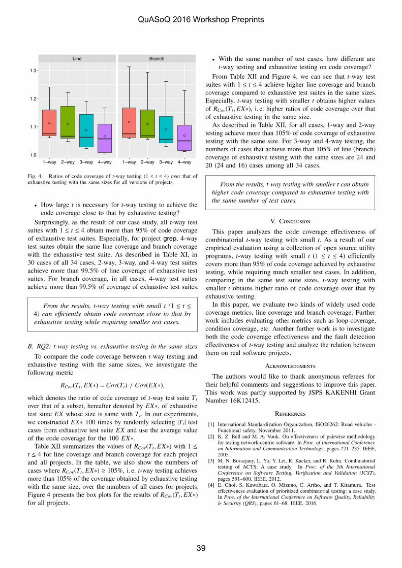
Line Branch

● ●

●

●

●●

●

●

1.0

1.1

1.2

1.3

1−way 2−way 3−way 4−way 1−way 2−way 3−way 4−way

Fig. 4. Ratios of code coverage of t-way testing (1 t 4) over that ofexhaustive testing with the same sizes for all versions of projects.

• How large t is necessary for t-way testing to achieve thecode coverage close to that by exhaustive testing?

Surprisingly, as the result of our case study, all t-way testsuites with 1 t 4 obtain more than 95% of code coverageof exhaustive test suites. Especially, for project grep, 4-waytest suites obtain the same line coverage and branch coveragewith the exhaustive test suite. As described in Table XI, in30 cases of all 34 cases, 2-way, 3-way, and 4-way test suitesachieve more than 99.5% of line coverage of exhaustive testsuites. For branch coverage, in all cases, 4-way test suitesachieve more than 99.5% of coverage of exhaustive test suites.

From the results, t-way testing with small t (1 t 4) can e�ciently obtain code coverage close to that by

exhaustive testing while requiring smaller test cases.

B. RQ2: t-way testing vs. exhaustive testing in the same sizes

To compare the code coverage between t-way testing andexhaustive testing with the same sizes, we investigate thefollowing metric

R

Cov

(Tt

, EX⇤) = Cov(Tt

) / Cov(EX⇤),which denotes the ratio of code coverage of t-way test suite T

t

over that of a subset, hereafter denoted by EX⇤, of exhaustivetest suite EX whose size is same with T

t

. In our experiments,we constructed EX⇤ 100 times by randomly selecting |T

t

| testcases from exhaustive test suite EX and use the average valueof the code coverage for the 100 EX⇤.

Table XII summarizes the values of R

Cov

(Tt

, EX⇤) with 1 t 4 for line coverage and branch coverage for each projectand all projects. In the table, we also show the numbers ofcases where R

Cov

(Tt

, EX⇤) � 105%, i. e. t-way testing achievesmore than 105% of the coverage obtained by exhaustive testingwith the same size, over the numbers of all cases for projects.Figure 4 presents the box plots for the results of R

Cov

(Tt

, EX⇤)for all projects.

• With the same number of test cases, how di↵erent aret-way testing and exhaustive testing on code coverage?

From Table XII and Figure 4, we can see that t-way testsuites with 1 t 4 achieve higher line coverage and branchcoverage compared to exhaustive test suites in the same sizes.Especially, t-way testing with smaller t obtains higher valuesof R

Cov

(Tt

, EX⇤), i. e. higher ratios of code coverage over thatof exhaustive testing in the same size.

As described in Table XII, for all cases, 1-way and 2-waytesting achieve more than 105% of code coverage of exhaustivetesting with the same size. For 3-way and 4-way testing, thenumbers of cases that achieve more than 105% of line (branch)coverage of exhaustive testing with the same sizes are 24 and20 (24 and 16) cases among all 34 cases.

From the results, t-way testing with smaller t can obtain

higher code coverage compared to exhaustive testing with

the same number of test cases.

V. ConclusionThis paper analyzes the code coverage e↵ectiveness of

combinatorial t-way testing with small t. As a result of ourempirical evaluation using a collection of open source utilityprograms, t-way testing with small t (1 t 4) e�cientlycovers more than 95% of code coverage achieved by exhaustivetesting, while requiring much smaller test cases. In addition,comparing in the same test suite sizes, t-way testing withsmaller t obtains higher ratio of code coverage over that byexhaustive testing.

In this paper, we evaluate two kinds of widely used codecoverage metrics, line coverage and branch coverage. Furtherwork includes evaluating other metrics such as loop coverage,condition coverage, etc. Another further work is to investigateboth the code coverage e↵ectiveness and the fault detectione↵ectiveness of t-way testing and analyze the relation betweenthem on real software projects.

AcknowledgmentsThe authors would like to thank anonymous referees for

their helpful comments and suggestions to improve this paper.This work was partly supported by JSPS KAKENHI GrantNumber 16K12415.

References[1] International Standardization Organization, ISO26262: Road vehicles -

Functional safety, November 2011.[2] K. Z. Bell and M. A. Vouk. On e↵ectiveness of pairwise methodology

for testing network-centric software. In Proc. of International Conference

on Information and Communication Technology, pages 221–235. IEEE,2005.

[3] M. N. Borazjany, L. Yu, Y. Lei, R. Kacker, and R. Kuhn. Combinatorialtesting of ACTS: A case study. In Proc. of the 5th International

Conference on Software Testing, Verification and Validation (ICST),pages 591–600. IEEE, 2012.

[4] E. Choi, S. Kawabata, O. Mizuno, C. Artho, and T. Kitamura. Teste↵ectiveness evaluation of prioritized combinatorial testing: a case study.In Proc. of the International Conference on Software Quality, Reliability

& Security (QRS), pages 61–68. IEEE, 2016.


39

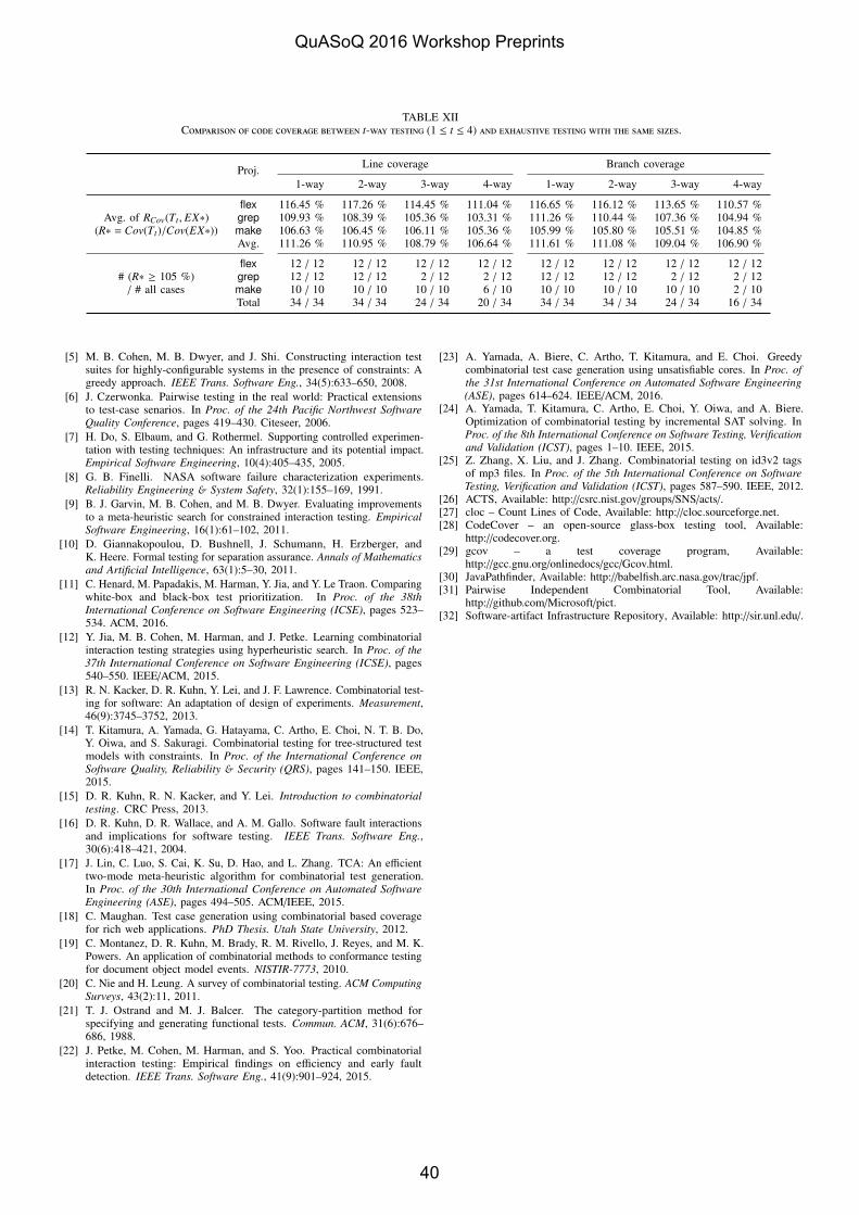
TABLE XIIComparison of code coverage between t-way testing (1 t 4) and exhaustive testing with the same sizes.



flex 116.45 % 117.26 % 114.45 % 111.04 % 116.65 % 116.12 % 113.65 % 110.57 %Avg. of R

Cov

(Tt

, EX⇤) grep 109.93 % 108.39 % 105.36 % 103.31 % 111.26 % 110.44 % 107.36 % 104.94 %(R⇤ = Cov(T

t

)/Cov(EX⇤)) make 106.63 % 106.45 % 106.11 % 105.36 % 105.99 % 105.80 % 105.51 % 104.85 %Avg. 111.26 % 110.95 % 108.79 % 106.64 % 111.61 % 111.08 % 109.04 % 106.90 %

flex 12 / 12 12 / 12 12 / 12 12 / 12 12 / 12 12 / 12 12 / 12 12 / 12# (R⇤ � 105 %) grep 12 / 12 12 / 12 2 / 12 2 / 12 12 / 12 12 / 12 2 / 12 2 / 12/ # all cases make 10 / 10 10 / 10 10 / 10 6 / 10 10 / 10 10 / 10 10 / 10 2 / 10

Total 34 / 34 34 / 34 24 / 34 20 / 34 34 / 34 34 / 34 24 / 34 16 / 34

[5] M. B. Cohen, M. B. Dwyer, and J. Shi. Constructing interaction testsuites for highly-configurable systems in the presence of constraints: Agreedy approach. IEEE Trans. Software Eng., 34(5):633–650, 2008.

[6] J. Czerwonka. Pairwise testing in the real world: Practical extensionsto test-case senarios. In Proc. of the 24th Pacific Northwest Software

Quality Conference, pages 419–430. Citeseer, 2006.[7] H. Do, S. Elbaum, and G. Rothermel. Supporting controlled experimen-

tation with testing techniques: An infrastructure and its potential impact.Empirical Software Engineering, 10(4):405–435, 2005.

[8] G. B. Finelli. NASA software failure characterization experiments.Reliability Engineering & System Safety, 32(1):155–169, 1991.

[9] B. J. Garvin, M. B. Cohen, and M. B. Dwyer. Evaluating improvementsto a meta-heuristic search for constrained interaction testing. Empirical

Software Engineering, 16(1):61–102, 2011.[10] D. Giannakopoulou, D. Bushnell, J. Schumann, H. Erzberger, and

K. Heere. Formal testing for separation assurance. Annals of Mathematics

and Artificial Intelligence, 63(1):5–30, 2011.[11] C. Henard, M. Papadakis, M. Harman, Y. Jia, and Y. Le Traon. Comparing

white-box and black-box test prioritization. In Proc. of the 38th

International Conference on Software Engineering (ICSE), pages 523–534. ACM, 2016.

[12] Y. Jia, M. B. Cohen, M. Harman, and J. Petke. Learning combinatorialinteraction testing strategies using hyperheuristic search. In Proc. of the

37th International Conference on Software Engineering (ICSE), pages540–550. IEEE/ACM, 2015.

[13] R. N. Kacker, D. R. Kuhn, Y. Lei, and J. F. Lawrence. Combinatorial test-ing for software: An adaptation of design of experiments. Measurement,46(9):3745–3752, 2013.

[14] T. Kitamura, A. Yamada, G. Hatayama, C. Artho, E. Choi, N. T. B. Do,Y. Oiwa, and S. Sakuragi. Combinatorial testing for tree-structured testmodels with constraints. In Proc. of the International Conference on

Software Quality, Reliability & Security (QRS), pages 141–150. IEEE,2015.

[15] D. R. Kuhn, R. N. Kacker, and Y. Lei. Introduction to combinatorial

testing. CRC Press, 2013.[16] D. R. Kuhn, D. R. Wallace, and A. M. Gallo. Software fault interactions

and implications for software testing. IEEE Trans. Software Eng.,30(6):418–421, 2004.

[17] J. Lin, C. Luo, S. Cai, K. Su, D. Hao, and L. Zhang. TCA: An e�cienttwo-mode meta-heuristic algorithm for combinatorial test generation.In Proc. of the 30th International Conference on Automated Software

Engineering (ASE), pages 494–505. ACM/IEEE, 2015.[18] C. Maughan. Test case generation using combinatorial based coverage

for rich web applications. PhD Thesis. Utah State University, 2012.[19] C. Montanez, D. R. Kuhn, M. Brady, R. M. Rivello, J. Reyes, and M. K.

Powers. An application of combinatorial methods to conformance testingfor document object model events. NISTIR-7773, 2010.

[20] C. Nie and H. Leung. A survey of combinatorial testing. ACM Computing

Surveys, 43(2):11, 2011.[21] T. J. Ostrand and M. J. Balcer. The category-partition method for

specifying and generating functional tests. Commun. ACM, 31(6):676–686, 1988.

[22] J. Petke, M. Cohen, M. Harman, and S. Yoo. Practical combinatorialinteraction testing: Empirical findings on e�ciency and early faultdetection. IEEE Trans. Software Eng., 41(9):901–924, 2015.

[23] A. Yamada, A. Biere, C. Artho, T. Kitamura, and E. Choi. Greedycombinatorial test case generation using unsatisfiable cores. In Proc. of

the 31st International Conference on Automated Software Engineering

(ASE), pages 614–624. IEEE/ACM, 2016.[24] A. Yamada, T. Kitamura, C. Artho, E. Choi, Y. Oiwa, and A. Biere.

Optimization of combinatorial testing by incremental SAT solving. InProc. of the 8th International Conference on Software Testing, Verification

and Validation (ICST), pages 1–10. IEEE, 2015.[25] Z. Zhang, X. Liu, and J. Zhang. Combinatorial testing on id3v2 tags

of mp3 files. In Proc. of the 5th International Conference on Software

Testing, Verification and Validation (ICST), pages 587–590. IEEE, 2012.[26] ACTS, Available: http://csrc.nist.gov/groups/SNS/acts/.[27] cloc – Count Lines of Code, Available: http://cloc.sourceforge.net.[28] CodeCover – an open-source glass-box testing tool, Available:

http://codecover.org.[29] gcov – a test coverage program, Available:

http://gcc.gnu.org/onlinedocs/gcc/Gcov.html.[30] JavaPathfinder, Available: http://babelfish.arc.nasa.gov/trac/jpf.[31] Pairwise Independent Combinatorial Tool, Available:

http://github.com/Microsoft/pict.[32] Software-artifact Infrastructure Repository, Available: http://sir.unl.edu/.


40

Sustainability Profiling ofLong-living Software Systems

Ahmed D. Alharthi, Maria Spichkova and Margaret HamiltonRMIT University, Melbourne, Australia

Email: {ahmed.alharthi, maria.spichkova,margaret.hamilton}@rmit.edu.au

Abstract—This paper introduces a framework for softwaresustainability profiling. The goal of the framework is to analysesustainability requirements for long-living software systems, fo-cusing on usability and readability of the sustainability profiles.To achieve this goal, we apply a quantitate approach such asfuzzy rating scale-based questionnaires to rank the sustainabil-ity requirements, and the Technique for Order Preference bySimilarity to Ideal Solution (TOPSIS) to analyse the results ofquestionnaires and to provide a basis for system profiling.

The core profiling elements provided by our framework are(1) a sustainability five-star rating, (2) visualisation of the fivesustainability dimensions as a pentagon graph detailing combina-tion for individual, social, technical, economic and environmentaldimensions, and (3) a bar graph of overall sustainability level foreach requirement. To ensure sustainability, the proposed profilingframework covers the five dimensions of sustainability to quantifythe sustainability of any software system not only during therequirement gathering phase but also during maintenance phaseof software system lifecycle.

I. INTRODUCTION

Addressing the impacts of software systems on sustainabil-ity is a first-class quality concern beside usability, safety andsecurity [1]. A number of studies showed that if a softwaresystem is developed without taking sustainability requirementsinto account, the system could have negative impacts onindividual, social, technology, economic, and environmentsustainability, cf. [2]–[5]. Environmental awareness is crucialfor software engineering, especially in the case of large-scalesystems having many thousands of users.

The analysis of system sustainability has to be initiated onthe requirements engineering (RE) phase [6], [7]. Based onthis idea, Becker et al. [8] emphasised that the importance ofidentifying stakeholders whose outside interests are affected,and the use of long-life scenarios techniques during require-ments elicitation could forecast potential impacts. Duffy [9]highlighted that sustainability could be achieved especiallyin the social dimension through usability, which is a non-functional requirement, and its traditional methodologies.

This question is especially important for long-living sys-tems, where the stakeholders requirements and preferencesmight change over the time the system is in use. For example,a system that can be seen as sustainable today, might berated as environmentally unsustainable in few years, whilenew techniques to increase environmental sustainability aredeveloped. To solve this problem, we require an easy-to-useprofiling framework based on quantitate approaches that wouldallow to analyse the up-to-date system sustainability profiles,

based on system characteristics and the up-to-date ratings(quotations) of the corresponding requirements. Usability andreadability of the approach is crucial to make it applicablefor real software development processes, as the quotationprocess and the generated profiles have to be easy-to-use byall stakeholders.

Contributions: To ensure the sustainability of long-livingsoftware systems over their eitire live-cycle, we propose aframework for sustainability profiling. The framework allowsto analyse sustainability requirements for long-living softwaresystems. The up-to-date profiles could be generated bothduring the RE and the maintenance phase of the softwaresystem lifecycle. The framework workflow is presented inFigure 1. First of all, stakeholders are assigned to a groupto rate requirements from the different perspective of sus-tainability dimensions (individual, social, technical, economicand environmental). Then, a fuzzy rating scale is used toavoid imprecision for answering quantitative questionnaires[10]. As the next step, the Technique for Order of Preferenceby Similarity to Ideal Solution (TOPSIS, cf. [11]) is utilisedto find alternatives that are the nearest distance from thepositive ideal solution and farthest distance from the negativeideal solution. The software sustainability profiling includesan overall picture of how sustainable a software system reallyis. The profile is presented as three core elements: (1) a five-star rating, (2) five dimensions of sustainability in a pentagongraph, and (4) an overall measure of sustainability for eachrequirement in a bar graph.

Outline: The rest of the paper is organised as follows. InSection II we discuss the background and related work. Sec-tion III introduces our framework for software sustainabilityprofiling. Section IV introduces an example scenario to showhow the framework can be used to profile software systems.Section V summarises the core contributions of our work.

II. BACKGROUND AND RELATED WORK

In this section we discuss the research directions andapproaches that provide a background for our framework: REfor sustainable systems, the idea of the sustainability profiling,quantitative approaches, approaches using the fuzzy ratingscale, and the TOPSIS framework for requirements analysis.We selected TOPSIS for our sustainability profiling frame-work, as this technique has been successfully used for priori-tising requirements and solving conflict among non-functionalrequirements, cf. [11]–[13]. Previously, TOPSIS was used


41

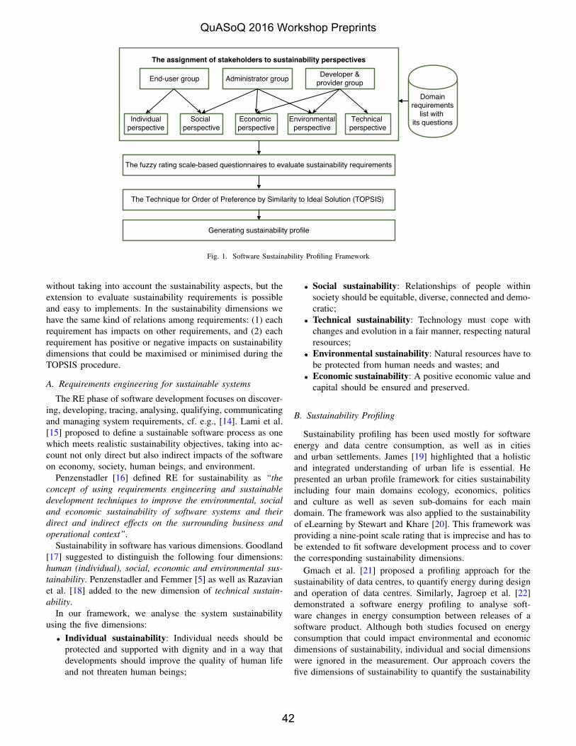
Fig. 1. Software Sustainability Profiling Framework

without taking into account the sustainability aspects, but theextension to evaluate sustainability requirements is possibleand easy to implements. In the sustainability dimensions wehave the same kind of relations among requirements: (1) eachrequirement has impacts on other requirements, and (2) eachrequirement has positive or negative impacts on sustainabilitydimensions that could be maximised or minimised during theTOPSIS procedure.

A. Requirements engineering for sustainable systems

The RE phase of software development focuses on discover-ing, developing, tracing, analysing, qualifying, communicatingand managing system requirements, cf. e.g., [14]. Lami et al.[15] proposed to define a sustainable software process as onewhich meets realistic sustainability objectives, taking into ac-count not only direct but also indirect impacts of the softwareon economy, society, human beings, and environment.

Penzenstadler [16] defined RE for sustainability as “theconcept of using requirements engineering and sustainabledevelopment techniques to improve the environmental, socialand economic sustainability of software systems and theirdirect and indirect effects on the surrounding business andoperational context”.

Sustainability in software has various dimensions. Goodland[17] suggested to distinguish the following four dimensions:human (individual), social, economic and environmental sus-tainability. Penzenstadler and Femmer [5] as well as Razavianet al. [18] added to the new dimension of technical sustain-ability.

In our framework, we analyse the system sustainabilityusing the five dimensions:• Individual sustainability: Individual needs should be

protected and supported with dignity and in a way thatdevelopments should improve the quality of human lifeand not threaten human beings;

• Social sustainability: Relationships of people withinsociety should be equitable, diverse, connected and demo-cratic;

• Technical sustainability: Technology must cope withchanges and evolution in a fair manner, respecting naturalresources;

• Environmental sustainability: Natural resources have tobe protected from human needs and wastes; and

• Economic sustainability: A positive economic value andcapital should be ensured and preserved.

B. Sustainability Profiling

Sustainability profiling has been used mostly for softwareenergy and data centre consumption, as well as in citiesand urban settlements. James [19] highlighted that a holisticand integrated understanding of urban life is essential. Hepresented an urban profile framework for cities sustainabilityincluding four main domains ecology, economics, politicsand culture as well as seven sub-domains for each maindomain. The framework was also applied to the sustainabilityof eLearning by Stewart and Khare [20]. This framework wasproviding a nine-point scale rating that is imprecise and has tobe extended to fit software development process and to coverthe corresponding sustainability dimensions.

Gmach et al. [21] proposed a profiling approach for thesustainability of data centres, to quantify energy during designand operation of data centres. Similarly, Jagroep et al. [22]demonstrated a software energy profiling to analyse soft-ware changes in energy consumption between releases of asoftware product. Although both studies focused on energyconsumption that could impact environmental and economicdimensions of sustainability, individual and social dimensionswere ignored in the measurement. Our approach covers thefive dimensions of sustainability to quantify the sustainability


42

of any software system, starting from the requirements phaseand continuing over the phase of maintenance.

C. Quantitative Approach

Quantitative approaches are used to analyse data and to mea-sure qualities in software engineering [23], [24]. For instance,goal-oriented requirements and user experience are analysedand measured via quantitative techniques having a rating scaleof probability between satisfaction and denial of satisfaction.The rating scales and data analysis techniques vary from onequantitative approach to another. Some approaches use a five-level Likert scale while others employ a nine-point scale topresent people’s attitudes by scaling their responses. Notably,the Likert rating scales and the nine scales that are givinga number of options are closed format. For example, if aquestionnaire has a closed five Likert scale, participants canonly express their opinion through one of the five choices.These closed format options are imprecise, difficult to choosebetween and limited. A solution to overcome drawbacks ofclosed formatted scales are the fuzzy rating scale [10], cf.Section II-D for more details.

The quantitate approaches can be applied to several types ofdata, and the type of data to analyse might influence the choiceof the approach. Tullis and Albert [23] suggest to distinguishthe following four types of data:• Nominal data is categorised or classification data, which

it is not in any particular order, e.g., gender or hair colour;• Ordinal data is ordered classified data, but the differ-

ences between them are not meaningful, e.g., product andmovie ratings;

• Interval data is classified data where the differencebetween two data items is meaningful, but without naturalzero points, e.g., temperature units;

• Ratio data is interval data with absolute zero, e.g., weightand height.

To analyse sustainability requirements, we will create from theprovided by stakeholders ranking the corresponding ratio data.This transformation will be done using TOPSIS, cf. SectionII-E. The ratio data will be then further explored to build thesystem profile.

D. The Fuzzy Rating Scale

A fuzzy rating scale (FRS) allows the capturing of thediversity of individual responses in questionnaires, also avoid-ing imprecision while rating a questionnaire [10]. For oursustainability profiling, stakeholders will be required to rate thecorresponding sustainability dimensions. For example, as analternative of stakeholders choice from a five classified ratingscale, they can select their range and extend it between a rangeof two extreme poles.

To implement an FRS, we adopt the fuzzy rating scalemethod proposed by Lubiano et al. [25]:Step 1 Considering a representative rating on the bounded

interval;Step 2 Determining a core response to be considered as fully

compatible;

Step 3 Determining a support response to be considered ascompatible to some extent; and

Step 4 Creating a trapezoidal fuzzy number from the two in-tervals, which are linearly interpolated, as Tra(a, b, c, d),where 0 ≤ a ≤ b ≤ c ≤ d ≤ 1.

Figure 2 presents an example on application the above methodto within our framework: The scale goes from 0 to 100%,where 0 corresponds to the worst case (critical value), and 100corresponds to the best case (green value). For simplicity, it isalso possible to use a scale from 0 to 1, where 1 correspondsto 100%.

Step 1

Step 2

Step 3

Green (Vibrant)

Green (Vibrant)

Green (Vibrant)

Green (Vibrant)

Critical

Critical

Critical

Critical

0 0 0 0 0 0 0 0 0 0

Fig. 2. Fuzzy Rating Scale for Sustainability Profiling

E. TOPSIS

Technique for Order of Preference by Similarity to IdealSolution (TOPSIS) is an effective technique to evaluate sus-tainability requirements which change over time is utilising.TOPSIS is one of the multiple criteria decision analysisapproaches to identify the best alternative that is nearest toan ideal solution and farthest from negative ideal solution[12]. The principles of TOPSIS are simple, and positive idealsolutions and negative ideal solutions formed [26]. The benefitcriteria in the positive ideal solution are maximised, and thecost criteria are minimised, while the cost criteria in thenegative ideal solution are maximised, and the benefit criteriaare minimised [11].

The following is the stepwise procedure of TOPSIS accord-ing to Behzadian [11]:Step 1 Construct normalised decision matrix rij

rij =xij√∑mi=1 x

2ij

, for i = 1, · · · ,m, j = 1, · · · , n

(1)


43

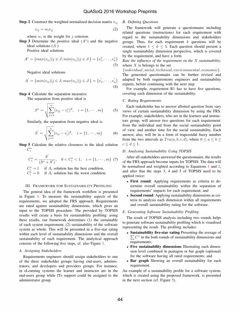
Step 2 Construct the weighted normalised decision matrix vij

vij = wirij (2)

where wi is the weight for j criterion.Step 3 Determine the positive ideal (A∗) and the negative

ideal solutions (A′):

Positive ideal solutions

A∗ = {max(vij)|j ∈ J ;min(vij)|j ∈ J′} = {v∗1 , · · · , v∗n}(3)

Negative ideal solutions

A′= {min(vij)|j ∈ J ;max(vij)|j ∈ J′} = {v

′

1, · · · , v′

n}(4)

Step 4 Calculate the separation measures:The separation from positive ideal is

S∗ =

√√√√ n∑j=1

(vij − v∗i )2, i = {1, · · · ,m} (5)

Similarly, the separation from negative ideal is

S′=

√√√√ n∑j=1

(vij − v′

i)2, i = {1, · · · ,m} (6)

Step 5 Calculate the relative closeness to the ideal solutionC∗i

C∗i =S

′

(S∗ + S′), 0 < C∗i < 1, i = {1, · · · ,m} (7)

C∗i = 1 if Ai solution has the best condition,C∗i = 0 if Ai solution has the worst condition.

III. FRAMEWORK FOR SUSTAINABILITY PROFILING

The general idea of the framework workflow is presentedin Figure 1. To measure the sustainability aspects of therequirements, we adopted the FRS approach. Requirementsare rated against sustainability dimensions, which gives aninput to the TOPSIS procedure. The provided by TOPSISresults will create a basis for sustainability profiling: usingthese results, our framework determines (1) the sustainableof each system requirement, (2) sustainability of the softwaresystem as whole. This will be presented in a five-star ratingwithin each level of sustainability dimensions and the overallsustainability of each requirement. The analytical approachconsists of the following five steps, cf. also Figure 1.

A. Assigning Stakeholders

Requirements engineers should assign stakeholders to oneof the three stakeholder groups having end-users, adminis-trators, and developers and providers groups. For instance,in eLearning systems the learner and instructor are in theend-users group while ITs support could be assigned to theadministrator group.

B. Defining Questions

The framework will generate a questionnaire includingrelated questions (instructions) for each requirement withregard to the sustainability dimensions and stakeholdersgroups. Thus, for each requirement k questions will becreated, where 1 ≤ k ≤ 5. Each question should present asingle sustainability dimension perspective, which is coveredby the requirement, and have a formRate the influence of the requirement on the X sustainability,where X is belongs to the set{individual, social, technical, environmental, economic}.The generated questionnaire can be further revised andadapted by both requirements engineers and sustainabilityexperts, before continuing with the next step.

For example, requirement R1 has to have five questions,covering each dimension of the sustainability.

C. Rating Requirements

Each stakeholder has to answer allotted question from varyviews of certain sustainability dimension by using the FRS.For example, stakeholders, who are in the learners and instruc-tors group, will answer two questions for each requirement:from the individual and from the social sustainability pointof view. and another time for the social sustainability. Eachanswer, also, will be in a form of trapezoidal fuzzy numberfrom the two intervals as Tra(a, b, c, d), where 0 ≤ a ≤ b ≤c ≤ d ≤ 1.

D. Analysing Sustainability Using TOPSIS

After all stakeholders answered the questionnaire, the resultsof the FRS approach become inputs for TOPSIS. The data willbe normalised and weighted according to Equations 1 and 2,and after that the steps 3, 4 and 5 of TOPSIS need to beapplied twice:• First round: Applying requirements as criteria to de-

termine overall sustainability within the separation ofrequirements’ impacts for each requirement; and

• Second round: Applying sustainability dimensions as cri-teria to analysis each dimension within all requirementsand overall sustainability rating for the software.

E. Generating Software Sustainability Profiling

The result of TOPSIS analysis including two rounds helpsto generate software sustainability profiling which is visualisedrepresenting the result. The profiling includes:• Sustainability five-star rating Presenting the average of∑

C∗ in the both rounds of sustainability dimensions andrequirements;

• Five sustainability dimensions Illustrating each dimen-sion level combined in pentagon or bar graph (optional)for the software having all rated requirements; and

• Bar graph Showing an overall sustainability for eachrequirement.

An example of a sustainability profile for a software system,which is created using the proposed framework, is presentedin the next section (cf. Figure 5).


44

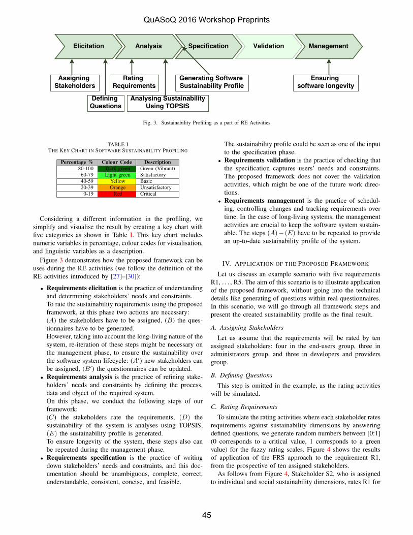
Fig. 3. Sustainability Profiling as a part of RE Activities

TABLE ITHE KEY CHART IN SOFTWARE SUSTAINABILITY PROFILING

Percentage % Colour Code Description80-100 Dark green Green (Vibrant)60-79 Light green Satisfactory40-59 Yellow Basic20-39 Orange Unsatisfactory

0-19 Red Critical

Considering a different information in the profiling, wesimplify and visualise the result by creating a key chart withfive categories as shown in Table I. This key chart includesnumeric variables in percentage, colour codes for visualisation,and linguistic variables as a description.

Figure 3 demonstrates how the proposed framework can beuses during the RE activities (we follow the definition of theRE activities introduced by [27]–[30]):

• Requirements elicitation is the practice of understandingand determining stakeholders’ needs and constraints.To rate the sustainability requirements using the proposedframework, at this phase two actions are necessary:(A) the stakeholders have to be assigned, (B) the ques-tionnaires have to be generated.However, taking into account the long-living nature of thesystem, re-iteration of these steps might be necessary onthe management phase, to ensure the sustainability overthe software system lifecycle: (A′) new stakeholders canbe assigned, (B′) the questionnaires can be updated.

• Requirements analysis is the practice of refining stake-holders’ needs and constraints by defining the process,data and object of the required system.On this phase, we conduct the following steps of ourframework:(C) the stakeholders rate the requirements, (D) thesustainability of the system is analyses using TOPSIS,(E) the sustainability profile is generated.To ensure longevity of the system, these steps also canbe repeated during the management phase.

• Requirements specification is the practice of writingdown stakeholders’ needs and constraints, and this doc-umentation should be unambiguous, complete, correct,understandable, consistent, concise, and feasible.

The sustainability profile could be seen as one of the inputto the specification phase.

• Requirements validation is the practice of checking thatthe specification captures users’ needs and constraints.The proposed framework does not cover the validationactivities, which might be one of the future work direc-tions.

• Requirements management is the practice of schedul-ing, controlling changes and tracking requirements overtime. In the case of long-living systems, the managementactivities are crucial to keep the software system sustain-able. The steps (A)− (E) have to be repeated to providean up-to-date sustainability profile of the system.

IV. APPLICATION OF THE PROPOSED FRAMEWORK

Let us discuss an example scenario with five requirementsR1, . . . , R5. The aim of this scenario is to illustrate applicationof the proposed framework, without going into the technicaldetails like generating of questions within real questionnaires.In this scenario, we will go through all framework steps andpresent the created sustainability profile as the final result.

A. Assigning Stakeholders

Let us assume that the requirements will be rated by tenassigned stakeholders: four in the end-users group, three inadministrators group, and three in developers and providersgroup.

B. Defining Questions

This step is omitted in the example, as the rating activitieswill be simulated.

C. Rating Requirements

To simulate the rating activities where each stakeholder ratesrequirements against sustainability dimensions by answeringdefined questions, we generate random numbers between [0:1](0 corresponds to a critical value, 1 corresponds to a greenvalue) for the fuzzy rating scales. Figure 4 shows the resultsof application of the FRS approach to the requirement R1,from the prospective of ten assigned stakeholders.

As follows from Figure 4, Stakeholder S2, who is assignedto individual and social sustainability dimensions, rates R1 for


45

.0 10 20 30 40 50 60 70 80 90 100

Green( Vibrant )

Critical

.0 10 20 30 40 50 60 70 80 90 100

Green( Vibrant )

Critical

S 2

.0 10 20 30 40 50 60 70 80 90 100

Green( Vibrant )

Critical

S 2

.0 10 20 30 40 50 60 70 80 90 100

Green( Vibrant )

Critical

S 1

.0 10 20 30 40 50 60 70 80 90 100

Green( Vibrant )

Critical

S 3

.0 10 20 30 40 50 60 70 80 90 100

Green( Vibrant )

Critical

S 3

.0 10 20 30 40 50 60 70 80 90 100

Green( Vibrant )

Critical

S 1

.0 10 20 30 40 50 60 70 80 90 100

Green( Vibrant )

Critical

S 4

.0 10 20 30 40 50 60 70 80 90 100

Green( Vibrant )

Critical

S 4

.0 10 20 30 40 50 60 70 80 90 100

Green( Vibrant )

Critical

S 5

.0 10 20 30 40 50 60 70 80 90 100

Green( Vibrant )

Critical

S 5

.0 10 20 30 40 50 60 70 80 90 100

Green( Vibrant )

Critical

S 5

.0 10 20 30 40 50 60 70 80 90 100

Green( Vibrant )

Critical

S 6

.0 10 20 30 40 50 60 70 80 90 100

Green( Vibrant )

Critical

S 6

.0 10 20 30 40 50 60 70 80 90 100

Green( Vibrant )

Critical

S 6

.0 10 20 30 40 50 60 70 80 90 100

Green( Vibrant )

Critical

S 7

.0 10 20 30 40 50 60 70 80 90 100

Green( Vibrant )

Critical

S 7

.0 10 20 30 40 50 60 70 80 90 100

Green( Vibrant )

Critical

S 7

.0 10 20 30 40 50 60 70 80 90 100

Green( Vibrant )

Critical

S 8

.0 10 20 30 40 50 60 70 80 90 100

Green( Vibrant )

Critical

S 8

.0 10 20 30 40 50 60 70 80 90 100

Green( Vibrant )

Critical

S 8

.0 10 20 30 40 50 60 70 80 90 100

Green( Vibrant )

Critical

S 9

.0 10 20 30 40 50 60 70 80 90 100

Green( Vibrant )

Critical

S 9

.0 10 20 30 40 50 60 70 80 90 100

Green( Vibrant )

Critical

S 9

.0 10 20 30 40 50 60 70 80 90 100

Green( Vibrant )

Critical

S 10

.0 10 20 30 40 50 60 70 80 90 100

Green( Vibrant )

Critical

S 10

.0 10 20 30 40 50 60 70 80 90 100

Green( Vibrant )

Critical

S 10

A Representative Rating

Social

Tech

nical

Econ

omic

Environ

men

t

Individu

alIndividu

al

Individu

al

Individu

al

Social

Social

Social

Social

Social

Social

Econ

omic

Environ

men

t

Tech

nical

Econ

omic

Environ

men

tEc

onom

icEn

viron

men

t

Tech

nical

Econ

omic

Econ

omic

Environ

men

tEn

viron

men

t

Fig. 4. Example of Fuzzy Rating Scale for Requirement (R1)

TABLE IIOUTPUT EXAMPLES OF FUZZY RATING SCALE FOR REQUIREMENTS ANALYSIS

Dimension S1 S2 S3 S4 S5 S6 S7 S8 S9 S10Individual 0.573 0.754 0.625 0.914Social 0.276 0.727 0.087 0.917 0.377 0.942 0.066Technical 0.579 0.808 0.324Economic 0.158 0.446 0.340 0.345 0.362 0.529

R1

Environment 0.382 0.351 0.799 0.291 0.986 0.130Individual 0.281 0.472 0.232 0.289Social 0.096 0.587 0.605 0.301 0.660 0.455 0.407Technical 0.925 0.677 0.309Economic 0.093 0.506 0.738 0.567 0.459 0.395

R2


R3


R4


R5

Environment 0.214 0.704 0.662 0.949 0.714 0.583

individual perspective as Tra(0.51, 0.66, 0.856, 1.00) whilesocial perspective as Tra(0.60, 0.66, 0.75, 0.9). We calculatefuzzy values from each fuzzy rating by mean measurement,so individual and social means of R1 for S2 are 0.754 and0.727, respectively.

D. Analysing Sustainability

In the next step, all the FRS outputs become inputs forTOPSIS, cf. Table II. These data are normalised according toEquation 1 for the five system requirements R1, . . . , R5 withinthe individual, social, technical, economic and environmentaldimensions of sustainability. The result of normalisation steppresented in Table III.

The weighted normalisation that was constructed accordingto Equation 2 is showed in Table IV. Following the TOPSISprocedure, we calculate for both rounds the separation mea-sures from positive ideal S∗ and negative ideal solutions S

′, as

well as the relative closeness C∗. The results are summarisedin Tables V and VI. Noteworthy, we could calculate thenegative impact of economic and environmental sustainabilitydimensions via the negative ideal solution that maximises thecost criteria and minimises the benefit criteria.

E. Sustainability Profiling

The generating software sustainability profiling is presentedin Figure 5 within an overall of 49% sustainability which is themean of

∑C∗ in the two rounds (in Table V and VI). Among


46

Eco

no

mic

Environmental T

ech

nic

al

SocialIn

dividual

Overall 10 30 50 70 90

Green (Vibrant)Green (Vibrant)

SatisfactorySatisfactory

BasicBasicUnsatisfactoryUnsatisfactory

CriticalCritical

80 – 100 %80 – 100 %

60 – 79 %60 – 79 %

40 – 59 %40 – 59 %

20 – 39 %20 – 39 %

0 – 19 %0 – 19 %

0 0 .2 0 .4 0 .6 0 .8

R 1

R 2

R 3

R 4

R 5

Fig. 5. Sustainability Profile of a Software System using the default colour schema. To increase accessibility of our approach, we also provide anothercolouring option for colour-challenged people. In this option the red colour is replaced by blue.

TABLE IIITHE NORMALISATION DECISION (STEP 1) USING EQUATION 1

Dimensions R1 R2 R3 R4 R5Individual 0.536 0.238 0.529 0.336 0.512

Social 0.462 0.423 0.425 0.498 0.422Technical 0.444 0.496 0.275 0.408 0.559Economic 0.421 0.533 0.304 0.562 0.358

Environment 0.431 0.414 0.431 0.374 0.561

TABLE IVTHE WEIGHTED NORMALISATION STEPS FROM EQUATION 2

Dimensions R1 R2 R3 R4 R5Individual 0.146 0.033 0.166 0.063 0.126

Social 0.085 0.081 0.084 0.108 0.067Technical 0.097 0.136 0.043 0.089 0.144Economic 0.058 0.105 0.035 0.113 0.040

Environment 0.081 0.084 0.094 0.066 0.128

TABLE VRESULTS OF THE STEPS 4 AND 5 IN THE FIRST ROUND

Dimensions S* S’ C*Individual 0.0917 0.130 0.586

Social 0.143 0.118 0.452Technical 0.134 0.137 0.505Economic 0.132 0.104 0.440

Environment 0.093 0.151 0.617

TABLE VIRESULTS OF THE STEPS 4 AND 5 IN THE SECOND ROUND

R1 R2 R3 R4 R5S* 0.116 0.139 0.135 0.191 0.121S’ 0.179 0.091 0.154 0.088 0.119C* 0.607 0.394 0.533 0.317 0.497

the five requirements, R1 meets the highest level as satisfactoryas well as environmental dimensions. Also, individual, social,technical and economic dimensions become basic as the lowestlevel of software sustainability including the five requirements

in this example.

V. DISCUSSION AND CONCLUSIONS

In this paper, we introduced a framework for software sus-tainability profiling. We also presented and example scenarioto provide a numerical illustration on how the framework canbe applied. The framework allows to create the followingprofiling elements:

1) Sustainability five-star rating for overall sustainabilityranking of entire software requirements;

2) Visualisation of the five sustainability dimensions as apentagon graph (and, optionally, also a bar graph) for alldimension levels of the entire software requirements; and

3) Bar graph for overall sustainability of each requirement.In our framework we apply a quantitative approach to

measure sustainability of the software systems. The fuzzyrating scale is utilised to overcome inexplicit choices in ques-tionnaires and increase the usability of the framework. TheTOPSIS approach for requirements analysis is used to analyseranking within the best ideal solution and the worst idealsolution among requirements that could assist to recognise thepositive and negative impacts on sustainability via maximisingor minimising the benefit or cost.

In the case of long-living systems, it is crucial to keep thesoftware system sustainable over the whole lifecycle of thesystem. The stakeholders requirements and preferences mightchange over the time the system is in use, and proposed frame-work allows to analyse the up-to-date system sustainabilityprofiles, based on system characteristics and the up-to-dateratings (quotations) of the corresponding requirements.

One of the core features of the framework is readabilityof the sustainability profiles, which also implies the usabilityof the proposed framework. For example, we apply the five-star rating to present sustainability ratings, as this rating isperceived as a common one in other areas: the five-star ratinghas become a standard for electricity consumption labellingin electronic appliances such as air conditioners and computer


47

monitors, allowing an energy efficient choice by reducingenergy use and emissions (i.e., to increase environmentalsustainability).

We follow the traffic lights colouring schema, where crit-ical values are marked red and green (vibrant) are markedgreen to increase readability and graphic visualisation. Thesecolours and their descriptions have been used in Green IT andSustainability Developments. To increase accessibility of ourapproach, we also provide another colouring option for colour-challenged people, where the red colour is replaced by blue.Finally, there are two options to present the five sustainabilitydimensions as a pentagon or bar graph because it might beargued that the pentagon graph could be harder to read andneed more effort to analyse represented data than the bargraph, so we provide the bar graph option for representingthe five sustainability dimensions.

Future work: The main direction of our future work onthe proposed framework is to develop a tool for softwaresustainability profiling, allowing to perform the frameworksteps within a single platform. We also would like to applythe proposed framework to our earlier work on the analysisof the RE aspects of ELearning systems [31] as well as ofgeographically distributed systems and within global productdevelopment [32]–[34].

ACKNOWLEDGEMENT

The first author is supported by a scholarship from UmmAl-Qura University, Saudi Arabia.

REFERENCES

[1] B. Penzenstadler, A. Raturi, D. Richardson, and B. Tomlinson, “Safety,security, now sustainability: The nonfunctional requirement for the 21stcentury,” Software, IEEE, vol. 31, no. 3, pp. 40–47, 2014.

[2] F. Berkhout and J. Hertin, “Impacts of information and communi-cation technologies on environmental sustainability: Speculations andevidence,” Report to the OECD, Brighton, vol. 21, 2001.

[3] P. Lago and T. Jansen, “Creating environmental awareness in service ori-ented software engineering,” in Service-Oriented Computing. Springer,2011, pp. 181–186.

[4] S. Naumann, M. Dick, E. Kern, and T. Johann, “The greensoft model: Areference model for green and sustainable software and its engineering,”Sustainable Computing: Informatics and Systems, vol. 1, no. 4, pp. 294–304, 2011.

[5] B. Penzenstadler and H. Femmer, “A generic model for sustainabilitywith process- and product-specific instances,” in Proceedings of the 2013Workshop on Green in/by Software Engineering, ser. GIBSE ’13. NewYork, NY, USA: ACM, 2013, pp. 3–8.

[6] G. G. Calienes, “Requirements prioritization framework for developinggreen and sustainable software using anp-based decision making,” 2013.

[7] B. Penzenstadler, “Infusing green: Requirements engineering for greenin and through software systems,” Christopher Arciniega, Birgit Penzen-stadler TechReport UCI-ISR-14-2 June, 2014.

[8] C. Becker, S. Betz, R. Chitchyan, L. Duboc, S. M. Easterbrook,B. Penzenstadler, N. Seyff, and C. C. Venters, “Requirements: The keyto sustainability,” IEEE Software, vol. 33, no. 1, pp. 56–65, Jan. 2016.

[9] V. G. Duffy, Improving Sustainability through Usability. Cham:Springer International Publishing, 2014, pp. 507–519.

[10] S. de la Rosa de Saa, M. A. Gil, G. Gonzalez-Rodrıguez, M. T. Lopez,and M. A. Lubiano, “Fuzzy rating scale-based questionnaires and theirstatistical analysis,” IEEE Transactions on Fuzzy Systems, vol. 23, no. 1,pp. 111–126, Feb 2015.

[11] M. Behzadian, S. K. Otaghsara, M. Yazdani, and J. Ignatius, “Astate-of the-art survey of TOPSIS applications,” Expert Systems withApplications, vol. 39, no. 17, pp. 13 051 – 13 069, 2012.

[12] D. Mairiza, D. Zowghi, and V. Gervasi, “Utilizing TOPSIS: A MultiCriteria Decision Analysis Technique for Non-Functional RequirementsConflicts,” in RE, ser. Communications in Computer and InformationScience, D. Zowghi and Z. Jin, Eds. Springer, 2014, vol. 432, pp.31–44.

[13] P. Achimugu, A. Selamat, R. Ibrahim, and M. N. Mahrin, “A system-atic literature review of software requirements prioritization research,”Information and Software Technology, vol. 56, no. 6, pp. 568 – 585,2014.

[14] E. Hull, K. Jackson, and J. Dick, Requirements engineering. SpringerScience & Business Media, 2010.

[15] G. Lami, F. Fabbrini, and M. Fusani, Software Sustainability froma Process-Centric Perspective, ser. Communications in Computer andInformation Science. Springer Berlin Heidelberg, 2012, vol. 301, ch.Systems, Software and Services Process Improvement, pp. 97–108.

[16] B. Penzenstadler, Green in Software Engineering. Cham: SpringerInternational Publishing, 2015, ch. From Requirements Engineering toGreen Requirements Engineering, pp. 157–186.

[17] R. Goodland, “Sustainability: human, social, economic and environmen-tal,” Encyclopedia of Global Environmental Change. John Wiley & Sons,2002.

[18] M. Razavian, G. Procaccianti, D. A. Tamburri et al., “Four-dimensionalsustainable e-services,” EnviroInfo, Sep, 2014.

[19] P. James, Urban sustainability in theory and practice: circles of sustain-ability. Routledge, 2014.

[20] B. Stewart and A. Khare, “elearning and the sustainable campus,” inTransformative Approaches to Sustainable Development at Universities.Springer, 2015, pp. 291–305.

[21] D. Gmach, Y. Chen, A. Shah, J. Rolia, C. Bash, T. Christian, andR. Sharma, “Profiling sustainability of data centers,” in Proceedings ofthe 2010 IEEE International Symposium on Sustainable Systems andTechnology, May 2010, pp. 1–6.

[22] E. A. Jagroep, J. M. van der Werf, S. Brinkkemper, G. Procaccianti,P. Lago, L. Blom, and R. van Vliet, “Software energy profiling:Comparing releases of a software product,” in Proceedings of the38th International Conference on Software Engineering Companion, ser.ICSE ’16. New York, NY, USA: ACM, 2016, pp. 523–532.

[23] T. Tullis and B. Albert, Measuring the User Experience, 2nd ed., ser.Interactive Technologies. Boston: Morgan Kaufmann, 2013.

[24] J. Horkoff and E. Yu, “Analyzing goal models: Different approachesand how to choose among them,” in Proceedings of the 2011 ACMSymposium on Applied Computing, ser. SAC ’11. New York, NY,USA: ACM, 2011, pp. 675–682.

[25] M. A. Lubiano, S. de la Rosa de Sa, M. Montenegro, B. Sinova, andM. ngeles Gil, “Descriptive analysis of responses to items in question-naires. why not using a fuzzy rating scale?” Information Sciences, vol.360, pp. 131 – 148, 2016.

[26] J. R. S. C. Mateo, TOPSIS. London: Springer London, 2012, pp. 43–48.

[27] R. H. Thayer and M. Dorfman, Software Requirements Engineering.Wiley-IEEE Press, 2000, ch. Introductions, Issues, and Terminology,pp. 3–40.

[28] B. Nuseibeh and S. Easterbrook, “Requirements engineering: Aroadmap,” in Proceedings of the Conference on The Future of SoftwareEngineering, ser. ICSE ’00. New York, NY, USA: ACM, 2000, pp.35–46.

[29] P. Sawyer, I. Sommerville, and S. Viller, “Requirements process im-provement through the phased introduction of good practice,” SoftwareProcess: Improvement and Practice, vol. 3, no. 1, pp. 19–34, 1997.

[30] I. Sommerville, Software Engineering, 9th ed. USA: Addison-WesleyPublishing Company, 2010.

[31] A. D. Alharthi, M. Spichkova, and M. Hamilton, “Requirements en-gineering aspects of elearning systems,” in Proceedings of the ASWEC2015 24th Australasian Software Engineering Conference. ACM, 2015,pp. 132–133.

[32] M. Spichkova and H. Schmidt, “Requirements engineering aspects ofa geographically distributed architecture,” in 10th International Con-ference on Evaluation of Novel Approaches to Software Engineering(ENASE 2015), 2015.

[33] M. Spichkova, H. W. Schmidt, M. R. I. Nekvi, and N. H. Madhavji,“Structuring diverse regulatory requirements for global product develop-ment,” in Requirements Engineering and Law. IEEE, 2015, pp. 57–60.

[34] M. Spichkova, H. Liu, and H. Schmidt, “Towards quality-orientedarchitecture: Integration in a global context,” in European Conference

on Software Architecture Workshops. ACM, 2015, p. 64.


48

Improving Recall in Code Search by IndexingSimilar Codes under Proper Terms

Abdus Satter∗ and Kazi Sakib†Institute of Information Technology, University of Dhaka, Dhaka, Bangladesh

Email: ∗[email protected], †[email protected]

Abstract—The recall of a code search engine is reduced,if feature-wise similar code fragments are not indexed undercommon terms. In this paper, a technique named Similarity BasedMethod Finder (SBMF) is proposed to alleviate this problem. Thetechnique extracts all the methods from a source code corpus andconverts these into reusable methods (i.e., program slice) throughresolving data dependency. Later, it finds similar methods bychecking signature (i.e., input and output types) and executingmethods for a randomly generated set of input values. Methodsare considered as feature-wise similar if these produce the sameoutput set. In order to index these methods against common andproper terms, SBMF selects the terms that are found in mostof the methods. Finally, query expansion is performed beforesearching the index to solve the vocabulary mismatch problem. Inorder to evaluate SBMF, fifty open source projects implementingnine different functionalities or features were used. The resultswere compared with two types of techniques - Keyword BasedCode Search (KBCS) and Interface Driven Code Search (IDCS).On an average, SBMF retrieves 38% and 58% more relevantmethods than KBCS and IDCS, respectively. Moreover, it issuccessful for all the features by retrieving at least one relevantmethod representing each feature whereas IDCS and KBCS aresuccessful for 3 and 7 features out of 9 respectively.

Index Terms—code search, code reuse, method search

I. INTRODUCTION

The recall of a code search engine, indicated by the numberof relevant codes that is retrieved from the code repository,usually depends on the indexing mechanism and query for-mulation techniques. Proper indexing and query understandinghelp to retrieve relevant code snippets that satisfy user needs[1]. Most of the code search engines employ InformationRetrieval (IR) centric approaches for indexing source code[2]. The working principle behind these approaches is toconstruct a term-based index, by extracting keywords fromsource codes. A common problem of these approaches isthat a pair of codes - having same functionality, but writtenusing different keywords are indexed against different terms.A traditional code search engine misses some important codefragments, because of this keyword matching policy. It resultsin a low recall code search engine with poor performance onbenchmark datasets [3].

To improve recall of a code search engine, similar codefragments should be indexed under the same terms. However,it is challenging to automatically and efficiently determinethat two code fragments are identical or similar [4]. Althoughidentical code fragments can be detected through keywordsmatching [5], detecting feature wise similar code blocks is

difficult. The reason is that automatically perceiving the intentof a code block is still a research challenge [6]. Another chal-lenge is to select proper terms that best represent similar codefragments. For example, assume that there are two methodsthat perform bubble sort - “x” and “sort”. Here, between twoterms, “sort” is semantically more relevant name than “x”. Itis a challenging task to automatically determine that “sort” isthe better keyword to represent these methods. Again, a codefragment may contain terms, which are not useful to expressits intent (i.e., implemented feature) properly. Indexing basedon these keywords reduces matching probability between userquery and these keywords. It happens because, user querydefines functionality but the extracted keywords do not expressthe feature properly. So, instead of using these keywords, moremeaningful terms need to be selected that best match the query.

Researchers have proposed various techniques to improvethe performance of code search engines where recall is con-sidered as one of the performance indicators. These techniquescan be broadly classified into four types like Keyword BasedCode Search (KBCS), Interface Driven Code Search (IDCS),Test Driven Code Search (TDCS), and Semantic Based CodeSearch (SBCS). In KBCS [2], [7], [8], [9], [10], source codesare indexed based on the terms generated from the code andsearching is performed on the index. As this approach doesnot consider similarity between source codes having differentkeywords, it cannot retrieve more relevant codes. In order todefine required component interface as query, and find relevantcomponents, IDCS [11], [12], [13] was proposed. It is possibleto have two or more code fragments that contain differentinterfaces but perform the same task. IDCS considers thatthese code fragments are different due to having differentinterfaces. Thus, it does not retrieve these all together. Toautomatically find and adapt reusable components, TDCS [14],[15] and SBCS [16], [17] were proposed. These are effective interms of precision as test cases are employed on the retrievedcodes. In these approaches, most of the test cases fail not onlyfor functional requirements mismatch but also for syntacticmismatch of the interface definition [15]. For this reason,semantically relevant code fragments cannot be retrieved andthe recall is decreased.

In this paper a technique named Similarity Based MethodFinder (SBMF) is proposed to retrieve more relevant methodsfrom code base. The technique first parses all the methodsfrom the source code to construct a repository of methods.It generates data dependency graph for each method and


49

converts the method into reusable method (i.e., program slice)through resolving data dependency, and redefining parametersand return type. Later, all the methods are clustered into anumber of clusters where methods in the same cluster performthe same task. To detect feature-wise similarity among a setof methods’ signatures (i.e., parameters and return types) ofthese methods are checked. Methods having the same signatureare then executed against a set of randomly generated inputvalues. Among these methods, those which produce the sameoutput are considered as feature-wise similar and a cluster isconstructed to store these methods. To identify proper termsfor a cluster, keywords are obtained from the methods in thecluster and method frequency is calculated for each term.Such terms are considered as representative terms if theseare found in most of the methods of the cluster. All themethods of the cluster are then indexed against the terms sothat these are retrieved all together if a query term matchesone of these methods. At last, user query is expanded byadding synonyms of each query term to increase the matchingprobability between the query terms and index terms [7].

In order to evaluate the proposed technique, a tool wasdeveloped. Two types of code search techniques, KBCS andIDCS, were compared with SBMF to show its efficiency.An existing system named Sourcerer [8] was used for theimplementation of KBCS and IDCS. However, SBCS andTDCS were not considered for comparison, because thesewere proposed to improve precision rather than recall. Forcomparative result analysis, three metrics were used whichare recall, number of methods retrieved and feature successful-ness. Here, feature successfulness determines whether at leastone relevant method is retrieved or not against user queriesprovided for a feature. In the context of this paper, A featurecan be considered as a requirement given to a developer toimplement. 50 open source projects were selected to carry outthe experiment. The result analysis shows that on an averageSBMF increases recall by 38% and 58% more than KBCSand IDCS, respectively against 170 queries. Besides, SBMFis successful for all the features whereas KBCS and IDCS aresuccessful for 7 and 3 features out of 9 respectively.

II. RELATED WORKS

Reusing existing code fragments reduces development timeand effort [18]. For this reason, searching for reusable codesnippets has become a common task among the developersduring software development [19]. Various techniques havebeen proposed in the literature to improve the performanceof code search engine in terms of recall, precision, querysuccessfulness, etc. These techniques can be broadly classifiedinto four categories which are Keyword Based Code Search(KBCS), Interface Driven Code Search (IDCS), SemanticBased Code Search (SBCS), and Test Driven Code Search(TDCS). Significant works related to each category are dis-cussed in the following subsections.

A. Keyword based Code Search (KBCS)

In KBCS, source code is considered as plain text documentwhere traditional IR centric approaches are employed to in-dex the code and query over the index [20]. Besides, othermetadata such as comments, file name, commit message, etc.are used to retrieve relevant code fragments from a repositoryof source codes. One of the techniques related to KBCSis JSearch which indexes source code against the keywordsextracted from the code [2]. However, it cannot retrieve allthe code snippets that implement the same feature but containdifferent keywords. This is because, it does not check feature-wise similarity to detect common terms for these fragments.

Several techniques like Sourcerer [8], Codifier [9], krugle[10], etc. were proposed to provide infrastructure for largescale code search. These techniques use both structural andsemantic information of source code to construct index. Struc-tural information comprises language, source file, related doc-uments, classes, methods, dependencies, and so on. Semanticinformation of a program is gathered by generating termsfrom method name, class name, field name, comments, etc.Although these techniques adopt both types of informationto fetch more relevant code fragments, these cannot retrievefeature-wise similar code blocks simultaneously. The reasonis that all these information are stored following IR basedindexing mechanism, and no checking is performed to indexsimilar code snippets under common proper terms.

B. Semantic Based Code Search (SBCS)

As open source codes are increasing day by day, it is thoughtthat a significant amount of code that is written today, hasalready been available in the internet. However, reusing theseexisting codes often does not directly meet user needs orrequires modifications. In order to find existing codes thatsupport user requirements, a technique in form of SBCS wasproposed by Steven [16]. It takes keywords that represent userrequirements, and retrieves relevant code fragments containingthese keywords. Later, it runs user provided test cases onthe fetched code snippets and passed codes are delivered asfinal search result. It performs well in terms of precision butrecall is reduced since proper terms are not determined whileindexing feature-wise similar codes. So, some semanticallysimilar code fragments cannot be fetched due to indexing theseunder inappropriate terms.

Sometimes, developers need to convert one type of ob-ject to another. To get example code implementing suchconversion, Niyana proposed a technique named XSnippet[17]. It creates graph from source code by adopting codemining algorithm. The graph represents data flow within thecorresponding source code. Moreover, user query is definedby providing input type and output type. For a user query,all the generated graphs are searched to find those codefragments that convert the input type into the output type.In this technique. developers need to provide exact input typeand output type for getting example code blocks. Otherwise,it cannot retrieve code fragments that may satisfy user needs.However, according to the searching behavior, developers are


50

more interested in using keywords rather than concrete datatypes to define their query [21].

C. Test Driven Code Search (TDCS)

TDCS is a special type of SBCS where test cases areused to obtain program semantics. Lemos et al. proposed aTDCS technique named CodeGenie to support method levelsearching [14]. The technique takes method signature as queryfrom the test cases written by developers. It uses Sourcererinfrastructure to retrieve relevant functions against the query.Next, all the test cases are executed for each retrieved method.Resultant methods are ranked based on the number of testcases successfully passed. Although the technique increasesprecision, it produces low recall. The reason is that it per-forms keyword matching to fetch methods from index withoutjustifying the appropriateness of the keywords.

Usually retrieved methods may not pass correspondingtest cases due to different order of the parameters, returntype or parameter type. To resolve these issues, Janjic et al.proposed a technique that refactors the code to adapt with theprogram context [15]. It applies every possible adaptations likereordering parameters, using super type or sub class type ofa given return or parameter type, converting primitive type toreference type, etc. Thus, it improves TDCS by finding morerelevant methods. However, it produces low recall because itdoes not index similar methods under common terms.

D. Inreface Driven Code Search (IDCS)

IDCS helps the developers to define their queries in a morestructured form rather than just a set of keywords joined byboolean expression. Signature matching was the first proposedIDCS technique to find relevant functions within a softwarelibrary [13]. The approach crawls all the methods in the library,and uses signature of each method for indexing. Other codesearch techniques such as Sourcecer, ParseWeb, and Strath-cona also support IDCS to improve the performance in codesearch [7]. Although IDCS assists to formulate user query,it does not select appropriate terms during indexing similarcodes that perform the same functionality. Thus, functionallyrelated code fragments will not be retrieved all together sincethese are indexed against inappropriate terms.

In order to find reusable code fragments, four types oftechniques have been proposed in the literature which areKBCS, IDCS, TDCS, and SBCS. All these techniques extractkeywords from source code to generate terms, and index cor-responding code against the terms. However, none of the tech-niques checks the appropriateness of the terms with respect toimplemented feature. As a result, the number of relevant codesretrieved is reduced due to indexing against improper term.Moreover, if two or more code snippets implement similarfeature but contain different terms, existing techniques cannotretrieve all these code fragments simultaneously. The reason isthat these are indexed against different terms. So, to improverecall in code search, feature-wise similar codes should beindexed under common appropriate terms.

III. PROPOSED TECHNIQUE

In this paper, a technique named Similarity based MethodFinder (SBMF) has been proposed to improve recall incode search. The technique comprises several steps such asReusable Method Generation, Clustering Similar Methods,Proper Term Selection, Handling Methods Having API/LibraryFunction call, Index Construction, and Query Expansion. Eachof the steps is discussed as follows.

A. Reusable Method Generation

In this step, the proposed technique first parses the sourcecode to identify all the methods in the code. For each method,it checks whether the body of that method contains any API/-function call statement or not. If no such statement is found,the technique takes the method to convert it into reusablemethod (i.e., program slice that can execute independentlywithout having any dependency on other methods). Later, adata dependency graph is constructed for the correspondingmethod to determine its input and output types. Although thesignature of the method expresses the input and output types,this is not sufficient enough to convert into reusable functionfor several scenarios. For example, a method may have returntype void but it may manipulate one or more variables thatare declared outside the body of the method. A method maynot have any parameter (i.e., void) but use variables that aredefined outside the body of the method. Again, the signatureof a method may explicitly state the input and output typesbut some variables may be used or manipulated by it andthese are declared outside the method body. Considering allof these scenarios, the technique generates data dependencygraph to redefine the signature and convert into reusablemethod. Each node in the graph denotes the variable and anedge from a to b (a → b) denotes variable a depends onvariable b. After constructing the graph, nodes that have indegree zero and variables denoted by these nodes are declaredoutside the method body, are considered as input parameters.Besides, nodes that have out degree zero are considered asoutput variables of the method. If multiple output nodes arefound, a complex data type is created where each field ofthe type denotes each node. The reason is that a methodreturn type can be a single data type - either primitive orcomplex data type. The technique uses the variables found inthe nodes containing in degree zero to generate parameters ofthe method. If a single node is found which out degree is zero,the type of the variable denoted by the node is used as returntype of the method. Otherwise, generated composite data typeas discussed earlier is used. The signature of the method isredefined by combining the return type, method name, andparameters. It is possible to have one or more variables thatare declared outside the method body. In the data dependencygraph, nodes representing these variables may have at leastone in degree and one out degree. In this case, the techniqueparses the source code and checks the declaration statementsof the variables to determine the types of the variables. Usingthis information, it adds declaration statement for each of thevariables at the beginning of the function body. Thus, the


51

technique makes the method self-executable without havingany external data dependency.

B. Clustering Similar Methods

To improve code search, it is required to check the similarityamong methods found in the code base. Two or more methodsmay perform the same task in different ways. So, feature-wisesimilar methods needs to be detected to retrieve the similarmethods all together. In Algorithm 1, the procedure namedClusterSimilarMethods takes a list of reusable methods(M ) as input which is constructed following the previous step.A variable C is declared to store different clusters of similarmethods where each cluster contains the methods that performthe same functionality (Algorithm 1 Line 2). A for loop isdeclared that iterates on M to construct cluster of similarmethods. The procedure IsInAnyCluster is invoked to checkwhether each method m (belongs to M ) is added to any clusteror not previously (Algorithm 1 Lines 4-5). If m does notbelong to any cluster, a variable cl is declared to contain all themethods similar to m. A set of input data is generated basedon the type of parameters found in the signature of m andcorresponding output is generated by executing m (Algorithm1 Lines 9-10). Here inputset and outputset determine theintent of m. Another for loop is declared to identify othermethods that are similar to m. In each iteration, the signatureof each method m′ (in M ) is matched with the signature ofm to check whether the input data set can be fed into themethod and return type is identical to m (Algorithm 1 Line15). If the signatures of both methods are identical, the methodm′ is executed for inputset and generated output is stored tooutputset′. If outputset and outputset′ are found the same,m′ is considered similar to m as both methods produce sameoutput for the same input data set (Algorithm 1 Lines 17-19).m′ is then added to cl to store all the methods similar to m.At last, cl is inserted to the list of all identified clusters (C).

C. Proper Term Selection

In order to retrieve more relevant methods, it is required toidentify proper terms for each method before indexing. Whentwo or more methods have different names or signatures, butimplement the same functionality, these methods should beindexed under common appropriate terms. As a result, all thesemethods will be obtained against user query. So, after gettingall the clusters from the previous step, representative termsare selected for each cluster. For a cluster, terms are obtainedfrom the methods found in the cluster through extracting,tokenizing, and stemming keywords found in the methods.Terms that are found in most of the methods are consideredas final representative terms for each of these methods.

D. Handling Methods Having API/Library Function call

As developers also search for example code to understandthe usage of an API, in this step, methods that have API callstatements are gathered. For each identified method, terms aregenerated from API call statements to index against the terms.As a result, if a query term does not match with the signature

Algorithm 1 Cluster Similar MethodsRequire: A list of methods (M ) for which search index will

be constructed1: procedure CLUSTERSIMILARMETHODS(M )2: C = ∅;3: for each m ∈ M do4: if IsInAnyCluster(m,C) == true then5: continue6: end if7: cl = ∅8: cl.add(m)9: inputset = generate a set of input data randomly

for m10: outputset = execute m and generate correspond-

ing output for inputset11: for each m′ ∈ M do12: if IsInAnyCluster(m′, C) == true then13: continue14: end if15: if m′.paramtersTypes ==

m.parametersTypes & m′.returnType =m.returnType then

16: outputset′ = execute m′ and generate cor-responding output for inputset

17: if outputset == outputset′ then18: cl.add(m′)19: end if20: end if21: end for22: C.add(cl)23: end for24: end procedure25: procedure ISINANYCLUSTER(m,C)26: found = false27: for c ∈ C do28: if m ∈ c then29: found = true30: break;31: end if32: end for33: return found34: end procedure

of a method but matches with the API invocation statements,the method is retrieved as API usage example code.

E. Index Construction and Query Expansion

After generating appropriate terms for each method andmerging similar ones, an index is built for searching desiredmethods. A posting list is created to construct index, whichmaps terms with corresponding methods. Later, user query isexpanded to retrieve more relevant methods against the query.

Two procedures named ConstructIndex and Query, arepresented in Algorithm 2 to build index of methods obtainedfrom the previous steps, and refine user query, respectively. To


52

construct the index, an empty posting list is declared, whichmaps each term to corresponding methods (Algorithm 2 Lines2). A nested for loop is defined, where the outer loop iterateson a list of methods (M ) given as input to the procedure(Algorithm 2 Lines 3-4). The inner loop iterates to get all theterms of each method in M . In addition, each term is checkedwhether the posting list contains it or not to add a new term inthe list (Algorithm 2 Lines 5-7). Next, the method is added tothe posting list against the term so that, when a query term willmatch with the term, the method will be retrieved (Algorithm2 Lines 8). After adding all the methods, the list is returnedby the procedure (Algorithm 2 Lines 11).

In procedure Query, a boolean query is given as an argu-ment, from which terms are separated and stored in a variablenamed queryTerms to expand the query (Algorithm 2, Lines13-14). A nested for loop is defined, where the outer loopiterates on these terms (Algorithm 2, Lines 15-17). In eachiteration, a temporary variable (expandedTerm) initializedwith the corresponding term, is used to store synonyms ofthe term. To expand each term, synonyms are appendedto expandedTerm in the inner loop (Algorithm 2, Lines17-19). Later, each term in queryTerms is replaced withcorresponding expandedTerm for the expansion of the query(Algorithm 2, Lines 20). As a result of the expansion, theprobability of matching a query string with the terms definedin the index increases. Finally, the query is executed in theindex to retrieve intended methods, which are returned by theprocedure (Algorithm 2, Lines 22-23).

IV. IMPLEMENTATION AND RESULT ANALYSIS

In order to perform comparative result analysis, the pro-posed technique (SBMF) was implemented in form of asoftware tool. 50 open source projects were selected as datasources for the experimental analysis. To evaluate the proposedtechnique, 170 queries representing 9 different features wereexecuted by the tool. For comparative analysis, same querieswere also run on Sourcerer that supports KBCS and IDCS.

A. Environmental Setup

This section outlines the softwares and frameworks requiredfor the experimental analysis. SBMF was implemented usingC# programming language. Moreover, some other tools werealso used, which are addressed as follows:• JavaParser: An open source library used to parse Java

source code (https://github.com/javaparser)• Apache Lucene: A popular search engine infrastructure

used to index java methods and query over the index(https://lucene.apache.org/)

• Luke: Open source lucene client used to execute queryon the lucene index and visualize the search results(https://github.com/DmitryKey)

B. Dataset Selection

In order to perform experimental analysis, 50 open sourceprojects from sourceforge (https://sourceforge.net/) were se-lected. Fraser and Arcuri showed that these projects are

Algorithm 2 Index Construction and Query ExpansionRequire: A list of methods (M ) containing signature, body

and terms of each method1: procedure CONSTRUCTINDEX(M )2: Map < String, List < Method >> postingList3: for each m ∈ M do4: for each t ∈ m.terms do5: if !postingList.keys.contains(t) then6: postingList.keys.add(t)7: end if8: postingList[t].add(m)9: end for

10: end for11: return postingList12: end procedure13: procedure QUERY(booleanQueryStr)14: queryTerms=get all terms from booleanQueryStr15: for each qt ∈ queryTerms do16: expandedTerm = qt17: for each syn ∈ synonyms of qt do18: expandedTerms+ =” OR ”+syn19: end for20: queryTerms.replace(qt, expandedTerm)21: end for22: methods = obtain method from the index satisfying

queryTerms23: return methods24: end procedure

statistically sound and representatives of open source projects[22].

A set of features were selected from the existing worksin code search [7], [16], [23], [24] as shown in Table I. Onthe other hand, to evaluate the proposed technique, a set ofqueries is selected from [7]. Here, each query is related to aparticular functionality shown in Table I and all the queriesare created randomly. 15 subjects were employed to identifyrelevant methods for the functionalities. Among 15 subjects,5 of them were senior Java developers and rest 10 weremasters student. The reason of choosing students in this studyis that they can play important role in software engineeringexperiments [25]. All the experimental datasets are availablein this link1.

C. Comparative Result Analysis

For comparative result analysis, SBMF was run on theexperimental datasets and the relevance of retrieved methodswere checked for each user query. Moreover, Sourcerer whichsupports KBCS and IDCS, was also run on the same datasetsand search results obtained by this were compared to SBMF.Three metrics were used to evaluate the performance of SBMFin comparison with KBCS and IDCS. These were recall, num-ber of retrieved methods, and feature successfulness. Detailed

1http://tinyurl.com/zdqmoqz


53

TABLE ISELECTED FUNCTIONALITIES WITH FREQUENCY

# Functionality # methods # queries1 decoding String 13 202 encrypting password 3 273 decoding a URL 3 214 generating MD5 hash 3 165 rotating array 2 256 resizing image 3 257 scaling Image 3 198 encoding string to html 2 69 joining string 47 36

result analysis with respect to each of the metrics is discussedas follows.

Recall Analysis: Recall is one of the most commonly usedmetrics to measure the performance of traditional IR system.As the intent of the paper is to improve recall in code search, itis considered as an important metric to evaluate the proposedtechnique. In this experiment, recall is defined as follows.

recall =number of retrieved relevant methods

number of relevant methods in the repository

Fig. 1 depicts a comparative recall analysis among SBMF,KBCS, and IDCS where X axis denotes the feature no. asshown in TABLE I and Y axis represents the measuredrecall. For feature 1 (Decoding String), approximately 15%recall is shown in Fig. 1 for both KBCS and IDCS whereas100% recall is found for SBMF. There are 13 methods inthe repository that implement the feature. Among these, twomethods are found which contain keywords decode and stringin method name and parameter respectively. As a result, thesemethods are retrieved by both KBCS and IDCS. However,these techniques cannot retrieve other 11 methods becausesignatures of these methods do not contain any term related todecode. While analyzing the source code of these methods, itis seen that the bodies of these methods use third party APIslike URLDecoder.decode(String, String), Hex.decode(String),Base64.decode(base64), etc. to implement the feature. SMBFtakes terms from API call statements and indexes against theterms to provide example codes regarding API usage. So, itretrieves all these 13 methods.

For feature 2 (Encrypting Password), IDCS cannot find anymethods but 66.67% and 33.3% relevant methods are retrievedby SBMF and KBCS respectively as shown in Fig. 1. To getthe methods that implement this feature, the following queryis provided to IDCS.

name:(encrypt) AND return:(String) AND parameter:(String)

Although there is a single method found in the code base thathas encrypt keyword in its name but does not have String inits parameter. So, IDCS cannot obtain this method but KBCSretrieves because query keyword matches with the methodname. However, SBMF retrieves one more method havingsignature crypt(String strpw,String strsalt). The reason is thatencrypt and crypt both express the same intent as detected bythe query expansion part of SBMF (Algorithm 2).

Fig. 1. Recall Analysis

Fig. 2. Number of Retrieved Methods

There are 3 relevant methods in the experimental projectsthat implement feature no. 3 (Decoding a URL). According toFig. 1 only a single method is retrieved by SBMF that producesrecall 33.33%. On the contrary, KBCS and IDCS cannotretrieve any method related to the feature. This is becauseno method contains decode and URL simultaneously in thesignature. Although one of these methods named getPath doesnot provide any semantic information representing the fea-ture, it invokes a library method - URLDecoder.decode(path,”UTF-8”) which implements the feature. SBMF considers theinvocation statement for getting more relevant terms and thus,retrieves this method. Two other methods cannot be retrievedby SBMF due to finding no structural similarity among theseand no keywords representing the feature.

According to Fig. 1, 100% recall is obtained for SBMF,and 33.33% for KBCS and IDCS individually with respect tofeature no. 4 (Generating MD5 hash). It is clear that SBMF

Fig. 3. Feature Successfulness Analysis


54

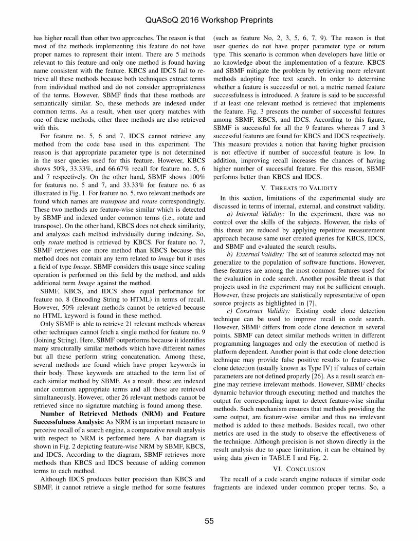
has higher recall than other two approaches. The reason is thatmost of the methods implementing this feature do not haveproper names to represent their intent. There are 5 methodsrelevant to this feature and only one method is found havingname consistent with the feature. KBCS and IDCS fail to re-trieve all these methods because both techniques extract termsfrom individual method and do not consider appropriatenessof the terms. However, SBMF finds that these methods aresemantically similar. So, these methods are indexed undercommon terms. As a result, when user query matches withone of these methods, other three methods are also retrievedwith this.

For feature no. 5, 6 and 7, IDCS cannot retrieve anymethod from the code base used in this experiment. Thereason is that appropriate parameter type is not determinedin the user queries used for this feature. However, KBCSshows 50%, 33.33%, and 66.67% recall for feature no. 5, 6and 7 respectively. On the other hand, SBMF shows 100%for features no. 5 and 7, and 33.33% for feature no. 6 asillustrated in Fig. 1. For feature no. 5, two relevant methods arefound which names are transpose and rotate correspondingly.These two methods are feature-wise similar which is detectedby SBMF and indexed under common terms (i.e., rotate andtranspose). On the other hand, KBCS does not check similarity,and analyzes each method individually during indexing. So,only rotate method is retrieved by KBCS. For feature no. 7,SBMF retrieves one more method than KBCS because thismethod does not contain any term related to image but it usesa field of type Image. SBMF considers this usage since scalingoperation is performed on this field by the method, and addsadditional term Image against the method.

SBMF, KBCS, and IDCS show equal performance forfeature no. 8 (Encoding String to HTML) in terms of recall.However, 50% relevant methods cannot be retrieved becauseno HTML keyword is found in these method.

Only SBMF is able to retrieve 21 relevant methods whereasother techniques cannot fetch a single method for feature no. 9(Joining String). Here, SBMF outperforms because it identifiesmany structurally similar methods which have different namesbut all these perform string concatenation. Among these,several methods are found which have proper keywords intheir body. These keywords are attached to the term list ofeach similar method by SBMF. As a result, these are indexedunder common appropriate terms and all these are retrievedsimultaneously. However, other 26 relevant methods cannot beretrieved since no signature matching is found among these.

Number of Retrieved Methods (NRM) and FeatureSuccessfulness Analysis: As NRM is an important measure toperceive recall of a search engine, a comparative result analysiswith respect to NRM is performed here. A bar diagram isshown in Fig. 2 depicting feature-wise NRM by SBMF, KBCS,and IDCS. According to the diagram, SBMF retrieves moremethods than KBCS and IDCS because of adding commonterms to each method.

Although IDCS produces better precision than KBCS andSBMF, it cannot retrieve a single method for some features

(such as feature No, 2, 3, 5, 6, 7, 9). The reason is thatuser queries do not have proper parameter type or returntype. This scenario is common when developers have little orno knowledge about the implementation of a feature. KBCSand SBMF mitigate the problem by retrieving more relevantmethods adopting free text search. In order to determinewhether a feature is successful or not, a metric named featuresuccessfulness is introduced. A feature is said to be successfulif at least one relevant method is retrieved that implementsthe feature. Fig. 3 presents the number of successful featuresamong SBMF, KBCS, and IDCS. According to this figure,SBMF is successful for all the 9 features whereas 7 and 3successful features are found for KBCS and IDCS respectively.This measure provides a notion that having higher precisionis not effective if number of successful feature is low. Inaddition, improving recall increases the chances of havinghigher number of successful feature. For this reason, SBMFperforms better than KBCS and IDCS.

V. THREATS TO VALIDITY

In this section, limitations of the experimental study arediscussed in terms of internal, external, and construct validity.

a) Internal Validity: In the experiment, there was nocontrol over the skills of the subjects. However, the risks ofthis threat are reduced by applying repetitive measurementapproach because same user created queries for KBCS, IDCS,and SBMF and evaluated the search results.

b) External Validity: The set of features selected may notgeneralize to the population of software functions. However,these features are among the most common features used forthe evaluation in code search. Another possible threat is thatprojects used in the experiment may not be sufficient enough.However, these projects are statistically representative of opensource projects as highlighted in [7].

c) Construct Validity: Existing code clone detectiontechnique can be used to improve recall in code search.However, SBMF differs from code clone detection in severalpoints. SBMF can detect similar methods written in differentprogramming languages and only the execution of method isplatform dependent. Another point is that code clone detectiontechnique may provide false positive results to feature-wiseclone detection (usually known as Type IV) if values of certainparameters are not defined properly [26]. As a result search en-gine may retrieve irrelevant methods. However, SBMF checksdynamic behavior through executing method and matches theoutput for corresponding input to detect feature-wise similarmethods. Such mechanism ensures that methods providing thesame output, are feature-wise similar and thus no irrelevantmethod is added to these methods. Besides recall, two othermetrics are used in the study to observe the effectiveness ofthe technique. Although precision is not shown directly in theresult analysis due to space limitation, it can be obtained byusing data given in TABLE I and Fig. 2.

VI. CONCLUSION

The recall of a code search engine reduces if similar codefragments are indexed under common proper terms. So, a


55

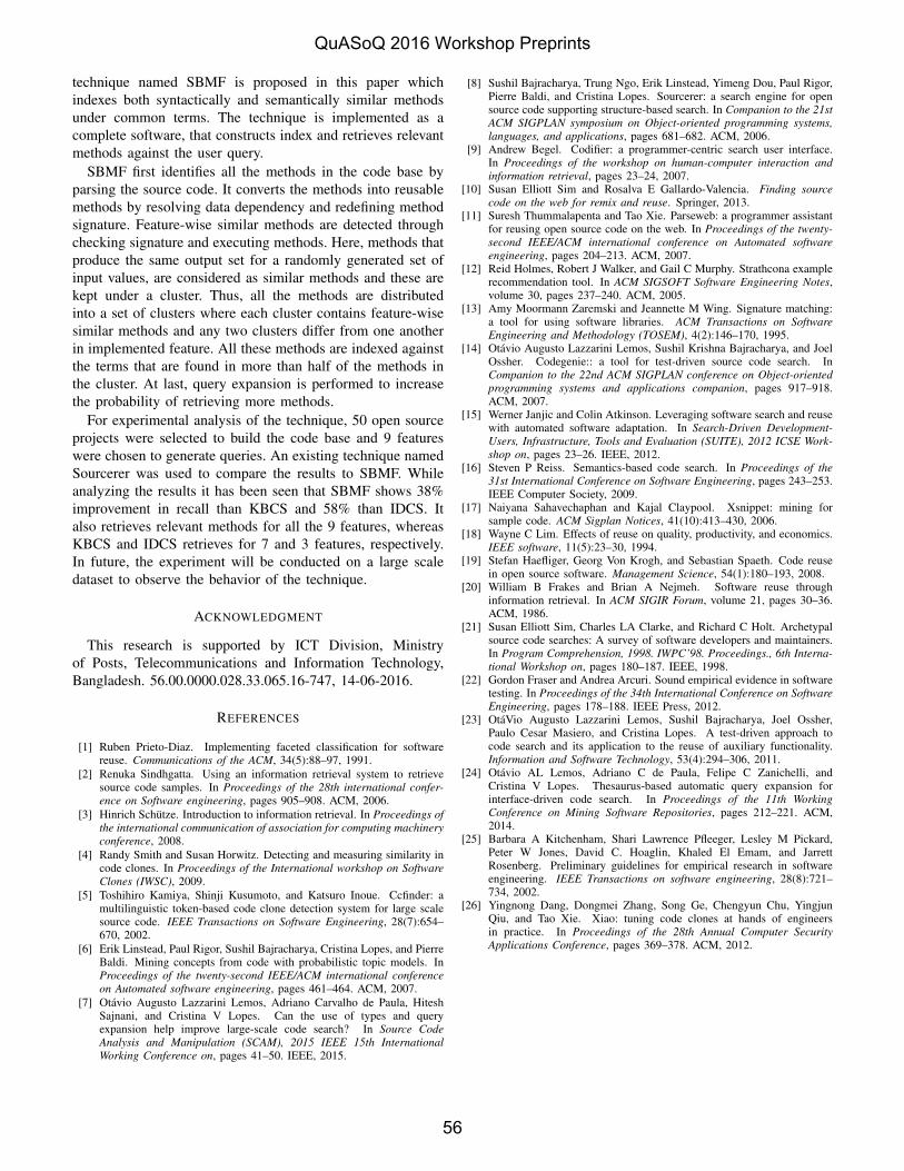
technique named SBMF is proposed in this paper whichindexes both syntactically and semantically similar methodsunder common terms. The technique is implemented as acomplete software, that constructs index and retrieves relevantmethods against the user query.

SBMF first identifies all the methods in the code base byparsing the source code. It converts the methods into reusablemethods by resolving data dependency and redefining methodsignature. Feature-wise similar methods are detected throughchecking signature and executing methods. Here, methods thatproduce the same output set for a randomly generated set ofinput values, are considered as similar methods and these arekept under a cluster. Thus, all the methods are distributedinto a set of clusters where each cluster contains feature-wisesimilar methods and any two clusters differ from one anotherin implemented feature. All these methods are indexed againstthe terms that are found in more than half of the methods inthe cluster. At last, query expansion is performed to increasethe probability of retrieving more methods.

For experimental analysis of the technique, 50 open sourceprojects were selected to build the code base and 9 featureswere chosen to generate queries. An existing technique namedSourcerer was used to compare the results to SBMF. Whileanalyzing the results it has been seen that SBMF shows 38%improvement in recall than KBCS and 58% than IDCS. Italso retrieves relevant methods for all the 9 features, whereasKBCS and IDCS retrieves for 7 and 3 features, respectively.In future, the experiment will be conducted on a large scaledataset to observe the behavior of the technique.

ACKNOWLEDGMENT

This research is supported by ICT Division, Ministryof Posts, Telecommunications and Information Technology,Bangladesh. 56.00.0000.028.33.065.16-747, 14-06-2016.

REFERENCES

[1] Ruben Prieto-Diaz. Implementing faceted classification for softwarereuse. Communications of the ACM, 34(5):88–97, 1991.

[2] Renuka Sindhgatta. Using an information retrieval system to retrievesource code samples. In Proceedings of the 28th international confer-ence on Software engineering, pages 905–908. ACM, 2006.

[3] Hinrich Schutze. Introduction to information retrieval. In Proceedings ofthe international communication of association for computing machineryconference, 2008.

[4] Randy Smith and Susan Horwitz. Detecting and measuring similarity incode clones. In Proceedings of the International workshop on SoftwareClones (IWSC), 2009.

[5] Toshihiro Kamiya, Shinji Kusumoto, and Katsuro Inoue. Ccfinder: amultilinguistic token-based code clone detection system for large scalesource code. IEEE Transactions on Software Engineering, 28(7):654–670, 2002.

[6] Erik Linstead, Paul Rigor, Sushil Bajracharya, Cristina Lopes, and PierreBaldi. Mining concepts from code with probabilistic topic models. InProceedings of the twenty-second IEEE/ACM international conferenceon Automated software engineering, pages 461–464. ACM, 2007.

[7] Otavio Augusto Lazzarini Lemos, Adriano Carvalho de Paula, HiteshSajnani, and Cristina V Lopes. Can the use of types and queryexpansion help improve large-scale code search? In Source CodeAnalysis and Manipulation (SCAM), 2015 IEEE 15th InternationalWorking Conference on, pages 41–50. IEEE, 2015.

[8] Sushil Bajracharya, Trung Ngo, Erik Linstead, Yimeng Dou, Paul Rigor,Pierre Baldi, and Cristina Lopes. Sourcerer: a search engine for opensource code supporting structure-based search. In Companion to the 21stACM SIGPLAN symposium on Object-oriented programming systems,languages, and applications, pages 681–682. ACM, 2006.

[9] Andrew Begel. Codifier: a programmer-centric search user interface.In Proceedings of the workshop on human-computer interaction andinformation retrieval, pages 23–24, 2007.

[10] Susan Elliott Sim and Rosalva E Gallardo-Valencia. Finding sourcecode on the web for remix and reuse. Springer, 2013.

[11] Suresh Thummalapenta and Tao Xie. Parseweb: a programmer assistantfor reusing open source code on the web. In Proceedings of the twenty-second IEEE/ACM international conference on Automated softwareengineering, pages 204–213. ACM, 2007.

[12] Reid Holmes, Robert J Walker, and Gail C Murphy. Strathcona examplerecommendation tool. In ACM SIGSOFT Software Engineering Notes,volume 30, pages 237–240. ACM, 2005.

[13] Amy Moormann Zaremski and Jeannette M Wing. Signature matching:a tool for using software libraries. ACM Transactions on SoftwareEngineering and Methodology (TOSEM), 4(2):146–170, 1995.

[14] Otavio Augusto Lazzarini Lemos, Sushil Krishna Bajracharya, and JoelOssher. Codegenie:: a tool for test-driven source code search. InCompanion to the 22nd ACM SIGPLAN conference on Object-orientedprogramming systems and applications companion, pages 917–918.ACM, 2007.

[15] Werner Janjic and Colin Atkinson. Leveraging software search and reusewith automated software adaptation. In Search-Driven Development-Users, Infrastructure, Tools and Evaluation (SUITE), 2012 ICSE Work-shop on, pages 23–26. IEEE, 2012.

[16] Steven P Reiss. Semantics-based code search. In Proceedings of the31st International Conference on Software Engineering, pages 243–253.IEEE Computer Society, 2009.

[17] Naiyana Sahavechaphan and Kajal Claypool. Xsnippet: mining forsample code. ACM Sigplan Notices, 41(10):413–430, 2006.

[18] Wayne C Lim. Effects of reuse on quality, productivity, and economics.IEEE software, 11(5):23–30, 1994.

[19] Stefan Haefliger, Georg Von Krogh, and Sebastian Spaeth. Code reusein open source software. Management Science, 54(1):180–193, 2008.

[20] William B Frakes and Brian A Nejmeh. Software reuse throughinformation retrieval. In ACM SIGIR Forum, volume 21, pages 30–36.ACM, 1986.

[21] Susan Elliott Sim, Charles LA Clarke, and Richard C Holt. Archetypalsource code searches: A survey of software developers and maintainers.In Program Comprehension, 1998. IWPC’98. Proceedings., 6th Interna-tional Workshop on, pages 180–187. IEEE, 1998.

[22] Gordon Fraser and Andrea Arcuri. Sound empirical evidence in softwaretesting. In Proceedings of the 34th International Conference on SoftwareEngineering, pages 178–188. IEEE Press, 2012.

[23] OtaVio Augusto Lazzarini Lemos, Sushil Bajracharya, Joel Ossher,Paulo Cesar Masiero, and Cristina Lopes. A test-driven approach tocode search and its application to the reuse of auxiliary functionality.Information and Software Technology, 53(4):294–306, 2011.

[24] Otavio AL Lemos, Adriano C de Paula, Felipe C Zanichelli, andCristina V Lopes. Thesaurus-based automatic query expansion forinterface-driven code search. In Proceedings of the 11th WorkingConference on Mining Software Repositories, pages 212–221. ACM,2014.

[25] Barbara A Kitchenham, Shari Lawrence Pfleeger, Lesley M Pickard,Peter W Jones, David C. Hoaglin, Khaled El Emam, and JarrettRosenberg. Preliminary guidelines for empirical research in softwareengineering. IEEE Transactions on software engineering, 28(8):721–734, 2002.

[26] Yingnong Dang, Dongmei Zhang, Song Ge, Chengyun Chu, YingjunQiu, and Tao Xie. Xiao: tuning code clones at hands of engineersin practice. In Proceedings of the 28th Annual Computer SecurityApplications Conference, pages 369–378. ACM, 2012.


56

workshop preprints quasoq 2016 - swc preprints quasoq 2016. 4. th. international workshop on...

Documents