worm algorithms - ustc
TRANSCRIPT

Outline Worm algorithms for Ising high-temperature graphs Worm algorithms for fully-packed loops Summary
Worm Algorithms
Youjin Deng
Department of Modern PhysicsUniversity of Science and Technology of China
P.R.China
November 6Hefei

Outline Worm algorithms for Ising high-temperature graphs Worm algorithms for fully-packed loops Summary
Outline
References/Collaborators
1. Youjin Deng, Timothy M. Garoni, and Alan D. Sokal,Dynamic Critical Behavior of the Worm Algorithm for the Ising Model,Phys. Rev. Lett. 99, 110601 (2007).
2. Wei Zhang, Timothy M. Garoni, and Youjin Deng,Simulating the fully-packed loop model on the honeycomb lattice with aworm algorithm, preprint.

Outline Worm algorithms for Ising high-temperature graphs Worm algorithms for fully-packed loops Summary
Outline
How do we efficiently simulate models near criticality?
◮ Problem: critical slowing-down

Outline Worm algorithms for Ising high-temperature graphs Worm algorithms for fully-packed loops Summary
Outline
How do we efficiently simulate models near criticality?
◮ Problem: critical slowing-down◮ The current state-of-the-art: cluster algorithms
◮ Swendsen & Wang PRL 1987◮ Use global moves in clever way
◮ More recent idea: worm algorithms◮ Prokof’ev & Svistunov PRL 2001◮ Enlarge an Eulerian configuration space to include defects◮ Move the defects via random walk
Outline Worm algorithms for Ising high-temperature graphs Worm algorithms for fully-packed loops Summary
High-temperature expansions, state spaces, worm dynamics . . .
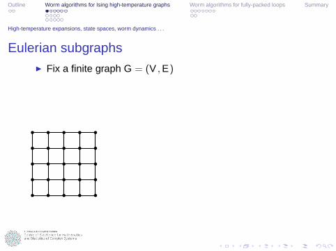
Eulerian subgraphs◮ Fix a finite graph G = (V , E)

Outline Worm algorithms for Ising high-temperature graphs Worm algorithms for fully-packed loops Summary
High-temperature expansions, state spaces, worm dynamics . . .
Eulerian subgraphs◮ Fix a finite graph G = (V , E)
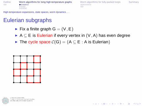
◮ A ⊆ E is Eulerian if every vertex in (V , A) has even degree
Outline Worm algorithms for Ising high-temperature graphs Worm algorithms for fully-packed loops Summary
High-temperature expansions, state spaces, worm dynamics . . .
Eulerian subgraphs◮ Fix a finite graph G = (V , E)
◮ A ⊆ E is Eulerian if every vertex in (V , A) has even degree◮ The cycle space C(G) = {A ⊆ E : A is Eulerian}

Outline Worm algorithms for Ising high-temperature graphs Worm algorithms for fully-packed loops Summary
High-temperature expansions, state spaces, worm dynamics . . .
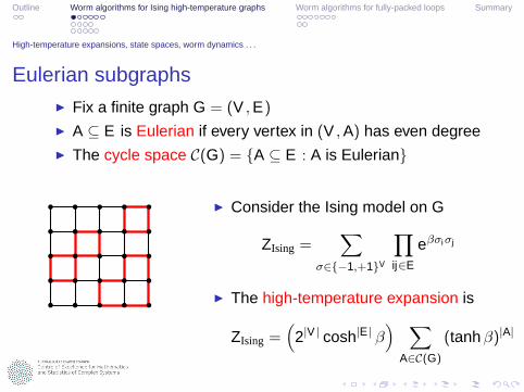
Eulerian subgraphs◮ Fix a finite graph G = (V , E)
◮ A ⊆ E is Eulerian if every vertex in (V , A) has even degree◮ The cycle space C(G) = {A ⊆ E : A is Eulerian}
◮ Consider the Ising model on G
ZIsing =∑
σ∈{−1,+1}V
∏
ij∈E
eβσiσj
Outline Worm algorithms for Ising high-temperature graphs Worm algorithms for fully-packed loops Summary
High-temperature expansions, state spaces, worm dynamics . . .
Eulerian subgraphs◮ Fix a finite graph G = (V , E)
◮ A ⊆ E is Eulerian if every vertex in (V , A) has even degree◮ The cycle space C(G) = {A ⊆ E : A is Eulerian}
◮ Consider the Ising model on G
ZIsing =∑
σ∈{−1,+1}V
∏
ij∈E
eβσiσj
◮ The high-temperature expansion is
ZIsing =(
2|V | cosh|E | β) ∑
A∈C(G)
(tanh β)|A|
Outline Worm algorithms for Ising high-temperature graphs Worm algorithms for fully-packed loops Summary
High-temperature expansions, state spaces, worm dynamics . . .
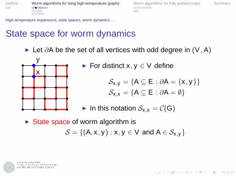
State space for worm dynamics
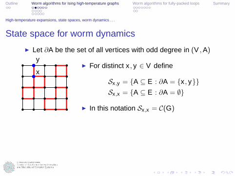
◮ Let ∂A be the set of all vertices with odd degree in (V , A)
x
y◮ For distinct x , y ∈ V define
Sx ,y = {A ⊆ E : ∂A = {x , y}}
Sx ,x = {A ⊆ E : ∂A = ∅}
◮ In this notation Sx ,x = C(G)
Outline Worm algorithms for Ising high-temperature graphs Worm algorithms for fully-packed loops Summary
High-temperature expansions, state spaces, worm dynamics . . .
State space for worm dynamics
◮ Let ∂A be the set of all vertices with odd degree in (V , A)
x
y◮ For distinct x , y ∈ V define
Sx ,y = {A ⊆ E : ∂A = {x , y}}
Sx ,x = {A ⊆ E : ∂A = ∅}
◮ In this notation Sx ,x = C(G)
◮ State space of worm algorithm is
S = {(A, x , y) : x , y ∈ V and A ∈ Sx ,y}
◮ Assign (A, x , y) ∈ S probability
π(A, x , y) ∝ dx dy (tanh β)|A|
Outline Worm algorithms for Ising high-temperature graphs Worm algorithms for fully-packed loops Summary
High-temperature expansions, state spaces, worm dynamics . . .
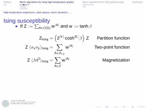
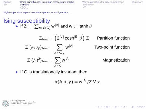
Ising susceptibility◮ If Z :=
∑A∈C(G) w |A| and w := tanh β
ZIsing =(
2|V | cosh|E | β)
Z Partition function
Z 〈σxσy 〉Ising =∑
A∈Sx,y
w |A| Two-point function
Z 〈M2〉Ising =∑
A∈S
w |A| Magnetization
Outline Worm algorithms for Ising high-temperature graphs Worm algorithms for fully-packed loops Summary
High-temperature expansions, state spaces, worm dynamics . . .
Ising susceptibility◮ If Z :=
∑A∈C(G) w |A| and w := tanh β
ZIsing =(
2|V | cosh|E | β)
Z Partition function
Z 〈σxσy 〉Ising =∑
A∈Sx,y
w |A| Two-point function
Z 〈M2〉Ising =∑
A∈S
w |A| Magnetization
◮ If G is translationally invariant then
π(A, x , y) = w |A|/Z V χ
◮ Therefore the observable D0(A, x , y) = δx ,y satisfies
〈D0〉π = 1/χ

Outline Worm algorithms for Ising high-temperature graphs Worm algorithms for fully-packed loops Summary
High-temperature expansions, state spaces, worm dynamics . . .
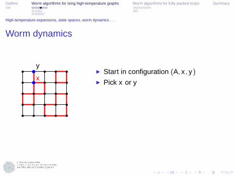
Worm dynamics
x
y◮ Start in configuration (A, x , y)
Outline Worm algorithms for Ising high-temperature graphs Worm algorithms for fully-packed loops Summary
High-temperature expansions, state spaces, worm dynamics . . .
Worm dynamics
x
y◮ Start in configuration (A, x , y)
◮ Pick x or y

Outline Worm algorithms for Ising high-temperature graphs Worm algorithms for fully-packed loops Summary
High-temperature expansions, state spaces, worm dynamics . . .
Worm dynamics
x x ′
y◮ Start in configuration (A, x , y)
◮ Pick x or y◮ Pick x ′ ∼ x

Outline Worm algorithms for Ising high-temperature graphs Worm algorithms for fully-packed loops Summary
High-temperature expansions, state spaces, worm dynamics . . .
Worm dynamics
x
y
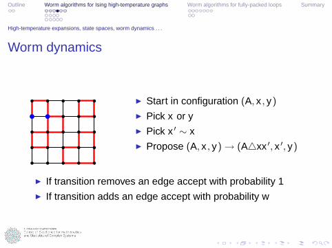
x ′◮ Start in configuration (A, x , y)
◮ Pick x or y◮ Pick x ′ ∼ x◮ Propose (A, x , y) → (A△xx ′, x ′, y)
◮ If transition removes an edge accept with probability 1

Outline Worm algorithms for Ising high-temperature graphs Worm algorithms for fully-packed loops Summary
High-temperature expansions, state spaces, worm dynamics . . .
Worm dynamics
x
y
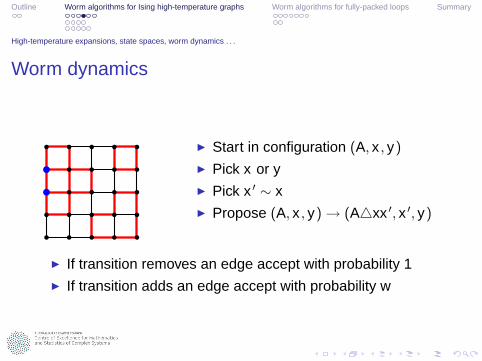
x ′◮ Start in configuration (A, x , y)
◮ Pick x or y◮ Pick x ′ ∼ x◮ Propose (A, x , y) → (A△xx ′, x ′, y)
◮ If transition removes an edge accept with probability 1◮ If transition adds an edge accept with probability w

Outline Worm algorithms for Ising high-temperature graphs Worm algorithms for fully-packed loops Summary
High-temperature expansions, state spaces, worm dynamics . . .
Worm dynamics
◮ Start in configuration (A, x , y)
◮ Pick x or y◮ Pick x ′ ∼ x◮ Propose (A, x , y) → (A△xx ′, x ′, y)
◮ If transition removes an edge accept with probability 1◮ If transition adds an edge accept with probability w

Outline Worm algorithms for Ising high-temperature graphs Worm algorithms for fully-packed loops Summary
High-temperature expansions, state spaces, worm dynamics . . .
Transition matrix
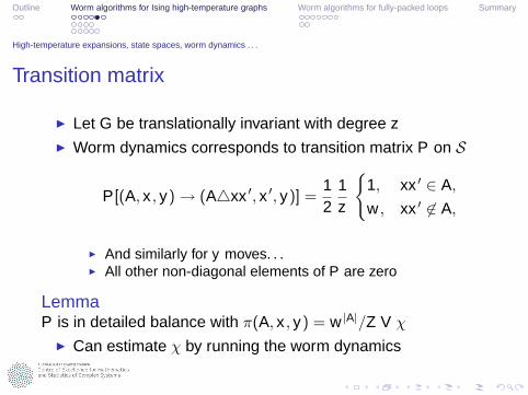
◮ Let G be translationally invariant with degree z◮ Worm dynamics corresponds to transition matrix P on S
P[(A, x , y) → (A△xx ′, x ′, y)] =12
1z
{1, xx ′ ∈ A,
w , xx ′ 6∈ A,
◮ And similarly for y moves. . .◮ All other non-diagonal elements of P are zero
Outline Worm algorithms for Ising high-temperature graphs Worm algorithms for fully-packed loops Summary
High-temperature expansions, state spaces, worm dynamics . . .
Transition matrix
◮ Let G be translationally invariant with degree z◮ Worm dynamics corresponds to transition matrix P on S
P[(A, x , y) → (A△xx ′, x ′, y)] =12
1z
{1, xx ′ ∈ A,
w , xx ′ 6∈ A,
◮ And similarly for y moves. . .◮ All other non-diagonal elements of P are zero
LemmaP is in detailed balance with π(A, x , y) = w |A|/Z V χ
◮ Can estimate χ by running the worm dynamics

Outline Worm algorithms for Ising high-temperature graphs Worm algorithms for fully-packed loops Summary
High-temperature expansions, state spaces, worm dynamics . . .
Efficiency
◮ Worm dynamics provide a valid way to compute χ

Outline Worm algorithms for Ising high-temperature graphs Worm algorithms for fully-packed loops Summary
High-temperature expansions, state spaces, worm dynamics . . .
Efficiency
◮ Worm dynamics provide a valid way to compute χ
◮ But how efficient is the worm algorithm?

Outline Worm algorithms for Ising high-temperature graphs Worm algorithms for fully-packed loops Summary
High-temperature expansions, state spaces, worm dynamics . . .
Efficiency
◮ Worm dynamics provide a valid way to compute χ
◮ But how efficient is the worm algorithm?◮ How do we measure efficiency anyway?
Outline Worm algorithms for Ising high-temperature graphs Worm algorithms for fully-packed loops Summary
High-temperature expansions, state spaces, worm dynamics . . .
Efficiency
◮ Worm dynamics provide a valid way to compute χ
◮ But how efficient is the worm algorithm?◮ How do we measure efficiency anyway?◮ Empirically – measuring autocorrelations

Outline Worm algorithms for Ising high-temperature graphs Worm algorithms for fully-packed loops Summary
Autocorrelations, critical slowing down . . .
Markov-chain Monte Carlo◮ Markov chain
◮ State space S, with |S| < ∞◮ Transition matrix P◮ Stationary distribution π

Outline Worm algorithms for Ising high-temperature graphs Worm algorithms for fully-packed loops Summary
Autocorrelations, critical slowing down . . .
Markov-chain Monte Carlo◮ Markov chain
◮ State space S, with |S| < ∞◮ Transition matrix P◮ Stationary distribution π
◮ Observables (random variables) X , Y , . . .
◮ Simulate Markov chain s0P−→ s1
P−→ s2
P−→ . . . with st ∈ S
◮ Get time series X0, X1, X2, . . . with Xt = X (st)
◮ Define the autocorrelation function
ρX (t) :=〈XsXs+t〉π − 〈X 〉2
π
varπ(X )
◮ Stationary process – start “in equilibrium”
Outline Worm algorithms for Ising high-temperature graphs Worm algorithms for fully-packed loops Summary
Autocorrelations, critical slowing down . . .
Integrated autocorrelation times
◮ The integrated autocorrelation time
τint,X :=12
∞∑
t=−∞
ρX (t)

Outline Worm algorithms for Ising high-temperature graphs Worm algorithms for fully-packed loops Summary
Autocorrelations, critical slowing down . . .
Integrated autocorrelation times
◮ The integrated autocorrelation time
τint,X :=12
∞∑
t=−∞
ρX (t)
◮ If X̂ is the sample mean of {Xt}Tt=1 then we have
var(X̂ ) ∼ 2 τint,Xvar(X )
T, T → ∞
◮ 1 “effectively independent” observation every 2 τint,X steps

Outline Worm algorithms for Ising high-temperature graphs Worm algorithms for fully-packed loops Summary
Autocorrelations, critical slowing down . . .
Exponential autocorrelation times
◮ ρX (t) typically decays exponentially as t → ∞
◮ The exponential autocorrelation time
τexp,X := lim supt→∞
t− log |ρX (t)|
and τexp := supX
τexp,X
◮ Typically τexp,X = τexp < ∞ and τint,X ≤ τexp for all X
◮ Start the chain with arbitrary distribution α
◮ Distribution at time t is αP t
LemmaαP t tends to π with rate bounded by e−t/τexp

Outline Worm algorithms for Ising high-temperature graphs Worm algorithms for fully-packed loops Summary
Autocorrelations, critical slowing down . . .
Critical slowing-down
◮ Near a critical point the autocorrelation times typicallydiverge like
τ ∼ ξz
Outline Worm algorithms for Ising high-temperature graphs Worm algorithms for fully-packed loops Summary
Autocorrelations, critical slowing down . . .
Critical slowing-down
◮ Near a critical point the autocorrelation times typicallydiverge like
τ ∼ ξz
◮ More precisely, we have a family of exponents:zexp, and zint,X for each observable X .
◮ Different algorithms for the same model can have verydifferent z
◮ E.g. d = 2 Ising model◮ Glauber (Metropolis) algorithm z ≈ 2◮ Swendsen-Wang algorithm z ≈ 0.2
Outline Worm algorithms for Ising high-temperature graphs Worm algorithms for fully-packed loops Summary
Numerical results
Worm simulations
◮ Simulated the critical square-lattice Ising model

Outline Worm algorithms for Ising high-temperature graphs Worm algorithms for fully-packed loops Summary
Numerical results
Worm simulations
◮ Simulated the critical square-lattice Ising model◮ Focus on two observables:
◮ N (A, x , y) = |A|◮ D0(A, x , y) = δx,y
◮ 〈N〉 is “energy-like”◮ 〈D0〉 = 1/χ

Outline Worm algorithms for Ising high-temperature graphs Worm algorithms for fully-packed loops Summary
Numerical results
Worm simulations
◮ Simulated the critical square-lattice Ising model◮ Focus on two observables:
◮ N (A, x , y) = |A|◮ D0(A, x , y) = δx,y
◮ 〈N〉 is “energy-like”◮ 〈D0〉 = 1/χ
◮ Measured observables after every hit (worm update)◮ Natural unit of time is one sweep (Ld hits)
Outline Worm algorithms for Ising high-temperature graphs Worm algorithms for fully-packed loops Summary
Numerical results
Dynamics of N
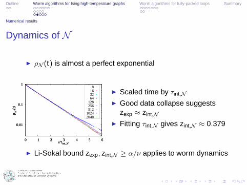
◮ ρN (t) is almost a perfect exponential
0.01
0.1
1
0 1 2 3 4 5 6
ρ N (
t)
t/τint,N
0.01
0.1
1
0 1 2 3 4 5 6
ρ N (
t)
t/τint,N
8 16 32 64
128 256 512
10242048
◮ Scaled time by τint,N
◮ Good data collapse suggestszexp ≈ zint,N
◮ Fitting τint,N gives zint,N ≈ 0.379
◮ Li-Sokal bound zexp, zint,N ≥ α/ν applies to worm dynamics

Outline Worm algorithms for Ising high-temperature graphs Worm algorithms for fully-packed loops Summary
Numerical results
Dynamics of D0
◮ ρD0(t) decays significantly in O(1) hits!
10-6
10-5
10-4
10-3
10-2
10-1
1
10710610510410310210 1
ρ D0 (
t)
t
L increases
10-6
10-5
10-4
10-3
10-2
10-1
1
10710610510410310210 1
ρ D0 (
t)
t
L increases
8 16 32 64
128 256 512
10242048 ◮ ρD0(t) ∼ t−s with s ≈ 0.75
◮ D0 decorrelates on a totally different time scale to N
Outline Worm algorithms for Ising high-temperature graphs Worm algorithms for fully-packed loops Summary
Numerical results
Three dimensions
◮ Qualitatively similar behavior when d = 3:

Outline Worm algorithms for Ising high-temperature graphs Worm algorithms for fully-packed loops Summary
Numerical results
Three dimensions
◮ Qualitatively similar behavior when d = 3:◮ ρD0(t) ∼ t−s
◮ s ≈ 0.66
Outline Worm algorithms for Ising high-temperature graphs Worm algorithms for fully-packed loops Summary
Numerical results
Three dimensions
◮ Qualitatively similar behavior when d = 3:◮ ρD0(t) ∼ t−s
◮ s ≈ 0.66◮ ρN (t) roughly exponential◮ zexp ≈ zint,N ≈ α/ν ≈ 0.174◮ Li-Sokal bound may be sharp for d = 3 worm algorithm
Outline Worm algorithms for Ising high-temperature graphs Worm algorithms for fully-packed loops Summary
Numerical results
Three dimensions
◮ Qualitatively similar behavior when d = 3:◮ ρD0(t) ∼ t−s
◮ s ≈ 0.66◮ ρN (t) roughly exponential◮ zexp ≈ zint,N ≈ α/ν ≈ 0.174◮ Li-Sokal bound may be sharp for d = 3 worm algorithm◮ Compare Swendsen-Wang zSW ≈ 0.46

Outline Worm algorithms for Ising high-temperature graphs Worm algorithms for fully-packed loops Summary
Numerical results
Practical efficiency for square/cubic lattice critical Ising
◮ Swendsen-Wang seems to outperform worm when d = 2
Outline Worm algorithms for Ising high-temperature graphs Worm algorithms for fully-packed loops Summary
Numerical results
Practical efficiency for square/cubic lattice critical Ising
◮ Swendsen-Wang seems to outperform worm when d = 2◮ Efficiency depends on observable, X
Outline Worm algorithms for Ising high-temperature graphs Worm algorithms for fully-packed loops Summary
Numerical results
Practical efficiency for square/cubic lattice critical Ising
◮ Swendsen-Wang seems to outperform worm when d = 2◮ Efficiency depends on observable, X◮ A simple way to compare worm and SW is to compute
κ = TCPU varX̂ for both algorithms

Outline Worm algorithms for Ising high-temperature graphs Worm algorithms for fully-packed loops Summary
Numerical results
Practical efficiency for square/cubic lattice critical Ising
◮ Swendsen-Wang seems to outperform worm when d = 2◮ Efficiency depends on observable, X◮ A simple way to compare worm and SW is to compute
κ = TCPU varX̂ for both algorithms◮ When d = 3 and X = D0 we find κworm/κSW ≈ L−0.33
◮ With the crossover κworm/κSW ≈ 1 at around L ≈ 20
◮ There is also a natural worm estimator for ξ
◮ Again SW outperforms worm when d = 2

Outline Worm algorithms for Ising high-temperature graphs Worm algorithms for fully-packed loops Summary
Numerical results
Practical efficiency for square/cubic lattice critical Ising
◮ Swendsen-Wang seems to outperform worm when d = 2◮ Efficiency depends on observable, X◮ A simple way to compare worm and SW is to compute
κ = TCPU varX̂ for both algorithms◮ When d = 3 and X = D0 we find κworm/κSW ≈ L−0.33
◮ With the crossover κworm/κSW ≈ 1 at around L ≈ 20
◮ There is also a natural worm estimator for ξ
◮ Again SW outperforms worm when d = 2◮ For d = 3 we find κworm/κSW ≈ L−0.32
◮ With the crossover κworm/κSW ≈ 1 at around L ≈ 45

Outline Worm algorithms for Ising high-temperature graphs Worm algorithms for fully-packed loops Summary
An alternate perspective on worm dynamics
An alternative perspective on worm dynamics◮ Our perspective so far:
Worm algorithm ⇐⇒ simulate Ising high-temperature graphs
Outline Worm algorithms for Ising high-temperature graphs Worm algorithms for fully-packed loops Summary
An alternate perspective on worm dynamics
An alternative perspective on worm dynamics◮ Our perspective so far:
Worm algorithm ⇐⇒ simulate Ising high-temperature graphs
◮ Eulerian-subgraph model

Outline Worm algorithms for Ising high-temperature graphs Worm algorithms for fully-packed loops Summary
An alternate perspective on worm dynamics
An alternative perspective on worm dynamics◮ Our perspective so far:
Worm algorithm ⇐⇒ simulate Ising high-temperature graphs
◮ Eulerian-subgraph model◮ State space C(G)
Outline Worm algorithms for Ising high-temperature graphs Worm algorithms for fully-packed loops Summary
An alternate perspective on worm dynamics
An alternative perspective on worm dynamics◮ Our perspective so far:
Worm algorithm ⇐⇒ simulate Ising high-temperature graphs
◮ Eulerian-subgraph model◮ State space C(G)◮ P(A) ∝ w |A|
◮ Run a worm simulation

Outline Worm algorithms for Ising high-temperature graphs Worm algorithms for fully-packed loops Summary
An alternate perspective on worm dynamics
An alternative perspective on worm dynamics◮ Our perspective so far:
Worm algorithm ⇐⇒ simulate Ising high-temperature graphs
◮ Eulerian-subgraph model◮ State space C(G)◮ P(A) ∝ w |A|
◮ Run a worm simulation◮ Only observe the chain when A ∈ C(G), i.e. when x = y

Outline Worm algorithms for Ising high-temperature graphs Worm algorithms for fully-packed loops Summary
An alternate perspective on worm dynamics
An alternative perspective on worm dynamics◮ Our perspective so far:
Worm algorithm ⇐⇒ simulate Ising high-temperature graphs
◮ Eulerian-subgraph model◮ State space C(G)◮ P(A) ∝ w |A|
◮ Run a worm simulation◮ Only observe the chain when A ∈ C(G), i.e. when x = y◮ Obtain a new Markov chain P◮ Stationary distribution π(A, x , x) ∝ f (x) w |A|
◮ New perspective:
Worm algorithm ⇐⇒ simulate Eulerian-subgraph model

Outline Worm algorithms for Ising high-temperature graphs Worm algorithms for fully-packed loops Summary
An alternate perspective on worm dynamics
Loop models
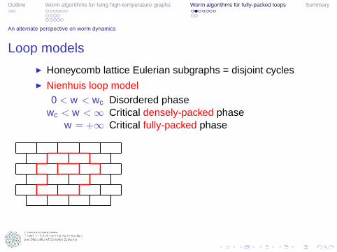
◮ Honeycomb lattice Eulerian subgraphs = disjoint cycles◮ Nienhuis loop model
Outline Worm algorithms for Ising high-temperature graphs Worm algorithms for fully-packed loops Summary
An alternate perspective on worm dynamics
Loop models
◮ Honeycomb lattice Eulerian subgraphs = disjoint cycles◮ Nienhuis loop model
0 < w < wc Disordered phasewc < w < ∞ Critical densely-packed phase
w = +∞ Critical fully-packed phase
+ + + ++ − − + +
+ − − ++ − + − +
+ − − ++ + + + + ◮ 1 loop config ↔ 2 dual spin configs
◮ Ising spin domains

Outline Worm algorithms for Ising high-temperature graphs Worm algorithms for fully-packed loops Summary
An alternate perspective on worm dynamics
Loop models
◮ Honeycomb lattice Eulerian subgraphs = disjoint cycles◮ Nienhuis loop model
0 < w < wc Disordered phasewc < w < ∞ Critical densely-packed phase
w = +∞ Critical fully-packed phase
+ + + ++ − − + +
+ − − ++ − + − +
+ − − ++ + + + + ◮ 1 loop config ↔ 2 dual spin configs
◮ Ising spin domains◮ w = e−2β
◮ w > 1 =⇒ antiferromagnetic β
◮ Worm ⇐⇒ simulate dual Ising domain boundaries

Outline Worm algorithms for Ising high-temperature graphs Worm algorithms for fully-packed loops Summary
An alternate perspective on worm dynamics
Fully-packed loop model (FPL)

Outline Worm algorithms for Ising high-temperature graphs Worm algorithms for fully-packed loops Summary
An alternate perspective on worm dynamics
Fully-packed loop model (FPL)
◮ FPL ↔ triangular-lattice Ising antiferromagnet at T = 0

Outline Worm algorithms for Ising high-temperature graphs Worm algorithms for fully-packed loops Summary
An alternate perspective on worm dynamics
Fully-packed loop model (FPL)
+−
+
Frustration
◮ FPL ↔ triangular-lattice Ising antiferromagnet at T = 0◮ Frustrated systems hard to simulate

Outline Worm algorithms for Ising high-temperature graphs Worm algorithms for fully-packed loops Summary
An alternate perspective on worm dynamics
Fully-packed loop model (FPL)
+−
+
Frustration
◮ FPL ↔ triangular-lattice Ising antiferromagnet at T = 0◮ Frustrated systems hard to simulate◮ Cluster algorithms for frustrated Ising models thought to be
non-ergodic at T = 0

Outline Worm algorithms for Ising high-temperature graphs Worm algorithms for fully-packed loops Summary
An alternate perspective on worm dynamics
Fully-packed loop model (FPL)
+−
+
Frustration
◮ FPL ↔ triangular-lattice Ising antiferromagnet at T = 0◮ Frustrated systems hard to simulate◮ Cluster algorithms for frustrated Ising models thought to be
non-ergodic at T = 0◮ Can we use worm instead?

Outline Worm algorithms for Ising high-temperature graphs Worm algorithms for fully-packed loops Summary
An alternate perspective on worm dynamics
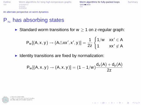
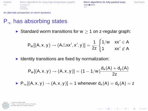
P∞ has absorbing states
◮ Standard worm transitions for w ≥ 1 on z-regular graph:
Pw [(A, x , y) → (A△xx ′, x ′, y)] =1
2z
{1/w xx ′ ∈ A
1 xx ′ 6∈ A
Outline Worm algorithms for Ising high-temperature graphs Worm algorithms for fully-packed loops Summary
An alternate perspective on worm dynamics
P∞ has absorbing states
◮ Standard worm transitions for w ≥ 1 on z-regular graph:
Pw [(A, x , y) → (A△xx ′, x ′, y)] =1
2z
{1/w xx ′ ∈ A
1 xx ′ 6∈ A
◮ Identity transitions are fixed by normalization:
Pw [(A, x , y) → (A, x , y)] = (1 − 1/w)dx(A) + dy (A)
2z
◮ P∞[(A, x , y) → (A, x , y)] = 1 whenever dx(A) = dy (A) = z

Outline Worm algorithms for Ising high-temperature graphs Worm algorithms for fully-packed loops Summary
An alternate perspective on worm dynamics
P∞ has absorbing states
◮ Standard worm transitions for w ≥ 1 on z-regular graph:
Pw [(A, x , y) → (A△xx ′, x ′, y)] =1
2z
{1/w xx ′ ∈ A
1 xx ′ 6∈ A
◮ Identity transitions are fixed by normalization:
Pw [(A, x , y) → (A, x , y)] = (1 − 1/w)dx(A) + dy (A)
2z
◮ P∞[(A, x , y) → (A, x , y)] = 1 whenever dx(A) = dy (A) = z◮ Cannot use standard worm algorithm when w = +∞

Outline Worm algorithms for Ising high-temperature graphs Worm algorithms for fully-packed loops Summary
An alternate perspective on worm dynamics
How do we solve the problem?
◮ P∞[(A, x , y) → (A, x , y)] = 1 whenever dx(A) = dy (A) = z

Outline Worm algorithms for Ising high-temperature graphs Worm algorithms for fully-packed loops Summary
An alternate perspective on worm dynamics
How do we solve the problem?
◮ P∞[(A, x , y) → (A, x , y)] = 1 whenever dx(A) = dy (A) = z◮ But on the honeycomb lattice z = 3
Outline Worm algorithms for Ising high-temperature graphs Worm algorithms for fully-packed loops Summary
An alternate perspective on worm dynamics
How do we solve the problem?
◮ P∞[(A, x , y) → (A, x , y)] = 1 whenever dx(A) = dy (A) = z◮ But on the honeycomb lattice z = 3◮ So states with Eulerian A never get stuck
Outline Worm algorithms for Ising high-temperature graphs Worm algorithms for fully-packed loops Summary
An alternate perspective on worm dynamics
How do we solve the problem?
◮ P∞[(A, x , y) → (A, x , y)] = 1 whenever dx(A) = dy (A) = z◮ But on the honeycomb lattice z = 3◮ So states with Eulerian A never get stuck◮ To simulate loop models, we only observe the chain when
A is Eulerian. . .

Outline Worm algorithms for Ising high-temperature graphs Worm algorithms for fully-packed loops Summary
An alternate perspective on worm dynamics
How do we solve the problem?
◮ P∞[(A, x , y) → (A, x , y)] = 1 whenever dx(A) = dy (A) = z◮ But on the honeycomb lattice z = 3◮ So states with Eulerian A never get stuck◮ To simulate loop models, we only observe the chain when
A is Eulerian. . .◮ Try defining new transition matrix P ′
∞ such that:

Outline Worm algorithms for Ising high-temperature graphs Worm algorithms for fully-packed loops Summary
An alternate perspective on worm dynamics
How do we solve the problem?
◮ P∞[(A, x , y) → (A, x , y)] = 1 whenever dx(A) = dy (A) = z◮ But on the honeycomb lattice z = 3◮ So states with Eulerian A never get stuck◮ To simulate loop models, we only observe the chain when
A is Eulerian. . .◮ Try defining new transition matrix P ′
∞ such that:◮ P ′
∞[(A, x , x) → · ] = limw→∞ Pw [(A, x , x) → · ]

Outline Worm algorithms for Ising high-temperature graphs Worm algorithms for fully-packed loops Summary
An alternate perspective on worm dynamics
How do we solve the problem?
◮ P∞[(A, x , y) → (A, x , y)] = 1 whenever dx(A) = dy (A) = z◮ But on the honeycomb lattice z = 3◮ So states with Eulerian A never get stuck◮ To simulate loop models, we only observe the chain when
A is Eulerian. . .◮ Try defining new transition matrix P ′
∞ such that:◮ P ′
∞[(A, x , x) → · ] = limw→∞ Pw [(A, x , x) → · ]◮ P ′
∞[(A, x , y) → (A, x , y)] = 0 when x 6= y
◮ This will get rid of the absorbing states. . .

Outline Worm algorithms for Ising high-temperature graphs Worm algorithms for fully-packed loops Summary
An alternate perspective on worm dynamics
How do we solve the problem?
◮ P∞[(A, x , y) → (A, x , y)] = 1 whenever dx(A) = dy (A) = z◮ But on the honeycomb lattice z = 3◮ So states with Eulerian A never get stuck◮ To simulate loop models, we only observe the chain when
A is Eulerian. . .◮ Try defining new transition matrix P ′
∞ such that:◮ P ′
∞[(A, x , x) → · ] = limw→∞ Pw [(A, x , x) → · ]◮ P ′
∞[(A, x , y) → (A, x , y)] = 0 when x 6= y
◮ This will get rid of the absorbing states. . .◮ If we are lucky P ′
∞ will simulate the FPL. . .

Outline Worm algorithms for Ising high-temperature graphs Worm algorithms for fully-packed loops Summary
An alternate perspective on worm dynamics
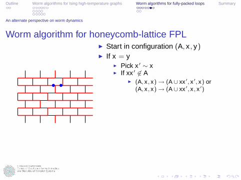
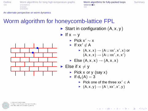
Worm algorithm for honeycomb-lattice FPL◮ Start in configuration (A, x , y)

Outline Worm algorithms for Ising high-temperature graphs Worm algorithms for fully-packed loops Summary
An alternate perspective on worm dynamics
Worm algorithm for honeycomb-lattice FPL◮ Start in configuration (A, x , y)
◮ If x = y

Outline Worm algorithms for Ising high-temperature graphs Worm algorithms for fully-packed loops Summary
An alternate perspective on worm dynamics
Worm algorithm for honeycomb-lattice FPL◮ Start in configuration (A, x , y)
◮ If x = y◮ Pick x ′ ∼ x
Outline Worm algorithms for Ising high-temperature graphs Worm algorithms for fully-packed loops Summary
An alternate perspective on worm dynamics
Worm algorithm for honeycomb-lattice FPL◮ Start in configuration (A, x , y)
◮ If x = y◮ Pick x ′ ∼ x◮ If xx ′ 6∈ A
◮ (A, x , x) → (A ∪ xx ′, x ′
, x) or(A, x , x) → (A ∪ xx ′
, x , x ′)
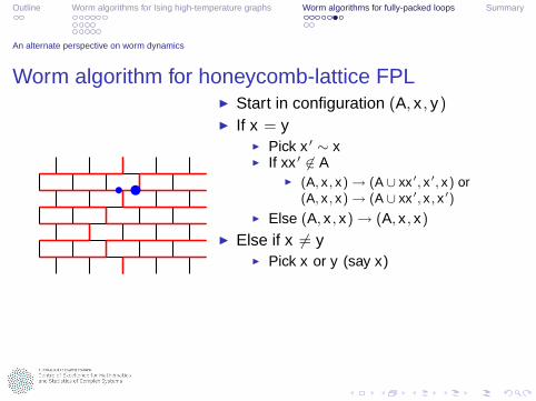
◮ Else (A, x , x) → (A, x , x)

Outline Worm algorithms for Ising high-temperature graphs Worm algorithms for fully-packed loops Summary
An alternate perspective on worm dynamics
Worm algorithm for honeycomb-lattice FPL◮ Start in configuration (A, x , y)
◮ If x = y◮ Pick x ′ ∼ x◮ If xx ′ 6∈ A
◮ (A, x , x) → (A ∪ xx ′, x ′
, x) or(A, x , x) → (A ∪ xx ′
, x , x ′)
◮ Else (A, x , x) → (A, x , x)
◮ Else if x 6= y
Outline Worm algorithms for Ising high-temperature graphs Worm algorithms for fully-packed loops Summary
An alternate perspective on worm dynamics
Worm algorithm for honeycomb-lattice FPL◮ Start in configuration (A, x , y)
◮ If x = y◮ Pick x ′ ∼ x◮ If xx ′ 6∈ A
◮ (A, x , x) → (A ∪ xx ′, x ′
, x) or(A, x , x) → (A ∪ xx ′
, x , x ′)
◮ Else (A, x , x) → (A, x , x)
◮ Else if x 6= y◮ Pick x or y (say x)

Outline Worm algorithms for Ising high-temperature graphs Worm algorithms for fully-packed loops Summary
An alternate perspective on worm dynamics
Worm algorithm for honeycomb-lattice FPL◮ Start in configuration (A, x , y)
◮ If x = y◮ Pick x ′ ∼ x◮ If xx ′ 6∈ A
◮ (A, x , x) → (A ∪ xx ′, x ′
, x) or(A, x , x) → (A ∪ xx ′
, x , x ′)
◮ Else (A, x , x) → (A, x , x)
◮ Else if x 6= y◮ Pick x or y (say x)◮ If dx(A) = 3
◮ Pick one of the three xx ′ ∈ A◮ (A, x , y) → (A \ xx ′
, x ′, y)
◮ Else if dx(A) = 1◮ Pick one of the two xx ′ 6∈ A◮ (A, x , y) → (A ∪ xx ′
, x ′, y)
Outline Worm algorithms for Ising high-temperature graphs Worm algorithms for fully-packed loops Summary
An alternate perspective on worm dynamics
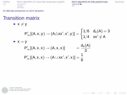
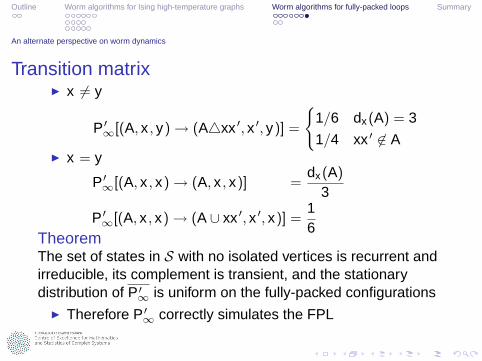
Transition matrix◮ x 6= y
P ′∞[(A, x , y) → (A△xx ′, x ′, y)] =
{1/6 dx(A) = 3
1/4 xx ′ 6∈ A◮ x = y
P ′∞[(A, x , x) → (A, x , x)] =
dx(A)
3
P ′∞[(A, x , x) → (A ∪ xx ′, x ′, x)] =
16

Outline Worm algorithms for Ising high-temperature graphs Worm algorithms for fully-packed loops Summary
An alternate perspective on worm dynamics
Transition matrix◮ x 6= y
P ′∞[(A, x , y) → (A△xx ′, x ′, y)] =
{1/6 dx(A) = 3
1/4 xx ′ 6∈ A◮ x = y
P ′∞[(A, x , x) → (A, x , x)] =
dx(A)
3
P ′∞[(A, x , x) → (A ∪ xx ′, x ′, x)] =
16
TheoremThe set of states in S with no isolated vertices is recurrent andirreducible, its complement is transient, and the stationarydistribution of P ′
∞ is uniform on the fully-packed configurations
Outline Worm algorithms for Ising high-temperature graphs Worm algorithms for fully-packed loops Summary
An alternate perspective on worm dynamics
Transition matrix◮ x 6= y
P ′∞[(A, x , y) → (A△xx ′, x ′, y)] =
{1/6 dx(A) = 3
1/4 xx ′ 6∈ A◮ x = y
P ′∞[(A, x , x) → (A, x , x)] =
dx(A)
3
P ′∞[(A, x , x) → (A ∪ xx ′, x ′, x)] =
16
TheoremThe set of states in S with no isolated vertices is recurrent andirreducible, its complement is transient, and the stationarydistribution of P ′
∞ is uniform on the fully-packed configurations◮ Therefore P ′
∞ correctly simulates the FPL
Outline Worm algorithms for Ising high-temperature graphs Worm algorithms for fully-packed loops Summary
Numerical results
Worm simulations of honeycomb-lattice FPL
◮ Simulated the honeycomb-lattice FPL

Outline Worm algorithms for Ising high-temperature graphs Worm algorithms for fully-packed loops Summary
Numerical results
Worm simulations of honeycomb-lattice FPL
◮ Simulated the honeycomb-lattice FPL◮ Again observed multiple time scales
Outline Worm algorithms for Ising high-temperature graphs Worm algorithms for fully-packed loops Summary
Numerical results
Worm simulations of honeycomb-lattice FPL
◮ Simulated the honeycomb-lattice FPL◮ Again observed multiple time scales◮ Nl(A, x , y) = number of loops (cyclomatic number)◮ 〈Nl〉 is “energy-like”

Outline Worm algorithms for Ising high-temperature graphs Worm algorithms for fully-packed loops Summary
Numerical results
Worm simulations of honeycomb-lattice FPL
◮ Simulated the honeycomb-lattice FPL◮ Again observed multiple time scales◮ Nl(A, x , y) = number of loops (cyclomatic number)◮ 〈Nl〉 is “energy-like”◮ Nl is the slowest mode observed

Outline Worm algorithms for Ising high-temperature graphs Worm algorithms for fully-packed loops Summary
Numerical results
Dynamics of Nl
◮ ρNl (t) is almost a perfect exponential
0.01
0.1
1
0 1 2 3 4 5 6 7 8
ρ Nl (
t)
t/τint,Nl
0.01
0.1
1
0 1 2 3 4 5 6 7 8
ρ Nl (
t)
t/τint,Nl
12 24 30 60 90150240600900
◮ Scaled time by τint,Nl
◮ Good data collapse suggestszexp ≈ zint,Nl
◮ Fitting τint,Nl giveszint,Nl = 0.515(8)

Outline Worm algorithms for Ising high-temperature graphs Worm algorithms for fully-packed loops Summary
Summary
◮ Standard worm algorithm for Ising high-temperaturegraphs outperforms SW in three dimensions

Outline Worm algorithms for Ising high-temperature graphs Worm algorithms for fully-packed loops Summary
Summary
◮ Standard worm algorithm for Ising high-temperaturegraphs outperforms SW in three dimensions
◮ Worm decorrelates on different time scales – depends onobservable

Outline Worm algorithms for Ising high-temperature graphs Worm algorithms for fully-packed loops Summary
Summary
◮ Standard worm algorithm for Ising high-temperaturegraphs outperforms SW in three dimensions
◮ Worm decorrelates on different time scales – depends onobservable
◮ Modified worm algorithm is demonstrated to be valid forhoneycomb lattice FPL
◮ Dynamic exponent z ≈ 0.5

Outline Worm algorithms for Ising high-temperature graphs Worm algorithms for fully-packed loops Summary
Summary
◮ Standard worm algorithm for Ising high-temperaturegraphs outperforms SW in three dimensions
◮ Worm decorrelates on different time scales – depends onobservable
◮ Modified worm algorithm is demonstrated to be valid forhoneycomb lattice FPL
◮ Dynamic exponent z ≈ 0.5◮ By contrast, even the best cluster algorithms for frustrated
Ising models are thought to be non-ergodic at T = 0