wp2. data analysis and modelling contents
TRANSCRIPT

SP1611 Soil Quality Indicators (physical properties) WP2 Data Analysis and Modelling Report
1
WP2. Data Analysis and Modelling
Contents2.1 Introduction ....................................................................................................1
2.2 Basis for the assessment of SQIs (physical properties)1 ................................4
2.3 SQI Assessment Structure .............................................................................6
2.4 Statistical Background and Sample Size Calculations....................................7
2.4.1. Obtaining an estimate of the SQI variability ...................................7
2.4.2. Applicable analysis to SQIs ........................................................... .8
2.5 Fact Sheet 1. Packing Density .....................................................................10
2.6 Fact Sheet 2. Soil Water Retention Characteristics ......................................15
2.7 Fact Sheet 3. Aggregate Stability .................................................................22
2.8 Fact Sheet 4. Rate of Erosion ......................................................................28
2.9 Fact Sheet 5. Depth of Soil ..........................................................................35
2.10 Fact Sheet 6. Soil Sealing ..........................................................................41
2.11 Fact Sheet 7. Visual Soil Assessment / Evaluation.....................................44
2.12 Integration of physical SQIs .......................................................................55
2.13 Conclusions to WP2...................................................................................57
References ........................................................................................................59
Appendix 1. Notes of a meeting to justify final selection of candidate SQIs ........67
2.1 Introduction
In this work package, we evaluate the properties of those indicators which were identified ascandidate physical SQIs through the logical sieve process in WP1. The 18 candidatephysical SQIs were filtered further at a project team meeting (Appendix 1) whose aims wereto: Revisit the outcome of WP1, especially the Logical Sieve exercise to ensure the results
were sensible and that no indicators were disqualified unduly. Move from the ‘narrative’ of WP1 to a more ‘numerical’ approach in WP2 i.e. given the
remaining SQIs, are data available to test the robustness of the candidate SQIs throughstatistical/modelling analysis?
Rationalise the remaining SQIs in terms of duplications / surrogacy (e.g. total porosity ≈ 1- BD/particle density); overlaps /double counting (e.g. no. of erosion features and rate oferosion); and linkages (e.g. BD and depth – the Logical Sieve considers all candidateSQIs as independent of each other – are composites useful?)
Consider scale issues e.g. scaling up / aggregating SQI performance at the field (orequivalent on non-agricultural land) to larger landscape units.
The remaining indicators and justification for their inclusion can be found in Table 2.1. Theaim for these SQIs was for WP2 to investigate:
the uncertainty in their measurement the spatial and temporal variability in the indicator as given by observed distributions the expected rate of change in the indicator
1Throughout the report the abbreviation ‘SQI’ refers to soil quality indicators (physical properties), unless
shown otherwise.

SP1611 Soil Quality Indicators (physical properties) WP2 Data Analysis and Modelling Report
2
Table 2.1. Soil Quality Indicators (physical properties) carried forward from WP1
Candidate physicalSQIs from WP1
Comments following WP2 project meeting on 18/04/12 Furtherconsideration
in WP2?1. Bulk density BD alone is an adequate indicator of soil physical quality, but potentially it can be improved by deriving other
indicators that are more closely related to soil quality and performance e.g. packing density. (as input to
packing densityand depth of
soil)2. Depth of soil Effective soil depth defines the volume of soil in which roots can grow. Critical depth is where plant cover
achieves values above 40%. Crucial depth is where perennial vegetation can no longer be supported. Affected byrate of soil formation, deposition and degradation processes (erosion, compaction, landslides etc.).Direct impacton the regulation and production function, although this may be only once a critical depth is reached, which in turndepends on site and time specific condition. Some data are available to test this.
3. Infiltration /drainage capacity
Measurements are highly site specific and very temporally variable. So, the robustness and reliability ofmeasurement using currently available techniques are questionable.
4. Soil water retentioncharacteristics
Powerful measures of the capacity of the soil to regulate water (hydrology) and produce biomass. Consider pedo-transfer functions as a cheaper proxy for the more expensive lab measurements. This will be explored using ahydrological model. The value of S (Dexter’s S) is indicative of the extent to which the soil porosity isconcentrated into a narrow range of pore sizes. In most soils, larger values of S are consistent with the presenceof a better-defined microstructure. The S value can be considered as an overall index of physical and structuralquality in managed soils. Effectively predicted using pedotransfer functions.
5. Number of erosionfeatures
Captured by another SQI. Rate of erosion (8) is likely to include a survey / count of erosion features.
6. Packing density A measure of dry bulk density (BD), modified by texture. PD = BD + 0.009 C; PD is the packing density (denotedas dimensionless in some texts or as Mg m
-3or equivalent in others), BD the dry bulk density (Mg m
-3or
equivalent) and C the clay content (wt.%). Direct indicator of soil degradation (soil compaction). Requires data onBD (1) and soil texture / particle size distribution (12). Data holdings were identified as LandIS and some of theADAS experimental data.
7. Profile description /visual soil evaluation
Visual soil evaluation (VSE) is based on the qualitative or semi-quantitative evaluation of soil properties Used toassess morphological, physical, biological and chemical soil properties, which are visible or possible todistinguish without laboratory analysis. Insufficient data at the national scale to be able to assess how visualevaluation scores relate to soil function or other indicators of soil physical quality through modelling and dataanalysis in WP2, but the method should be carried forward as a potential low cost field technique to assessgeneral trends in soil condition at the national scale.
8. Rate of erosion Erosion causes detachment and transport of soil particles / aggregates from the in-situ soil mass, leading to areduction in soil depth / volume (assuming soil bulk density is constant). Mass (tonnes) of soil lost per unit space(hectare) per unit time (year).Direct indicator of soil degradation and loss of function. Monitoring proposed in
SP1611 Soil Quality Indicators (physical properties) WP2 Data Analysis and Modelling Report
3
Brazier et al., 2012. Data available to link erosion rates with soil functioning (production; regulation – see DefraCosts of Degradation Project SP1606)
9. Sealing Degree of impervious cover on the soil surface. Can be assessed through remote sensing (satellite and airborne).A sensitive indicator (a step change in soil functioning is likely following sealing) that can be assessed relativelycost effectively.
10.Shear strength(Going Stick method)
Limited data available nationally. Only measures the top 10 cm of the soil.
11. Soil structure Can be captured in 7 above 12. Soil texture See 6 above
(as input topackingdensity)
13. Surface waterturbidity
Sediment finger printing has been used in the Demonstration Test Catchment projects to quantify sedimentsource apportionment. There are questions regarding the sensitivity and indicator responsiveness, as sediment ina river course is spatially removed from the actual source of soil degradation. National coverage of data is limited.
14. Total porosity Directly related to bulk density (1) and particle density. BD is captured in PD (6) and particle density does notgenerally change in soils
15. Bulk density(Kopecki ring)
See 1 above (as input topacking
density anddepth of soil)
16. Erodibility/aggregate stability
An assessment of the stability of soil surface structure. The susceptibility of soil to (i) slaking, (ii) differentialswelling, (iii) mechanical breakdown by raindrop impact and (iv) physico-chemical dispersion processes can beinferred by measurements of aggregate stability. Data lacking in England & Wales, no standard assessmentprocedures and highly variable soil property in space and time. However, data may be available from outsideE&W – needs further investigation.
17. Biological statusof rivers
Too indirect spatially and temporally from soil sources / degradation processes and difficult to relate to thephysical quality of soil.
18. Number ofeutrophicationincidents
Too indirect spatially and temporally from soil sources / degradation processes and difficult to relate to thephysical quality of soil.

SP1611 Soil Quality Indicators (physical properties) WP2 Data Analysis and Modelling Report
4
We will use Power Analysis methods to understand the variability of the indicator as given bythe observed distributions. The power of an indicator is its ability to detect a particularchange at a particular confidence level given the ‘noise’ or variability in the data (i.e. aparticular power to detect a change ‘X’ at a confidence level of ‘Y%’ would require ‘N’samples). The physical SQIs should ideally be valid across all soil and land managementregimes or within a defined sub-set of regimes. The ability of the methods to discriminatechange will be tested within such data subsets, since these subsets will reduce variabilityand hence decrease the size of detectable change for a given sample size. This is furtherdescribed in the statistical analysis below. The expected rate of change in the indicator willbe derived from a combination of the WP1 literature review. The spatial variability associatedwith the indicator will be assessed at the field and regional scales to determine the intensityof sampling and scale at which this sampling takes place in order to ensure that it iseffective, yet remains efficient. This will be informed by assessing different samplingconfigurations (single, bulked, etc.), as described in the statistics description.
These characteristics determine whether the candidate SQIs will support the implementationof a meaningful soil monitoring programme in England and Wales. We start by considering inmore detail the criteria by which to assess indicators and then present a set of ‘fact sheets’in which we detail the behaviour of each individual candidate indicator. In each case, whereappropriate data are available, we do so quantitatively; otherwise this is done(semi)qualitatively or (where no data exist) qualitatively.
Finally, we consider the feasibility of combining a number of indicators and their ‘multivariate’behaviour, and whether this improves on the behaviour of indicators as single entities.
2.2 Basis for the assessment of SQIs (physical properties)
Physical indicators of soil quality (SQI) need to reflect a change in the soil quality status at agiven location. To assess whether a particular SQI is effective, this needs to becontextualized in terms of the expected changes in soil quality, i.e. in the capacity for the soilto function. A functional indicator detects a meaningful change in a given soil function. Inorder to evaluate the effectiveness of the indicator, we need to establish what thismeaningful change is, particularly in the relationships between the SQI and the soil function.Physical SQIs need to reflect meaningful changes in soil quality, but also be meaningful withregard to the soil processes they represent (Figure 2.1). It is important to note here that whatwe are evaluating is change; change in the SQI itself and relating that change to a change inthe processes going on in the soil and in turn relating that change to how the soil functions.
Figure 2.1. Relationship of soil physical property, process and function
There are cases where the indicator itself drives changes in soil function. In the case ofcompaction, where values of BD exceed a threshold value, some studies suggest this hasimmediate impact on crop yields (production function) as plant roots cannot effectivelypenetrate the soil (Table 2.2). In this case, we could consider evaluating an SQI around acritical or target value. This is the approach taken by Merrington et al. (2006), where criticalvalues or target ranges were identified for candidate SQIs and their usefulness evaluatedaround these ranges. The advantage to this approach is in its simplicity: a value of the SQIneeds to be ascertained at a given location and the obtained value compared with the rangeor critical value. The disadvantage to this approach is that it does not capture the dynamicrelationships between SQI and soil functions, and that these may be different for different
Change in soil physicalproperty
e.g. bulk density
Change in processesoperating
e.g. root elongationrestricted
Change in soil function
e.g. crop yield

SP1611 Soil Quality Indicators (physical properties) WP2 Data Analysis and Modelling Report
5
soil functions, land uses and soil types (Jones, 1983). As Merrington et al. (2006) alreadyconsidered this approach to physical SQIs and the general approach has been furtherdeveloped in WP1, WP2 will focus on the dynamic relationships between soil functions andSQIs, and only revisit the Merrington et al (2006) findings where this is appropriate.
Table 2.2. Critical bulk density considering restriction to root elongation or yielddecrease (BDc Rest) for different crops and soil texture for soils from Brazil (Reichertet al., 2009)
There is, however, a limited amount of information in the literature on the dynamicrelationships between soil functions and particular SQIs. In some cases, such as soil waterretention characteristics and packing density, there is a clear picture of the relationshipsbetween these SQIs and particular soil functions, such as the production function (e.g. cropyield). However, there is scarce to no evidence relating the aesthetic or cultural function toany SQI. As a result, we have based our assessment of ‘a meaningful change’ on thosefunctions for which we can reasonably find evidence or make inference; the production andregulation function. These functions are also highly relevant in terms of soil policy (see WorkPackage 3), given current drivers relating to food security; flood alleviation and carbonlosses.
Soil properties are spatially and temporally variable, and that spatial variability is driven by anumber of factors, amongst which parent material, climate, land use and managementpredominate. For example, Table 2.3 shows the variability of bulk density with depth, timeand soil water content (Logsdon and Karlen, 2004). This variability introduces ‘noise’ into thesignal response (i.e. meaningful change) and does so in two ways:
i) There is a spatial unit over which soil quality status is assessed (plot, field, farm,catchment, national scale). The spatial variability within this unit will introduce variability tothe SQI irrespective of whether there are any changes in soil function(s). There arenumerous sampling methods and sampling designs possible which minimize the effect ofthis type of variability. A recent report by Lark et al (2012) reviews the impact of thesedifferent designs on one candidate physical SQI (bulk density). In WP2, we consider landunits of increasing spatial size, with the assumption that SQI will be used to assesschanges in soil quality at the different spatial scales.

SP1611 Soil Quality Indicators (physical properties) WP2 Data Analysis and Modelling Report
6
Table 2.3. Variability of bulk density with depth, time and soil water content (Logsdonand Karlen, 2004)
ii) A second consideration is the impact of a particular land management practice on theeffectiveness of an SQI to indicate change in soil quality. In this case, where data areavailable, we will use a combination of land use, soil type and climate classes todetermine the impact these factors may have on the background variability of the SQI weare considering.
2.3 SQI Assessment Structure
In the following fact sheets, we present a number of key items of information for each SQI.This includes a brief summary of salient findings from WP1. For all SQIs investigated, thelevel of data analysis and modelling is limited by the evidence base available to us. Thisvaries considerably amongst the 7 SQIs considered. However, within each fact sheet:
1) We describe whether the SQI is meaningful with regard to soil functions.2) We review the evidence from both the literature and the project team’s expert knowledge
to determine what relationships exist between the SQI and soil processes and from thisreview what might constitute meaningful change.
3) We assess the spatial variability of the SQI and the implications for sampling. We do sousing a combination of spatial statistics and power analyses, where this is possible(more details below). This will give an indication of the number of physical samplesneeded (sample size) to determine whether the SQI has changed to an extent wherethere are corresponding changes in soil quality. As there are different circumstancesunder which a SQI may be used, we evaluate sample sizes required for different spatiallevels (e.g. plot, field, farm) and for a national assessment considering land use andclimate. We also describe a general labour effort related to obtaining physical samplesand their respective analytical costs.
4) We evaluate alternative (proxy) measurements to the 7 candidate SQIs, either as somelinear combination of existing soil measurements (denominated pedotransfer functions)or as readings from sensing systems which correlate with the SQI. This WP reviews anumber of measurements that can be made on soil, which are indirect measures of soilproperties that are otherwise hard to measure. Examples of this are electro-magneticinduction (Milton and Webb, 1987; Milton et al., 1995), and visual and near infrared(VNIR; Viscarra-Rossel et al., 2008). Using chemometric techniques, thesemeasurements on soil are used to infer values of the soil property of interest. Thesemethods are being used more widely and, coupled to remote sensing, form a powerful
SP1611 Soil Quality Indicators (physical properties) WP2 Data Analysis and Modelling Report
7
and effective approach to monitoring soil conditions (Kuang et al., 2012). However,where we review their appropriateness as proxy or even complementary measurementsto the candidate SQIs, we do not consider these measurements as soil quality indicatorsper se as they themselves cannot be interpreted in a meaningful way. Their value lies intheir correlation to soil measurements which are meaningful with regard to the soilprocesses they represent, which in turn affect soil quality (Figure 2.1).
2.4 Statistical Background and Sample Size Calculations
The monitoring of soil quality indicators requires sampling strategies which allowassessment of changes in soil quality, taking into account soil heterogeneity, seasonalfluctuations or analytical uncertainties (Arshad and Martin, 2002; Leprêtre and Martin, 1994;Arshad et al., 1996) to be set up.
The objective in this study is to detect a change in an SQI and to do so we implemented aset of power analyses. Statistical power is the probability that a specific difference will bedetected at a specified level of confidence. In this case, we computed the sample sizerequired to determine a range of difference at the 95 % confidence level for a two-tailed t-test and so generate a set of figures plotting the sample size needed to detect that differenceat 95 % confidence. We compute the sample size for a two tailed t-test, because thedirectionality of the change is not specified (i.e. we are interested in both increases anddecreases in the SQI). We need to specify the random variation of the data s2. The key hereis to obtain a measure of s2, which is associated with the change we wish to detect and inprinciple this is different from the baseline SQI variability (Lark, 2009). However, there is littleinformation in the literature on the relationship between SQIs and soil functions, and evenless information around the variability of this change. As such, in this study we will assumethat the variance of the baseline data will be the same as the variance of the resampleddata. In other words, the baseline variation in soil properties does not change over themonitoring period. Given the available data, this assumption is reasonable and furtherdeveloped in Lark (2009). This approach has been used elsewhere (e.g. Brazier et al., 2012;Holman et al., 2003).
2.4.1. Obtaining an estimate of the SQI variability.
Through power analysis, Lark (2009) demonstrates that the most effective samplingapproach to detect change in a soil property (in that case soil organic C) is a paired samplingapproach, where the same location is repeatedly sampled in time. This re-sampling practicereduces the number of samples needed to detect any change, although the accuracy ofrevisiting the same site can be challenging. Even so, this approach is plausible withmonitoring soil organic C content, as a soil property in undisturbed sites. However, most ofthe physical soil quality indicators considered here are highly dynamic in space and time, notleast because they are sensitive to management inputs, as are the soil functions they areindicating. Given this variability and sensitivity, these changes in soil properties, processesand associated functions are better assessed using a randomized sampling design. It is thisdesign that we will consider here, whilst noting that the sample sizes presented in thestatistical power graphs would be smaller if a paired sampling approach is considered. Afurther efficiency is introduced if we consider stratification by land use and soil type, becausewe have a priori grounds to expect that changes in SQIs may vary for different land use (e.g.arable v. pasture v. woodland) and soil types (e.g. shallow v. deep soils). For example, achange in packing density will have different impacts on different land uses (and even landcovers and plant species) and on different soils (e.g. sands v clays). We will investigatethese relationships for those SQIs where we have the available data (i.e. packing densityand soil depth). Variances in this stratified method were obtained using a linear mixed modelin which the fixed effect is the overall mean of the SQI. The random effects in this case are acorrelated random variable and the uncorrelated error term. Power Analysis was executed in

SP1611 Soil Quality Indicators (physical properties) WP2 Data Analysis and Modelling Report
8
JMP software (SAS Institute Inc.) under their Experimental Design procedures. Linear mixedmodelling was executed using the nlme library in R.
An alternative approach to obtaining an estimate of the SQI variability is a model- basedapproach. Here, we consider the spatial correlation of the SQI only, and can obtain from thisa model of the spatial correlation, or variation, denoted by the variogram (Figure 2.2). Weobtain the variance of a region as the double integral of the variogram over the region ofinterest. The geostatistical analysis was executed in R software. The variogram procedurewas executed in the library Gstat. This approach allows us to consider the samplingrequirements for estimating the change in an SQI over increasing areas, from the field scaleupwards.
Figure 2.2. Variogram of Packing Density obtained from data from LandIS (NSRI,Cranfield University) and ADAS (Newell Price et al., 2012a).
2.4.2. Applicable analysis to SQIs.
The above discussion is predicated on the availability of appropriate data. This is different forthe different SQIs we considered, so the level of analysis varies for each SQI.
Packing density. We had access to two large datasets, LandIS (containing data producedby the Soil Survey of England and Wales), which contains the representative profiles forEngland and Wales and contains approximately 1,250 measurements of bulk density andclay content; these were averaged over soil profiles. We supplemented this dataset withanother dataset from ADAS (Newell Price et al., 2012a) which added a further 300 shortrange measurements of bulk density. From this we obtained a comprehensive data set forpacking density and the variogram in Figure 2.2 is based on this dataset. We then obtainedestimates of the dispersion variances for areas of increasing size of 5, 10, 25 and 50 km2.We also consider here a random sampled stratified approach based on a set of stratumdeveloped for Defra project SP1606 (Graves et al., 2011), in which soil and land use arecombined to generate ‘supra’-classifications of the soil / land use combinations in Englandand Wales. This was based on the work by from Hill et al. (2003) who found:

SP1611 Soil Quality Indicators (physical properties) WP2 Data Analysis and Modelling Report
9
The data grouped by land use and soil order explained about two thirds of the totalvariability in soil quality data.
Similar trends in soil quality were obtained across the 10 regions indicating land use asthe major driver of soil quality.
Soil Water Retention Characteristics. A total of 2,480 soil profiles for which soil waterretention data were available were extracted from the LandIS database. From these, andusing hydrological models, the SQIs associated with Soil Water Retention Characteristicswere derived. Pedo-transfer functions were calculated based on this dataset.
Soil Depth. The only adequate dataset available to us in this case is the LandIS dataset(Soil Survey of England and Wales). These data comprise profiles across England andWales and depth measurements were restricted to the top 150 cm in most sampled profiles.This means many data points don’t represent accurately the full depth of soil. We thereforeonly considered those soils identified as ‘shallow soils’ in the soil survey, to avoid theunrealistic (truncated) soil depth data and these are likely to be soils where functions may becompromised if depth changes. This gave 177 soil profiles. Power analysis was based on avariance estimate from the stratified mixed model described above.
Aggregate Stability. There is no national dataset on aggregate stability. The mostgeographically extensive dataset we sourced was generated as part of Defra SP0519:Critical levels of soil organic carbon in surface soils in relation to soil stability, function andinfiltration, led by Professor Whitmore and Dr Chris Watts of Rothamsted Research. Data onaggregate stability on a range of soil types and land uses was obtained for a set of test sitesacross England. The power analysis was based on a variance estimate from the stratifiedmixed model described above.
Rate of Erosion. The statistical analysis and sampling design for monitoring the rate oferosion is comprehensively covered in Brazier et al. (2012) as part of Defra SP1303Developing a cost-effective framework for monitoring soil erosion in England and Wales.This includes power analyses based on variability (and lack) of data on erosion rates at thenational scale. We report a summary of this here.
Soil Sealing. This is considered within the concept of remote sensing, so the sampleobtained is ‘exhaustive’, i.e. a classified satellite image can cover the entire area of interest,depending on the scale of survey and resolution of image required. As the area of interest isnot sampled, power analysis is not appropriate here. We discuss here pixel size (samplesupport) and different satellite images that are available to determine sealing of soil anddegree of imperviousness.
Visual Soil Evaluation. This is (semi) qualitative assessment of soil quality and we discussits suitability to monitor change in soil quality (not just the baseline soil quality), especially asmany schemes are based on categorical (i.e. scores) rather than continuous data (e.g.packing density; depth of soil). Comparisons are made with the more quantitative measuresdiscussed earlier.
SP1611 Soil Quality Indicators (physical properties) WP2 Data Analysis and Modelling Report
10
2.5 Fact Sheet 1. Packing Density.
Background
Packing density is a measure of total soil porosity, rather than pore sizes and theirdistribution or pore continuity. It is therefore a fairly crude measure of soil porosity withrespect to soil functions such as water regulation, biomass production and habitat support(e.g. certain soil fauna rely on soil pores of a certain size). Nevertheless, it provides a goodestimate of ‘compaction’, in terms of reduced total porosity within a soil and a degree ofdegradation, which can be taken as the inverse of soil quality (Huber et al., 2008).
Packing density is, in essence, a measure of dry bulk density (BD) modified by clay contentand thus is a better indicator of soil compaction than dry bulk density alone, as it provides anindirect estimate of soil porosity (Hall et al., 1977) and has better correlation with air capacity(Huber et al., 2008). It is calculated as:
PD = BD + 0.009 C
Where PD is the packing density (Mg m-3), BD the dry bulk density (Mg m-3) and C the claycontent (weight %). PD provides a means of comparing BD between soils of different claycontent. Although identified as the only suitable physical SQI by Merrington et al’s (2006),BD values alone are not a ‘good’ indicator of soil physical quality in isolation, but can beused to derive other indicators/variables that are more closely related to soil quality andfunction e.g. PD.
Detecting change and relationship to soil functions
Measurements of packing density (PD) can detect relatively large changes in soil physicalproperties, but are less sensitive than other indicators such as macroporosity, due to the factthat packing density provides an estimate of total porosity, rather than any particular poresize range. For example, Kurz et al. (2006) reported that summer grazing by cattle(compared with ungrazed and untrafficked control plots) resulted in a 8-17% increase in BD,but that corresponded to much larger (60-80%) reduction in macroporosity. Also, in a reviewof soil quality indicators in the Waikato region of New Zealand, Taylor et al. (2010) found thatmacroporosity was a more sensitive indicator of surface compaction (assumed to be theinverse of soil quality) than dry bulk density. Lower biomass production was observed at <10% macroporosity (- 10 kPa) for grassland and arable soils (Mackay et al., 2006), but nothreshold was provided for dry bulk density.
Nevertheless, PD or BD has been used to detect differences in ‘compaction’ betweendifferent management practices, such as contrasting tillage systems (Dam et al., 2005; DaSilva et al., 2001). Dam et al. (2005) found that BD was 10% higher in no-till compared withconventional tillage systems, particularly in the 0-10 cm layer.
For a soil of a given clay and organic matter content, PD can be related to biomassproduction. Crop yield tends to increase with increasing PD up to a certain threshold value(depending on clay and organic matter content and crop type) and will then normallydecrease beyond this threshold. For soils with higher organic matter content (e.g. >c.5% forspring crops on arable soils), the PD threshold at which yields decline tends to be higherthan for lower organic matter soils (Arvidsson, 1998). This is illustrated in Figure 2.3. Higherorganic matter soils are generally more resilient to compaction (Gregory et al., 2009).

SP1611 Soil Quality Indicators (physical properties) WP2 Data Analysis and Modelling Report
11
Figure 2.3. Relative yield (A=100) in treatment A-D for groups of soils with different a)clay and b) organic matter content. A = no traffic, B = one pass by a tractor wheel,low tyre inflation pressure, C = one pass by a tractor wheel, high tyre inflationpressure, D = three passes by a tractor wheel, high tyre inflation pressure.
In Figure 2.3, traffic treatments (A-D) are used as a surrogate for ‘degree of compactness’(Hakansson, 1990). The BD in the field is expressed as a percentage of the reference BDdetermined in the laboratory using a 200 kPa uniaxial compression test.
Sampling effort needed
This WP considers four aspects of each SQI: the uncertainty in measurement; the variabilityin the indicator; the expected rate of change in the indicator; and the spatial variabilityassociated with the indicator. These factors will determine the sampling effort needed todetect a change in the SQI.
Bulk density measurement is usually carried out using a kopecki ring (or cylinder), which hasa diameter and depth of approximately 5 cm. The spatial area is therefore limited andmultiple replication (3-5 samples) is usually required at each sampling depth to reducestandard error and detect differences over time or between treatments/ managementpractices for a given soil type (e.g. texture and carbon content).
The Kopecki ring method is reproducible using standard operating procedures. However, themethod is also sensitive to variations in implementation and in soil moisture content suchthat sufficient replication (4-5 samples per experimental plot or soil unit) is normally requiredto detect a 10-15% change in value.
Packing density values are thus sensitive to soil moisture content, so it is important thatsamples are taken as close to field capacity as possible. Soil moisture content is calculatedby laboratory and on-line methods so can be taken into account to some degree. The lattermethods include NIR sensors that can be used to detect changes in moisture content acrossa field in real time.
Power analysis and sampling size.
In this case we consider two approaches; one based on a set of stratum developed for Defraproject (SP1606; Total Costs of Soil Degradation) in which soil, land use and climate arecombined to generate ‘supra’-classifications of the soils in England and Wales. Weinvestigated if we could find differences in the uncertainty in measurement; variability in
SP1611 Soil Quality Indicators (physical properties) WP2 Data Analysis and Modelling Report
12
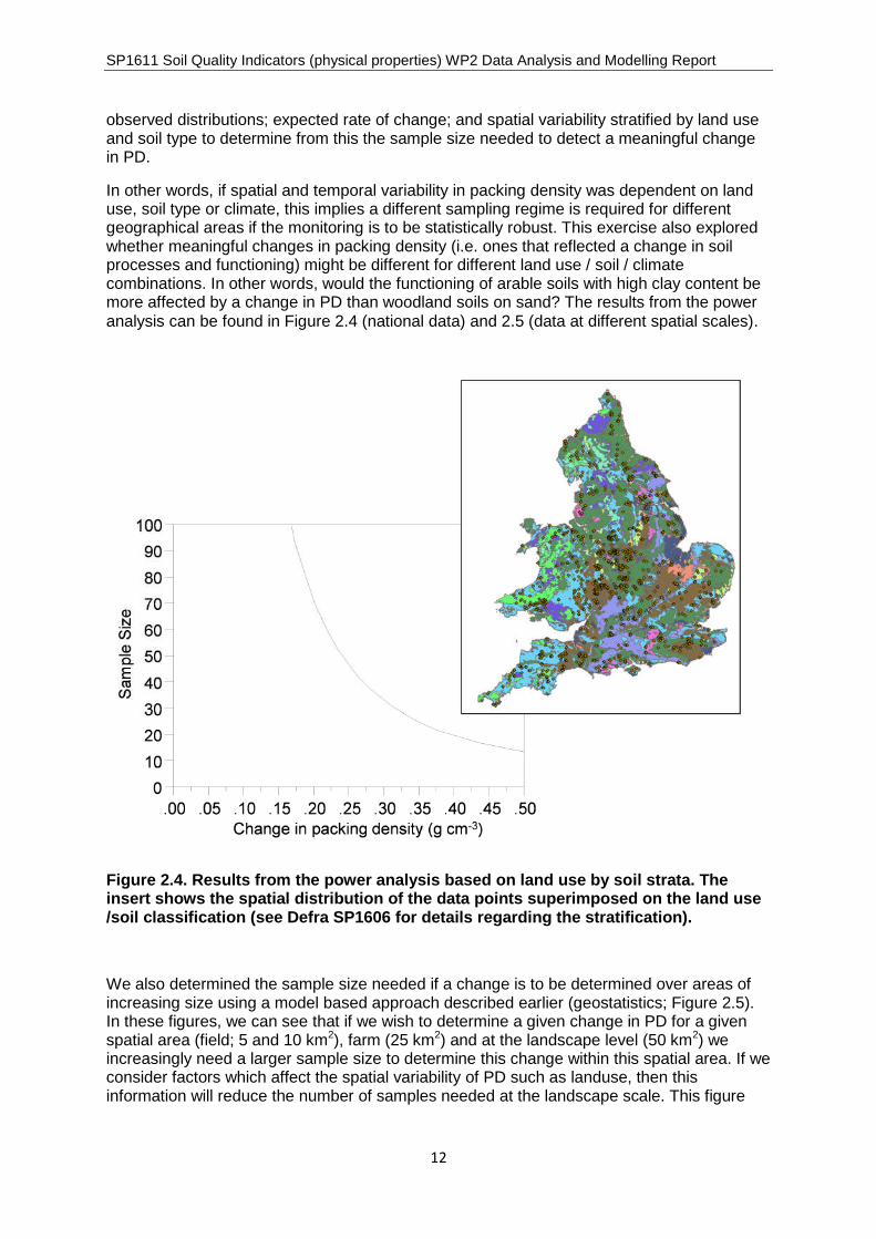
observed distributions; expected rate of change; and spatial variability stratified by land useand soil type to determine from this the sample size needed to detect a meaningful changein PD.
In other words, if spatial and temporal variability in packing density was dependent on landuse, soil type or climate, this implies a different sampling regime is required for differentgeographical areas if the monitoring is to be statistically robust. This exercise also exploredwhether meaningful changes in packing density (i.e. ones that reflected a change in soilprocesses and functioning) might be different for different land use / soil / climatecombinations. In other words, would the functioning of arable soils with high clay content bemore affected by a change in PD than woodland soils on sand? The results from the poweranalysis can be found in Figure 2.4 (national data) and 2.5 (data at different spatial scales).
Figure 2.4. Results from the power analysis based on land use by soil strata. Theinsert shows the spatial distribution of the data points superimposed on the land use/soil classification (see Defra SP1606 for details regarding the stratification).
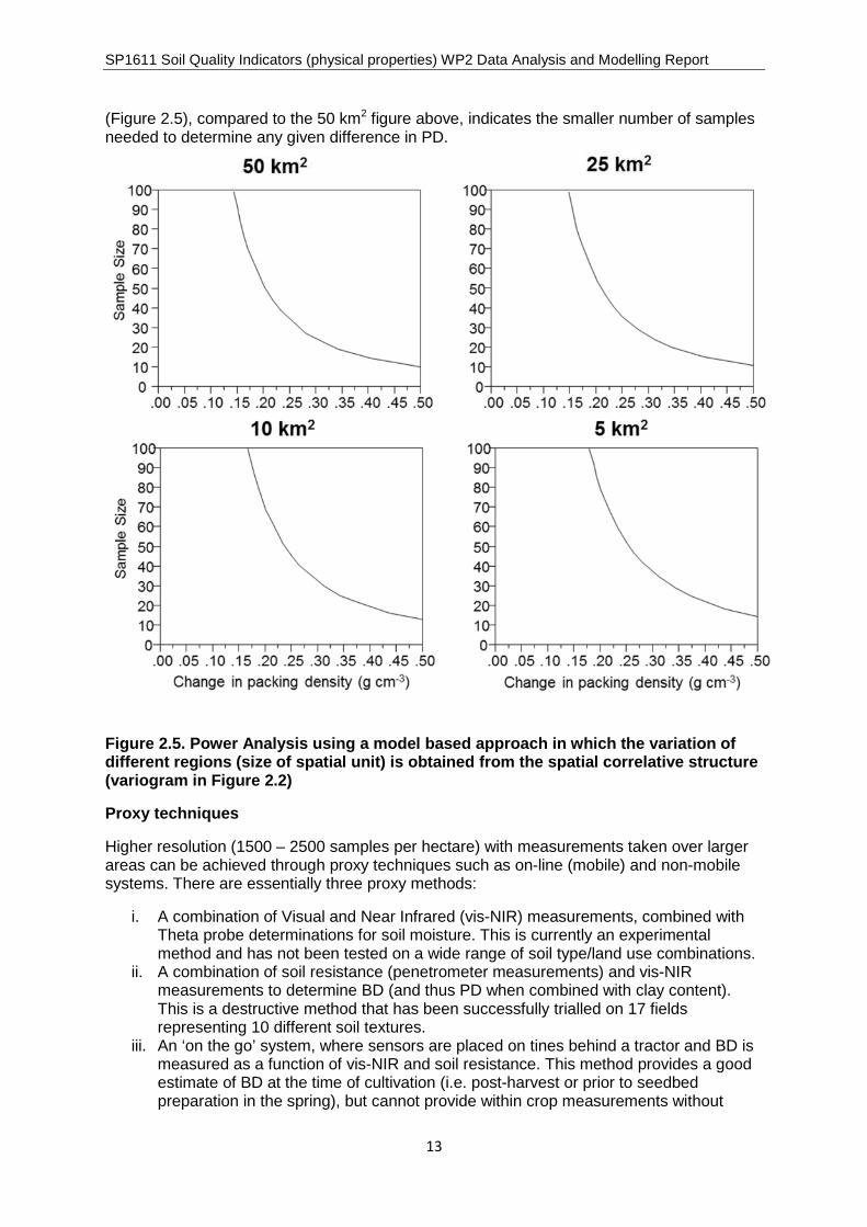
We also determined the sample size needed if a change is to be determined over areas ofincreasing size using a model based approach described earlier (geostatistics; Figure 2.5).In these figures, we can see that if we wish to determine a given change in PD for a givenspatial area (field; 5 and 10 km2), farm (25 km2) and at the landscape level (50 km2) weincreasingly need a larger sample size to determine this change within this spatial area. If weconsider factors which affect the spatial variability of PD such as landuse, then thisinformation will reduce the number of samples needed at the landscape scale. This figure
SP1611 Soil Quality Indicators (physical properties) WP2 Data Analysis and Modelling Report
13
(Figure 2.5), compared to the 50 km2 figure above, indicates the smaller number of samplesneeded to determine any given difference in PD.
Figure 2.5. Power Analysis using a model based approach in which the variation ofdifferent regions (size of spatial unit) is obtained from the spatial correlative structure(variogram in Figure 2.2)
Proxy techniques
Higher resolution (1500 – 2500 samples per hectare) with measurements taken over largerareas can be achieved through proxy techniques such as on-line (mobile) and non-mobilesystems. There are essentially three proxy methods:
i. A combination of Visual and Near Infrared (vis-NIR) measurements, combined withTheta probe determinations for soil moisture. This is currently an experimentalmethod and has not been tested on a wide range of soil type/land use combinations.
ii. A combination of soil resistance (penetrometer measurements) and vis-NIRmeasurements to determine BD (and thus PD when combined with clay content).This is a destructive method that has been successfully trialled on 17 fieldsrepresenting 10 different soil textures.
iii. An ‘on the go’ system, where sensors are placed on tines behind a tractor and BD ismeasured as a function of vis-NIR and soil resistance. This method provides a goodestimate of BD at the time of cultivation (i.e. post-harvest or prior to seedbedpreparation in the spring), but cannot provide within crop measurements without

SP1611 Soil Quality Indicators (physical properties) WP2 Data Analysis and Modelling Report
14
causing some crop damage. The system has been trialled in most soil texture typesin the UK.
All three methods involve multiple sensors and advanced data fusion techniques (Mouazenand Ramon, 2006).

SP1611 Soil Quality Indicators (physical properties) WP2 Data Analysis and Modelling Report
15
2.6 Fact Sheet 2. Soil Water Retention Characteristics.
Background
A series of important physical SQIs can be derived directly from soil water retentioncharacteristics. These SQIs, sometimes referred to as capacity-based indicators, includeplant available water capacity (PAWC), air capacity (AC; or drainable porosity), relative fieldcapacity (RFC), macroporosity (M), porosity of the soil matrix (e.g. Reynolds et al., 2002;2009) and the soil physical quality index S, developed by Dexter (2004a,b,c).
An important feature of these physical SQIs is that they are related to both pore volume andpore size distribution (Reynolds et al., 2009). As such, and as with hydraulic parameters ingeneral, these indicators, including S, are likely to be more sensitive to temporal and spatialchanges in soil condition and quality than other indicators which are governed by porevolume alone (e.g. bulk density) (Dexter, 2004a; Merrington et al 2006).
Soil physical quality index S
S is defined as the modulus of the slope of the soil water release function (plotted againstthe natural logarithm of the matric potential or pressure head) at its inflection point. The soilwater release function used is the Van Genuchten equation (1980) which is fitted to waterrelease curve data:
= −) +ቈ( ൬
∝ ൰
+ (1)
Where θ is the moisture content, h is the pressure head, θsat is the saturated moisturecontent, θres (residual moisture content) α and n are fitting parameters and m = 1 – 1/n.
Following Dexter (2004a), the water retention function (Eq. 1) is subsequently differentiatedwith respect to the natural logarithm of the pressure head, h, to give an indication of the poresize distribution, maximum pore size and frequency of pores in this maximum pore class:
()ܖܔ= − −) +]ࢻ( (∝ [(
(2)
Plotting the change in moisture content against the natural logarithm of the pressure headrather than pressure, h, is suggested to be a more appropriate measure of air entry intogranular material such as soil with a broad pore size distribution (Dexter and Bird, 2001).The inflection point of the water release curve, which is located at the peak of thedifferentiated function, is the point at which drainage is maximum and has two features, itslocation and its slope. The location is given by the pressure hi and according to Dexter(2004a) this occurs at:
=
∝
൨
(3)
with a corresponding water content, θi:
= −) +(
൨
+ (4)
According to Dexter (2004a), the slope of the curve at this point, S, is the modulus of:
SP1611 Soil Quality Indicators (physical properties) WP2 Data Analysis and Modelling Report
16
= ቤ)− ( +
൨(ା )
ቤ(5)
Note that if the gravimetric water content is used to plot the curve (as originally done byDexter (2004a)) instead of the volumetric water content, two different indices (Sg and Sv,respectively) are obtained. They are however related through the soil dry bulk density, ρb, sothat:
= (6)
The inflection point of the water release curve occurs at the matric potential, hi,representative of the dominant pore size of the soil where the specific water capacity ishighest. Hence, the S value can be considered as an overall index of physical and structuralquality in managed soils (Dexter, 2004a; Reynolds et al., 2009). The S index derived fromsoil hydraulic behaviour has been related to other soil physical processes by Dexter and co-workers (Dexter, 2004a, b, c; Gate et al., 2006; Dexter and Czyz, 2007; Dexter and Richard,2009) and correlated to other soil quality indicators such as bulk density and organic mattercontent. Dexter (2004a) also showed that the S index was related to the root growth of soil.
Relationship to soil functions
The higher the value of S, the higher the soil physical quality. Dexter (2004a) providedcategories of physical quality which classed soils with an Sg value of ≥ 0.035 as having ‘good’ physical quality and those with Sg ≥ 0.050 as having ‘very good’ physical quality. The maximum value of Sg found by Dexter and Czyz (2007) was 0.140 and the majority ofagricultural soils studied had values of Sg which fell between 0.015 and 0.060. However,whilst Dexter (2004a) illustrates the widespread applicability of the physical quality index Sfor a range of agricultural soils, optimum ranges for other land uses have yet to bedeveloped.
Sands with unimodal and narrow pore size distributions will be characterised by a large Sindex, despite having poor structure and poor water or air capacity, for example. As such,Reynolds et al. (2009) suggest that the quality index S should be used in combination withother physical quality parameters, especially the other capacity-based indicators: plantavailable water capacity (PAWC); relative field capacity (RFC); and macroporosity (M). Inturn, these can be derived using key features of the water release curve:
the volumetric moisture content (cm3.cm-3) at field capacity, θfc, occurring at 0.5 or 1m (5or 10 kPa) pressure head;
the saturated moisture content, θsat, at 0m pressure head; the moisture content at permanent wilting point, θpwp, occurring at 150m pressure head;
and the porosity of the soil matrix, θm, occurring at 0.1m pressure head. The ranges of
optimal values for these indicators are reviewed below.
Plant Available Water Capacity (PAWC). Plant Available Water Capacity (vol / vol; cm3.cm-3)is an indicator of the soil's capacity to store and provide water that is available to plant roots.It is defined as PAWC = θFC - θPWP. This simply assumes that, above field capacity, the soildrains readily and that water is lost through percolation and that, below permanent wiltingpoint, plant roots are not able to extract water. The review by Reynolds et al. (2009)suggests that PAWC ≥ 0.20 is required for maximal root growth and function (Cockroft and Olsson, 1997), while 0.15 ≤ PAWC ≤ 0.20 is ‘good’, 0.10 ≤ PAWC ≤ 0.15 is ‘limited’, and PAWC ≤ 0.10 is ‘poor’ for root development. These values could be assumed to represent a

SP1611 Soil Quality Indicators (physical properties) WP2 Data Analysis and Modelling Report
17
meaningful change in this physical SQI as changes of this magnitude are expected to affectroot (and therefore crop) growth.
Macroporosity M. Macroporosity (cm3.cm-3) can be defined as M = θsat - θm which representsthe volume of macropores with an equivalent pore diameter ≥ 300 μm. It is an indicator of the capacity of the soil to quickly drain excess water and facilitate root growth (Reynolds etal., 2009). It can also potentially indicate good structure. According to Reynolds et al. (2009),M ≥ 0.05–0.10 is often considered optimal and M ≤ 0.04 has been found in soils degraded by compaction. Reynolds et al. (2009) propose M ≥ 0.07 as an optimal figure and M = 0.04 as a lower critical limit.
Relative Field Capacity RFC. Relative Field Capacity is defined as RFC = θFC / θsat and is anindicator of the capacity of the soil to store both water and air, relative to the total porevolume. RFC represents the proportion of pores filled with water at field capacity andtherefore informs directly on whether the soil tends to be too wet or too dry. Moisture contentat field capacity, θfc, on its own does not provide this information, unless it is associated withθsat or θpwp as with the indicators AC and PAWC. According to Reynolds et al (2009), for rain-fed agriculture and mineral soils, the optimal balance between available water and aircapacity occurs between 0.6 ≤ RFC ≤ 0.7. Values outside this range indicate insufficient water (≤ 0.6) or air (≥ 0.7) and a potential reduction in microbial activity, notably microbial production of nitrate, which can impact crop growth and yield. Again, these values could beassumed to represent a meaningful change in this physical SQI as changes of thismagnitude are expected to affect root (and therefore crop) growth.
Larger spatial scale effects
To be meaningful SQIs, the soil water retention characteristics listed above should beindicative of soil functions that operate at a large spatial scale (e.g. the water regulationfunction), beyond the laboratory scale where these relationships are often founded.Degradation of physical soil quality associated with agricultural land management affectshydrological response at field and small catchment scales (e.g. O’ Connell et al. 2004a,O’Connell et al., 2007; McIntyre and Marshall 2010). However, after reviewing the scientificliterature, O’Connell et al. (2004a) concluded that, although there was substantial evidenceof changes in land use and management practices affecting runoff generation at the localand small catchment scale, there was very limited evidence that these local changes werepropagated downstream at the larger catchment scale. Clearly there is a significantevidence gap in connecting soil hydrological processes (and how these are reflecting in soilphysical properties) at different spatial scales (i.e. laboratory to field to catchment)
O’Connell et al. (2007) and Beven et al. (2008) state that this is because of a combination ofuncertainty in estimates of precipitation inputs to a catchment; the nonlinear impacts ofchanging catchment inputs over time on stream discharges; the uncertainty inmeasurements of stream discharges (particularly during flood events); the uncertainty incharacterising land use / management patterns in space and time; and that significantimpacts at the small scale may not necessarily have significant impact at catchment scales,due to landscape connectivity. However, Beven et al. (2008) concluded that the difficulty inidentifying consistent change in soil hydrological processes given the limitations of theavailable data did not mean that change is not happening and should not be taken to imply apolicy of doing nothing.
In summary, whilst additional field to small catchment scale experimental research andmonitoring and modelling studies have been conducted since the previous reviews ofFD2114 (O’ Connell et al. 2004) and FD2120 (Beven et al., 2008)), no studies havecontradicted the conclusion of FD2120 that the variability between years and inconsistenciesin rainfall and flow data appear to dominate any impacts of land use and management

SP1611 Soil Quality Indicators (physical properties) WP2 Data Analysis and Modelling Report
18
change (and any effect these might have on soil physical properties such as soil waterretention characteristics) on flow characteristics at the catchment scale over time.
Sampling effort needed
This WP considers four aspects of each SQI: the uncertainty in measurement; the variabilityin the indicator; the expected rate of change in the indicator; and the spatial variabilityassociated with the indicator. These factors will determine the sampling effort needed todetect a change in the SQI.
The standard Soil Survey of England and Wale sampling method for determining soil waterretention characteristic is to collect three undisturbed soil samples per soil horizon (Averyand Bascomb, 1982). The samples are collected using a coring device that reduces samplecompaction. Samples are ideally collected in winter or spring when the soil is near fieldcapacity so that swelling clay soils are at their maximum expansion. The laboratorymeasurement for soil water retention can take several months depending on soil texture andthe number of observation points on the soil moisture release cure that are to be determined.For example, the initial saturation of the soil samples can take between 1 to 2 days for sandysoils and up to 2 weeks for clayey soils. Samples are then placed on tension tables andallowed to equilibrate to the tension (or suction) applied through the tension table.
Equilibration is determined by weighing the sample every 2 days until their weight change is<100 mg between weighing. For suctions >0.5m head of water (5kPa), the samples aretransferred to a pressure membrane apparatus where air pressure is used to force water outof the sample. Water is collected in a reservoir and weighed. When the weight of water <3mg per day over several days the samples are assumed to be equilibrated. The sample canthen be removed and weighted. Finally the sample is oven dried at 105oC to determine bulkdensity of the sample. The volumetric water content at each suction/pressure point can thenbe determined.
The soil water release characteristics are influenced by land use and soil management, andthese changes can occur over short time scales. It is generally accepted that soilhydrological properties to which soil water release characteristics are related, exhibit bothshort and long range variability (Nielsen et al., 1973). Samples that are collected closetogether (within a few meters) are more similar than those collected at greater distances.
Proxy techniques
Obtaining soil water retention curves to derive indicators such as the Dexter’s S is timeconsuming and requires considerable effort. Alternatively, pedotransfer functions (PTFs) canbe used to derive these properties from simple to measure soil characteristics. PTFs are(linear) relationships between the desired, but expensive to obtain soil properties (i.e. Sindex, AC, PAWC and RFC) and easily measured soil properties of which BD and soil C arethe most commonly used (Mayr and Jarvis 1999; Matula et al., 2007). In this case, given theeffort needed to obtain Soil Water Retention Characteristics, these SQIs can only beconsidered if it is feasible to develop a set of PTF’s from which these particular SQIs can bederived. We explore the feasibility of developing such PTF’s in the following section.
Determination of Soil Water Retention Characteristics (index S, AC, PAWC and RFC) fromthe LandIS data base
A total of 2480 soil profiles for which soil water retention data were available were extractedfrom the LandIS database. The relevant data available consisted of volumetric moisturecontent measured at pressure heads (expressed in water height equivalents) of 0.5, 1, 4, 20and 150 m. In addition, total porosity (derived from measured bulk density and particle

SP1611 Soil Quality Indicators (physical properties) WP2 Data Analysis and Modelling Report
19
density) was used as an approximation of the moisture content at saturation, θsat (= 0mpressure head). For each soil, the water retention function represented by the VanGenuchten equation (Eq 1) was fitted to the data using θres, α and n as fitting parameters. The Dexter’s S index was calculated with Eq 5, using the fitted parameters and convertedinto Sg using Eq. 6. θsat, estimated from the porosity, θfc (measured at both 0.5 and 1mpressure head) and θPWP (measured at 150m pressure head) were used to calculate theindicators AC, PAWC and RFC as described above (Table 2.4). It was not possible tocalculate macroporosity (M) because measurements of the moisture content, θm (occurringat 0.1m pressure head) were not given.
Assessment of pedotransfer functions
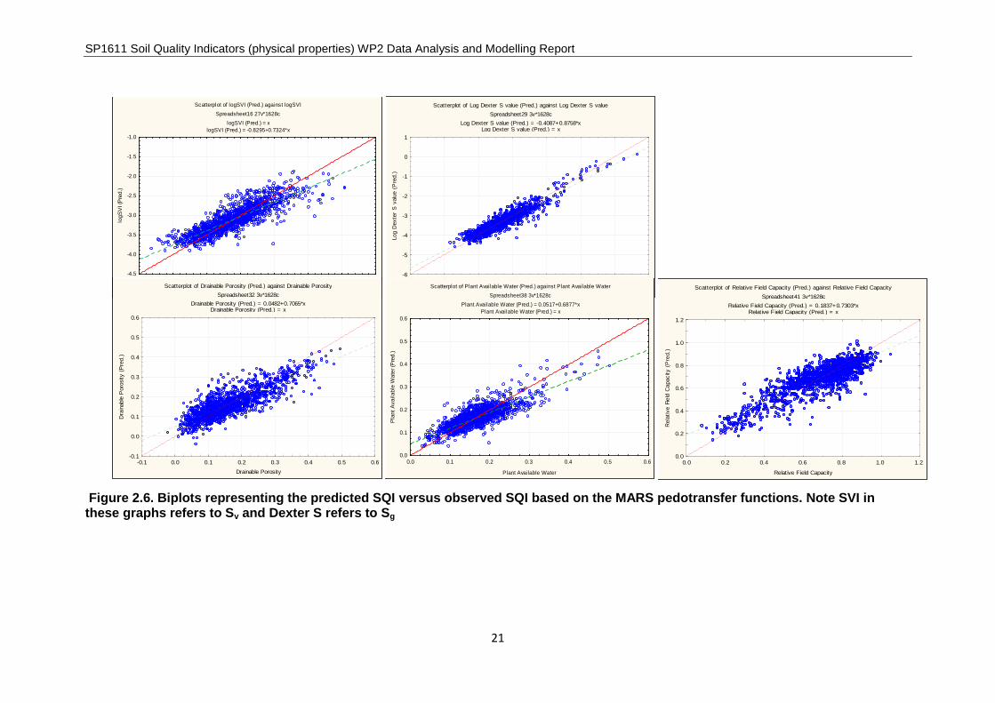
BD, texture (clay, silt and sand content) and organic C content are also available for thesame soils in the LandIS database. Two types of PTFs were considered (Figure 2.6): Thefirst represents the standard type PTF and is derived using multiple linear regressions(MLRs). The format of MLR models is:
= + ଵ ଵ + ଶଶ+. . . + ௫௫ + ܧ (7)
where Y is the dependent variable; a is a constant; bi are coefficients; Xi are predictorvariables; and E is an error term. To assess the predictive power of the model, a 10-foldcross validation was implemented using the DAAG package (Maindonald & Braun, 2011).The significant variables were chosen by a stepwise selection procedure using the stepAICfunction of the MASS package in R (Venables & Ripley, 2002).
The second PTF approach is an extension of MLR model, which can also considercategorical data such as ‘Soil Series’ and ‘Land use’ (Table 2.5). Multiple AdditiveRegression Splines (MARS splines) is a nonparametric regression technique that combinesboth regression splines and model selection methods (Friedman, 1991). It constructs a setspline basis functions (nonlinear functions) that are entirely determined from the regressiondata, and determines where they are applicable by automatically selecting appropriate knotvalues for different variables (in essence a multiple piecewise linear regression, where eachbreakpoint (or knot value) defines the "region of application" for a particular linear regressionequation).
Table 2.4. Soil Water Retention Characteristics: Fit results from PTFs based onLandIS data (BD, Clay, Silt and Sand and Organic C content)
Sv Sg
DrainablePorosity
PlantAvailable
WaterRelative Field
Capacity
RSQ concR
RSQ concR
RSQ concR
RSQ concR
RSQ concR
multipleregression
0.56 0.73 0.82 0.85 0.53 0.65 0.58 0.72 0.61 0.78
MARSsplines
0.72 0.75 0.87 0.9 0.71 0.08 0.68 0.82 0.73 0.85
RSQ = R2 statistic; conc R = concordance correlation
Table 2.5. Variable importance in MARS fitting. Numbers refer to rankings ofimportance

SP1611 Soil Quality Indicators (physical properties) WP2 Data Analysis and Modelling Report
20
Sv Sg DrainablePorosity
PlantAvailable
Water
RelativeField
Capacity
BULKD 2 2 2 2 2
CLAY 3 2 2 2 1
SILT 0 1 0 2 2
SAND 1 2 2 2 2
ORGANIC_CARBON 1 2 1 3 1
LU_GROUP 0 0 0 0 0
SUBGROUP 1 1 4 1 3
SERIES 4 4 2 3 2
In summary, we can obtain adequate performance (R2 of 0.5 to 06) if we use standardregression approaches. This is significantly improved with MARS regression approachesusing data which are available for England and Wales (R2 > 0.8). It is therefore feasible toderive Soil Water Retention Characteristics SQIs using PTFs based on bulk density, textureand organic C measurements. In SP1305 (Subproject B), the sampling requirement, underdifferent sampling regimes, is considered for BD and organic C, and the report suggests thatfor a plot of 20 by 20 m, 25 aggregated samples would be required. This is indicative of thesampling effort needed to determine the input data for the PTFs.
SP1611 Soil Quality Indicators (physical properties) WP2 Data Analysis and Modelling Report
21
Figure 2.6. Biplots representing the predicted SQI versus observed SQI based on the MARS pedotransfer functions. Note SVI inthese graphs refers to Sv and Dexter S refers to Sg
Scatterplot of logSVI (Pred.) against logSVI
Spreadsheet16 27v*1628c
logSVI (Pred.) = x
logSVI (Pred.) = -0.8295+0.7324*x
-4.5 -4.0 -3.5 -3.0 -2.5 -2.0 -1.5 -1.0
logSVI
-4.5
-4.0
-3.5
-3.0
-2.5
-2.0
-1.5
-1.0
logS
VI(P
red.)
Scatterplot of Log Dexter S value (Pred.) against Log Dexter S value
Spreadsheet29 3v*1628c
Log Dexter S value (Pred.) = -0.4087+0.8758*xLog Dexter S value (Pred.) = x
-6 -5 -4 -3 -2 -1 0 1
Log Dexter S value
-6
-5
-4
-3
-2
-1
0
1
Log
Dexte
rS
valu
e(P
red.)
Scatterplot of Drainable Porosity (Pred.) against Drainable Porosity
Spreadsheet32 3v*1628c
Drainable Porosity (Pred.) = 0.0482+0.7065*xDrainable Porosity (Pred.) = x
-0.1 0.0 0.1 0.2 0.3 0.4 0.5 0.6
Drainable Porosity
-0.1
0.0
0.1
0.2
0.3
0.4
0.5
0.6
Dra
inable
Poro
sity
(Pre
d.)
Scatterplot of Plant Available Water (Pred.) against Plant Available Water
Spreadsheet38 3v*1628c
Plant Available Water (Pred.) = 0.0517+0.6877*x
Plant Available Water (Pred.) = x
0.0 0.1 0.2 0.3 0.4 0.5 0.6
Plant Available Water
0.0
0.1
0.2
0.3
0.4
0.5
0.6
Pla
ntA
vailable
Wate
r(P
red.)
Scatterplot of Relative Field Capacity (Pred.) against Relative Field Capacity
Spreadsheet41 3v*1628c
Relative Field Capacity (Pred.) = 0.1837+0.7303*xRelative Field Capacity (Pred.) = x
0.0 0.2 0.4 0.6 0.8 1.0 1.2
Relative Field Capacity
0.0
0.2
0.4
0.6
0.8
1.0
1.2
Rela
tive
Fie
ldC
apacity
(Pre
d.)

SP1611 Soil Quality Indicators (physical properties) WP2 Data Analysis and Modelling Report
22
2.7 Fact Sheet 3. Aggregate Stability
Background
Aggregate stability is a measure of the resistance of a soil to the destructive effects ofrainfall, runoff and wind. The four main mechanisms responsible for surface soil aggregatebreakdown by water are: (i) slaking, (ii) differential swelling, (iii) mechanical breakdown byraindrop impact and (iv) physico-chemical dispersion (Le Bissonnais, 1996). The breakdownof aggregates and reorientation of resulting fragments on the soil surface leads to surfacecrust formation, with higher bulk densities, restricted infiltration and greater runoff / erosionhazard. Aggregate stability is an integrative indicator in that it reflects physical, biological andchemical soil properties. Aggregate stability is also multi-faceted as it reflects both soilfunctioning capacity (e.g. water regulation via infiltration rate) and susceptibility todegradation (e.g. soil erosion). Stable aggregates maintain soil structure in terms of a rangeof pore sizes, and thus promote soil aeration, water infiltration, drainage, better workability,seed bed quality and root penetration. More stable aggregates, with a higher proportion oflarge to small aggregates, suggest better soil quality, although this is unlikely to be a linearrelationship. The stability of aggregates can be inferred by measurements of aggregatestability (Saygin et al., 2012).
To investigate the uncertainty in measurement; variability in observed distributions; expectedrate of change; and spatial variability, we found only very limited datasets to assessaggregate stability across different land uses and soils at the national scale (England andWales) (Thompson and Peccol, 1995; Merrington et al., 2006). However, Defra projectSP0519 (Critical levels of soil organic carbon in surface soils in relation to soil stability,function and infiltration) used measurements of aggregate stability to describe and rank thelikely behaviour of soil under the influence of rain. A number of simple aggregate stabilitytests were designed to allow rapid screening of a relatively large number of representativesoil type / land use combinations in terms of their susceptibility to aggregate breakdown.General relationships between aggregate stability and measurements of a wide range of keyphysical and chemical soil properties were deduced, including easily-measurable soilproperties such as organic carbon and clay content. The resultant database has been madeavailable to the current project by Dr. Chris Watts and Prof. Andy Whitmore of BBSRCRothamsted Research. However, as the authors of that work point out, the data generatedfrom the field experiments is limited, in terms of geographical distribution, environmentalconditions, simulated plot scale and replication.
Relationship to soil functions
Aggregate breakdown and subsequent aggregate size distribution affect soil processes andfunctions through their effect on:
i) Biomass production (provisioning function; Figure 2.7). Surface sealing by dislodged soilparticles resulting from aggregate breakdown affects crop emergence. Surface sealsalso reduce infiltration capacity / hydraulic conductivity, so affecting soil moisturecontent, and availability of plant nutrients and water to roots. Some studies have relatedcrop yields to aggregate stability (e.g. Skukla et al., 2004; Figure 2.7), but furtheranalysis was not possible here, due to lack of data for England and Wales..

SP1611 Soil Quality Indicators (physical properties) WP2 Data Analysis and Modelling Report
23
Figure 2.7. Relationships between production function (yield grain) and aggregatestability (Skukla et al., 2004)
ii) Regulation of water and carbon: surface sealing resulting from aggregate breakdownaffects infiltration/hydraulic conductivity through soil. Carbon regulation and sequestrationare affected due to mineralization and loss of C on aggregate breakdown.
We considered this relationship as data in the Defra project SP0519 (Critical levels of soilorganic carbon in surface soils in relation to soil stability, function and infiltration) containedmeasures of aggregate stability and the runoff observed in these experiments. In Figure2.8a, we represent the observed relationship between aggregate stability (as measured bythe 3 different methods used) and surface runoff. These data show only very weak or norelationship between aggregate stability and runoff generated; therefore currently there is noevidence that aggregate stability is an effective SQI of the water regulation function.
iii) Resistance to degradation – aggregate stability is strongly related to erosion susceptibility(it is regarded as the best estimator of erodibility/soil susceptibility to erosion (Bryan,1968)), soil compaction and loss of C (Stavi et al., 2011). It also determines the degree ofand susceptibility to soil surface sealing and capping.
Using data from the Defra project SP0519 (Critical levels of soil organic carbon in surfacesoils in relation to soil stability, function and infiltration) we analysed the relationshipsbetween aggregate stability and soil losses under simulated rainfall in the laboratory and inthe field (Figure 2.8b). The soil loss results of the field work and laboratory trials were incontrast with those obtained using the three methods of aggregate stability determination,which used highly disturbed beds of aggregates.
Sampling effort needed
Usually individual aggregates are tested, although groups of aggregates can be tested undersimulated rainfall. One major challenge is extrapolating results from the individual aggregatescale to larger spatial scales at which related soil processes (e.g. infiltration, erosion) andsoil functions (e.g. provisioning) take place. For example, when relating aggregate stability tothrough flow (infiltration) and erosion, we found no clear relationships using the DefraSP0519 data (Figure 2.8b and 2.8c)
The high variability in aggregate stability as reported in the literature suggests a very highsampling intensity is required to detect changes in space and time. Aggregate stability isbiologically mediated, so is likely to change during the growing season but there is onlylimited scientific literature on this.

SP1611 Soil Quality Indicators (physical properties) WP2 Data Analysis and Modelling Report
24
0.8 1.0 1.2 1.4 1.6 1.8 2.0 2.2 2.4 2.6 2.8 3.0 3.2 3.4
AS mechanical (mm)
0
10
20
30
40
50
60
70
80
90A
v%
runoff
r2 = 0.0007
1.8 2.0 2.2 2.4 2.6 2.8 3.0 3.2 3.4 3.6
AS slow (mm)
0
10
20
30
40
50
60
70
80
90
Av
%ru
noff
r2 = 0.2416
0.6 0.8 1.0 1.2 1.4 1.6 1.8 2.0 2.2 2.4 2.6 2.8 3.0 3.2
AS fast (mm)
0
10
20
30
40
50
60
70
80
90
Av
%ru
noff
r2 = 0.0004
Figure 2.8a. Biplot and linear fit between % Runoff and aggregate stability. Data fromDefra project SP0519 (Critical levels of soil organic carbon in surface soils in relationto soil stability, function and infiltration). Experimental details can be found in theproject report.
Power analysis and sampling size.
For aggregate stability, we base the power analysis on data obtained in the Defra projectSP0519 in which particular aggregate fractions were associated with degrees of stability(very unstable, unstable, medium, stable, very stable). Three types of aggregate stability testwere considered using various wetting conditions and energies (fast wetting (AS fast); slowwetting (AS slow); and mechanical energy applied after pre-wetting (AS mechanical)). If weconsider the resulting degrees of stability as qualitative categories of aggregate stability(Table 2.6), then we can base the power analysis on the differences between thesecategories (Figure 2.9)

SP1611 Soil Quality Indicators (physical properties) WP2 Data Analysis and Modelling Report
25
0.8 1.0 1.2 1.4 1.6 1.8 2.0 2.2 2.4 2.6 2.8 3.0 3.2 3.4
AS mechanical (mm)
-4
-3
-2
-1
0
1
2
Tota
lSedim
entE
roded
log(g
)
r2 = 0.1909
0.6 0.8 1.0 1.2 1.4 1.6 1.8 2.0 2.2 2.4 2.6 2.8 3.0 3.2
AS fast (mm)
-4
-3
-2
-1
0
1
2
Tota
lSedim
entE
roded
log(g
)
r2 = 0.1981
1.8 2.0 2.2 2.4 2.6 2.8 3.0 3.2 3.4 3.6
AS slow (mm)
-4
-3
-2
-1
0
1
2
Tota
lSedim
entE
roded
log(g
)
r2 = 0.4327
0.6 0.8 1.0 1.2 1.4 1.6 1.8 2.0 2.2 2.4 2.6 2.8 3.0 3.2
AS fast (mm)
0
10
20
30
40
50
60
70
80
90
Av
%th
roflo
w
r2 = 0.0421
1.8 2.0 2.2 2.4 2.6 2.8 3.0 3.2 3.4 3.6
AS slow (mm)
0
10
20
30
40
50
60
70
80
90
Av
%th
roflo
w
r2 = 0.0711
0.8 1.0 1.2 1.4 1.6 1.8 2.0 2.2 2.4 2.6 2.8 3.0 3.2 3.4
AS mechanical (mm)
0
10
20
30
40
50
60
70
80
90
Av
%th
roflo
w
r2 = 0.0887
Figure 2.8b Biplot and linear fit between %through flow and aggregate stability. Datafrom Defra project SP0519 (Critical levels ofsoil organic carbon in surface soils inrelation to soil stability, function andinfiltration). Experimental details can befound in the project report.
Figure 2.8c Biplot and linear fit between totalsediment eroded and aggregate stability. Datafrom Defra project SP0519 (Critical levels ofsoil organic carbon in surface soils in relationto soil stability, function and infiltration).

SP1611 Soil Quality Indicators (physical properties) WP2 Data Analysis and Modelling Report
26
Experimental details can be found in the project report.Table 2.6. Classification of aggregate stability based on mean weight diameter (MWD;after Le Bissonnais, 1996)MWD 0.4 mm Very UnstableMWD 0.4 - 0.8 mm UnstableMWD 0.8 - 1.3 mm MediumMWD 1.3 - 2.0 mm StableMWD >2.0 mm Very Stable
Figure 2.9 Power analysis of three different measurement techniques to determineaggregate stability. Data from Defra project SP0519 (Critical levels of soil organiccarbon in surface soils in relation to soil stability, function and infiltration).
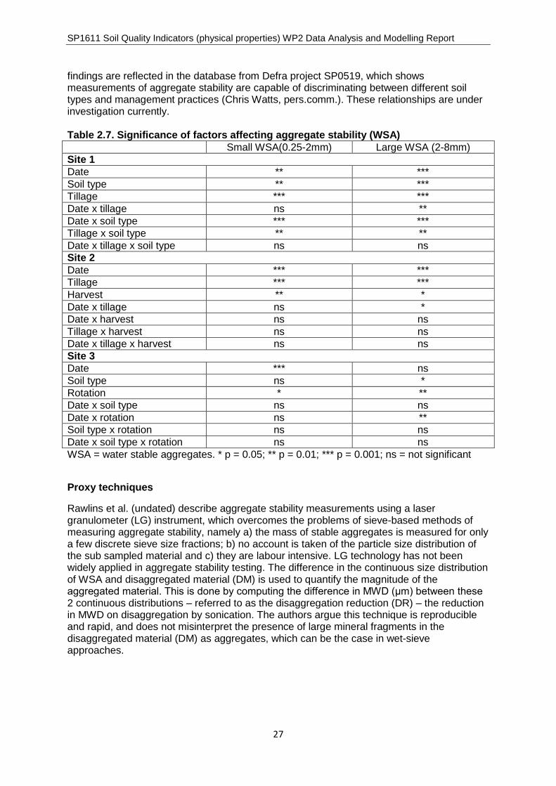
However, aggregate stability measurements cannot be used in isolation as meaningfulphysical SQIs, as results must be interpreted in conjunction with information on soil type,changes in land use and management and climate (as reported at the Technical Workshop,Science Project SC030265; Merrington et al., 2008). Indeed, the sensitivity of aggregatestability to different factors is shown in data from Moebius et al., (2007; Table 2.7). These
SP1611 Soil Quality Indicators (physical properties) WP2 Data Analysis and Modelling Report
27
findings are reflected in the database from Defra project SP0519, which showsmeasurements of aggregate stability are capable of discriminating between different soiltypes and management practices (Chris Watts, pers.comm.). These relationships are underinvestigation currently.
Table 2.7. Significance of factors affecting aggregate stability (WSA)Small WSA(0.25-2mm) Large WSA (2-8mm)
Site 1Date ** ***Soil type ** ***Tillage *** ***Date x tillage ns **Date x soil type *** ***Tillage x soil type ** **Date x tillage x soil type ns nsSite 2Date *** ***Tillage *** ***Harvest ** *Date x tillage ns *Date x harvest ns nsTillage x harvest ns nsDate x tillage x harvest ns nsSite 3Date *** nsSoil type ns *Rotation * **Date x soil type ns nsDate x rotation ns **Soil type x rotation ns nsDate x soil type x rotation ns nsWSA = water stable aggregates. * p = 0.05; ** p = 0.01; *** p = 0.001; ns = not significant
Proxy techniques
Rawlins et al. (undated) describe aggregate stability measurements using a lasergranulometer (LG) instrument, which overcomes the problems of sieve-based methods ofmeasuring aggregate stability, namely a) the mass of stable aggregates is measured for onlya few discrete sieve size fractions; b) no account is taken of the particle size distribution ofthe sub sampled material and c) they are labour intensive. LG technology has not beenwidely applied in aggregate stability testing. The difference in the continuous size distributionof WSA and disaggregated material (DM) is used to quantify the magnitude of theaggregated material. This is done by computing the difference in MWD (μm) between these 2 continuous distributions – referred to as the disaggregation reduction (DR) – the reductionin MWD on disaggregation by sonication. The authors argue this technique is reproducibleand rapid, and does not misinterpret the presence of large mineral fragments in thedisaggregated material (DM) as aggregates, which can be the case in wet-sieveapproaches.

SP1611 Soil Quality Indicators (physical properties) WP2 Data Analysis and Modelling Report
28
2.8 Fact Sheet 4. Rate of Erosion
Background
Soil erosion represents the physical loss of the soil resource, along with the functions(ecosystem goods & services) associated with that resource. This definition suggestserosion is a meaningful indictor of soil quality (Lal, 1998). Erosion is the detachment andtransport of soil particles / aggregates from the in-situ soil mass, leading to a reduction in soildepth and volume (assuming soil bulk density is constant). Soil erosion is measured as themass (tonnes) of soil lost per unit space (hectare) per unit time (year) (t ha-1 y-1). The changein the rate of erosion over space and time can also be monitored, although it is normallydifficult to split out temporal changes due to management from changes in erosion rate dueto changes in rainfall duration and intensity. Rates of soil erosion can be converted intodepth of eroded soil using the equation:
ܦ �ℎݐ ݏ� �ݏݏ� )�ݑ�ݎ ) = 0.1ܯ �ݏݏ ݏ� �ݏݏ� (ଵݕ��ℎଵݐ)�ݑ�ݎ
ݑܤ � �ݕݐݏ ℎݐ� ݏ� �ܯ)� ଷ)
e.g. 10 t ha-1 y-1 = 0.7mm depth of soil lost per annum = 70mm/ century, assuming a soilbulk density = 1.4 Mg m3.
To investigate the uncertainty in measurement; variability in observed distributions; expectedrate of change; and spatial variability, we reviewed possible data sources. Actual erosionrates are measured on field plots (associated with high levels of inter- and intra-plotvariability in space and time; Brazier et al., 2012); through volumetric surveys of rill and gullyfeatures (although operator error may occur and accuracy is related to the number ofreadings; Evans, 2002); and via remote sensing (ground, air and satellite imagery – issueshere relate to cost, frequency of image capture, resolution of images to capture erosionfeatures as reported in Brazier et al., 2012).Many monitoring schemes have concentrated on arable land and are biased as they tendedto only consider land susceptible to erosion. Sheet or interrill erosion (caused by non-concentrated overland flow) is usually not monitored, but this can contribute a significantproportion of soil loss on upper and middle slopes (Morgan, 2005). As such, previous studiesand the rates they measured are not representative of erosion rates on all soil / land usecombinations in England and Wales.
Brazier et al. (2012) considered the application of relatively innovative Cs137 techniques tosupply erosion monitoring data at the national scale (see Quine and Walling, 1991; Wallingand Quine, 1991). Using these techniques in Defra SP0411 (Walling et al., 2005) andSP0413 (Walling et al., 2008), erosion rate data were collated for 248 fields, providing abasis for assessing the range of erosion rates occurring on agricultural land in England andWales (Table 2.8). The data represent the first sizeable dataset of soil erosion rates foragricultural land in England and Wales that explicitly includes sheet erosion and includesvalues of both gross and net erosion.

SP1611 Soil Quality Indicators (physical properties) WP2 Data Analysis and Modelling Report
29
Table 2.8. Comparison of estimates of gross and net erosion rates obtained forindividual fields using the Cs137 technique with those obtained from moredetailed sampling involving multiple transects and grid sampling (From Walling etal., 2005)Location Land use Gross soil loss (t ha-1 y-1) Net soil loss (t ha-1 y-1)
Cs137technique
Intensivesampling
Cs137technique
Intensivesampling
Crediton Arable 6.2 7.1 0.7 0.6Yeovil Arable 9.7 8.7 5.7 6.3Yeovil Grass 2.1 1.7 0.2 0.2Cadeleigh Grass 0.6 0.4 0 0Crediton Arable 8.3 9.1 3.6 4.4Cadeleigh Arable 6.2 5.4 0.5 0.8
Given the data reported in the literature, we need to relate these rates of erosion with effectson soil processes and thus soil functions.
Relationship to soil functions
All soil functions are degraded by erosion due to the complete loss of soil profile. Productionfunctions are affected by loss of soil depth / volume (see 2.9 Depth of Soil Indicator) and theinconvenience of erosion features interrupting farming operations. The regulation of waterand carbon are affected by erosion through impacts on soil infiltration, flood risk increase,water quality decline, irregularity of rivers flow and increase of sedimentation in waterbodies. Erosion causes perturbation of ecosystems and reduced ecological connectivitywhich both affect biodiversity and associated functions. As such, soil erosion indicates adegradation of soil quantity and quality (Huber et al., 2008). The impact of soil erosion onsoil function and associated economic costs are reviewed in Defra SP1606. Soil erosion cancause a detectable change in soil quality, depending on:
a) the rate of erosion – low rates have no / little effect if they occur at a tolerable ratedefined as “any mean annual cumulative (all erosion types combined) soil erosion rate atwhich a deterioration or loss of one or more soil functions does not occur” (Verheijen etal., 2009); and
b) inherent soil quality – some soils may not lose functioning as a result of erosion,depending on soil qualities such as soil depth, nutrient status and organic matter content(Lal, 1998). This can be captured in the concept of ‘soil loss tolerance’ (Verheijen et al.,2009)
These two points are captured in the concept of the life span of a soil. This is an extension ofthe idea of ‘tolerable soil loss’ and has been described as:
Tc = S / (E – P)
where, Tc is the critical life span of the soil, S is the initial soil thickness (m) of the A-horizon(see 2.9 Soil depth as an SQI below), E is the net soil erosion rate given by the differencebetween erosion and deposition (m yr-1), and P is the soil production rate (m yr-1;representing the provisioning function) (Bui et al., 2010). The life span of a soil is the timetaken to exhaust the soil below a point where it can no longer support production and occursas a result of tolerable soil loss being exceeded.
Tolerable soil erosion has been defined by Boardman and Poesen (2006) as the rate of soilerosion no larger than the rate of soil production. However, Verheijen et al. (2009) suggest,that a more appropriate definition of tolerable soil erosion should be more holistic in itsinclusion of soil functions and therefore should be ‘any actual soil erosion rate at which a

SP1611 Soil Quality Indicators (physical properties) WP2 Data Analysis and Modelling Report
30
deterioration or loss of one or more soil functions does not occur’, where actual soil erosionmeans the cumulative amount of soil lost by all recognised erosion types. The term ‘tolerablesoil erosion’ is preferable when referring to soil lost by erosion in the context of soilprotection because it includes the removal of soil material by both physical processes(erosion), and biochemical processes (solute/gaseous export of mineral matter anddecomposition of organic matter) (Verheijen et al., 2009). In Europe the tolerable soil erosionrate ranges from 0.3 to 1.4 t ha-1 yr-1.
Verheijen et al. (2009) estimate that based on soil formation and erosion rates and soilmanagement techniques at the time, topsoil in tilled arable land on hill slopes could be ca. 2to 30 cm thinner in 100 years’ time (assuming a tolerable rate of 1 t ha-1 yr-1 and a bulkdensity of 1.3 t m-3)
Erosion is both a dependent (e.g. OMC affects vulnerability of soil to erosion) andindependent (e.g. erosion affects OMC levels; Quinton et al., 2006; Defra SP0519) variablein soil quality assessment.
There are many factors affecting rate of erosion and the change in that rate. Thiscomplicates understanding of its responsiveness / sensitivity to a change in any one or acombination of these factors. In other words, there is poor discrimination in the signal.Erosion rates are highly variable due to the many factors affecting rate. These factors are:
i. Rainfall erosivity, which is based on intensity, duration and kinetic energy of rainfall.“Climate – more specifically the combination of soil antecedent moisture conditions,rainfall intensity and duration – is a dominant driver of soil erosion by water. Its variationwill lead to large differences in mean erosion rates between years for whichmeasurements are made.”
ii. Soil erodibility, which is correlated to aggregate stability, soil texture, OMC, infiltration /permeability, bulk density and structure, is known to affect gross erosion rates (Table2.10).
Table 2.10. Responsiveness of erosion rate to soil texture (From Walling et al., 2005)
Soil texture Number ofsites
Gross erosion rates ( t ha-1 year-1)
Median STD
Clay 8 4.2 2.6
Clay loam 26 7.7 2.5
Silt loam 13 12.8 4.5
Sandyloam
15 9.9 3.6
iii. Slope length, gradient, curvature and plan all affect erosion rate (Morgan, 2005).Several equations exist to represent slope characteristics and associated changes inerosion rate. However, Evans and Cook (1986) reported the lack of a clearrelationship between erosion rate and slope gradient in an analysis of rillerosion rates on agricultural fields (Figure 2.10).
iv. Land cover / land use (horticulture, arable, pasture, woodland, urban etc.) / landmanagement practices are significant factors in determining soil erosion rates
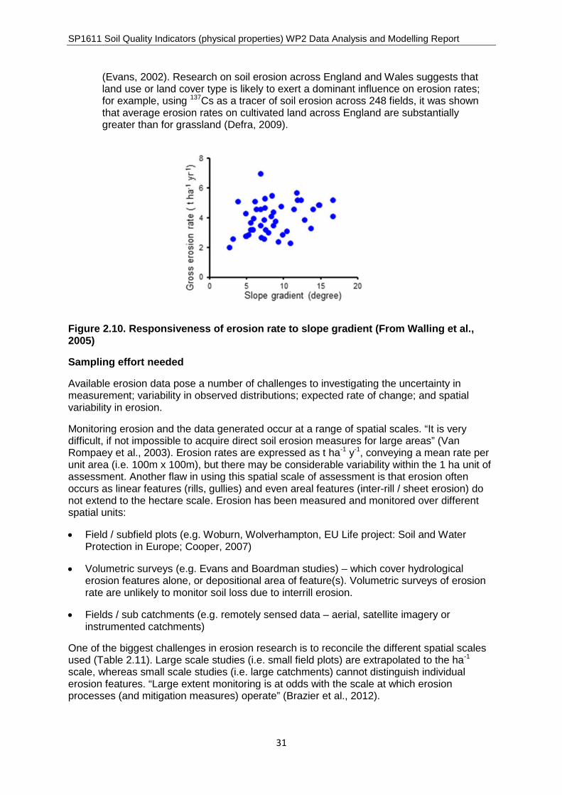
SP1611 Soil Quality Indicators (physical properties) WP2 Data Analysis and Modelling Report
31
(Evans, 2002). Research on soil erosion across England and Wales suggests thatland use or land cover type is likely to exert a dominant influence on erosion rates;for example, using 137Cs as a tracer of soil erosion across 248 fields, it was shownthat average erosion rates on cultivated land across England are substantiallygreater than for grassland (Defra, 2009).
Figure 2.10. Responsiveness of erosion rate to slope gradient (From Walling et al.,2005)
Sampling effort needed
Available erosion data pose a number of challenges to investigating the uncertainty inmeasurement; variability in observed distributions; expected rate of change; and spatialvariability in erosion.
Monitoring erosion and the data generated occur at a range of spatial scales. “It is verydifficult, if not impossible to acquire direct soil erosion measures for large areas” (VanRompaey et al., 2003). Erosion rates are expressed as t ha-1 y-1, conveying a mean rate perunit area (i.e. 100m x 100m), but there may be considerable variability within the 1 ha unit ofassessment. Another flaw in using this spatial scale of assessment is that erosion oftenoccurs as linear features (rills, gullies) and even areal features (inter-rill / sheet erosion) donot extend to the hectare scale. Erosion has been measured and monitored over differentspatial units:
Field / subfield plots (e.g. Woburn, Wolverhampton, EU Life project: Soil and WaterProtection in Europe; Cooper, 2007)
Volumetric surveys (e.g. Evans and Boardman studies) – which cover hydrologicalerosion features alone, or depositional area of feature(s). Volumetric surveys of erosionrate are unlikely to monitor soil loss due to interrill erosion.
Fields / sub catchments (e.g. remotely sensed data – aerial, satellite imagery orinstrumented catchments)
One of the biggest challenges in erosion research is to reconcile the different spatial scalesused (Table 2.11). Large scale studies (i.e. small field plots) are extrapolated to the ha-1
scale, whereas small scale studies (i.e. large catchments) cannot distinguish individualerosion features. “Large extent monitoring is at odds with the scale at which erosionprocesses (and mitigation measures) operate” (Brazier et al., 2012).
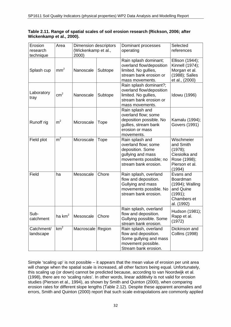
SP1611 Soil Quality Indicators (physical properties) WP2 Data Analysis and Modelling Report
32
Table 2.11. Range of spatial scales of soil erosion research (Rickson, 2006; afterWickenkamp et al., 2000).
Erosionresearchtechnique
Area Dimension descriptors(Wickenkamp et al.,2000)
Dominant processesoperating
Selectedreferences
Splash cup mm2 Nanoscale Subtope
Rain splash dominant;overland flow/depositionlimited. No gullies,stream bank erosion ormass movements.
Ellison (1944);Kinnell (1974);Morgan et al.(1988); Salleset al., (2000)
Laboratorytray
cm2 Nanoscale Subtope
Rain splash dominant?;overland flow/depositionlimited. No gullies,stream bank erosion ormass movements.
Idowu (1996)
Runoff rig m2 Microscale Tope
Rain splash andoverland flow; somedeposition possible. Nogullies, stream bankerosion or massmovements.
Kamalu (1994);Govers (1991)
Field plot m2 Microscale Tope Rain splash andoverland flow; somedeposition. Somegullying and massmovements possible; nostream bank erosion.
Wischmeierand Smith(1978);Ciesiolka andRose (1998);Pierson et al.(1994)
Field ha Mesoscale Chore Rain splash, overlandflow and deposition.Gullying and massmovements possible. Nostream bank erosion.
Evans andBoardman(1994); Wallingand Quine(1991);Chambers etal. (1992)
Sub-catchment
ha km2 Mesoscale Chore
Rain splash, overlandflow and deposition.Gullying possible. Somestream bank erosion.
Hudson (1981);Rapp et al.(1972)
Catchment/landscape
km2 Macroscale Region Rain splash, overlandflow and deposition.Some gullying and massmovement possible.Stream bank erosion.
Dickinson andCollins (1998)
Simple ‘scaling up’ is not possible – it appears that the mean value of erosion per unit areawill change when the spatial scale is increased, all other factors being equal. Unfortunately,this scaling up (or down) cannot be predicted because, according to van Noordwijk et al.(1998), there are no ‘scaling rules’. In other words, linear additivity is not valid for erosionstudies (Pierson et al., 1994), as shown by Smith and Quinton (2000), when comparingerosion rates for different slope lengths (Table 2.12). Despite these apparent anomalies anderrors, Smith and Quinton (2000) report that such scale extrapolations are commonly applied

SP1611 Soil Quality Indicators (physical properties) WP2 Data Analysis and Modelling Report
33
in erosion and sedimentation modelling. De Coursey and Meyer (1977) note that ‘byminimising the variability [by using smaller scales], we greatly reduce our ability toextrapolate to other areas’.
Table 2.12. Non-linearity in soil erosion rate as a function of slope length (Smith andQuinton, 2000).
Slope length (m) Erosion rate (kg/ha)5 44620 632200 1095
In conclusion, the SI units require extrapolation from small spatial (eroded) areas to derivestandard units of t ha-1 y-1. Within the support area, actual erosion rate will be highly variable.Rates of erosion are not linearly related to spatial scale (see Smith & Quinton, 2000). The m2
spatial unit is too small to account for runoff processes and would need many samples to berepresentative of a larger area. Erosion rates are often normalized to the ha-1 unit.
Power analysis and sampling size.
Brazier et al. (2012) noted that whilst there has been a great deal of erosion monitoring inthe UK historically, it has not been placed within an unbiased sampling framework. Theproject proposed the following sampling design for a cost-effective, national erosionmonitoring scheme:
Frequency = annually, or bi-annually; Sample size = 300 sites for each landcover type (i.e. Arable; Improved Grassland;
Upland / semi-natural) = 900 sites, based on power analyses to estimate the numberof monitoring locations required to detect a specified (i.e. statistically significant)change in soil erosion rate on cultivated land (Table 2.13)
Locations – Random, stratified (by land cover; not soil type) sample. “Soil erosion isknown to vary substantially over short spatial (and temporal) scales and so it isunlikely that the covariances between the observations based on the geographicalcoordinates of the sampling locations would be of practical use in model based(geostatistical) inference. We therefore chose to pursue a design-based approachwhere inference is based on probability (random) sampling.”
Monitoring (repeat sampling) at fixed sites preferred (but not essential). This hasbeen done to a limited extent for upland erosion sites by McHugh (2007).
It should be noted that the data used in the analysis were drawn only from more erodible(cultivated) land use types, as they were the only available data to investigate water erosionover time. As similar datasets do not exist for gross erosion from all pathways (water, wind,tillage and soil loss through co-extraction on vehicles and during harvest), this analysis couldnot be performed for all erosion pathways. Brazier et al. (2012) note that in the future shouldthese datasets become available, such analysis could be undertaken.
Table 2.13. Results of the power analyses to detect specified change; 0.1 is 10% and1 is 100% (from Brazier et al., 2012)
Power (p=0.05) to detect specified changeSimple Random Sampling
Total Sample Size 0.1 0.25 0.5 0.75 150 0.05 0.1 0.22 0.38 0.53100 0.06 0.15 0.4 0.65 0.83150 0.07 0.21 0.55 0.82 0.94

SP1611 Soil Quality Indicators (physical properties) WP2 Data Analysis and Modelling Report
34
200 0.08 0.26 0.67 0.91 0.98250 0.09 0.32 0.77 0.96 1300 0.1 0.37 0.84 0.98 1350 0.11 0.42 0.89 0.99 1400 0.12 0.46 0.93 1 1500 0.14 0.55 0.97 1 1600 0.16 0.63 0.99 1 1700 0.18 0.7 0.99 1 1800 0.2 0.75 1 1 1900 0.22 0.8 1 1 11000 0.24 0.84 1 1 1
According to Brazier et al. (2012) a common target power is 80%. The results show that atotal sample of 300 would be adequate to achieve this power to detect a 50% increase inerosion rate (two-date comparison). Between 900 and 1000 samples would be needed todetect a 25% increase with the same power. A 10% increase is not detectable as a two-yearcomparison with 1000 samples, and clearly many more would be needed.
In any case, what constitutes a meaningful change in erosion rates still requires data on theimpacts of erosion on soil functions in England and Wales, and will be dependent on highlyvariable factors such as specific crop (rooting habit, crop demands - water, nutrients); soilproperties (water holding capacity; nutrient status) and external inputs (chemical fertilisers;irrigation).
Proxy techniques
Monitoring soil erosion by remote sensing (satellite, airborne or ground based) assumeserosion features produce detectable changes in the electromagnetic radiation recorded bythe remote sensor (Milton and Webb, 1987; Milton et al., 1995), which must bedistinguishable from radiometric distortions arising from the sensor (Collins and Walling,2004). Measurements have to be at scales suited to erosion features (Kirkby, 2010), butmost of the freely-accessible, regional-scale satellite systems (e.g. Landsat, ASTER) deliverdata at spatial resolutions coarser than this. The new generation of sensors such asIKONOS may be more suitable, with spatial resolutions appropriate for erosion studies (e.g.<4 m). Remote sensing shows great potential for erosion monitoring, but image processingalgorithms have to be better at considering pixel-to-pixel interactions.
Airborne survey data carry higher acquisition and processing costs, and the finer spatialresolution means reduced spatial extent. National coverage will generate vast volumes ofdata, with associated processing time. Airborne erosion surveys are most cost-effective atthe catchment scale or less. Collection of data is rapid (e.g. 6,000-8,000ha can be acquiredin a day), but rare erosion events are either over- or under-represented, unless regularmonitoring takes place.
Evans (2005) describes two erosion monitoring projects using aerial photography which arethe closest to a ‘national’ monitoring scheme. The first project (1982 – 1986) involved 17transects throughout England and Wales, covering a range of landscapes and most lowlandsoil types. Each year ≈700 km2 was photographed at a scale of 1:10,000. Rill and gullyerosion and sediment deposition were recorded and checked in the field. In 1989 a muchsmaller scheme (covering ≈11km2) was carried out by ADAS, with some air photos taken ofthe field sites surveyed (Evans, 2005).
In conclusion, most small scale monitoring (e.g. using satellite imagery) is at odds with thescale of erosion processes, local risk factors and mitigation measures.
SP1611 Soil Quality Indicators (physical properties) WP2 Data Analysis and Modelling Report
35
2.9 Fact Sheet 5. Depth of Soil
Background
Depth of soil is sometimes considered as a proxy indicator of soil health. Change in soildepth may occur as a result of soil degradation, for example loss of soil through erosion.Whatever the mechanism for change, soil depth as an indicator here relates to a change inthe soils’ capacity to provide certain functions relating to storage, regulation and provision.Robinson et al. (2010) note that soil depth would be a helpful addition to a suite of SQIs assoil production vs erosion is not well understood.
Effective soil depth defines the volume of soil in which roots can grow (effective rootingdepth) and from where they can retrieve water and nutrients. As depth of soil is reduced, thevolume of soil available for plant roots to exploit is diminished. This can limit available waterand nutrients to the plant, so stunting above- and below ground plant growth and affectingproduction yield and quality. Reduced soil depth may also affect the stability of a plant,making it vulnerable to lodging. Soil depth also defines the depth to which micro-organismsare active and may also impact on nutrient and carbon cycling and availability to plants. Soildepth affects the ability to buffer and therefore regulate chemicals due to the reducedresidence time for solutes moving through the soil system (although other soil properties willaffect this too).Soil depth is sensitive to land management and therefore reflects management decisionsthat may affect the soil’s ability to function in a desirable way. A change in soil depth can bean indication of how well a soil is being managed, although there are natural reasons forchanges in soil depth such as shrink swell behaviour. A sustainably managed soil will eithermaintain soil depth or increase in soil depth. Intensive land management can lead to anincreased vulnerability of the soil to erode and/or to compact, and as a consequence lead toa reduction in soil depth.
The properties of soil depth over space and time pose a number of challenges to monitoring,which must take into account any uncertainty in measurement; variability in observeddistributions; expected rate of change; and spatial variability.
Soil depth varies naturally in the landscape (Table 2.14). It is affected by rate of soilformation, which itself is affected by climate, the characteristics of the underlying bed rock,relief and time. Soil depth, in particular the A horizon, is also dependent on the rate ofaccumulation of organic material and its decomposition and whether the site is activelyeroding or is a depositional zone. Landscape topography therefore influences the depth ofsoil even at a very local level. For example, hillslopes tend to have shallower soils becausethe soil is more actively eroding, while valley bottoms have deeper soil because soil tends tobe deposited there. Even on a single hillslope there will be local variations due to localisedslope irregularities. Depth of soil can also change because of soil compaction caused by acompressive force such as the weight of a vehicle or animal/human traffic. Soil depth isaltered by extraction e.g. removal of topsoil during construction or collection of peat for sale.Topsoil depth can also be influenced by the type, depth and frequency of tillage.
Table 2.14 Soil depth classes used in the Australian Soil Classification (AustralianNatural Resources Atlas)
Class Soil depth (m)Very shallow <0.25Shallow 0.25 - <0.5Moderate 0.5 - <1.0Deep 1.0 - <1.5Very deep 1.5 - 5

SP1611 Soil Quality Indicators (physical properties) WP2 Data Analysis and Modelling Report
36
The depth of soil is easily measured either by digging a soil profile or by auguring a hole andmeasuring either total depth of the soil profile or depth of topsoil only. However, boundariesbetween horizons are not always smooth or distinctive, and a range of depths may need tobe noted and then expressed as mean depth and variation. The total depth of soil can beparticularly difficult to determine precisely.
Relationship to soil functions
Productivity depends largely on the thickness and quality of the topsoil and on the nature ofthe subsoil. Productivity declines as soil thickness reduces (Figures 2.11 – 2.13), however,anthropogenic intervention can be used to mask the effect of soil depth loss. For examplemore fertiliser can be added to replace lost nutrients and artificial irrigation can be used toovercome reduced soil water storage potential in the soil. Therefore, any comparisonbetween soil depth and productivity (yield) needs to consider land management practicesthat may have been used to compensate for a reduction in the soils function. This combinedinformation is currently rarely available and complicates the use of soil depth as ameaningful SQI.
Figure 2.11 Relationship between crop production and loss in soil depth (Stallings,1964)
Figure 2.12 Relationship of wheat biomass production and soil depth measured inhilly areas of Greece (Kosmas et al., 2001)

SP1611 Soil Quality Indicators (physical properties) WP2 Data Analysis and Modelling Report
37
Figure 2.13 Effect of slope gradient and topsoil depth on corn grain yield (Lal et al.,2000)
One approach to link soil depth to soil function is through the concept of soil ‘lifespan’ (see2.8 Rate of erosion SQI above). Soil depth provides a measure of change in soil volume andtherefore a change in soil water storage capacity, organic carbon store and rooting media. Ina deep soil, a reduction in soil depth may have little meaning other than a reduction in overallsoil volume. This is sometimes described as a tolerable soil loss (see 2.8 above). However,continued reduction in soil depth may eventually reach a critical depth, a point at which thefunction of the soil is altered. Gomez et al. (1996) defined the trigger or threshold level ofsoil-depth as being 50 cm or average of similar soil types in the community, but this istheoretical only as in reality it will be highly dependent on crop (type, species and variety;Table 2.15), weather (i.e. water availability) and level of management inputs (e.g.supplementary irrigation and/or nutrients).
From a productivity perspective the plant root system also requires an effective depth of soilover which to forage for water and nutrients i.e. its working depth. Different plants havedifferent working depths (Table 2.15)
Table 2.15. Rooting depths of crops
Crop Rooting depth (m) Crop Rooting depth (m)
Asparagus 3.0 Maize 1.8
Tomatoes 1.8-3.0 Sugar beet 1.5-1.8
Cucumber 1.1 Peas 1.1
Celery 0.3-0.5 Mustard 1.1
Lettuce 0.4 Onions 0.3
Potatoes 0.9 Wheat 1.0-1.5

SP1611 Soil Quality Indicators (physical properties) WP2 Data Analysis and Modelling Report
38
Grass 0.5-1.5
Monitoring soil depth is further complicated, because given certain physical soilcharacteristics and underlying parent material, two soil depths can be distinguished: thecritical and the crucial soil depth. The critical depth can be defined as the soil depth in whichplant cover achieves values above 40% (see Figure 2.14). Extensive studies conductedunder semi-arid climatic conditions in hilly areas of Greece with soils formed on variousparent materials have shown a critical depth of 25-30 cm. On soil less than that depth therecovery of the natural perennial vegetation is very low and the erosional processes may bevery active, resulting in further degradation and desertification of the land. When a hillylandscape of marginal capability is cultivated, agriculture should be abandoned before thesoil reaches the critical depth. It should be noted that that these data are from Greece whereavailable soil water during key wheat growth stages is often limiting, which is less likely tobe the case for wheat production in England and Wales.
Figure 2.14. Relation of percentage vegetation cover of Sarcopoterium sp and soildepth measured in areas with soils formed in pyroclastics magmatic glomerates) andschist-marble (Kosmas et al., 2000).
While the critical depth is a limit to cultivation, the crucial depth can be defined as a lessersoil depth on which soil-protective perennial vegetation can no longer be supported, and thewhole soil is rapidly washed away by wind or water erosion. This is an irreversible process.Crucial depth is affected by the type of parent material in which soil is formed. Soils formedon pyroclastics are the most sensitive in their capability, with a crucial soil depth of 10 cmbelow which vegetation cannot be supported. Soils formed on schist-marble metamorphicrocks have a higher capability to support perennial vegetation under the same climaticconditions, with crucial soil depth of around only 4-5 cm.
It is important to define these critical limits so that soil is taken out of a degradative land usebefore it reaches the point of irreversible degradation. These critical limits vary among soilsand ecoregions, and are not known for principal soils (Lal, 1993). This demonstrates thechallenges of sampling and analysing data on soil depth (or change in depth) at which soilfunctions are affected, as is required in a meaningful monitoring programme.

SP1611 Soil Quality Indicators (physical properties) WP2 Data Analysis and Modelling Report
39
(Although the provisioning and regulating functions are the focus in the present study,Davidson and Wilson (2006) identified ‘depth of superficial deposits removed by mineralextraction’ could also be a relevant indicator for the preservation of cultural heritage, withsome development).
Sampling effort needed
Soil depth is naturally variable even within a field. Therefore several depth measurementsacross a field/area are needed to obtain an ‘average’ soil depth. It is sometimes difficult todefine a lower depth boundary for individual soil profiles because of restrictions due to depth.Observations using survey pits are only practical to 1-2 m, while surveys using soil augersare limited to the depth of the sampler. It is plausible that changes in depth ranging in thetens of centimetres would be possible to detect in a monitoring program. Soil depth can beassessed at a single point or across a landscape by using multiple point samples. Any soildepth sample should be representative of the soil type and the landscape it represents.Measurements of either linear change in soil depth or volume are typically used to monitorfor changes in soil depth over space or time. However, as explained above, choice of criticalor crucial depths may be used to define tipping points.
Changes in depth may also be based on estimates of soil erosion, although, the reliability ofthis to describe change in depth, for example over a field area, is not necessarily appropriatewhen relating it to soil function because erosion may only alter the soil depth over a verylimited proportion of the field e.g. linear features such as rill and gully erosion. Pimental et al.(1995) used a simplified method to estimate the impact of soil erosion on soil depth:
ܦ �ℎݐ ݏ� �ݏݏ� )�ݑ�ݎ ) = 0.1ܯ �ݏݏ ݏ� �ݏݏ� (ଵݕ��ℎଵݐ)�ݑ�ݎ
ݑܤ � �ݕݐݏ ℎݐ� ݏ� �ܯ)� ଷ)
For a soil eroding at a mean rate of 17 t ha-1 yr-1 with a bulk density of 1.25 Mg m3 the annualloss of soil depth was estimated to be 1.36 mm yr-1. Estimates of soil depth loss for anumber of land use/soil type combinations due to soil erosion by water have been given byGraves et al. (2011) for UK soils (see Table 2.16), although other degradation processesaffect soil depth too, such as compaction and mineralisation of peat. Pimental et al (1995)equated loss in soil depth to a yield losses of 0.74% per mm of soil (See Table 2.17)
Power analysis and sampling size.
In the case of soil depth as a potential SQI, we restrict our analysis to consider a particularstratum or type of soil which is vulnerable to changes in soil depth i.e. those which aredenoted as shallow soils in LandIS (Soil Survey of England and Wales). We obtain themeasure of spatial variability in depth from the soil profile database and use this to calculatethe sample numbers required to determine a change in soil depth. The results from thepower analysis are represented in Figure 2.15, which also shows the spatial coverage of theshallow soils in England and Wales.
Table 2.16 Soil depth loss (due to soil erosion) in each land use/soil type category(Graves et al., 2011)
Soil depth loss (mm yr-1)
Land use Soilscapes
Clay Silt Sand Peat
Urban 0.00 0.98 0.52 0.00
Horticulture 0.19 2.05 0.44 4.39
Arable intensive 0.19 2.38 1.78 5.22

SP1611 Soil Quality Indicators (physical properties) WP2 Data Analysis and Modelling Report
40
Arable extensive 0.10 0.62 0.32 2.12
Grassland improved 0.04 0.45 0.45 1.31
Grassland unimproved 0.18 0.23 0.22 3.04
Rough grassland 0.01 0.09 0.03 2.33
Forestry 0.00 0.05 0.01 0.20
Woodland 0.00 0.05 0.01 0.15
Wildscape 0.00 0.06 0.01 0.24
Table 2.17 Yield penalty induced by loss of soil depth (as developed from Pimental etal., 1995; Appendix G of Graves et al., 2011)
Factor Yield penalty (%)per mm loss in soil depth
Water runoff 0.3Nitrogen Phosphorus Potassium 0.3Soil depth 0.3Organic matter 0.1Water holding capacity 0.1Soil biota 0.0Total on-site 0.74
Figure 2.15. Results from the power analysis for shallow soils in England and Wales.
Insert shows the spatial coverage of the data points i.e. the distribution of shallow
soils. Note that the y-axis is on a logarithmic scale

SP1611 Soil Quality Indicators (physical properties) WP2 Data Analysis and Modelling Report
41
2.10 Fact Sheet 6. Soil Sealing
Background
Soil sealing in this context describes the sealing-over of land (soil) by expanding urbaninfrastructure (e.g. roads, buildings and pavements). Soil sealing presents one of thegreatest threats to soil function. Remote sensing has improved the certainty of measurementand provided base-line data on the proportion of sealed soils within urban areas (e.g. seeWood et al., 2004). However, different urban infrastructure can have different levels ofsealing, e.g. roofs, concrete, asphalt are 100% sealed, paving slabs with seep-able joints -70%; green roofs, gravel, crushed stone - 50%; (Meinel and Hering 2005). Policy decisions(through planning regulation) and individuals’ choice (e.g. block-paving of front gardens forcar parking) both affect the levels of soil sealing.
Over time, monitoring the change in the proportion of sealed soils will allow assessment ofchanges in soil functions. For example, the water regulating function of soil is lost by surfacesealing. This increases flood risk due to higher runoff coefficients from paved surfaces. Theextent of the built environment can be estimated from high resolution satellite imagery (<1 mground resolution) and aerial photography. Both are capable of including narrow corridors,such as road and rail systems, as well as providing accurate estimates of residual soil areaswithin the built environment. The utility of remote sensing data can be improved throughintegration with other datasets, e.g. OS MasterMap or soil maps, enabling sealed orunsealed areas to be resolved at a finer spatial scale.
The key indicators for soil sealing are:
1. The absolute area of sealed soil (ha)
2. The change/growth rate of area of sealed soil (ha yr-1, ha d-1, % change to baseline)
Regarding expected rate of change, de-sealing (or negative sealing) can also be derived.This is where sealed soil is regained or restored completely or partially by removing artificialsoil covers. This will require very high resolution (< 1m) monitoring data as the de-sealedareas are often small and fragmented. Examples of de-sealing are the installation of greenroofs, porous block paving and grass car parking using geotextiles.
Historically soil sealing was quantified from statistical analysis of national cadastral mapsproduced by traditional civil engineering survey of buildings and infrastructure using tapemeasures and theodolites. Later, monitoring of land cover and change was implemented byaerial photo interpretation (API) supported with ground survey. API relies on subjectivehuman decisions, therefore requires skilled operators and is time consuming. Its accuracy isassessed by cross-checking for validation between interpreters and comparison with groundsurvey. Uncertain cases can be resolved using ‘multiple-eyes’ where a consensus opinion isreached. API is still considered de facto as the most accurate procedure for mapping. Theavailability of earth observation (EO) remote sensing satellites from the mid 1970’s led totheir widespread use for spatial analysis of the landscape. The GMES (Global Monitoring forEnvironment and Security research programme) has facilitated the production of remotesensing based soil sealing layers (e.g. EEA data mentioned above). The primary advantageof satellite remote sensing is large spatial and temporal coverage and lower unit cost ofimagery.
Relationship to soil functions
Urban development of inner-city green-space and the conversion of rural and agriculturalland at the urban fringe contribute most to deterioration or loss of soil function due to sealing.

SP1611 Soil Quality Indicators (physical properties) WP2 Data Analysis and Modelling Report
42
Urban sealed surfaces are covered by pavements, buildings and transport infrastructurecreating hard, very slowly permeable surfaces. The sealing affects natural processesincluding the water cycle (infiltration, groundwater filtering and evapo-transpiration),geochemical cycles (e.g. reducing soil fertility) and energy transfers. It has climatic impact,through altered surface albedo and air temperature, creating ‘urban heat islands’. Itincreases surface water runoff, increasing erosion and flood risk. It alters and generallyreduces the habitats for biodiversity and in some cases the soil is completely removed(Huber et al. 2007). According to Kibblewhite et al. (2007) soil sealing is probably the mostserious threat to European soils.
However, as reported in Wood et al (2005), there are few quantified data demonstrating theeffect of soil sealing on soil function, which limits detailed analysis of data.
Sampling effort needed
Medium-High Resolution EO satellites:
The most successful and widely used satellite series is NASA’s Landsat which combinedhigh resolution (30 m) with multispectral (7 bands) sensing capability, ideal for land coverclassification. Currently there is no fully functioning Landsat imagery collection since Landsat7 developed a technical fault in May 2003 and Landsat 5 was decommissioned last year.However, there is a large archive of imagery available which can be used to study changesin soil sealing. Among others, the Disaster Monitoring Constellation (DMC) from SSTL isproviding similar specification EO imagery, but with only 3 spectral bands (G, R, NIR). SPOT5 (10 m) imagery is also widely used for land cover mapping. Sensors with R and NIRbands, sensitive to vegetated surfaces (un-sealed) can be used to calculate vegetationindices, the most widely used is NDVI (Normalised Difference Vegetation Index), (Tucker,1979). At this scale (10 – 30 m) pixel based digital classifications can be used toautomatically characterise the landscape in imagery based on probabilistic pixel level digitalimage processing. The most widely used classification algorithm is Maximum Likelihood(Richards and Jia, 2005). This quantitatively evaluates the spectral response of each pixel ineach spectral band and assigns it to a land cover class based on its statistical probability ofclass membership in multi-dimensional vector space. This technique has proven to be veryrobust provided imagery is collected at suitable timing where land cover classes exhibitspectral differences. For monitoring soil sealing in the UK context, urban areas are ofteneasily separated due to large spectral contrast between vegetation and urban infrastructure.The disadvantage of medium resolution imagery is that sealed areas less than 1 to 2 timesthe pixel area cannot be resolved.
Very High Resolution (VHR) EO data:
In the last decade there has been increasing availability of very high resolution multispectralsatellite imagery (<5 m) and digital aerial photography collections with <1 m spatialresolution. The pixel level digital classification methods are found to be less effective withthese very high resolution datasets. This is due to the scale of observation compared to thepixel size, texture affects are visible in the imagery, and the spectral response of a coverclass is disaggregated into its constituent spectral signatures. An example would be abuilding, at medium resolution (e.g. 20 m) every pixel spectral response is a mixture ofreflectance values from the different materials and shadows which provide a unique spectralmix for buildings. In very high resolution imagery the different materials and shadows havedifferent spectral responses. The configuration of these gives a textural pattern and alsoprovides a context for a photo-interpreter to make a decision. Using a pixel classifier withvery high resolution data, the increased variation in the statistical definition of a ‘building’class decreases classification accuracy (Caprioli and Tarantino 2003). To attempt to

SP1611 Soil Quality Indicators (physical properties) WP2 Data Analysis and Modelling Report
43
overcome these limitations alternative image analysis techniques such as object basedclassifiers have been developed.
Object based classifiers for high resolution EO data:
An image object is a group of pixels defined by a homogeneous region based on spectral,textural and contextual information. They are defined by a process known as segmentation(Baatz and Schape 2000). The segments are then classified using various methodsincluding expert knowledge, fuzzy rules (Baatz et al. 2000) or statistical methods. Otherpolygon data such as OS MasterMap can be used as alternative segments and in somestudies as ancillary data (Smith et al. 2007). The biggest challenge for implementation ofsealing monitoring using object based classifiers is the cross calibration between differentEO imagery from different sources with different timing. The segmentation strategy (whichdetermines the object scale) cannot be transferred between different imagery, thereforerequires optimising for each case. Within each image, the segments identified do not alwaysrepresent real features (Kampouraki et al. 2008), for example, shadows cast by buildings ortrees result in separate objects. In contrast, using traditional API the interpreter has theintelligence to identify the different types of shadow and avoid misclassification. Theadvantage of automatic segmentation is the speed of data processing across an entireimage scene. This has led to semi-automated classification, where API is used to manuallyedit and then classify the objects. This significantly increases the speed of delineatingfeatures as the objects only require editing, either merging or splitting. This also provides theopportunity to re-segment complex or uncertain areas at a finer scale.
Other Remote Sensing Datasets:
In addition to optical remote sensing, data derived from radar such as LIDAR (Light detectionand ranging) or SAR (Synthetic Aperture Radar) at <1 m resolution could be used todetermine the elevation of buildings and vegetation canopies or to determine the surfacetypes below tree canopies (and measure through cloud).
Sampling considerations
The use of remotely sensed information allows population estimates to be made in theimaged area at the pixel resolution. There is a trade-off between coverage and spatialresolution. For example, VHR IKONOS (1 m) has a coverage of 10 x 10 km. Mediumresolution DMC imagery (20 m) has a coverage of up to 250 x 600 km.
Scale is an important consideration here. It is likely that in the rural context, mediumresolution (20 m) is sufficient to detect the consumption of land into sealed surfaces. In theurban context very high resolution data (<1m) is desirable to monitor smaller sealed areas,such as gardens converted to driveways, or large patio areas. The de-sealing, such as fittingporous block-paving or fitting a green roof will also require high resolution data to detectchanges.
Building development that causes soil sealing takes place over many months or even years,and results in a step change in land cover. Very high resolution imagery collections arescheduled on a rolling basis, with urban areas being updated approximately every 3-5 yrsand rural areas 5-10 yrs. Therefore a monitoring schedule at very high resolution would be atbest 3-5 yrs. Medium to High resolution imagery is collected more frequently and has largercoverage, so it would be possible to monitor on a yearly basis.

SP1611 Soil Quality Indicators (physical properties) WP2 Data Analysis and Modelling Report
44
2.11 Fact Sheet 7. Visual Soil Evaluation
Background
Soil visual evaluation has been used since the advent of soil mapping in which a formalprofile description forms the basis of soil classification used by soil surveyors (Hodgson,1976). However, the semi-quantitative scoring of soil features is a relatively recentinnovation. Many of the visible and tactile characteristics used by traditional soil surveyorshave been encapsulated into rapid in-field methodologies of describing the impact of landmanagement on soil quality. Various field-based assessments of soil structure quality havebeen developed in several countries (Ball et al., 2007) although the origins of semi-quantitative visual soil assessment is often attributed to Peerlkamp (Peerlkamp, 1959)
There are a range of methods that vary from the evaluation of soil physical conditions in thetopsoil only, through to whole profile descriptions. However, the different methods do havesome commonality. Visual soil evaluation (VSE) is based on the qualitative or semi-quantitative evaluation of soil properties and soil indicators e.g. morphological, physical,biological and chemical, which are visible or possible to distinguish without laboratoryanalysis (Houšková, 2005).
VSE is used to assess soil quality by comparing the state of the soil against a referencesample (i.e. either a photograph or a soil sample known to be in optimal condition). Dynamicsoil indicators (e.g. aggregate size and stability, water content and porosity) change underdifferent management regimes and land-use pressures. The sensitivity of these soil featuresto change provides a useful early warning indicator of changes in soil condition and aneffective method of monitoring change in soil condition. The methods assess visualindicators of soil quality. For example, the New Zealand Visual Soil Assessment (VSA (NZ))method (Shepherd, 2008) considers soil texture, soil structure, soil porosity, soil colour,number and colour of soil mottles, earthworm (number and size), rooting depth, surfaceponding, surface crusting/cover and soil erosion (wind/water).
VSE is most widely employed to provide a measure of soil structural quality and changes insoil structural quality over time in a field. Soil structure is an important component of soilquality and therefore an important parameter for consideration as a soil quality indicator. Themain objective of VSE is to evaluate the effects of cultural operations on soil structurelooking at the intrinsic soil quality of soil structural stability. Table 2.18 illustrates the criteriaused by each of 10 VSE methods explored by Boizard et al. (2005) to assess soil structure.In addition to these 10 VSE methods, Think Soils (Environment Agency, 2008) is a pictorialreference guide that is designed to help farmers and advisers to identify soil structuralproblems, but does not provide a system for scoring soil condition.
Relationship to soil functions
Some VSE methods have made direct links to soil functions.The VSA (NZ) index scoreshave also been shown to be closely related to crop yield, pasture dry matter production,biomass cover and pasture utilisation in New Zealand (Shepherd and Park, 2003). On anexperimentally manipulated silt loam and sandy loam arable soils in Germany and Canada,Mueller et al. (2009a) reported that for mean Peerlkamp scores ranging from 3 to 7.5, therewas a significant increase in cereal grain yield of 300-350 kg/ha per unit of 'St' score.
Holman et al. (2003) developed a scheme, ‘Soil Structural Degradation’, to consider theimpacts of soil quality (as assessed through VSE) on the flood regulation function (i.e. runoffgeneration and transmission). The most useful feature of any VSE method is its ability toreveal the abundance and arrangement of soil aggregates and roots as these properties areaffected by soil management and reflect a number of soil functions (Mueller et al., 2012).

SP1611 Soil Quality Indicators (physical properties) WP2 Data Analysis and Modelling Report
45
Table 2.18 Techniques used to assess soil structure (taken from Boizard et al., 2005)
Data sources: uncertainty in measurement; variability in observed distributions;expected rate of change; and spatial variability.
One criticism of VSE techniques is the challenge of quantifying the findings, therebyproviding comparable data in space and time (which is essential for an effective monitoringprogramme). However, a number of studies have linked VSE findings to quantifiable soilproperties. The VSA (NZ) method put forward by Shepherd (2000) has been widely used inNew Zealand and has been trialled in at least 10 other countries throughout the world. Onesuch trial of the VSA (NZ) was conducted over 91 sites on 40 soil types from different parentmaterials, climate, topography and under different land uses including grassland, arable,orchards and forestry. The VSA scores were found to be significantly correlated tocorresponding lab-based methods (Shepherd et al., 2002; reported in Boizard et al., 2005)including dry aggregate-size distribution ( r2=0.91), saturated hydraulic conductivity ( r2=0.86)and air permeability ( r2=0.80), and moderately correlated to macroporosity ( r2=0.69) anddry bulk density ( r2=0.64). VSA (NZ) colour scores are strongly related to total carbon(r2=0.80) and moderately related to anaerobic mineralisable N (r2=0.64) in conventionallycultivated mineral soils.
Muller et al. (2009b) concluded that the scores produced by the Peerlkamp method, Diezscore and VSA (NZ) correlated with physical measurements of soil structure including drybulk density and penetration resistance measurements. Mueller et al. (2009a) also foundunfavourable visual structure associated with lower infiltration rates and dry bulk density(Figure 2.16). However, relationships between structural indices and measured parameterswere site-specific. Indicators based on several parameters seem to be more robust andreliable to characterise physical soil quality (Muller et al., 2009a).

SP1611 Soil Quality Indicators (physical properties) WP2 Data Analysis and Modelling Report
46
Figure 2.16 Correlation between Peerlkamp score and relative dry bulk density (takenfrom Mueller et al., 2009a)
The Peerlkamp method is likely to be one of the most sensitive to defining change due toland management activity because of the detailed descriptions used to define each scorelevel. Even with the simplified revised version, which defines only five soil quality categories(Table 2.19), the detailed descriptions that accompany the categories enhances the ability ofthe observer to categorise samples more confidently.
Mueller et al. (2012) found that compaction status of soils with clay contents > 30% could notbe reliably determined either by dry bulk density measurements or penetrometer readings.However, they found that visual observations could determine structural differences in thesesoils.
Sampling effort needed
There are a number of techniques used in VSE (Table 2.20) and no standard in terms of themethodology or how the data is used. A review of 10 different VSE methods was presentedby Boizard et al. (2005). They reviewed 3 whole profile techniques and 7 topsoil techniques.The methods differed in the depth and area of soil examined and number of replications (seeTable 2.20). Those based on soil profile evaluation (0-1.5m depth) have the advantage thatthe subsoil can be examined and anthropogenic limitation to root growth (e.g. soilcompaction), as well as intrinsic quality of deeper layers can be determined. Topsoilexamination (0-30cm depth) using a spade may not reveal much about subsoil conditionsalthough some of these methods can be extended down to include lower layers as well (e.g.Peerlkamp and VSA(NZ)).

SP1611 Soil Quality Indicators (physical properties) WP2 Data Analysis and Modelling Report
47
Table 2.19 The revised Peerlkamp look-up table (taken from Ball et al. 2007)
Field scale variability is taken into account in different ways. For whole profile evaluation,only one pit (or trench) per plot or land unit is normally used, however, the pit can beextended across variable features such as trafficked and untrafficked areas of the field andis assumed to be representative of the whole plot or land unit area.
For topsoil techniques, samples are usually collected either randomly or targeted into arease.g. trafficked and untrafficked. Number of replications varies from 1 to 10 depending on themethods and the time available. In the evaluation by Boizard et al. (2005) the Peerlkampmethod was the only one with a sufficient number of results to enable a statistical evaluationto be made of the differences between the topsoil structure of the plots. However, thenumber of replicate samples depends on the time allowed to undertake the analysis.
Another uncertainty surrounding VSE outcomes is the continuity in results between differentsurveyors / monitors (reliability). The VSA (NZ) method has been validated as a robustmethod whereby laypeople with little or no background in soil science could use the methodand come up with similar answers to an ‘expert’ (Figures 2.17 and 2.18; Boizard et al.,2005). Boizard et al. (2005) found that the coefficient of variation in assigning an index scoreto each soil ranged from 0.05 to 0.24 with a mean of 0.12.

SP1611 Soil Quality Indicators (physical properties) WP2 Data Analysis and Modelling Report
48
Table 2.20 Sample techniques used, area evaluated and replication of 10 different VSEmethods (taken from Boizard et al., 2005).

SP1611 Soil Quality Indicators (physical properties) WP2 Data Analysis and Modelling Report
49
Figure 2.17 VSA of the condition of 12 soils under arable cropping – A comparison of‘expert’ and workshop participant rankings (taken from Boizard et al., 2005).
Figure 2.18. VSA of the condition of 13 soils under pastoral grazing on flat to rollingcountry – A comparison of ‘expert’ and workshop participant rankings (taken fromBoizard et al., 2005).
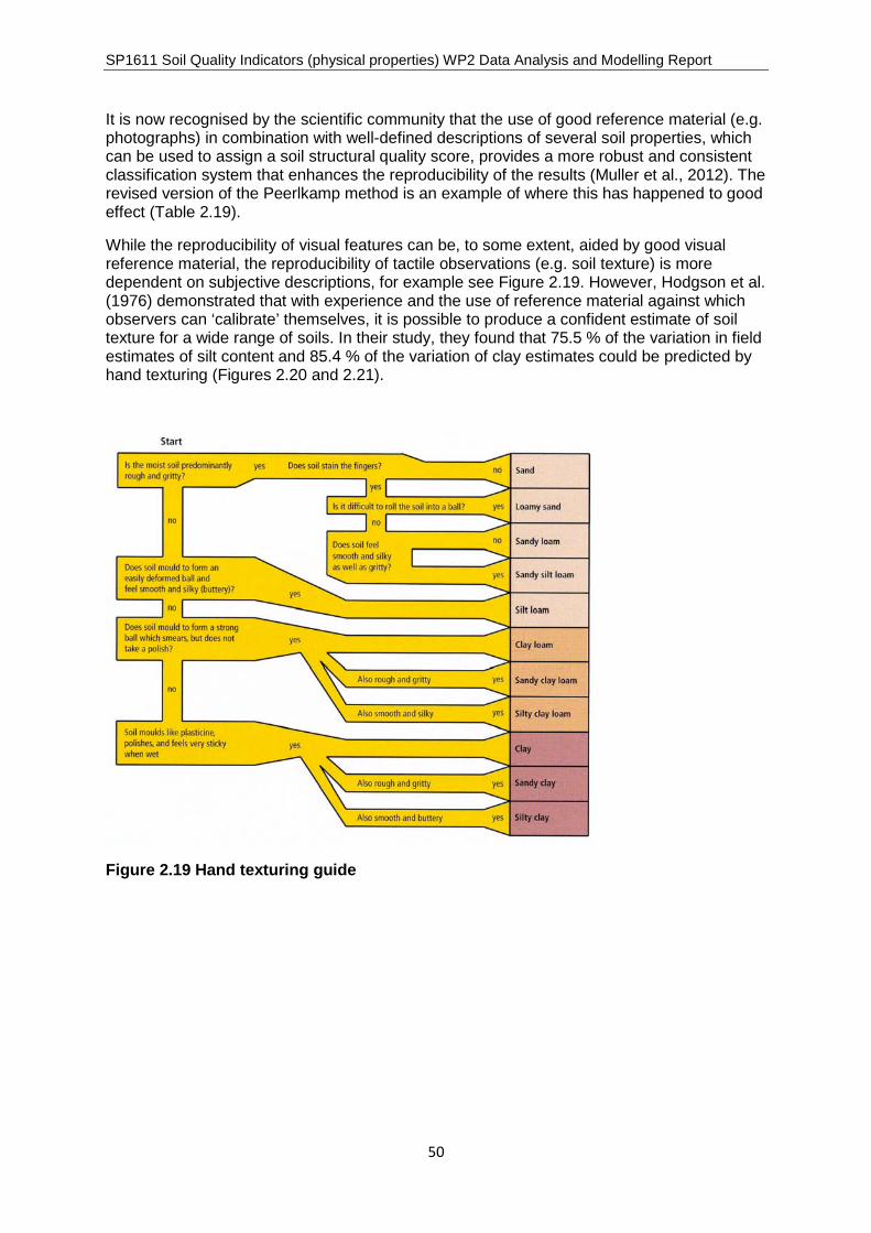
SP1611 Soil Quality Indicators (physical properties) WP2 Data Analysis and Modelling Report
50
It is now recognised by the scientific community that the use of good reference material (e.g.photographs) in combination with well-defined descriptions of several soil properties, whichcan be used to assign a soil structural quality score, provides a more robust and consistentclassification system that enhances the reproducibility of the results (Muller et al., 2012). Therevised version of the Peerlkamp method is an example of where this has happened to goodeffect (Table 2.19).
While the reproducibility of visual features can be, to some extent, aided by good visualreference material, the reproducibility of tactile observations (e.g. soil texture) is moredependent on subjective descriptions, for example see Figure 2.19. However, Hodgson et al.(1976) demonstrated that with experience and the use of reference material against whichobservers can ‘calibrate’ themselves, it is possible to produce a confident estimate of soiltexture for a wide range of soils. In their study, they found that 75.5 % of the variation in fieldestimates of silt content and 85.4 % of the variation of clay estimates could be predicted byhand texturing (Figures 2.20 and 2.21).
Figure 2.19 Hand texturing guide

SP1611 Soil Quality Indicators (physical properties) WP2 Data Analysis and Modelling Report
51
Figure 2.20 Relationship between field estimates (Silte) and laboratory analysis (Silta)of silt (taken from Hodgson et al., 1976)
Figure 2.21 Relationship between field estimates (Claye) and laboratory analyses(Claya) of clay (taken from Hodgson et al., 1976)

SP1611 Soil Quality Indicators (physical properties) WP2 Data Analysis and Modelling Report
52
Could VSE be made numerical through ratings?
One criticism of using VSE as a physical SQI is the lack of quantification by whichmeaningful change (i.e. associated change in soil function) in the SQI is detected. There areboth qualitative and semi-quantitative VSE methods (see Table 2.21).
Table 2.21 Comparison of visual soil evaluation methods and criteria of observations(adapted from Boizard et al., 2005)
Method Reference Key criteria AssessmentWholeprofileassessment
Batey(2000)
Soil texture Soil colour Development, strength and
stability of structure Soil compaction Degree of fissuring Presence of roots
Qualitative. Considers inherentcapability of the soil andlimitations as a result of themanagement of the soil
SOILpak McKenzie(1998)
Size, shape, strength andinternal porosity of primaryclods and aggregates
Factors are weighted andscored between 0.0 (poor) and2.0 (good). Beginners use 3-points (0, 1, 2), experienceduse 5-points (0.0, 0.5, 0.1...),experts use 21-points (0.0, 0.1,0.2...,2.0)
Le profilecultural
Richard etal. (1999)
Transition between the tilledlayers
Internal structural state ofclods or zone
Structural state
Qualitative assessment
Peerlkampscore
Peerlkamp(1959)
Size, shape and porosity ofclods and aggregates
Stability and dispersion onthe surface
Actual or potential rootdevelopment
Scored from 1 (worst ) to 9(best)Modified version (Ball et al.,2007) Scored Sq1 (beststructure) and Sq5 (worststructure) with comparisonphotographs
CWSSC Lawri et al(2000)
Soil texture Stability and resilience of
structure
Non-quantitative
VSA (NZ) Shepherd(2000)
Aggregate size, shape andabundance
Porosity Colour Mottles Erosion Earthworm count
Eight indicators are assessedon a scale of 0.0 (poor) to 2.0(good) (intermediate scoresalso given e.g. 0.5). Judgmentsbased on comparison withphotographs and anundisturbed reference sample.A weighting factor (1, 2 or 3) isapplied to exaggerate moreimportant soil conditionindicators e.g. soil structure
Soil qualityscoring
Ball andDouglas(2003)
Identification of horizontallayers, depth and thickness
Structure Macropores
Separate scores are given foreach criteria on a scale of 1(worst) to 5 (best), using best-fitting descriptions from a

SP1611 Soil Quality Indicators (physical properties) WP2 Data Analysis and Modelling Report
53
Roots and fauna scoring sheet.
VSA(Denmark)
Munkholm(2000)
Soil texture Structure Compaction Anaerobism Root growth Soil fauna Decomposition of organic
matter
No summary into a single score
FALmethod
(seeBoizard etal., 2005)
Size distribution Mean weight diameter Shape, surface, porosity and
cohesion of clods andaggregates
Mean weight score
Score scale 1 (worst) to 14(best). Pictures and key codeshelp classify clod andaggregates into 12 differenttypes.
A guide tobetter soilstructure
Compaction Shape, size, porosity and
consistency of peds
Reference to photographicguide assigning degradationclass: severe, high, moderate,low
Soilstructuraldegradation
Holman etal. (2003)
Surface soil condition Presence of wheeling or
tramlines Extent of poaching Structural changes within or
at the base of topsoil Presence of erosion and
deposition features Vertical wetness gradient
within profile
Qualitative descriptionscategorised into 4 classes(severe, high/extensive,moderate/local, low)
Think Soil EA (2008) Surface erosion features Crop Soil structure Root development
Qualitative
In summary, VSE methods have the potential to be used by researchers, consultants andfarmers. Boizard et al. (2005) identified the potential user groups who may, after appropriatetraining, make use of different VSE methods (see Table 2.22). Most VSE methods can betaught quickly and easily and do not require the skills of a dedicated soil surveyor. Goodreference material helps maintain continuity between observers. However, periodic crosschecking results against other observers is recommended to maintain consistency andeliminate any bad habits.
Semi-qualitative VSE methods provide a value or description against which temporalchanges in score and rankings (the proportion of soils in ‘good’, ‘moderate’ or ‘poor’condition) can be gauged and that can be recorded as an on-going reference. The use ofphotographs as visual records of temporal change is recommended i.e. a visual archive thatcan be related to temporal changes
Semi-quantitative visual evaluation methods could be used to detect large changes instructural quality of the ‘whole topsoil’ over time and for different land uses (e.g. arable andgrassland). A significant cost in monitoring schemes is the time taken for surveyors to travelto monitoring sites and take soil samples. For minimal additional cost (45 minutes to 1 hour

SP1611 Soil Quality Indicators (physical properties) WP2 Data Analysis and Modelling Report
54
per site) visual soil evaluation could be carried out to gain a semi-quantitative assessment ofsoil structural condition that could be monitored over time for individual sites and for thewhole dataset (e.g. does the proportion of sites in good condition change over time?).
Table 2.22 Potential users of each VSE method and the time taken to perform the testin a field (taken from Boizard et al., 2005)
As with other physical SQIs, data uncertainty also comes from timing of assessments.Generally, VSE methods are not easily used when the soil water content is high and the soilis plastic. Neither are they easy to use when the soil water content is very low and cohesionmay be very strong. Spade techniques are also limited in stony soils particularly when thesoil is dry. Concerns over difficulties in breaking up aggregates along natural boundaries byinexperienced operators can be overcome by applying the drop test. However, Guimarães etal. (2011) concluded that both dropping and breaking by hand produced the same score andthe latter was easier and quicker.
It is recognised that some visual characteristics take time to develop and therefore a recentlycompacted site may have fewer visual references than a site where compaction has beenpresent for several seasons. However, repeat observations will help build up a picture overtime that will help define if soil degradation is increasing, decreasing or stable.
As with any other assessment of soil physical properties, VSE methods require trainingbefore a surveyor can use the method in the field with supervision and eventuallyunsupervised.

SP1611 Soil Quality Indicators (physical properties) WP2 Data Analysis and Modelling Report
55
2.12 Integration of physical SQIs
Each candidate physical SQI has been considered independently, but we also consideredthe relationships between the SQIs. There is evidence that combining the measurements ofphysical (and biological and chemical) SQIs improves the relationship between the SQIs, soilprocesses and soil functions. In justifying the use of bulk density / packing density as ameaningful SQI (WP1), we have already seen the empirical evidence suggesting betterprediction of air capacity by combining bulk density and clay content (i.e. Packing density)(Figure 2.21).
Figure 2.21. Improving the relationship between air capacity and measures of bulk /packing density (from Huber et al., 2008)
A similar exercise was done here where data were available (i.e. PD, BD, aggregate stabilityand depth), with the a priori reasoning that a number of the physical SQIs would be inter-dependent and therefore exhibit spatial clustering. However, the resulting cluster analysis ofthe data showed no spatial patterns. This reflects the complexity of relationships betweenthe SQIs and paucity of data. In any case, any relationship between the parameters wouldhave to be expressed in terms of soil processes and functions for it to be meaningful. Eventhe improved relationship between air capacity and packing density (combining clay contentand BD) is only an empirical, rather than explanatory relationship (Huber et al., 2008).
The current project has been focussed on physical properties as soil quality indicators,without explicit reference to biological or chemical SQIs. According to Karlen et al. (2003),soil quality assessment must reflect biological, chemical, and physical properties, processesand their interactions. Taking this more holistic view, Karlen et al. (1997) note theinterdependence among soil quality indicators and that the concept of soil quality should be“an umbrella concept for examining and integrating relationships and functions amongvarious biological, chemical and physical parameters that are measured and important forsustainable agricultural and environmental systems.” They suggest that “field, farm andwatershed-scale evaluations of soil quality require a transition from an experimental modethat contributes to an understanding of soil quality to more interdisciplinary approaches”.Arshad and Martin (2002) identified the interrelationships between a number of key soilquality indicators (physical, biological and chemical; Table 2.23).

SP1611 Soil Quality Indicators (physical properties) WP2 Data Analysis and Modelling Report
56
Table 2.23. Interrelationships of key soil quality indicators (Arshad and Martin, 2002).
Selected indicator Other soil quality indicators affecting the selectedindicator
Aggregation Organic matter, microbial activity (especially fungal),texture
Infiltration Organic matter, aggregation, electrical conductivity(ESP), exchangeable sodium percentage
Bulk density Organic matter, aggregation, topsoil depth, electricalconductivity, biological activity
Microbial biomass and /or respiration
Organic matter, aggregation, bulk density, pH, texture,electrical conductivity
Available nutrients Organic matter, pH, topsoil depth, texture, microbialparameters (mineralisation and immobilisation rates)
These interrelationships have been demonstrated in Fact Sheet 2 (Soil water retentioncharacteristics), where basic soil properties (bulk density, texture and organic C) are used topredict soil water retention characteristics (Dexter’s S, drainable porosity, plant availablewater and relative field capacity) through pedotransfer functions.
Even so, we need to relate these relationships to soil processes and functions. Shukla et al.(2004) carried out step wise regression analysis with corn grain yield as the dependentvariable and measured soil attributes as the independent variables (Table 2.24).
Table 2.24 Linear regression analysis for total dry corn grain yield (Yg, Mg ha-1) asdependent variable and measured soil attributes as independent variables (P<0.009)
Equation R2
One parameter modelYg = 3.753 + 0.007 WSA 0.33
Two parameter model Yg = 3.717 2 0.424 AWC + 0.008 WSA 0.34Yg = 3.353 10.009 WSA – 0.422 MWD 0.34Yg = 14.321 + 0.006 WSA – 1.435 pH 0.34
Three parametermodel
Yg = 23.569 + 0.009 WSA – 0.906 MWD – 2.808 pH 0.37
Yg = 24.061 + 0.007 WSA – 2.809 pH – 2.449 EC 0.36where: AWC – available water (cm); WSA – water stable aggregates (g kg-1); MWD – meanweight diameter (mm); EC – electrical conductivity (dS m-1)
The criticism with this approach is that a) regressions give no explanation of why combiningthese soil properties improves prediction of soil functioning (here, yield); b) the relationshipsand equations would vary for different soil functions (e.g. provisioning v. regulation); c) asreviewed in the WP2 fact sheets above, there are few equivalent data for England andWales linking soil attributes (i.e. physical SQIs) to soil functions; d) this approach takes noaccount / makes no allowance of how a change in one or more attributes over time (which isat the core of a soil monitoring programme) may change the interrelationships between soilattributes; e) the current England and Wales database on physical soil attributes is toolimited and contains too much variability to derive rigorous regression equations.It has been demonstrated that for statistical rigour, the sampling design of each SQI is basedon the detectable / meaningful change in that property (i.e. power analysis). As a result,different SQIs will require different sampling designs, which undermines the concept of

SP1611 Soil Quality Indicators (physical properties) WP2 Data Analysis and Modelling Report
57
having multiple, integrative SQIs, unless the largest sampling size is taken for all. Given thecost implications, we conclude it is impossible to design and implement a rigorous samplingscheme for multiple SQIs.
Another limitation of integrative SQIs is error propagation when using more than one SQI.Error in one or more input variables (e.g. measurement / sampling error) means the resultingintegrative SQI is not robust (Murray Lark, pers.comm.).
2.13 Conclusions to WP2
Data on the physical SQIs selected by the logical sieve process in WP1 are limited in spatialand temporal extent for England and Wales. This has limited the degree of analysis andmodelling that it was possible to test:
the uncertainty in their measurement the spatial and temporal variability in the indicator, as given by observed distributions the expected rate of change in the indicator the impacts on soil processes and functions associated with a change in any given
soil attribute.
Where data are available, power analysis was used to understand the variability of theindicator as given by the observed distributions. This process determines the SQIs ability todetect a particular change at a particular confidence level, given the ‘noise’ or variability inthe data (i.e. a particular power to detect a change of X at a confidence level of Y% wouldrequire N samples).
The paucity in data has limited the specification of a robust sampling design required todetect changes in the SQI that are associated with a meaningful change in any soil processand/or function. In any case, there is little scientific evidence to define what is meant by a‘meaningful change’ in any given SQI and this will vary for different soil types, land coversand soil functions. Attempts were made to stratify detectable changes in packing density andsoil depth by land cover and soil type (Fact Sheet 1 and 5), but no relationships were found.If this had been the case, we would need to relate these changes to associated changes insoil processes and soil functions, but the evidence base is very weak to do this. Schipperand Sparling (2000) identify the challenge: “a standardised methodology may not beappropriate to apply across contrasting soils and land uses. However, it is not practical tooptimise sampling and analytical techniques for each soil and land use for extensivesampling on a national scale”.
Soil hydrological relationships are key to soil functioning, especially in water regulation(availability to plants and avoidance of both flooding and drought; Merrington et al., 2006).Here, the analysis of available data has given promising results regarding the prediction ofvalues of SQIs from easy to measure soil properties (bulk density, texture and organic C),using pedotransfer functions. These measurements also allow estimates of packing densitywhich is also related to soil hydrological properties (e.g. air capacity; Huber et al., 2008).Expanding the evidence base (space and time) should be possible with the developmentand use of rapid, cost-effective techniques using NIR sensors to gain measurements of bulkdensity, texture and packing density.
More evidence is needed as to how aggregate stability affects soil processes and thus soilfunctions. We have found an equivocal relationship with water regulation (runoff generation),which is affected by the method of measurement (low or rapid wetting or mechanicaldisturbance of the aggregates) for example. There are insufficient data on ‘meaningful’change in aggregate stability i.e. how a change in that property affects processes and thus

SP1611 Soil Quality Indicators (physical properties) WP2 Data Analysis and Modelling Report
58
functions. Gathering such data would rely on better, more cost-effective, standardisedmeasurement techniques.
Brazier et al. (2012) used power analyses to estimate the number of monitoring locationsrequired to detect a statistically significant change in soil erosion rate on cultivated land. Onthe basis of this analysis, the project proposed a cost-effective framework to monitor (andmodel) soil erosion in England and Wales, with an emphasis on constructing a statisticallysound approach to locating sampling sites for soil erosion monitoring. However, whatconstitutes a meaningful change in erosion rates still requires data on the impacts of erosionon soil functions in England and Wales.
At present there is insufficient quantified evidence for statistical rigour to be applied indetermining a sampling strategy for Visual Soil Assessments / Evaluations. Some studieshave begun to investigate how VSA might be moved to a quantified scale. Use of remotesensing to detect changes in surface sealing has potential, although the spectral signaturesreceived are not directly measurements of soil quality in terms of physical properties andtheir influence on soil processes and functions. Wood et al. (2004) notes that in general,remote sensing techniques are most useful when considering indicators that relate to soilquantity and have limited utility for those indicators that relate to soil condition (quality). Inany case, as reported in Wood et al (2005), there are few quantified data demonstrating theeffect of soil sealing on soil function, which limits detailed analysis of data.
The scientific robustness of these indicators depends on the availability of spatial andtemporal data, as these reflect the variability of each property (signal to noise ratio), which inturn determines the sampling strategy required to detect significant change. Whether thatchange is meaningful depends on the evidence base relating soil properties to soilprocesses and soil functions. The evidence base is poor: data on meaningful (i.e. whatdegree of change affects soil processes and functions) and detectable (i.e. what sample sizeis needed to detect the meaningful signal from the variability or noise in the signal) arelacking at present to propose a rigorous and reliable soil monitoring programme.

SP1611 Soil Quality Indicators (physical properties) WP2 Data Analysis and Modelling Report
59
ReferencesAhmadi A, Neyshabouri M-R, Rouhipour H and Asadi H 2011. Fractal dimension of soil
aggregates as an index of soil erodibility. Journal Of Hydrology Volume: 400 Issue: 3-4Pages: 305-311
Amézketa, E. 2008. Soil aggregate stability: a review. Journal of Sustainable Agriculture, 14:2-3; 83-151.
Arshad, M.A. and Martin, S. 2002. Identifying critical limits for soil quality indicators in agro-ecosystems. Agriculture, Ecosystems and Environment 88 (2002) 153–160.
Arshad, M.A., Lowery, B., Grossman, B., 1996. Physical tests for monitoring soil quality. In:Doran, W., Jones, J. (Eds.), Methods for Assessing Soil Quality, Madison, WI, 1996. SoilSci. Soc. Am. 49, 123–141 (special publication).
Arvidsson, J. (1998). Influence of soil texture and organic matter content on bulk density, aircontent, compression index and crop yield in field and laboratory compressionexperiments. Soil and Tillage Research, 49: 159-170.
Australian Natural Resources Atlas accessed on line athttp://www.anra.gov.au/topics/soils/pubs/national/agriculture_asris_depth.html, August2012
Avery BW and Bascomeb CL (1982) Soil Survey Laboratory Methods. Soil Survey TechnicalMonograph No 6, pp83. Harpenden, UK
Baatz, M. and Schape, A. 2000. Multi-resolutional Segmentation - an optimization approachfor high quality multi-scale image segmentation. AGIT-Symposium Salzburg 2000, pp. 12-23.
Baatz, M., Heynen, M., Hofmann, P., Lingenfelder, I., Mimler, M., Schape, A., Weber, M. andWillhauck, G. 2000. eCognition User Guide. Definiens AG. Munich.
Ball BC and Douglas JT (2003). A simple procedure for assessing soil structural, rooting andsurface conditions. Soil Use and Management 19, 50-56.
Ball BC, Batey T, Munkholm LJ (2007). Field assessment of soil structural quality—adevelopment of the Peerlkamp test. Soil Use and Management 23, 329–337.
Batey T. 2000. 15. Soil profile description and evaluation. in Smith KA & Mullins CE Eds. Soiland Environmental Analysis: physical methods 2nd Edition. New York : Marcel Dekker,Inc.
Beven, K., Young, P., Romanowicz, R., O’Connell, E., Ewen, J., O’Donnell, G., Holman, I.,Posthumus, H., Morris, J., Hollis, J., Rose, S., Lamb, R., Archer, D., 2008. Analysis ofhistorical data sets to look for impacts of land use and management change on floodgeneration. Defra R&D Final Report FD2120.
Boardman J and Poesen J (2006) Soil Erosion in Europe. John Wiley and Sons, UK. 855 pp.
Boizard H, Batey T, McKenzie D, Richard G, Roger-Estrade J, Ball B, Bradley I, Cattle S,Hasinger G, Munkholm L, Murphy B, Nievergelt J, Peigné J and Shepherd G (2005) Fieldmeeting “Visual Soil Structure Assessment” Held at the INRA Research Station, Estrées-Mons, France 25-27 May 2005.
Brazier R, Anderson K, Bellamy P, Ellis M, Evans M, Quine T, Quinton JN, Rawlins B,Rickson, RJ. 2012. Developing a cost-effective framework for monitoring soil erosion inEngland and Wales. Final Report to Defra: Project SP1303: 2012.
Bryan, R.B., 1968. The development, use and efficiency of indices of soil erodibility.Geoderma, 2(1): 5-26.
Bui EN, Hancock GJ, Chappell A and Gregory LJ (2010) Evaluation of totlerable erosionrates and time to critical tipsoil loss in Australia. CSIRO Land and Water, Canberra
Caprioli, M. and Tarantino, E. 2003. Urban features recognition from VHR satellite data withan object-oriented approach. Proceedings of Commission IV Joint Workshop (CD-ROM),
SP1611 Soil Quality Indicators (physical properties) WP2 Data Analysis and Modelling Report
60
Challenges in Geospatial Analysis, Integration and Visualization II, September 8–9, 2003,Stuttgart, Germany (2003).
Chambers, B. J., Davies, D. B., and Holmes, S. 1992 Monitoring of water erosion on arable
farms in England and Wales, 1989-90. Soil Use and Management 8, 163-170.
Cockroft, B., Olsson, K.A., 1997. Case study of soil quality in south-eastern Australia:management of structure for roots in duplex soils. In: Gregorich, E.G., Carter, M.R.(Eds.), Soil Quality for Crop Production and Ecosystem Health. Developments in SoilScience, vol. 25. Elsevier, New York, NY, pp. 339 – 350.
Cooper S (2007) The role of conservation soil management on soil and water protection atdifferent spatial scales. PhD Thesis, Cranfield University.
Da Silva, A.P., Kay, B.D. and Nadler, A. (2001). Factors contributing to temporal stability inspatial patterns of water content in the tillage zone. Soil and Tillage Research, 58: 207-218.
Dam, R.F., Mehdi, B.B., Burgess, M.S.E., Madramatoo. C.A., Mehuys, G.R. and Callum, I.R.(2005). Soil bulk density and crop yield under eleven consecutive years of corn withdifferent tillage and residue practices in a sandy loam soil in Central Canada. Soil andTillage Research, 84: 41-53.
Davidson, D.A. and Wilson, C.A. 2006. An assessment of potential soil indicators for thepreservation of Cultural Heritage. . Final report. Defra project SP0554
De Coursey, D.G. and Meyer, L.D. (1977) Philosophy of erosion simulation for land usemanagement. In: Foster, G.R. (ed.) Soil Erosion: Prediction and Control. Proceedings of anational conference on soil erosion, Purdue University, West Lafayette, Indiana. SoilConservation Society of America, Ankeny, IA, pp. 193–200.
Department for Communities and Local Government have detailed the National PlanningPolicy Framework (March 2012),http://www.communities.gov.uk/documents/planningandbuilding/pdf/2116950.pdf
Dexter, A.R. & Bird, N.R.A. 2001. Methods for predicting the optimum and the range of soilwater contents for tillage based on the water retention curve. Soil and Tillage Research ,57, 203-212.
Dexter, A.R. & Czyz, E.A. 2007. Applications of s-theory in the study of soil physicaldegradation and its consequences. Land Degradation and Development , 18, 369-381.
Dexter, A.R. 2004a. Soil physical quality: Part I. Theory, effects of soil texture, density, andorganic matter, and effects on root growth. Geoderma , 120, 201-214.
Dexter, A.R. 2004b. Soil physical quality; Part II. Friability, tillage, tilth and hard-setting.Geoderma, 120, 215-225.
Dexter, A.R. 2004c. Soil physical quality; Part III: Unsaturated hydraulic conductivity andgeneral conclusions about S theory. Geoderma, 120, 227-239.
Dexter, A.R., Richard, G. 2009. Tillage of soils in relation to their bi-modal pore sizedistributions, Soil Till. Res., 103, 113-118.
EEA soil sealing, 2012. http://www.eea.europa.eu/data-and-maps/data/eea-fast-track-service-precursor-on-land-monitoring-degree-of-soil-sealing-100m-1
Environment Agency (2008) Think Soils. Published by the Environment Agency, Bristol.
EU DG Environment, 2012. Science for Environmental Policy, DG Environment News AlertService. In-depth report: Soil Sealing, March 2012.
Evans R. 2002. An alternative way to assess water erosion of cultivated land - field-basedmeasurements: and analysis of some results. Applied Geography 2002; 22(2): 187-207.
Evans R., & Cook S., (1986) Soil Erosion in Britain. SEESOIL (3) 28-58
Gaţe, O.P., Czyż, E.A., Dexter, A.R. 2006. Soil physical quality, S, as a basis for relationships between some key physical properties of arable soils. Proceedings of

SP1611 Soil Quality Indicators (physical properties) WP2 Data Analysis and Modelling Report
61
International Soil Tillage Research Organisation, 17th Triennial Conference 28 August–3September, Kiel, Germany pp 258-264
GeoInformation Group 2012, National Land Use Maphttp://www.geoinformationgroup.co.uk/products/national-lu
Gomez AA, Swete Kelly DE, Syers JK and Coughtan KJ (1996). Measuring sustainability ofagricultural systems at the farm level. In: Doran W and Jones J (Eds) Methods forAssessing Soil Quality, Madison, WI. Soil Sci Soc. Am. 49: 401-410
Graves A, Morris J, Deeks LK, Rickson J, Kibblewhite MG, Harris JA and Farewell TS (2011)The Total Costs of Soils Degradation in England and Wales. Final project (SP1606)report to Defra.
Gregory AS Webster CP Watts CW Whalley WR (2010). The effect of different grass speciesand their different hybrids on soil hydraulic properties. Soil Science Society AmericaJournal 74: 753-761
Gregory AS, Watts CW Whalley WR Kuan HL Griffiths BS Hallett PJ Whitmore AP (2009).The effect of long-term soil management on the physical and biological resilience ofarable and grassland soils in England. Geoderma. 153: 172-185.
Gregory, A.S., Watts, C.W., Griffiths, B.S., Hallett, P.D., Hsueh, L.K. and Whitmore, A.P.(2009). The effect of long-term soil management on the physical and biological resilienceof a range of arable and grassland soils in England. Geoderma, 153, 172-185.
Guimarães RML, Ball BC and Tormena CA (2011) Improvements in the visual evaluation ofsoil structure. Soil Use and Management, 27: 395-403.
Hakansson, I. (1990). A method for characterizing the state of compactness of the ploughlayer. Soil and Tillage Research, 16: 105-120.
Hall, D.G.M., Reeve, M.J., Thomasson, A.J. and Wright, V.F. (1977). Water Retention,Porosity and Density of Field Soils. A.R.C. Soil Survey Technical Monograph 9.Harpenden.
Hill RB, Sparling G, Frampton C and Cuff J (2003) National Soil Quality Review andProgramme Design.
Hodgson JM, Hollis JM, Jones RJA and Palmer RC (1976) A comparison of field estimatesand laboratory analyses of the silt and clay contents of some west Midland soils. Journalof Soil Science, 27: 411-419.
Hodgson, J.M. (1976) Soil Survey Field Handbook – Describing and Sampling Soil Profiles.Soil Survey Technical Monograph No.5. Adlard & Son Ltd.1976. 99pp.
Holman IP, Hollis JM, Bramley ME and Thompson TRE (2003) The contribution of soilstructural degradation to catchment flooding: a preliminary investigation of the 2000floods in England and Wales. Hydrology and Earth System Sciences, 7: 755-766.
Houšková B (2005) Visual Soil Assessment. 3rd European Summer School on Soil Survey,co-organized by TAIEX, JRC and SZIU.
Huber, S., G. Prokop, D. Arrouays, G. Banko, A. Bispo, R.J.A. Jones,M.G. Kibblewhite, W.Lexer, A. Möller, R.J. Rickson, T. Shishkov, M. Stephens, G. Toth, J.J.H. Van den Akker,G. Varallyay, F.G.A. Verheijen, A.R. Jones (eds). 2008. Indicators & Criteria report.Environmental Assessment of Soil for Monitoring (ENVASSO) Volume I: EUR 23490EN/1 – 2008.
Huber, S., Prokop, G., Arrouays, D., Banko, G., Bispo, A., Jones, R.J.A., Kibblewhite, M.G.,Lexer, W., Möller, A., Rickson, R.J., Shishkov, T., Stephens, M., Toth, G. Van den Akker,J.J.H., Varallyay, G., Verheijen, F.G.A. and Jones, A.R. (eds) (2008). EnvironmentalAssessment of Soil for Monitoring: Volume I Indicators & Criteria. EUR 23490 EN/1,Office for the Official Publications of the European Communities, Luxembourg, 339pp.
Jones, C.A. 1983. Effect of soil texture on critical bulk densities for root growth. Soil Sci. Soc.Am. J. 47, 1208–1211.

SP1611 Soil Quality Indicators (physical properties) WP2 Data Analysis and Modelling Report
62
Kampouraki, M., Wood, G.A., Brewer, T.R. 2008. Opportunities and limitations of objectbased image analysis for detecting urban impervious and vegetated surfaces using true-colour aerial photography. In: Object-based Image Analysis: Spatial Concepts forKnowledge-Driven Remote Sensing Applications. Springer-Verlag. pp. 555-570.
Karlen, D.L., Ditzler, C.A. and Andrews, S.S. 2003. Soil quality: why and how? Geoderma,Volume 114, Issues 3–4, June 2003, Pages 145-156.Kibblewhite, M. 2007. Towards a European soil directive – the rational and somereflections. Environmental Law and Management, 19(5), pp 227-231.
Karlen, D.L., Ditzler, C.A. and Andrews, S.S. 2003. Soil quality: why and how? Geoderma,Volume 114, Issues 3–4, June 2003, Pages 145-156.
Kibblewhite, M., Rubio, J.-L., Kosmas, C., Jones, R., Arrouays, D., Huber, S., Verheijen, F.,2007. Environmental assessment of soil for monitoring desertification in Europe. EighthSession of the Conference of the Parties (COP 8) to the United Nations Convention toCombat Desertification (UNCCD). Cranfield University, UK, Madrid, Spain, p. 62. 3–14September 2007, ISBN 1-8713115-97-2.
Kosmas, C., Gerontidis, St., and Marathainou, M. 2000. The effect of land use change onsoil and vegetation over various lithological formations on Lesvos (Greece). Catena,40:51-68.
Kosmas, C., Gerontidis, St., Marathianou, M., Detsis, V., and Zafiriou, Th. 2001. The effectof tillage erosion on soil properties and cereal biomass production. Soil & TillageResearch J. 58:31-44
Kuang B, Mahmood HS, Quraishi Z, Hoogmoed WB, Mouazen A M and van Henten EJ(2012) Sensing soil properties in the laboratory, in situ, and on-line: a review. In DonaldSparks, editors: Advances in Agronomy, 114: 155-244
Kurz, I., O’Reilly, C.D. and Tunney, H. (2006). Impact of cattle on soil physical propertiesand nutrient concentrations in overland flow from pastures in Ireland. Agriculture,Ecosystems and Environment, 113: 378-390.
Lal R (1993) Tillage effects on soil degradation, soil resilience, soil quality, and sustainability.Soil & Tillage Research, 27: 1-8
Lal R, Ahmadi M and Bajracharya RM (2000) Erosional impacts on soil properties and cornyield on Alfisols in central Ohio. Land Degradation & development, 11: 575-585.
Lal, R., 1998. Soil erosion impact on agronomic productivity and environmental quality.Critical reviews in plant sciences, 17 (4), 319-464.
Lark, R. M. (2009), "Estimating the regional mean status and change of soil properties: twodistinct objectives for soil survey", European Journal of Soil Science, vol. 60, no. 5, pp.748-756.
Lark, M., Rawlins, B.G. Robinson, D.A. Robinson, I. Tye, A.. 2012. Studies to inform policydevelopment with regard to soil degradation (Subproject B, Determination of soil bulkdensity). Final report to Defra, SP1305.
Lawrie, J, Murphy, B, Packer, IJ and Harte, AJ (2000). Soils and sustainable farmingsystems. In PEV Charman and BW Murphy (eds). Soils – Their Properties andManagement. (Oxford University Press, Melbourne)
Le Bissonnais, Y. (1996). Aggregate stability and assessment of soil crustability anderodability: I. Theory and methodology. European Journal of Soil Science, 47, 425-437.
Leprêtre, A., Martin, S., 1994. Sampling strategy for soil quality. Anal. Mag. 33, 40–43.
Logsdon, S.D. and Karlen, D.L. 2004. Bulk density as a soil quality indicator duringconversion to no-tillage. Soil & Tillage Research 78 (2004) 143–149
Mackay, A.D., Simcock, R., Sparling, G.P., Vogler, I. and Francis, G. (2006). Macroporosity.Internal SLURI report. Agresearch, Hamilton.

SP1611 Soil Quality Indicators (physical properties) WP2 Data Analysis and Modelling Report
63
Matthews GP Watts CW Powlson DS Price JC & Whalley WR (2008) Wetting of agriculturalsoils measured by a simplified capillary rise technique. European Journal of Soil Science.59: 817-823.
Matula S, Mojrová M and Špongrová (2007) Estimation of the soil water retention curve(SWRC) using pedotransfer functions (PTFs). Soil & Water Research, 2: 113-122.
Mayr T and Jarvis NJ (1999) Pedotransfer functions to estimate soil water retentionparameters for a modified Brooks-Corey type model. Geoderma 91: 1-9.
McHugh, M., (2007) Short-term changes in upland soil erosion in England and Wales: 1999to 2002. Geomorphology 86 (1-2), 204-213
McHugh, M., Harrod, T., and Morgan, R., (2002) The extent of soil erosion in uplandEngland and Wales. Earth Surf. Process. Landforms 27 (1), 99-107.
McIntyre N; Marshall M (2010). Identification of rural land management signals in runoffresponse. Hydrological Processes 24(24): 3521-3534
McKenzie DC (Ed.) (1998) ‘SOILpak for cotton growers, third edition..’ (NSW Agriculture:Orange)
Meinel, G. and Hernig, A. 2005. Survey of soil sealing on the basis of the ATKIS basic DLM– feasibilities and limits. 10th International Conference of Information & CommunicationsTechnologies (ICT) in Urban Planning and Spatial Development and Impacts of ICT onPhysical Space, 22-25 Feb. 2005.
Merrington G, Fishwick S, Barraclough D, Morris J, Preedy N, Boucard T, Reeve M, Smith Pand Fang C (2006) The development and use of soil quality indicators for assessing therole of soil in environmental interactions. Environment Agency Science ReportSC030265, Bristol, UK
Moebius, B.N., van Es, H.M., Schindlebeck, R.R., Idowu, J.O., Clune, D.J. and Thies, J.E.2007. Evaluation of laboratory measured soil properties as indicators of soil physicalquality. Soil Science, 172, No 11. P 895-912.
Morgan RPC, 2005. Soil Erosion and Conservation. Blackwell, Oxford, 304 pp.
Mouazen, A.M and Ramon, H. (2006). Development of on-line measurement system of bulkdensity based on on-line measured draught, depth and soil moisture content. Soil andTillage Research, 86(2): 218-229.
Mueller L, Kay BD, Deen B, Hu C, Zhang Y, Wolff M, Eulenstein F, Schindel U (2009b)Visual assessment of soil structure: Part II. Implications of tillage, rotation and traffic onsites in Canada, China and Germany. Soil & Tillage Research, 103: 188-196.
Mueller L, Kay BD, Hu C, Li Y, Schindle U, Behrendt A, Shepherd TG and Ball BC (2009a)Visual assessment of soil structure: Evaluation of methodologies on sites in Canada,China and Germany. Part I: Comparing visual methods and linking them with soil physicaldata and grain yield of cereals. Soil & Tillage Research, 103: 178-187.
Mueller L, Shepherd G, Schindler U, Ball BC, Munkholm LJ, Hennings V, Smolentseva E,Rukhovic O, Lukin S and Hu C (2012) Evaluation of soil structure in the framework of anoverall soil quality rating. Soil & Tillage Research, doi:10.1016/j.still.2012.03.002
Munkholm, L.J. (2000). The spade analysis - a modification of the qualitative spadediagnosis for scientific use. DIAS-report No. 28 Plant Production, Danish Institute ofAgricultural Sciences.
Newell Price JP, Chambers BJ Whittingham MJ. (2012a) Characterisation of Soil StructuralDegradation Under Grassland and Development of Measures to Ameliorate its Impact onBiodiversity and Other Soil Functions BD5001: Final report to Defra.
Newell Price JP, Whittingham MJ, Chambers BJ and Peel S (2012b) Visual soil evaluation inrelation to measured soil physical properties in a survey of grassland soil compaction inEngland and Wales, Soil & Tillage Research, doi:10.1016/j.still.2012.003
Nielsen DR, Biggar JW and Erh KT (1973) Spatial variability of field-measured soil-waterproperties. Hilgardia, 42: 215-259

SP1611 Soil Quality Indicators (physical properties) WP2 Data Analysis and Modelling Report
64
O’Connell, P.E., Beven, K.J., Carney, J.N., Clements, R.O., Ewen, J., Fowler, H., Harris,G.L., Hollis, J., O’Donnell, G.M., Packman, J.C., Parkin, A., Quinn, P.F., Rose, S.C.,Shepherd, M., Tellier, S., 2004. Review of impacts of rural land management on floodgeneration. Impact Study Report. Defra R&D Technical Report FD2114/TR.
O’Connell, P.E., Ewen, J., O’Donnell, G., Quinn, P., 2007. Is there a link betweenagricultural land-use management and flooding?, Hydrol. Earth Syst. Sci., 11, 96-107.
Peerlkamp PK.(1959). A visual method of soil structure evaluation.Meded. V.d.Landbouwhogeschool en Opzoekingsstations van deStaat te Gent, XXIV, 216–221.
Pimental D, Harvey C, Resosudarmo P, Sinclair K, Kurz D, McNair M, Crist S, Sphpritz L,Fitton L, Saffouri R and Blair R (1995) Environmental and economic costs of soil erosionand conservation benefits. Science, 267, 117-1123
Quine TA, Walling DE. Rates of soil erosion on arable fields in Britain: quantitative data fromCaesium-137 measurements. Soil Use and Management 1991;7:169-176.
Quinton J.N., Catt, J.A. Wood, G.A. and Steer, J. 2006. Soil carbon losses by water erosion:Experimentation and modeling at field and national scales in the UK. Agriculture,Ecosystems and Environment 112 (2006) 87–102
Rawlins, B.G., Wragg, J. and Lark, R.M. undated. Application of a novel method for soilaggregate stability measurement by laser granulometry with sonication.
Reynolds, W.D., Bowman, B.T., Drury, C.F., Tan, C.S., Lu, X. 2002. Indicators of good soilphysical quality: density and storage parameters. Geoderma , 110, 131-146.
Reynolds, W.D., Drury, C.F., Tan, C.S., Fox, C.A. & Yang, X.M. 2009. Use of indicators andpore volume-function characteristics to quantify soil physical quality. Geoderma , 152,252-263.
Richard G, Boizard H, Roger-Estrade J, Boiffin J and Gu‚rif J (1999) Field study of soilcompaction due to traffic in northern France: pore space and morphological analysis ofcompacted zones. Soil and Tillage Research 51, 151-160
Richards, J.A., and Jia, X. 2005. Remote sensing digital image analysis. Springer.
Rickson, R.J. 2006. Management of sediment production and prevention in river catchments:A matter of scale? In Collins, A.J. and Owens, P. (eds.) Soil erosion and sedimentredistribution in river catchments: measurement, modelling and management in the 21stcentury. CAB International. pp 228-238.
Robinson, D.A., D. Cooper, B.A. Emmett, C.D. Evans, A. Keith, I. Lebron, S. Lofts, L.Norton, B. Reynolds, E. Tipping, B.G. Rawlins, A.M. Tye, C.W. Watts, W.R. Whalley,H.I.J Black, G.P. Warren, S. Robinson, K. Michaelides, N.J. Hockley. 2010. Defra soilprotection research in the context of the soil natural capital / ecosystem servicesframework. In, Project SP1607: Synthesis of Soil Protection work 1990-2008. Centre forEcology and Hydrology, UK.
Saygin, S.D., Cornelis, W.M., Erpul, G. and Gabriels, D. 2012. Comparison of differentaggregate stability approaches for loamy sand soils. Applied Soil Ecology 54 (2012) 1– 6
Shepherd TG (2000) Visual soil assessment. Volume 1. Field guide for cropping andpastoral grazing on flat to rolling country. horizons.mw/Landcare Research, PalmerstonNorth. 84 p.
Shepherd TG (2008) Visual Soil Assessment. Volume 1. Field guide for pastoral grazing andcropping on flat to rolling country. 2 nd edition. Palmerston North, New Zealand, HorizonsRegional Council. 106 pp.
Shepherd TG and Park SC (2003) Visual Soil Assessment: A Management Tool For DairyFarmers. In: Brookes IM ed. Proceedings of the 1st Dairy Conference. ContinuingMassey University Dairy Farming Annual (Volume 55) Dexcel’s Ruakura Dairy farmers’’Conference, April 7-9, 2003, Rotorua. Pp 111-123.
SP1611 Soil Quality Indicators (physical properties) WP2 Data Analysis and Modelling Report
65
Shukla, M.K., Lal, R. and Ebinger, M. 2004. Soil Quality Indicators for the North Appalachianexperimental watersheds in Coshocton Ohio. Soil Science, Volume 169, Issue 3, 195-205.
Smith, G., Beare, M., Boyd, M., Downs, T., Gregory, M., Morton, D., Brown, N. andThomson, A. 2007. UK Land Cover Map Production through Generalisation of OSMasterMap. The Cartographic Journal, 44(3), pp 276-283.
Smith, R and Quinton, J.N. (2000) Dynamics and scale in simulating erosion by water. In:Schmidt, J. (ed.) Soil Erosion: Application of Physically Based Models. Springer, Berlin,pp. 282–294.
Stallings, J.H. 1964. Phosphorus and water pollution. Journal of Soil Water andConservation 22: 228-231.
Stavi I, Ungar ED, Lavee H and Sarah P (2011) Soil aggregate fraction 1- 5 mm: Anindicator for soil quality in rangelands. Journal of Arid Environments, 75: 1050-1055
Stocking M and Pain A (1983) Soil life and the minimum soil depth for productive yields:developing a new concept. Discussion Paper No. 150, School of Development Studies,University of East Anglia, Norwich vide Bojö, 1991a.
Taylor, M.D., Kim, N.D., Hill, R.B. and Chapman, R. (2010). A review of soil quality indicatorsand five key issues after 12 yr soil quality monitoring in the Waikato region. Soil Use andManagement, 26: 212-224.
Thompson TRE and Peccol EC 1995. Sustaining Land Resources: The Role of SoilInformation in Planning the Sustainable Use of Land Resources. Soil Survey and LandResearch Centre.
Tucker, C.J., 1979, Red and photographic infrared linear combinations for monitoringvegetation. Remote Sensing of Environment, 8, pp. 127–170.
van Genuchten, M.T. 1980. A closed form equation for predicting the hydraulic conductivityof unsaturated soils. Soil Science Society of America Journal , 44, 892-8.
Van Noordwijk, M., van Roode, M., McCaillie, E.L. and Lusiana, B. (1998) Erosion andsedimentation as multi-scale, fractal processes: implications for models, experiment andthe real world. In: Penning de Vries, F.W.T., Agus, F. and Kerr, J. (eds) Soil Erosion atMultiple Scales: Principles and Methods for Assessing Causes and Impact. CABInternational, Wallingford, pp. 223–253.
Van Rompaey, A.J.J., Vieillefont, V., Jones, R.J.A., Montanarella, L., Verstraeten, G,Bazzoffi P., Dostal, T, Krasa, J, de Vente, J., Poesen, J.. Validation of soil erosionestimates at European scale. European Soil Bureau Research Report No.13, EUR 20827EN, (2003), 26pp. Office for Official Publications of the European Communities,Luxembourg.
Verheijen FGA, Jones RJA, Rickson RJ and Smith CJ (2009) Tolerable versus actual soilerosion rates in Europe. Earth-Science Reviews, 94, 23-38
Verheijen, F.G.A., Jones, R.J.A., Rickson, R.J., and Smith, C.J. 2009 Tolerable versusactual soil erosion rates in Europe. Earth-Science Reviews, 94: 23-38
Walling, D.E., Quine, T.A., 1991. Use of 137Cs measurements to investigate soil erosion onarable fields in the UK: potential applications and limitations. Journal of Soil Science, 42(1), 147–165.
Walling, D., Zhang, Z., and Parker A. (2005) Documenting soil erosion rates on agriculturalland in England and Wales. Research report to DEFRA, SP0411, Exeter University.
Walling, D., Zhang, Z., and Parker A. (2008) Documenting soil erosion rates on agriculturalland in England and Wales – Part 2. Research report to DEFRA, SP0413, ExeterUniversity.
Watts CW Dexter AR Arvidsson J Czyz EA. (2000c). The effects of simulated tillage and soilfactors on soil respiration. Proceedings 15th ISTRO-2000, Fort Worth , TX . July 1-7,2000

SP1611 Soil Quality Indicators (physical properties) WP2 Data Analysis and Modelling Report
66
Watts CW Dexter AR. 1997. The influence of organic matter in reducing the destabilisationof soil by simulated tillage. Soil and Tillage Research, 42, 253-275.
Watts CW Dexter AR. 1998. Soil friability: theory, measurement and the effects ofmanagement and organic carbon content. European Journal of Soil Science: 49, 73-84.
Watts CW Whalley WR Longstaff, DJ White RP Brookes PC Whitmore AP 2001.Aggregation of soil with different cropping histories following the addition of differentorganic materials. Soil Use and Management 17, 1–6
Wood, G.A., Loveland, P.J. and Kibblewhite, M.G. 2004. The use of remote sensing todeliver soil monitoring. Final report to Defra, SP0541.
Wood, G.A., Kibblewhite, M.G., Hannam, J.A., Harris, J.A. and Leeds-Harrison, P.B. 2005.Soil-Based Services In The Built Environment. A report prepared for the Department ofEnvironment, Food and Rural Affairs.

SP1611 Soil Quality Indicators (physical properties) WP2 Data Analysis and Modelling Report
67
APPENDIX 1.Notes of a meeting held on 18/04/12 to discuss progress on WP2 Data analysis and modellingBackgroundTo summarize, a set of possible physical SQIs
2were evaluated through the logical sieve. A number of
indicators were identified in WP1 and Defra are generally happy with these. These are made up of thetop 25% overall scoring indicators and all SQIs that passed the logical sieving process. So theindicators under consideration are now:
Physical SQI’s Champion1. Bulk density (FDR and VIS-NIR spectroscopy method) AM2. Depth of soil JR; LD3. Infiltration / drainage capacity PNP; CK4. Moisture storage capacity / Soil water retention characteristics PNP; CK; TW5. Number of erosion features JR6. Packing density BJ; PNP; LD7. Profile description LD; PNP8. Rate of erosion JR9. Sealing TW10. Shear strength (Going Stick method) IJ11. Soil structure CK LD12. Soil texture (wet sieving and sedimentation methods) CK LD13. Surface water turbidity IH14. Total porosity CK RC15. Bulk density (Kopecki ring) PNP16. Erodibility / aggregate stability JR17. Biological status IH18. Number of eutrophication incidents IH
AM Abdul Mouazen BJ Bob Jones CK Cedric KechavarziIH Ian Holman IJ Iain James, JR Jane RicksonLD Lynda Deeks PNP Paul Newell Price RC Ron CorstanjeTW Toby Waine
Feedback from Defra / Declan Barraclough of key issues to be addressed in Work Package 2 Robustness (reliability and accuracy) of the indicator, both statistical and practicability Relevance – can it realistically be interpreted in terms of a key soil function? Synergy – is there scope for combining with another indicator to greater effect? Cost
Moving forward, there are two objectives related to WP2: Objective 2.1: Evaluation of new scientific evidence, reports, data, SQI selection criteria, sampling
techniques and monitoring methodologies aimed at identifying salient physical SQIs (by the endof Project Month 8)
Objective 2.2: Identification of suitable physical SQIs from the findings of Objectives 1.1 and 2.1above, based on agreed selection criteria, sound science, statistical robustness and feasible datacollection methods (by the end of Project Month 9)
2Key indicator criteria are (see EPA's Report on the Environment):
An indicator is a numeric value derived from actual measurements of a pressure, state or ambient condition over a specified
geographic domain, whose trends over time represent or draw attention to underlying trends in the condition (or "health") of the
environment.
the indicator is useful;
the indicator is objective;
the indicator is transparent and reproducible;
the underlying data is characterized by sound collection methodologies, data management systems to protect its integrity, andquality assurance procedures;
data are available to describe changes or trends; and
the data are comparable across time and space, and representative of the target population.

SP1611 Soil Quality Indicators (physical properties) WP2 Data Analysis and Modelling Report
68
Regarding the scientific evidence; there are, for all intents and purposes, two soil functions that aredirectly affected by changes in soil physical properties: i) the production function and ii) the regulationfunction. These indicators would be measures that indicate a degree of degradation in these soilfunctions. What we are trying to get a feel for is the effect-response curve of these indicators todegradation in these soil functions and, from this, the cost effectiveness of the indicator. In summary,what we need to know for each indicator is
1. What is it indicative of; i.e. what function is being degraded?2. What it is responsive to? How responsive is it? sensitivity, responsiveness3. What factors may mitigate or accentuate the response? e.g. soil type, land use4. Is this indicator a first order indicator (i.e. a direct measure of the change in soil quality) or
a second, third, etc order indicator (i.e. an indirect measure of the change; e.g. VNIRS,remote sensing)?
Regarding reports, data. In order to meet objective 2.2, we will need to analyse suitable candidates,and for this we will need data, so
5. Please identify existing or suspected data-holdings for each indicator.
Regarding SQI selection criteria, sampling techniques and monitoring methodologies.We will need toreduce this list of indicators as I don’t think it feasible to analyse all 18 SQI’s. The logical sieve hashelped us rank and organize much of the information currently, but a national monitoring schemecannot include 18 physical SQIs due to the resource implications nor will we be able within this projectto investigate 18 SQIs
6. How is it measured?7. What sampling support does it need?8. What is the sampling intensity required?
Notes of the meeting 18/04/2012Present: Abdul Mouazen, Paul Newell Price (ADAS), Lynda Deeks, Pat Bellamy, Iain James, CedricKechavarzi, Jane Rickson, Ron Corstanje.Apologies: Ian Holman, Toby Waine.Aims: Revisit the outcome of WP1, especially the Logical Sieve exercise to ensure the results were
sensible and that no indicators were disqualified unduly. Move from the ‘narrative’ of WP1 to a more ‘numerical’ approach in WP2 i.e. given the remaining
SQIs, are data available to test the robustness of the candidate SQIs through statistical/modellinganalysis?
Rationalise the remaining SQIs in terms of duplications (e.g. total porosity ≈ 1- BD/particle density); overlaps /double counting (e.g. no. of erosion features and rate of erosion); and linkages(e.g. BD and depth – the Logical Sieve consider all candidate SQIs as independent of each other– are composites useful?)
Consider scale issues e.g. scaling up / aggregating SQI performance at the field (or equivalent onnon-ag land) to larger landscape units.
Initially a number of general points were discussed regarding the concept of soil quality indicators.What makes a ‘good’ soil indicator and why?a) It needs to be sensitive and responsive to the loss or degradation of soil functions. Points were
raised regarding the soil functionsi. It was generally agreed that the most common functions we’ll consider are the production
and regulation functions.ii. Not every indicator will be appropriate for any given function e.g. loss in depth of soil
impacts regulation function immediately, but less immediate on production function if soilsare deep and rooting depth is not limiting.
iii. The basic spatial unit for assessing soil functions is the field scale. This is because it isexpected that this is the most appropriate scale to link the relationship between soilproperties and the production /regulation function of soils. It is the scale at whichmanagement options would be practiced. At the larger scale (e.g. catchment), these linksare confounded by other factors. At the smaller scale (e.g. pedon), soil functions aredifficult to measure.
b) Sensitive and responsive – this was not discussed in much detail, but we can hypothesiseresponse curves, plotting change in SQI against change in function. Each SQI might produce

SP1611 Soil Quality Indicators (physical properties) WP2 Data Analysis and Modelling Report
69
different curves for different functions. The statistical analysis of the selected indicators shouldgenerate a better understanding of this. The assumption underlying much of the discussion is thatthe main driver of change in soil quality is land use and land management. Do we need to worryabout climatic factors/climate change?
c) There are many qualifiers to the effectiveness of physical indicators of soil quality. Particularindicators might be more meaningful (or more sensitive) under particular circumstances (soil type,landuse). For example, soil depth as a SQI of biomass production capacity is more meaningful onshallow soils on chalk escarpments than where soil depth is not a limiting factor. Peat soils inparticular were recognized as a category which might require the development of differentindicators than those suitable for mineral soils. We discussed specifying particular indicators toparticular circumstance in a matrix format, but this implies physical SQIs may not be universal toall soil/land use/function combinations.
d) We realized that certain indicators are measurements made on the soil that are not necessarilygood indicators, rather process measurements which relate to indicators. This allowed us tosimplify the list considerably e.g. erodibility is a proxy for rate of erosion; visNIR isn’t the indicator– BD is.
On specific indicators1. Bulk density (FDR and VIS-NIR spectroscopy method) - Champion AM. AM presented three
methods to determine BD in the field:a) A combination of Visual and Near Infrared measurements, combined with Theta probe
determinations for soil moisture. This is currently an experimental method and has not beentested on a wide range of soil type/land use combinations
b) A combination of soil resistance (penetrometer measurements) and Vis-NIR measurements todetermine BD. This is a destructive method that has been successfully trialled on 17 fieldsrepresenting 10 different soil textures
c) The ‘on the go’ system is placed on tines behind a tractor where BD is measured as afunction of Vis-NIR and soil resistance. It provides a good estimate of BD at the time ofcultivation (i.e. post harvest or prior to seedbed preparation in the spring), but cannot providewithin crop measurements without causing some crop damage. The system has been trialledin most soil texture types in the UK.
Note: we had some discussion here about BD as an indicator and AM indicated that for yield, thereare relationships between BD and yield representing the production function. This will require furtherinvestigation and statistical analysis to test the validity of using BD as a SQI.
The discussion continued throughout the day relating BD to soil functions and culminated in theconcept of packing density (see below). In summary, BD values are not a ‘good’ indicator of soilphysical quality in isolation, but they can be used to derive other indicators/variables that are moreclosely related to soil quality and performance e.g. packing density. This requires further investigationas BD was the only meaningful physical SQI identified by Merrington et al. (2006).
2. Depth of soil. JR discussed some published response curves here between depth of soil and cropproductivity / biomass / yield, from linear approaches to crucial/critical values. In this case, the useof critical and crucial values is probably a better approach, but these will depend on crop type /species and their sensitivity to soil depth. We also noted that this might be a good indicator fordegradation in peat soils. Data holdings identified were LandIS.
In summary, any reduction of soil depth (due to processes such as erosion, wastage/shrinkage,compaction) is likely to have an impact on the regulation function of soil (e.g. water holding capacity,carbon content), but can also impact the production function, although this may be only once a criticalthreshold (depth) is reached, which in turn depends on site and time specific conditions (e.g. crop andweather). Data are available to test this, so this indicator was retained.
3. Infiltration capacity (CK, PNP). A very pertinent indicator to the regulation function but also theproduction and support functions. In essence, if the soil cannot infiltrate rainfall or irrigation waterthen this will contribute to run off and therefore flooding events, erosion, and diffuse pollution.Reduced infiltration can either be linked to a degradation of the soil surface only (capping,crusting, repellency) or the upper layer of the soil profile (compaction, poor structure). For theproduction function, infiltration capacity can therefore affect water availability to plants. However,the sensitivity of established measurement techniques to temporal changes in infiltration capacity

SP1611 Soil Quality Indicators (physical properties) WP2 Data Analysis and Modelling Report
70
may be confounded by other factors such as initial moisture content and high spatial variability. Inaddition these methods are time consuming, costly and require a large number of replicates asthe measure itself is highly variable. Methods that can relate the measure to intrinsic soilproperties regardless of initial and boundary conditions may be preferred. These would includetraditional tension infiltrometry from which near saturated hydraulic functions can be derived butthe time required for the measurements is prohibitive. An alternative is the single tensionmeasurement method such as that used by the Decagon infiltrometer. Data – ADAS has data andit may be possible to compare this to a study by Holtan-Kirkpatrick. These measures are highlysite specific and very temporally variable. So, despite the importance of this soil property as aSQI, the robustness and reliability of its measurement using currently available techniques arequestionable.
4. Moisture storage capacity / soil water retention characteristics indicators - Soil physical andstructural indicators derived from the soil water release characteristics (CK, PNP). The soil waterrelease curve is a fundamental soil hydraulic function which informs on soil hydrologicalproperties highly pertinent to the regulation and production functions. From this curve a series ofindicators can be derived which inform on pore size distribution and therefore structural qualityand the capacity for the soil to store and retain water in appropriate proportions (important forplant production, water regulation, nutrient cycling and pollutant transport). Furthermore,associated with saturated hydraulic conductivity measurements, knowledge of the releasecharacteristics allow modelling of the soil water dynamics and the water balance (infiltration, runoff, storage and drainage).
From four single points of the release characteristics (saturation, moisture content at 10 cm, fieldcapacity and permanent wilting point) 6 key indicators can be derived: plant available watercapacity, air capacity (or drainable porosity), relative field capacity, macroporosity, porosity of soilmatrix and total porosity (derived from saturation rather than bulk density). Alternatively theseindicators can be derived individually from either one or two points of the release curve. From thefull water release curve (6 to 10 measurement points) a pore size distribution function can bederived mathematically and used to obtain further key indicators of hydraulic quality: the S index,an overall index of structural quality which has been correlated to other soil quality indicators suchas bulk density and organic matter, and location and shape parameters.
Optimal ranges for all the above indicators have been developed in the literature for managedsoils. As with hydraulic parameters in general, these indicators are more sensitive to temporalchanges in soil quality than other indicators such as bulk density because they respond tochanges in pore size distribution rather than pore volume alone. However, current techniques arecostly and require time consuming lab analyses. There are some novel methods currently beingdeveloped that will cut time and costs somewhat. Alternatively there are pedotransfer functions(ptf’s) such as Rosetta or that published by Hollis et al that estimate hydraulic parameters (ie soilrelease curve parameters) from texture and BD data. These will not always provide accurateproperties estimates, especially in structured soils, but may be useful in estimating the influenceof changes in BD on hydraulic functioning.
We will consider this suite of indicators as they are such a powerful measure of the capacity of thesoil to regulate water (hydrology) and produce biomass. We will consider the ptf’s as a cheaperproxy for the more expensive lab measurements. These indicators go on through for the dataanalysis. Data sets identified include the SEISMIC dataset held at Cranfield.
5. Number of erosion features (JR). Although this made it through the logical sieve, the number oferosion features (count/ha?) says nothing of the degree / amount / rate of erosion (for example,number of rills v. gullies). Another candidate SQI – rate of erosion features – is likely to include asurvey / count of erosion features in estimating volume of soil loss to calculate rate of erosion (tha
-1y
-1).
6. Rate of erosion: t ha-1
y-1
(JR). This has been identified as a key indicator to bring forward, as it isa defined as a direct measure of soil degradation. It affects the production and regulation function,as any physical loss of soil resource is likely to have impact (more so for the regulation functionthan the production function, depending on the quality of the baseline soil resource). Much of thishas been worked through in a related Defra project (Design of a monitoring scheme to assess the

SP1611 Soil Quality Indicators (physical properties) WP2 Data Analysis and Modelling Report
71
spatial extent and severity of soil erosion - SP1303; Brazier et al. 2012), with actual values oferosion loss and a two tiered approach to soil erosion monitoring developed. The latter includedthe identification of erosion prone areas, reconnaissance using aerial photographs and thevolumetric measurement of erosion features using three-dimensional imagery techniques. Dataare available linking erosion rates with soil functioning (production; regulation – see Defra Costsof Degradation Project SP1606; Pimental et al.)
7. Packing Density (LD, PNP). This is the one measure all agreed was the best indicator of soilcompaction (see ENVASSO project; Huber et al., 2008). It is, in essence, a measure of bulkdensity modified by texture and thus a better indicator of soil compaction. It is calculated as:
Ld =Db + 0.009 C
where Ld is the packing density (g cm-3
), Db the dry bulk density (g cm-3
) and C the clay content(wt.%).
Data holdings were identified as LandIs and some of the ADAS experimental data. Also data fromHuber et al 2008 This indicator will be carried through to the analysis phase.
8. Profile description/visual soil assessment. An on-site systematic, semi-quantified visualassessment of soil properties using established protocols and visual guides. It is semi-subjective,but the systematic approach and within field replication removes some of the subjectivity andvariability. Visual evaluation of topsoil structure is relatively quick as it only involves examining thetop 0-20 cm of soil with a spade. Full soil profile descriptions are more time consuming as theyrequire digging a pit to be effective. There is insufficient quantified data at the national scale to beable to assess how visual evaluation scores relate to soil function or other indicators of soilphysical quality through modelling and data analysis in WP2, but the method should be carriedforward as a potential low cost field technique to assess general trends in soil condition at thenational scale.
9. Aggregate Stability. Theoretically this is a multi-purpose soil property. It is related to erosion (it isknown as the best estimator of erodibility or soil susceptibility to erosion) and determines thedegree of and susceptibility to surface sealing and capping. As such it affects the productionfunction (e.g. crop emergence; infiltration capacity; soil moisture content) and the regulationfunction (Soil hydrological processes such as infiltration). . Jane to review recent work from theUS where wet aggregate stability was identified as a promising physical SQI. However, likeSMSC, data are lacking in England & Wales, there are no standard assessment procedures andthis is a highly variable soil property in space and time. Jane & Cedric to revisit this property tosee if data are available for further analysis / modelling, but it is unlikely to progress further.
10. Shear Strength. The Going Stick (developed for race courses and football pitches) directlymeasures a combination of resistance to penetration and resistance to shearing. No dataavailable wider than that particular landuse. Other limitation is that it can only measure the top 10cm of the soil.
11. Soil structure. Part of the visual soil assessment (above) although can also be captured using thinsection CAT scans. We noted that the technique was too costly, labour intensive and as such didnot warrant further work into this particular indicator by itself.
12. Soil texture. This is not expected to change as a result of soil degradation and as such is not ameaningful SQI (although the role of erosion in changing PSD was discussed, but the degree towhich soil PSD is affected by erosion is event-driven and very difficult to measure accurately) andacts more as a modifier for other indicators. This property has to be measured to determinePacking Density.
13. Total porosity. This was also disregarded as it is directly (linear) a function of bulk density andparticle density. BD is captured in PD and particle density does generally not change in soils orchanges linearly with BD, so will not reflect changes in SQ.

SP1611 Soil Quality Indicators (physical properties) WP2 Data Analysis and Modelling Report
72
14. Sealing. This is where the soil gets covered by building, tarmac or other construction and thus issealed with significant effects on all soil functions. The expectation is that the degree of surfacesealing by infrastructure can relatively easily be determined through remote sensing. It istherefore a sensitive indicator (a step change in soil functioning is likely following sealing) that canbe assessed relatively cost effectively. It will also be considered. Toby and Ron to discuss further.
15. Sediment Fingerprinting. A method developed at ADAS by Adrian Collins. There are concernshere about being able to effectively trace from the sediment fingerprint the field or spatial unit fromwhich the soil originated. PNP reported that sediment finger printing had been used in theDemonstration Test Catchment projects to quantify sediment source apportionment betweendifferent land uses rather than between specific fields. There were also questions regarding thesensitivity and indicator responsiveness, as sediment in a river course is spatially removed fromthe actual source of soil degradation. Ian to pursue further with Adrian.
16. Eutrophication events/Biological status of rivers. These were deemed too indirect spatially andtemporally from soil sources / degradation processes and difficult to relate to the physical qualityof soil. Relates more to aims of the Water Framework Directive than the Soil FrameworkDirective.
17. Electromagnetic induction measurements. This indicator was raised in the proposal but did notmake it through the logical sieve. We revisited this and generally found that there were too manyconfounding factors in EMI measurements to make this an effective SQI. Whilst this technique isable to show variations in soil properties, it cannot pinpoint which properties these are (fieldcalibration is necessary to do this).
In summary (Table A4.1)Indicators carried through are:
Depth of Soil Soil water retention characteristics Packing Density Visual Assessment Rate of Erosion Sealing
Indicators still being considered as ‘maybes’ are: Aggregate stability Sediment fingerprinting
Datasets identified on which to base the statistical/modelling analysis moving forward are LandIs (Cranfield) Envasso(EU FP7) Soil QC (ADAS) Grassland compaction (ADAS) Seismic (Cranfield)
Action: ‘Champions’ of each of the physical SQIs listed above will collate the data currently availablethat are directly relevant to the 8 questions raised at the meeting. Any significant previous work /analyses will also be sourced if available.
The project team will investigate the robustness and responsiveness of soil physical indicators andtest these indicators against statistical challenge criteria (sensitivity, discrimination and signal-to-noiseratio) where there are available data to do so. The effectiveness of the proposed indicator, asindicated by the challenge criteria, to monitor and detect change is dependent on four main factorswhich need to be assessed and quantified:
a) the uncertainty in the measurement of the physical SQI - an understanding of the magnitude ofthe uncertainty in the measurement of each proposed Indicator (relating to field and laboratoryanalytical error) - change to be detected in the SQI cannot be smaller than the precision of themethod; the variability in the indicator We will use statistical methods (such as power analysis) to

SP1611 Soil Quality Indicators (physical properties) WP2 Data Analysis and Modelling Report
73
estimate the natural variability of the indicator as given by the observed distributions. Thephysical SQIs should ideally be valid across all soil and land management regimes or stratifiedwithin a defined sub-set of regimes – the ability of the methods to discriminate change will betested within such data subsets, since these subsets will reduce variability and hence decreasethe size of detectable change for a given sample size
b) the expected rate of change in the indicator – this will be derived from a combination of the WP1literature review and data analysis in order to estimate the degree of change that can be expectedin the indicator in response to a degradation in soil function.
c) the spatial heterogeneity associated with each indicator – this will be assessed at the field scaleto determine the intensity of sampling and support at which this sampling takes place in order toensure that it is effective, yet remains efficient. This will be informed by assessing differentsampling configurations (single, bulked, etc).
Where potential indicators have the power to adequately detect change, indicative sampling designcosts will be established, where appropriate. The output of WP2 will be a written report at the end ofProject Month 9 (mid July 2012), identifying and justifying all salient physical SQIs.