warwick.ac.uk/lib-publications

Manuscript version: Published Version The version presented in WRAP is the published version (Version of Record). Persistent WRAP URL: http://wrap.warwick.ac.uk/128163 How to cite: The repository item page linked to above, will contain details on accessing citation guidance from the publisher. Copyright and reuse: The Warwick Research Archive Portal (WRAP) makes this work by researchers of the University of Warwick available open access under the following conditions. Copyright © and all moral rights to the version of the paper presented here belong to the individual author(s) and/or other copyright owners. To the extent reasonable and practicable the material made available in WRAP has been checked for eligibility before being made available. Copies of full items can be used for personal research or study, educational, or not-for-profit purposes without prior permission or charge. Provided that the authors, title and full bibliographic details are credited, a hyperlink and/or URL is given for the original metadata page and the content is not changed in any way. Publisher’s statement: Please refer to the repository item page, publisher’s statement section, for further information. For more information, please contact the WRAP Team at: wrap@warwick.ac.uk

PHYSICAL REVIEW A 100, 022335 (2019)

Fault-tolerant quantum metrology

Theodoros Kapourniotis and Animesh DattaDepartment of Physics, University of Warwick, Coventry CV4 7AL, England, United Kingdom

(Received 13 July 2018; revised manuscript received 9 April 2019; published 27 August 2019)

We introduce the notion of fault-tolerant quantum metrology to overcome noise beyond our control, associatedwith sensing the parameter, by reducing the noise in operations under our control, associated with preparing andmeasuring probes and ancillae. To that end, we introduce noise thresholds to quantify the noise resilience ofparameter estimation schemes. We demonstrate improved noise thresholds over the non-fault-tolerant schemes.We use quantum Reed-Muller codes to retrieve more information about a single phase parameter being estimatedin the presence of full-rank Pauli noise. Using only error detection, as opposed to error correction, allows us toretrieve higher thresholds. We show that better devices, which can be engineered, can enable us to counterlarger noise in the field beyond our control. Further improvements in fault-tolerant quantum metrology couldbe achieved by optimizing in tandem parameter-specific estimation schemes and transversal quantum errorcorrecting codes.

DOI: 10.1103/PhysRevA.100.022335

I. INTRODUCTION

Like all quantum information processing tasks, noise hasan adverse effect on quantum enhancements in precisionmetrology. Early promises of a quantum-enhanced “Heisen-berg scaling” are now tempered by its elusiveness even inthe presence of arbitrarily small noise in the sensing process[1,2]. After some early musings [3,4], much effort has beendirected towards recovering the Heisenberg scaling usingquantum error correction [5–11]. More recent results suggestthe impossibility of recovering the Heisenberg scaling in thepresence of general Markovian noise if the Hamiltonian liesin the span of the noise operators, even after quantum errorcorrection [12,13]. Studies of error-corrected quantum metrol-ogy have focused on either specific experimental systems[9,11,14,15] or specific forms of noise affecting the field [6,9].Others have assumed instantaneous and perfect correctionand control operations [8,9,12,13] or short sensing times tocommute noise to the end of the protocol [6,7,10]. Theseassumptions are unlikely to hold in general.

In this paper, we take a complementary approach by ini-tiating the study of fault-tolerant (FT) quantum metrology.Instead of lower bounds and asymptotic scalings, we focuson the estimation of a phase parameter φ associated with thefield

Rz(φ) = exp

(−i

φ

2Z

), (1)

up to a fixed number of bits, where Z = |0〉〈0| − |1〉〈1|.We show that φ can be estimated to more bits of precisionwith our FT quantum metrology protocol, in the presence ofnoise, than without it. This is achieved by introducing theconcept of thresholds to noisy quantum metrology, providingexperimentalists with quantitative targets to aim for. Ourillustration uses a specific phase estimation scheme and codeswitching between Steane and other quantum Reed-Mullercodes (QRMCs) to counter locally bounded full-rank noise

beyond our control, associated with the parameter or fieldbeing sensed, as well as under our control, in preparing, en-tangling, and measuring probes and ancilla. We call the latter“devices.” We do not assume short sensing times or perfectcontrol operations. We show in Fig. 6 that better devices,which can be engineered, can enable us to counter more noisein the field beyond our control. Our results for fault-tolerantquantum metrology can also be extended to other sensing andestimating applications, such as clock synchronization [16]and systematic error estimation and calibration [17].

In contrast to previous approaches of error-corrected quan-tum metrology such as Refs. [6,12,13,18], as well as ancilla-assisted quantum metrology schemes [19], our FT quantummetrology framework enables a meaningful quantitative anal-ysis of the noise in devices in addition to that in the field.Recast in terms of noise thresholds, these prior works onquantum metrology with perfect error correction correspondto the dotted blue line in Fig. 6. The dashed blue line showsthe depreciating performance of an error-corrected quantummetrology scheme due to noisy devices. Our main result is thesolid green/light-gray line in Fig. 6 that shows the possibilityof improvement using fault-tolerant quantum metrology.

This paper is organized as follows. In Sec. II, we introducethe notion of fault tolerance in quantum metrology, comparingand contrasting it with the more familiar notion of faulttolerance in quantum computing. Section III presents ourmain results, culminating in Fig. 6. The subsequent sectionsprovide the technical details and proofs. Section IV providesformal convergence, noise resilience, and resource analysis ofa modified estimation scheme [20]. Section V calculates theeffect of applying logical Rz(φ), which is nontransversal forQRMCs in general. Section VI calculates failure probabilitiesof error detection when devices are perfect. Section VII ana-lyzes the performance of the protocols when devices are notperfect. Finally, Sec. VIII presents the parallel version of ourprotocols and Sec. IX discusses prospects and open questionsin fault-tolerant quantum metrology.

2469-9926/2019/100(2)/022335(15) 022335-1 ©2019 American Physical Society

THEODOROS KAPOURNIOTIS AND ANIMESH DATTA PHYSICAL REVIEW A 100, 022335 (2019)

FIG. 1. Single-qubit state |ψ〉 is encoded into multiqubit state|ψ〉L in order to detect or correct errors on few qubits. Transversalapplication of unitary gate U means bitwise application of U onphysical qubits of |ψ〉L . It outputs the encoded state of state U |ψ〉.

II. FAULT TOLERANCE AND METROLOGY

We treat phase estimation as a quantum circuit, composedof the probe and ancilla state preparations and measurementsas well as the application of the Rz(φ) gate. The centraldifference between FT quantum metrology and computing isthat φ is unknown in the former while it is known in the latter.The only way to apply Rz(φ) is by interrogating the field.

Quantum information can be protected against boundednoise by using a quantum error correcting code (QECC). Inorder to protect it while it dynamically undergoes computationone can apply the procedures of fault tolerance. Fault toler-ance encompasses a set of procedures for preparing encodedstates, applying encoded gates, and measuring encoded states.If φ is known, as is the case in computing, a fault-tolerantencoding of Rz(φ) in Eq. (1) can be accomplished. This relieson the existence of a fault-tolerant set of gates from whichto build a fault-tolerant circuit. The main property of theseprocedures is that an error in one component in a FT encodingresults in no more than one error in the entire encoded block[21]. As φ is unknown in metrology, we cannot undertakeits fault-tolerant encoding directly. Fault-tolerant quantummetrology thus operates by performing fault tolerance beforeand after the field Rz(φ) is sensed, as in Fig. 3(b).

A desirable design principle in fault tolerance is to limit theproliferation of noise from one part of the circuit to another.This is called transversality and is the requirement that eachphysical gate employed for the encoded gate acts on at mostone physical qubit in each code block [22], as shown in Fig. 1.Since in FT quantum metrology only single qubit gates Rz(φ)are applied during the interrogation of the field, as shown inFig. 3, transversality comes naturally. It results in errors on asingle physical qubit not propagating to more physical qubitsof the same block in a single fault-tolerant gate procedure.

If we restrict ourselves to the well-studied family of sta-bilizer codes, we cannot hope for a code transversal forRz(φ),∀φ ∈ [0, 2π ]. This is because for stabilizer codes alltransversal gates reside at a finite level of the Clifford hier-archy [23] (for details see Appendix A). We must thereforemove to a digital representation of the phase parameter φ =2π × 0.b0b1b2 . . . = b0π + b1π/2 + b2π/4 + . . . with bn ∈{0, 1}. Defining Tn ≡ diag(1, ei2π/2n

), Eq. (1) can be reex-pressed as Rz(φ) = T b0

1 T b12 . . .. Thus, the field interrogation

effectively does or does not apply the gate Tn depending onwhether bn = 0 or 1, respectively. For n higher than whatour transversal code can support, there is a corruption ofthe logical subspace. We prove in Sec. V that this effect isbounded and that using stabilizer codes can even be benefi-

|ψ〉 Z •

|+〉 Rz(φ) • Rz(2φ)X

FIG. 2. Gate teleportation: All operations outside the dashedbox are protected by a code transversal for {cX, H, Z}. The unitarycorrection depends on parameter φ and since it is not transversal forthe code it requires an extra round of distillation.

cial in our construction. Since any real-world task must usefinite resources, we capture the performance of FT quantummetrology in the number of bits of φ estimated. Incidentally,digital quantum metrology has been studied for independentreasons [24].

Other design principles of fault-tolerant quantum comput-ing include gate synthesis or approximation to acquire a FTgate set [25], distillation of so-called magic states [26], andstate twirling to diagonalize the noise in the magic state basis[27]. In the following, we briefly describe why these cannotbe applied to FT quantum metrology in their original formand the modifications we resort to.

Gate synthesis replaces gates that do not belong to the FTset by approximate decompositions of gates of that set. Thiscannot be applied in FT quantum metrology since we cannotwrite a decomposition of the gate Rz(φ) = T b0

1 T b12 . . . when

the bits bn are unknown. The only way to apply the gate is byinterrogating the field. This results in using a larger block sizeQECC for retrieving more bits of the unknown parameter inour FT quantum metrology scheme.

The gates involved in the encoding operations[Hadamard and controlled-NOT (CNOT)] and the field[Rz(φ) = T b0

1 T b12 . . .] form a gate set universal for quantum

computing. The well-studied family of stabilizer codes isknown not to be transversal for a universal set of gates [28].A solution is to inject external states into the logical circuitin order to apply the corresponding gates. Distillation is aseries of operations that gives a high fidelity state out of manylow fidelity states and is necessary because the external stateis noisy in general. It is accompanied by gate teleportationto apply the corresponding gate at any stage of the circuit,as shown in Fig. 2. This circuit cannot be implemented inour FT quantum metrology scheme, once again becauseof the unknown φ-dependent correction operator in theteleportation step. An alternative solution, which avoidsteleportation, is code switching. It switches between codesthat are transversal for different subsets of gates. We use thissolution (Sec. VII B), which has implications on the noisethreshold of our scheme.

State twirling is the application of a randomizing operationthat diagonalizes the noise on a state in a basis that is definedby the state. It reduces the types of logical noise that need to betreated in a FT circuit. In our FT quantum metrology scheme,this also cannot be applied because after the first interrogationthe state depends on the unknown parameter φ. FT quantummetrology thus needs to treat full-rank noise in its entirety.

The culmination of a fault-tolerant approach is the thresh-old. The noise threshold for FT quantum metrology we defineas the strength of noise [29] below which the estimator forthe parameter converges. It depends on the type of noise,

022335-2

FAULT-TOLERANT QUANTUM METROLOGY PHYSICAL REVIEW A 100, 022335 (2019)

|+〉 Rz(φ) X b1

|+〉 Rz(φ) Rz(φ) X b2

|+〉 Rz(φ) Rz(φ) X bj

2j−1

(a)

|+〉 Rz(φ) F X b1

|+〉 Rz(φ) F Rz(φ) F X b2

|+〉 Rz(φ) F Rz(φ) F X bj

2j−1

(b)

|+〉 Rz(φ) F X b1

|+〉 Rz(φ) F Rz(φ) F X b2

|+〉 Rz(φ) F Rz(φ) F X bj

2j−1

(c)

FIG. 3. Three serial quantum metrology protocols for estimating j bits of the phase φ: (a) Protocol Ia, (b) Protocol Ib, and (c) Protocol Ic.Blue boxes denote the field to be sensed, with its allied noise beyond our control. Orange triangles are inputs and red boxes are measurements,both under our control. The protocols start with the state |+〉 = (|0〉 + |1〉)/

√2 probes. Green rhombuses denote fault tolerance interleaved

with sensing the field. Filled shapes denote FT implementations.

the estimation scheme, and the QECC used. Indeed, ourFT metrology scheme provides two thresholds—one for thenoise in the field which contains the parameter and anotherfor the devices that perform the preparation, encoding, andmeasurements of the probes and ancilla. One of our mainresults as shown in Fig. 6 is that if the noise in the devicesis below a certain threshold then the threshold for the noise inthe field is larger.

In FT quantum computing using gate distillation, a basecode transversal only for Clifford gates with high noise thresh-old such as the surface code [30] can be used. Furthermore, thedistillation is based on error detection rather than error correc-tion, which contributes to a higher threshold. In FT quantummetrology where we have to use code switching, estimatingbit bn requires us to employ a code that is transversal for Tn.

In this paper, we use QRMCs. The search for QECCs withbetter performance, in terms of code lengths and thresholds,should be one of the central aims of improving FT quantummetrology in future works.

Encoding

QRMCs are quantum stabilizer codes constructed fromclassical Reed-Muller codes RM(r, m). RM(r, m) have orderr and block length 2m for 0 � r � m [31]. The QRMCQRM(1, m) has a block size of 2m − 1 qubits, encodes onequbit, and has a minimum distance of 3. Transversality ofQRMCs enables a logical operation on a logical state byapplying transversal gates on the 2m − 1 physical qubits. Wechoose RM(1, n + 1) as the basis for the QRMCs, which aretransversal for Tj , j � n [32]. However, these QRMCs arenot transversal for Tj for j > n. The effect of these post-transversal rotations is subtle and needs to be counteracted inFT metrology. Applying Tn transversally on QRM(1, n + 1)applies the logical T †

n gate.

III. RESULTS

Quantum phase estimation can be performed in series. Itcan also be performed in parallel where multiple qubits inan entangled state interrogate the field simultaneously. Theyperform similarly to serial strategies where a single qubitinterrogates the field multiple times coherently. See Sec. VIII.

We introduce fault tolerance into quantum metrology inthree stages. The first, Protocol Ia [Fig. 3(a)], is affected by

noise everywhere but uses no fault tolerance. It serves asour benchmark. The second, Protocol Ib [Fig. 3(b)], comesin two types—with noiseless and noisy devices—but usesfault tolerance to counteract noise in the field only. Thethird, Protocol Ic [Fig. 3(c)], is affected by noise in both thefield and devices and uses fault tolerance to counteract themboth. These protocols can be applied to any phase estimationscheme. Since different phase estimation schemes performdifferently under noise, their FT threshold improvements andresource requirements will be different.

We illustrate the above methodology for a phase estimationscheme due to Rudolph and Grover (RG) [20], which wechoose for its operational simplicity. The RG protocol per-forms bitwise phase estimation, is nonadaptive, and requiresonly a Pauli X measurement. The original RG protocol cannotestimate all possible phases—it has an excluded region [33]captured by a parameter γ . We now present our main results.

A. No fault tolerance

For any bit b j, we denote its estimate as b j . The RGscheme assumes 0 � φ < π, from which we have that b0 =0. We use it to estimate the unknown phase φ to t bits. Thisphase estimation protocol, labeled Protocol Ia, is presentedbelow and depicted in Fig. 3(a). The protocol converges if itoutputs the first t bits of φ with confidence ε.

Protocol IaFor j = 1, . . . , t1. Repeat M times.

(i) Prepare |+〉.(ii) Interrogate field 2 j−1 times.(iii) Measure X.

2. Calculate p j as the fraction of the +1 measurement outcomes outof M. If b j−1 = 0 set φ j = cos−1(2 p j − 1) in [0, π ], or elsein [π, 2π ].(i) If b j−1π � φ j < b j−1π + (π/2 − γ ), set b j = 0.(ii) If b j−1π + (π/2 + γ ) � φ j � b j−1π + π , set b j = 1.Otherwise output estimate up to bit j − 1 and exit.

3. If j �= t increase j by one and go to step 1, otherwise exit andoutput

φ = b1π

2+ b2

π

4+ . . . + bt

π

2t.

In the noiseless case, this protocol converges everywhereexcept for φ in between the decision boundaries—called the

022335-3

THEODOROS KAPOURNIOTIS AND ANIMESH DATTA PHYSICAL REVIEW A 100, 022335 (2019)

(b)(a) (c)

log log

log

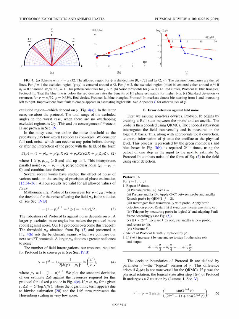
FIG. 4. (a) Scheme with γ = π/32. The allowed region for φ is divided into [0, π/2] and [π/2, π ). The decision boundaries are the redlines. For j = 1 the excluded region (gray) is centered around π/2. For j = 2, the excluded region (blue) is centered either around π/4 ifb1 = 0 or around 3π/4 if b1 = 1. This pattern continues for j > 2. (b) Noise thresholds for γ = π/32. Red circles, Protocol Ia; blue triangles,Protocol Ib. That the blue line is below the red demonstrates the benefits of FT phase estimation for higher bits. (c) Standard deviation vsresources for γ = π/32, p = 0.63%. Red circles, Protocol Ia; blue triangles, Protocol Ib; markers denote bits starting from 1 and increasingleft to right. Improvement from fault tolerance appears in estimating higher bits. See Appendix C for other values of γ .

excluded region—which depend on γ [Fig. 4(a)]. In the lattercase, we abort the protocol. The total range of the excludedangles in the worst case, when there are no overlappingexcluded regions, is 2tγ . This and the convergence of ProtocolIa are proven in Sec. IV.

In the noisy case, we define the noise threshold as theprobability p below which Protocol Ia converges. We considerfull-rank noise, which can occur at any point before, during,or after the interaction of the probe with the field, of the form

E (ρ) = (1 − p)ρ + p(pxXρX + pyXZρZX + pzZρZ ), (2)

where 1 � p, px,y,z � 0 and add up to 1. This incorporatesparallel noise (px = py = 0), perpendicular noise (pz = py =0), and combinations thereof.

Several recent works have studied the effect of noise ofvarious ranks on the scaling of precision of phase estimation[15,34–36]. All our results are valid for all allowed values ofpx,y,z.

Mathematically, Protocol Ia converges for p < pth, wherethe threshold for the noise affecting the field pth is the solutionof (see Sec. IV B)

1 − (1 − p)2t−1 = δ(γ ) = | sin γ |/2. (3)

The robustness of Protocol Ia against noise depends on γ . Alarger γ excludes more angles but makes the protocol morerobust against noise. Our FT protocols overcome this tradeoff.The threshold pth obtained from Eq. (3) and presented inFig. 4(b) sets the benchmark against which we compare ournext two FT protocols. A larger pth denotes a greater resilienceto noise.

The number of field interrogations, our resource, requiredfor Protocol Ia to converge is (see Sec. IV B)

N = (2t − 1)1

2[δ(γ ) − p f ]2ln

(2t

ε

), (4)

where p f = 1 − (1 − p)2t−1. We plot the standard deviation

of our estimate φ against the resources required for thisprotocol for a fixed p and γ in Fig. 4(c). If p pth for a givent, φ = O(log N/N ), where the logarithmic term appears dueto bitwise estimation [20] and the 1/N term represents theHeisenberg scaling in very low noise.

B. Error detection against field noise

First we assume noiseless devices. Protocol Ib begins bycreating a Bell state between the probe and an ancilla. Theprobe is then encoded using QRMCs. The encoded subsysteminterrogates the field transversally and is measured in thelogical X basis. This, along with appropriate local correction,teleports information of φ onto the ancillae at the physicallevel. This process, represented by the green rhombuses andblue boxes in Fig. 3(b), is repeated 2 j−1 times, using theoutput of one step as the input to the next to estimate bj .Protocol Ib combats noise of the form of Eq. (2) in the fieldusing error detection.

Protocol IbFor j = 1, . . . , t1. Repeat M times.

(i) Prepare probe |+〉. Set k = 1.(ii) Prepare ancilla |0〉. Apply CNOT between probe and ancilla.Encode probe by QRM(1, j + 2).(iii) Interrogate field transversally with probe. Apply errordetection on probe. Restart (i) if syndrome measurements reject.(iv) Teleport by measuring probe in logical X and adapting Pauliframe accordingly (see Fig. (5)).(v) If k < 2 j−1, increase k by one, use ancilla as new probe,and return to (ii).(vi) Measure X .

2. Step 2 of Protocol Ia with γ replaced by γ ′.3. If j �= t increase j by one and go to step 1, otherwise exit

and output

φ = b1π

2+ b2

π

4+ . . . + bt

π

2t.

The decision boundaries of Protocol Ib are defined byparameter γ ′—the “logical” version of γ . This differencearises if Rz(φ) is not transversal for the QRMCs. If γ was thephysical rotation, the logical state after step 1(iv) of ProtocolIb undergoes a Z rotation by (Lemma 1, Sec. V)

γ ′ = γ − 2 arctan

(sin(2 j+1γ )

(2 j+2 − 1) + cos(2 j+1γ )

). (5)

022335-4

FAULT-TOLERANT QUANTUM METROLOGY PHYSICAL REVIEW A 100, 022335 (2019)

FIG. 5. Steps 1(i)–1(iv) of Protocol Ib. For k = 1, |ψ〉 = |+〉or else the output of previous k. EQRM is the encoding circuit forQRM(1, j + 2), Rz(φ)L is logical (transversal) application of thefield, {SZ

i } are all the Z stabilizer measurements, and XL is logicalX measurement from which we extract the X syndromes.

For large j this nontransversality has a small effect since γ ′ =γ − O(2− j ). Following the analysis of Protocol Ia, the rangeof the excluded angles in the worst case is again 2tγ , not 2tγ ′.

The probability of logical error in a single interrogation isthe probability that the syndrome measurements do not detectthe errors and the errors corrupt X measurement. Since φ isunknown we cannot apply a suitable dephasing transformation(also known as twirl) on the noisy states to reduce noiseto only Z errors, unlike FT quantum computing [26]. Sowe measure both X and Z stabilizers and the correspond-ing failure probabilities pX

err and pZerr are given in Eqs. (19)

and (23), Sec. VI. The threshold for p is now obtained bysolving p f ≡ 1 − (1 − pX

err )2 j−1

(1 − pZerr )

2 j−1 = δ(γ ′), whichcorresponds to Eq. (3) at the logical level. This threshold ispresented in Fig. 4(b). For higher-order QRMCs, pX

err pZerr

below the threshold.The number of field interrogations, our resources, required

for Protocol Ib to converge depends on pn, the probability ofretransmission due to noise, and pr, the probability of retrans-mission due to nontransversality. Using Lemma 2, Sec. V,

pr = 1 − (1 − 12 j+1 )

( j+2)2 j−1

. If the probabilities of passing theX and Z error syndrome measurements for bit j are given bypXpass and pZpass, respectively [Eqs. (17) and (20), Sec. VI],pn = 1 − (pXpass pZpass)2 j−1

. This gives

N =t∑

j=1

2 j−1C( j)1

2[δ(γ ′) − p f ]2ln

(2t

ε

), (6)

with C( j) = (2 j+2 − 1)/(1 − pn)(1 − pr ) being the overheadfrom the QRMC. We plot φ versus the resources required—including extra interrogations due to retransmissions—for afixed p and γ in Fig. 4(c).

Now we deal with noise in devices, which we assume tobe independent of the field noise. This results in the newthreshold equation

1 − (1 − p′X

err

)2 j−1(1 − p′Z

err

)2 j−1

(1 − p′)3×2 j−1+2 = δ(γ ′) (7)

involving noise of the form of Eq. (2) for the field (p) andthe devices (p′). The failure probabilities p′X

err and p′Zerr now

have an additional contribution from the noisy devices, whichitself includes the effect of noisy nontransversal encodingand noisy syndrome measurements. The latter are EQRM and{SZ

i } and XL in Fig. 5. Since Eq. (7) involves two variablesp and p′, there is no unique solution for the two thresholds,pth and p′

th. For small p′th, see Fig. 6 for improvements in pth

and Sec. VII A for details.

FIG. 6. Relationship between thresholds pth and p′th for γ =

π/32 and j = 4. Improved threshold for Protocol Ib with devicenoise (dashed blue) over Ia (solid red/dark gray). Improved thresholdof Protocol Ic (solid green/light gray) over Protocol Ib with devicenoise in subregion enlarged. Protocol Ib without device noise (dottedblue) is provided for reference.

C. Fault tolerance everywhere

Finally, Protocol Ic [Fig. 3(c)] combats noise at any stageof the sensing process. In quantum computation, the lackof transversal universal gate sets [28] is overcome by eithergate distillation or code switching. In metrology, the for-mer is prohibitive because φ is unknown (see Sec. VII B).Our Protocol Ic proceeds via switching [37] between theQRM(1,3) Steane code which is transversal for H and higher-order QRMCs [38], along with the error detection method ofProtocol Ib.

Protocol IcFor j = 1, . . . , t1. Repeat M times.

(i) Prepare |+L〉 using FT procedure employing the Steane codeand switch to QRM(1, j + 2). Set k = 1.(ii) Prepare ancilla |0L〉 using FT procedure employingQRM(1, j + 2). Apply transversal FT CNOT between probe.and ancilla.(iii) Interrogate field transversally with probe. Apply errordetection on probe. Restart (i) if syndrome measurements reject.(iv) Teleport by measuring probe in logical X and adapting Pauliframe accordingly (see Fig. (8)).(v) If k < 2 j−1, increase k by one, use ancilla as new probe,and return to (ii).(vi) FT measurement of logical X .

2. Step 2 and 3 of Protocol Ib.

Protocol Ic behaves exactly as Protocol Ib in terms ofconvergence and resource requirements. The thresholds forProtocol Ic are given by modifying the failure probabilitiesp′X

err and p′Zerr, the number of points of failure, and the noise

p′ in Eq. (7). Protocol Ic has no non-transversal encodingand failure probabilities just include noisy syndrome mea-surements (Sec. VII C). Compared to Protocol Ib, ProtocolIc now provides a larger improvement in pth over ProtocolIa, but over a reduced range of p′ as shown in Fig. 6. Theimprovements are limited by the poor QRMC error correction

022335-5

THEODOROS KAPOURNIOTIS AND ANIMESH DATTA PHYSICAL REVIEW A 100, 022335 (2019)

thresholds. Larger improvements should be attainable if codeswith better thresholds and suitable transversality propertiescan be designed.

IV. ANALYSIS OF THE PARAMETRIZEDRUDOLPH-GROVER SCHEME: CONVERGENCE,

NOISE RESILIENCE, AND RESOURCES

The unknown phase parameter φ is expressed in a radix2 expansion as φ = 2π × 0.b0b1b2 . . . = b0

2π2 + b1

2π22 +

b22π23 . . .. Setting b0 = 0 leads to

φ = b1π

2+ b2

π

4. . . . (8)

We denote our estimate of the unknown parameter after theprotocol as φ.

A. Noiseless case

Assume first that Protocol Ia is implemented in the noise-less case. Let p1 be the probability of obtaining zero (eigen-value +1) in our measurements in a noiseless Protocol Ia forj = 1. Let p1 be our (real valued) estimate, which comes fromaveraging over M independent and identically distributedrepetitions. Seeking | p1 − p1| � δ leads to

prob(| p1 − p1| � δ) � 1 − 2e−2Mδ2

from the Hoeffding inequality.Let us choose δ = | cos2( π

4 ) − cos2( π4 − γ

2 )| =| sin(γ )/2|. For γ = π/8, δ ≈ 0.191; for γ = π/32,δ ≈ 0.049. This implies the following, for angle φ in theallowed region [0, π/2 − γ ] or [π/2 + γ , π ].

(i) If 0 � φ1 < (π/2 − γ ),

prob(

0 � φ <π

2

)� 1 − 2e−2Mδ2

(9)

and prob(b1 = b1 = 0) is equally high.(ii) If (π/2 + γ ) < φ1 � π,

prob(π

2� φ < π

)� 1 − 2e−2Mδ2

and prob(b1 = b1 = 1) is equally high.This concludes the analysis for j = 1.Assuming that the estimation for j = 1 was correct,

we proceed to the estimation of the other bits. We useinduction to calculate all the conditional probabilities.Suppose all bits bk , k < j are correctly estimated. Theprobe after the 2 j−1 consecutive interrogations is (|0〉 +eiφ j |1〉)/

√2, where φ j = 2 j−1φ = 2π × 0.b j−1b jb j+1 . . . =

b j−12π2 + b j

2π22 + b j+1

2π23 . . ., where b j−1 is known from pre-

vious estimation.Again, using the Hoeffding inequality, we bound the prob-

ability of having error smaller than the same parameter δ. Theallowed region for φ j − b j−1π should be again [0, π/2 − γ ]or [π/2 + γ , π ], and the following hold.

(i) If b j−1π � φ j < b j−1π + (π/2 − γ ),

prob(

0 � φ j − b j−1π <π

2

)� 1 − 2e−2Mδ2

and prob(b j = b j = 0) is equally high, conditioned on theestimations of prior bits being correct.

(ii) If b j−1π + (π/2 + γ ) � φ j � b j−1π + π ,

prob(π

2� φ j − b j−1π < π

)� 1 − 2e−2Mδ2

and prob(b j = b j = 1) is equally high, conditioned on theestimations of prior bits being correct.

This concludes our analysis for j.The probability that all the bits up to bt are estimated cor-

rectly is lower bounded by (1 − 2e−2Mδ2)t � 1 − 2te−2Mδ2

. Tohave a maximum error ε in our estimator to be correct up tothe t th bit, we choose M such that ε � 2te−2Mδ2

. This leads to

M � 1

2δ2ln

(2t

ε

). (10)

The total overhead in uses of the field to estimate φ to t bitswith error ε becomes

N = 2t − 1

2δ2ln

(2t

ε

). (11)

The allowed angles for which the above convergencearguments hold are as follows. From the analysis above,the estimation of the first bit converges with high proba-bility if φ ∈ [0, π/2 − γ ] ∪ [π/2 + γ , π ]. Thus the lengthof the excluded region is 2γ . For the second bit, considerestimating φ2 = 2φ. If b1 = 0, φ ∈ [0, π/4 − γ /2] ∪ [π/4 +γ /2, π/2], and, if b1 = 1, φ ∈ [π/2, π/2 + π/4 − γ /2] ∪[π/2 + π/4 + γ /2, π ]. The length of the excluded region isagain 2γ .

In general, consider estimating φ j = 2 j−1φ mod 2π.

Suppose b1 = . . . = b j−2 = 0. If b j−1 = 0,

φ ∈[0,

π

2 j− γ

2 j−1

]∪

[ π

2 j+ γ

2 j−1,

π

2 j−1

],

and, if b j−1 = 1,

φ ∈[ π

2 j−1,

π

2 j−1+ π

2 j− γ

2 j−1

]∪

[ π

2 j−1+ π

2 j+ γ

2 j−1,

π

2 j−2

].

Continuing with the 2 j−2 possibilities for b1, . . . , b j−2, eachof which excludes regions of length γ /2 j−2, we obtain atotal excluded region of length 2γ . In the worst case, of theregions not being overlapping, the excluded region has totalangle 2tγ .

B. Noisy case

We now consider the noisy case and denote the probabilityof an error occurring in an interrogation step as p. Then, theprobability p f (p, j) of the measurement result being incorrectafter a number of interrogations and a final measurementdepends on p and the number of interrogations (which de-pends on j). In Protocol Ia, we undertake 2 j−1 interrogations,whereby p f is upper bounded by 1 − (1 − p)2 j−1

.The following analysis holds for any j. Let pj be the

probability of obtaining zero (eigenvalue +1) if there was nonoise. With probability p f , this result we get will be flipped.Let p′

j be the “noisy” probability of obtaining zero. Then

p′j = p j (1 − p f ) + (1 − p j )p f , (12)

whereby p′j − p j = p f (1 − 2p j ), implying

|p′j − p j | � p f . (13)

022335-6

FAULT-TOLERANT QUANTUM METROLOGY PHYSICAL REVIEW A 100, 022335 (2019)

After M repetitions, the Hoeffding inequality gives the noisyestimate p′

j as

prob(| p ′j − p′

j | � δ) � 2e−2Mδ2. (14)

Adding |p′j − p j | gives

prob(| p ′j − p′

j | + |p′j − p j | � δ + |p′

j − p j |) � 2e−2Mδ2.

We then use the fact that [prob(x � b) � c] ∧ (y � x) ⇒prob(y � b) � c, which can be proven by writing the proba-bilities as integrals and changing variables. Since | p ′

j − p j | �| p ′

j − p′j | + |p′

j − p j |,prob(| p ′

j − p j | � δ + |p′j − p j |) � 2e−2Mδ2

.

Thus,

prob(| p ′j − p j | � δ) � 2e−2M(δ−|p′

j−p j |)2 � 2e−2M(δ−p f )2,

whereby

prob(| p ′j − p j | < δ) > 1 − 2e−2M(δ−p f )2

.

We therefore get confidence in our estimation for the jth bitonly if p f < δ, in which case the same proof of convergenceholds as in the noiseless case. This means that there is aprobability p of failure in a single interrogation above whichthe protocol does not converge and is given by the solution of1 − (1 − p)2t−1 = δ = | cos2( π

4 ) − cos2( π4 − γ

2 )| for a fixed γ

and t . We call this the noise threshold pth of the protocol.Following the same analysis as before and replacing δ by

δ − p f (p, t ) we have

N = 2t − 1

2(δ − p f )2ln

(2t

ε

).

Standard deviation

A canonical way of quantifying the performance of anestimator is its standard deviation φ. We derive this fora fixed ε adapting the technique from Ref. [16]. At theconclusion of the estimation protocol, with probability 1 − ε

an estimate φest is obtained which is the correct one up to t bitsof precision (φest � π/2t+1). Otherwise, we get a randomestimate φr, which we assume to be independent of φest toease our analysis. Thus φ = (1 − ε)φest + εφr, and

φ =√

(1 − ε)2(φest )2 + ε2(φr )2

=√

(1 − ε)2π2

22(t+1)+ ε2π2.

We choose ε so that φ decreases inversely with the largestpossible function of the total overhead. Let ε = 1/2t . Sinceφ = O(2−t ) for noise significantly smaller than the thresh-old, N = O(t2t ), and we have φ = O(log N/N ), ignoringterms logarithmic in t .

V. NONTRANSVERSALITY EFFECTS IN QRMCs

We provide results for QRMCs for the effect of applyingtransversally gates that are nontransversal for a particularQRMC, under postselection for the correct syndrome out-comes. The equations for bit j in our protocols are obtainedby setting m = j + 2 in the following lemmas.

Lemma 1. Apply Rz(−φ) transversally, where φ =0.b0b1b2 . . ., on a logical single qubit state encoded by codeQRM(1, m). Postselecting on accepting the syndromes cre-ates, up to a global phase, a logical rotation of

φ′ = φ − 2 arctan

(sin(φm)

(2m − 1) + cos(φm)

), (15)

around the Z axis, where φm = 2m−1φ = 2π ×0.bm−1bmbm+1 . . . .

Proof. Let

P+1 =2m−m−2∏

i=1

(I + SZ

i

)22m−m−2

m∏i=1

(I + SX

i

)2m

(16)

be the projector to the code space, i.e., the positive eigenspaceof the Z and the X syndrome measurements SZ

i andSX

i , respectively. The effect of applying Rz(−φ) transver-sally and projecting to P+1 on logical state |0L〉 leads toP+1Rz(−φ)⊗2m−1|0L〉, which is

1√2m

P+1

⎛⎝|0〉 + e−i2m−1φ∑

x∈RM\{0}|x〉

⎞⎠.

The projections coming from the Z stabilizer measurementshave no effect on the state. The elements SX

i correspond to thegenerators of the RM code (by replacing the ones with X ’s andthe zeros with I’s) and therefore

∏mi=1(I + SX

i ) gives a sumover stabilizers that correspond to all x ∈ RM. When appliedto the above state they map each codeword to the sum of allcodewords in the code and therefore create the same (global)phase:

1 + (2m − 1)e−iφm = 1 + (2m − 1) cos φm + i(2m − 1) sin φm

where φm = 2m−1φ. Similarly for the logical |1L〉 state, we getP+1Rz(−φ)⊗2m−1|1L〉:

1√2m

P+1

⎛⎝e−i(2m−1)φ|1〉 + e−i(2m−1−1)φ∑

x∈RM

|x + 1〉⎞⎠.

Again, the projectors from the X measurements mix all thephases, leading to a global phase of

e−i(2m−1)φ + (2m − 1)e−i(φm−φ).

Therefore the whole operation adds between the computa-tional basis states a relative phase of

φ′ = arctan

((2m − 1) sin φm

1 + (2m − 1) cos φm

)− arctan

(sin[(2m − 1)φ] + (2m − 1) sin(φm − φ)

cos[(2m − 1)φ] + (2m − 1) cos(φm − φ)

),

from which Eq. (15) emerges via trigonometry. �The cost of postselection for rotations that are not transver-

sal for QRM(1, m) is given below.Lemma 2. The probability of failure in any of the SX

isyndrome measurements on a QRM(1, m)-encoded state, onwhich transversal Rz(−φ) has been applied, is less than orequal to 1 − (1 − 1

2m−1 )m

.

022335-7

THEODOROS KAPOURNIOTIS AND ANIMESH DATTA PHYSICAL REVIEW A 100, 022335 (2019)

Proof. The probability of failure in the postselection ofeach of the m syndromes is at most 1

2m−1 , for any real rotation.This comes from calculating the probability of getting resultzero in measurement i. This is given by

pi = 〈χi−1| I + SXi

2|χi−1〉 = 1

2+ 〈χi−1|SX

i |χi−1〉2

� 1

2+ 2m+1 − 8

2 × 2m+1= 1 − 1

2m−1

for |χi−1〉 being the state that comes after syndrome measure-ment i − 1 (renormalized) and |χ0〉 = Rz(−φ)⊗2m−1(|0L〉 +eiψ |1L〉)/

√2, for some ψ . The key observation here is that

SXi |χi−1〉 is a permutation of the sums of kets of |χi−1〉, where

each sum of kets comes from applying∏i−1

j=1(I + SXj ) on

each ket of the initial state |χ0〉 when written in the physicalrepresentation.

The probability of failure of all the m X syndromes—X syndromes are the only ones that potentially reject—istherefore 1 − (1 − 1

2m−1 )m. This creates an extra overhead inthe resource count. �

VI. PROTOCOL Ib WITH NOISELESS DEVICES: ERRORDETECTION FAILURE PROBABILITIES

In order to calculate the thresholds and resources of Proto-col Ib we need to find the probability that the error detectionprocedure fails at each step k. We exploit the idea of onlyerror detecting for the errors, followed by the decoding of thecode subspace to a Hilbert space of one qubit, in order to getimproved thresholds [39]. An instance of the circuit used forerror detection at each step k of Protocol Ib (Fig. 5) is givenfor m = 4 in Fig. 7.

For Protocol Ib, unlike in magic state distillation in quan-tum computing (for more details see Ref. [40]), the circuitof Fig. 7 is applied on a physical level. In Protocol Ib errorsonly enter through the Rz(φ) gates and of the form of Eq. (2).Rejections after the syndrome measurements can happen ei-ther because of noise or because of the nontransversal effectsanalyzed in Sec. V. There is no dependency between the twosources of rejection and thus we restrict our analysis here torejections due to noise.

Failure comes when the logical outcome of the X measure-ment is flipped in the case that no syndrome error is beingdetected. The failure probabilities at the syndrome detectionfor X or Z errors, pX

err and pZerr, respectively, are

pXerr = p(error|X pass) = p(error, X pass)

p(X pass)

and, similarly,

pZerr = p(error|Z pass) = p(error, Z pass)

p(Z pass).

First we focus on the stabilizers that detect the Pauli Xerrors. These correspond to the rows of the parity checkmatrix Hz of the RM∗ code. The undetected noise operatorscorrespond to the codewords of the RM∗ code, includingthe noiseless case which corresponds to zero, given by V ⊥

Hz.

FIG. 7. FT application of transversal Rz(φ) using QRM(1,4) andteleportation onto input state |ψ〉.

Thus,

p(X pass) = WV ⊥Hz

(1 − p, p), (17)

where WV (x, y) = ∑c∈V xn−wt(c)ywt(c) is the weight polyno-

mial of V ∈ GF(2n) and wt(c) is the number of ones in thecodeword c. We can then write the probability of retransmis-sion due to Pauli X noise as pX

n = 1 − WV ⊥Hz

(1 − p, p).The above undetected operators could potentially corrupt

the logical X measurement if they happen either before orduring the application of the Rz(φ) signal. To understand thiswe represent the signal plus noise operation as Rz(θ )XRz(φ −θ ) for some angle θ � φ. Up to global phase this is equal toRz(2θ )XRz(φ), thus equal to the original signal plus a PauliX that has no effect on the logical X measurement, plus anextra term Rz(2θ ) that can corrupt the logical X measurementwhen θ �= 0. From discretization of errors (Ref. [21], Theorem10.2) and the fact that QRMCs can recover from Z noise,these non-Pauli errors Rz(2θ ) are detected by the X stabilizermeasurements unless they correspond to codewords of theHamming code, and the latter corrupt the logical measurementonly when they have odd parity. Since the weights of thecodewords that are excluded by these refinements are large,their contribution in the error probability is negligible andtherefore we can include in our calculation all codewords ofthe RM∗ code except identity. Therefore,

pXerr =

WV ⊥Hz

(1 − p, p) − (1 − p)2m−1

WV ⊥Hz

(1 − p, p). (18)

022335-8

FAULT-TOLERANT QUANTUM METROLOGY PHYSICAL REVIEW A 100, 022335 (2019)

Using the codeword weights of RM∗ from Appendix A, we obtain

pXerr = (2m − 1)(1 − p)2m−1

p2m−1−1 + (2m − 1)(1 − p)2m−1−1 p2m−1 + p2m−1

(1 − p)2m−1 + (2m − 1)(1 − p)2m−1 p2m−1−1 + (2m − 1)(1 − p)2m−1−1 p2m−1 + p2m−1. (19)

The results for bit j are obtained by setting m = j + 2. Giventhe form of noise of Eq. (2) and that X error detection ismade first, the single qubit X error probability is p(px + py).However, since the function in Eq. (19) is monotonicallyincreasing in p, we can replace p(px + py) by p and get anupper bound ∀ px, py.

The stabilizers that detect the Pauli Z errors correspond tothe rows of the parity check matrix Hx of the dual of the RMcode, which is the Hamming code (2m − 1, 2m − 1 − m, 3).The undetected noise operators correspond to the codewordsof the Hamming code, including the noiseless case whichcorresponds to zero, given by V ⊥

Hx. Thus,

p(Z pass) = WV ⊥Hx

(1 − p, p) (20)

and the probability of retransmission due to Pauli Z noise ispZ

n = 1 − WV ⊥Hx

(1 − p, p).The subset of undetected operators that lead to an er-

ror in the logical X measurement consists of those which

anticommute with the tensor product of X operators: theones with odd parity. From duality, the parity matrix HRM

of the RM code is the generator of the codewords of theHamming code. The subset of odd codewords is obtained bycomplementing the code generated by the parity check matrixHz of RM∗, which is the same as HRM without the 1 row, thuskeeping only its even generators. Thus,

pZerr = WVHz

(p, 1 − p)

WV ⊥Hx

(1 − p, p), (21)

Using the MacWilliams identity WV (x, y) = 1|V |WV ⊥ (x +

y, x − y), we obtain

pZerr =

∣∣VHx

∣∣WV ⊥Hz

(1, 2p − 1)∣∣VHz

∣∣WVHx(1, 1 − 2p)

. (22)

Using the codeword weights of RM∗ and RM fromAppendix A and |VHx |/|VHz | = 2m/2m+1 = 1/2, we obtain

pZerr = 1 + (2m − 1)(2p − 1)2m−1−1 + (2m − 1)(2p − 1)2m−1 + (2p − 1)2m−1

2[1 + (2m − 1)(1 − 2p)2m−1 ]. (23)

Again, the above is an upper bound on the failure probabil-ity due to Z errors, when noise is of the form of Eq. (2), for allvalues of pz.

VII. NOISY DEVICES

A. Protocol Ib: Noisy device thresholds

If we assume noisy devices in Protocol Ib, by allowing anydevice to have noise of the form of Eq. (2) with probabilityp replaced by the device noise probability p′, the thresholdcalculation is different. Failure probabilities of the detectionprocedure for X and Z errors are denoted by p′X

err and p′Zerr,

respectively. These probabilities are given by replacing prob-ability p by p + devIb(p′) in Eqs. (19) and (23), respectively.Probability devIb(p′) captures the effect of all device noise[except for state preparation and CNOT error, which are in-cluded separately in the last term on the left-hand side ofEq. (26)] on one qubit in the detection procedure and is givenby

devIb(p′) = [ce + (2m − m − 2) + 1]p′ (24)

where ce is the number of points of failure in the nontransver-sal encoding procedure EQRM that affect one qubit. The oper-ations in the encoding procedure correspond to the generatormatrix of RM∗(1, m). On average, there are approximately(m + 1)2m−1/(2m − 1) points per qubit where the entanglingoperations apply on the particular qubit. Since each entanglingoperation in the coding involves approximately 2m−1 qubits,

we have

〈ce〉 ≈ (m + 1)2m−1

2m − 12m−1. (25)

For our protocol, we need to set m = j + 2 in the previoustwo equations.

The failure probability at the output of Protocol Ib withdevice noise is bounded away from 1 by the joint probabilitythat in all of the 2 j−1 rounds both the state preparation andCNOT are correct and the detection procedure does not fail.The latter joint probability can be written as the product ofthe probability of correct state preparation or CNOT and theprobability of detection not failing conditioned on correctstate preparation or CNOT. The points of failure for state prepa-ration or CNOT are 3 × 2 j−1 + 2. This includes initial probepreparation and Hadamard, as well as ancilla preparation andCNOT (two points of failure) at each interrogation step. Noticethat performing the teleportation correction can be avoidedby updating the Pauli frame. Then the threshold equationbecomes

1 − (1 − p′X

err

)2 j−1(1 − p′Z

err

)2 j−1

(1 − p′)3×2 j−1+2 = δ(γ ′). (26)

Since Eq. (26) involves two variables p and p′, there is nounique solution but rather a relation for the two thresholds—pth and p′

th—as depicted in Fig. 6.

B. Protocol Ic: Why code switching?

In Protocol Ic we combat noise that can enter at any stageof the phase estimation protocol, in interrogating the field, as

022335-9

THEODOROS KAPOURNIOTIS AND ANIMESH DATTA PHYSICAL REVIEW A 100, 022335 (2019)

well as probe and ancilla preparation, entangling gates, andmeasurements.

As in quantum computing, we need to employ some ex-tra encoding throughout the protocol. If we use transversalquantum codes, the same encoding cannot be used everywheresince there is no quantum code transversal for a universal setof gates [28]. Two techniques are known to solve this issue:gate (or state) distillation and code switching. First we explainwhy the first technique is prohibitively expensive in terms ofour resources for phase estimation.

1. Gate distillation

Everything is performed on an underlying quantum errorcorrecting code which is transversal only for Clifford oper-ations, e.g., QRM(1,3), also known as the Steane code. Thenon-Clifford operations are performed by injecting into thiscode special states, sometimes called magic states, and thenapplying a distillation procedure using a higher-order QRMCto reduce their noise [26].

In our case, the non-Clifford part of the computation isthe Rz(φ) rotation. In metrology, however, φ is unknown.Similarly to Ref. [26], we could inject a state on whichthe Rz(φ) rotation has been applied and teleport it into therest of distillation circuit using the teleportation circuit ofFig. 2. The distillation would then proceed accounting fordiscretization effects as described in Sec. V. However, in orderfor teleportation to succeed, after the logical measurement ofthe first qubit a logical correction on the second needs to beapplied:

Rz(φ)XR†z (φ) ∝ Rz(2φ)X, (27)

where proportionality captures an irrelevant global phase.In quantum computing, commonly φ = π/2n and Rz(φ)

belongs to the nth level of the Clifford hierarchy. Then,Rz(2φ) belongs to the (n − 1)th level and thus injecting,distilling, and teleporting more magic states to implementthe corrections is a terminating process, with the number ofsteps depending on n (see Refs. [41,42] for more details).For metrology φ ∈ [0, π ] and therefore a similar procedureis not guaranteed to terminate. This, on its own, is not amajor issue since we could postselect on measuring zeroafter k consecutive teleportations with the probability of 1being exponentially small on k (teleportation measurementsare unbiased). The problem is that distilling a Rz(2kφ) rota-tion, for unknown φ, means interrogating the field with thesame state 2k times, which will introduce noise of strength2k p. Even for k = 2, the thresholds we have calculated forthe field noise (Protocol Ib) will be worse than the non-FTcase (Protocol Ia). Thus, the unknown nature of the rotation,which necessitates using the same field multiple times for theteleportation corrections, means that gate distillation is notgiving a benefit over the non-FT protocol.

One could avoid any correction by applying postselectionon the very first teleportation step. This leads the failure prob-ability of one Rz(φ) application in the distillation circuit to be1/2. Since the distillation circuit uses QRMCs of block sizes2 j+2 − 1 the failure probability of transversal application onRz(φ) on the block is 1 − (1/2)2 j+2−1. For 2 j−1 interrogationsthis amounts to 1 − (1/2)2 j−1(2 j+2−1), adding an extra double

|ψL〉 / • / FT M. Recov. Rz(φ) {SZi } X

|0L〉 / / FT M. Recov.

FIG. 8. Protocol Ic circuit. Operations CNOT, Rz(φ), and Xmeasurement are all transversal. Operations {SZ

i } represent all Zstabilizer measurements. Fault-tolerant measurements and recoveryrequire extra ancillae and correct up to one error.

exponential term in the resource count C( j) from the code.This would be prohibitive.

2. Code switching

We thus resort to the alternative technique of code switch-ing [37,38]. Here, the state is encoded throughout the protocolwith a quantum code but is not the same at every stage. Codeswitching exploits the fact that different members of QRMCsare transversal for different gate sets and one can switch be-tween those codes using ancilla qubits and FT measurements.In Protocol Ic we start with a state |0〉 encoded (by meansof FT measurements) by the Steane code and fault tolerantlyapply a Hadamard gate in order to prepare the |+L〉 probestate. Then we switch to the QRM(1, m) for m = j + 2 onwhich we apply the rest of the protocol.

The circuit applied for each interrogation, Fig. 8, is similarto that of Protocol Ib (Fig. 5). The difference is that the inputstate |ψ〉 is already encoded with the required QRMC andtherefore the nontransversal operation EQRM is not needed.The state is entangled by means of a transversal CNOT gatewith the ancilla qubit which is also fault-tolerantly encodedwith the same QRM(1, m) code. At every step we apply FTsyndrome measurements and recovery operations in the samefashion it is applied in quantum computing [21], the failureprobability of which is given in Sec. VII D. The overhead thatcomes from the QRM encoding and switching is not countedsince we count as a resource the number of uses of the field,which is the same as in Protocol Ib.

C. Protocol Ic: Noisy device thresholds

Similarly to Sec. VII A, we calculate how the noise in de-vices affects the error thresholds of Protocol Ic. There are twodifferences from Protocol Ib. First, the encoding procedure forthe QRMCs is now done during the preparation of the probeand ancillae and is fault tolerant. Second, after every operationa round of fault-tolerant error correction is applied. The failureprobability of the error correction procedure is denoted bypEC and given in Sec. VII D. The failure probabilities of thedetection procedure are denoted p′′X

err and p′′Zerr and given by

replacing probability p by p + devIc(p′) in Eqs. (19) and (23),respectively, where

devIc(p′) = [3 × 2m + 1 + (2m − m − 2) + 1]p′. (28)

This includes the errors on one qubit from previous syn-drome measurements and recovery plus the errors in the error

022335-10

FAULT-TOLERANT QUANTUM METROLOGY PHYSICAL REVIEW A 100, 022335 (2019)

detection syndrome measurements. For our protocol, we needto set m = j + 2 in the above equation.

Now, the number of FT measurement and recovery stepsis 3 × 2 j−1 + j + 1. This includes FT probe preparation, FTHadamard and j − 1 steps of switching to QRM(1, j + 2),as well as FT ancilla preparation and FT CNOT (two steps)at each interrogation step. We conservatively approximate thesuccess probability of FT probe preparation, FT Hadamard,and each FT switching step by the success probability of FTmeasurement and the recovery step of QRM(1, j + 2). Thenthe threshold equation becomes

1 − (1 − p′′X

err

)2 j−1(1 − p′′Z

err

)2 j−1

(1 − pEC)3×2 j−1+ j+1 =δ(γ ′).

(29)

The solution involves two variables and is depicted in Fig. 6.We observe that the range of values of p′

th in which pth isimproved over Protocol Ia is smaller than in Protocol Ib withdevice noise, but, within this region, there is a subregionwhere Protocol Ic gives higher thresholds than Protocol Ib.This improvement, however, is small and the reason for thisis the large amount of operations involved in QRMC errorcorrection.

D. Failure probabilities of QRMCs as error-correcting codes

To analyze the thresholds of Protocol Ic we calculate thefailure probability of the error correction procedure usingQRMCs.

Since QRMCs can correct one error of any type, the noisethreshold comes from the probability of having two or moreerrors during all possible operations between two rounds offault tolerance. The approximate thresholds for QRM(1,3)are provided in Ref. [21]. We follow the same techniques tocalculate approximate thresholds for QRM(1, m) for m > 3.

We begin by enumerating the combinations leading to twoerrors at the output. We consider the FT measurement andrecovery operation on the first logical qubit immediately afterthe application of transversal CNOT in Fig. 8. The number ofways two errors can occur at the output of the first logicalqubit is listed below.

(i) Two errors at the previous syndrome measurement andrecovery operations. Since there are two blocks with c0 = 3 ×2 × m × 2m−1 + 2m − 1 points of failure in each, this numberis c2

0.(ii) One error at the previous syndrome measurement and

recovery operations at one of the two blocks, and anotherduring the logical two qubit gate. This number is 2c0(2m − 1).

(iii) Both during the logical two qubit gate. This number is(2(2m − 1)

2 ).(iv) Two errors due to incorrect syndrome measurement.

This number is (2m)(2 × 2m−1 )2 ).

(v) Both at the syndrome measurements: c20.

(vi) One at the syndrome measurement and another duringrecovery: c0(2m − 1).

(vii) Both during recovery: (2m − 1)2.Summing all the above contributions, we get

c = 2c20 +

(2(2m − 1)

2

)+ (2m)

(2m

2

)+ 3c0(2m − 1)

+(2m − 1)2.

|0〉 H • · · · • Rz(φ) • · · · • H Z

|0〉 · · · Rz(φ) · · ·

|0〉 · · · Rz(φ) · · ·

FIG. 9. Parallel phase estimation without fault tolerance.

The probability of failure of the error correction procedure,which is the probability of having at least two errors, is then

pEC ≈ cp′2, (30)

where p′ is the probability of a single component in the devicebeing affected by noise.

VIII. PARALLEL PROTOCOLS

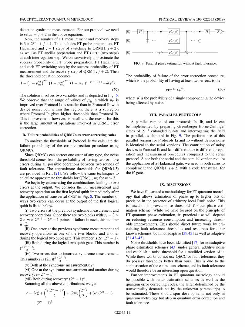
A parallel version of our protocols Ia, Ib, and Ic canbe implemented by preparing Greenberger-Horne-Zeilingerstates of 2 j−1 entangled qubits and interrogating the fieldin parallel, as depicted in Fig. 9. The performance of thisparallel version for Protocols Ia and Ib without device noiseis identical to the serial versions. The contribution of noisydevices in Protocol Ib and Ic is different due to different prepa-ration and measurement procedures compared to the serialprotocol. Since both the serial and the parallel version requirethe application of a Hadamard gate, we need in both cases tocomplement the QRM(1, j + 2) with a code transversal forthe H gate.

IX. DISCUSSIONS

We have illustrated a methodology for FT quantum metrol-ogy that allows estimation of phase up to higher bits ofprecision in the presence of arbitrary local Pauli noise. Thisis based on improved noise thresholds for our phase esti-mation scheme. While we have focused on the principle ofFT quantum phase estimation, its practical use will dependon reducing resource consumption and increasing thresh-olds improvements. This should direct future work by cal-culating fault tolerance thresholds and resources for otherknown schemes, both nonadaptive [39,43] as well as adaptive[21,43–45].

Noise thresholds have been identified [17] for nonadaptivephase estimation schemes [43] under general additive noiseand establish a noise threshold for a modified version of it.While these works do not use QECC or fault tolerance, theydo possess thresholds better than ours. This is due to thesophistication of the estimation scheme, and its fault tolerancewould therefore be an interesting open question.

Further improvements in FT quantum metrology shouldbe possible with better estimation schemes as well as thequantum error correcting codes, the latter determined by thetransversality demands set by the unknown parameter(s) tobe estimated. These should spur developments not only inquantum metrology but also in quantum error correction andfault tolerance.

022335-11

THEODOROS KAPOURNIOTIS AND ANIMESH DATTA PHYSICAL REVIEW A 100, 022335 (2019)

ACKNOWLEDGMENTS

We thank T. Rudolph for communications about Ref. [20],B. Terhal for pointing us to Ref. [17], D. Branford fortechnical discussions, J. Friel for commenting on the pa-per, and S. Ferracin for graphics assistance. This work waspartly supported by the UK Engineering and Physical Sci-ences Research Council (Grant No. EP/K04057X/2) and theUK National Quantum Technologies program (Grants No.EP/M013243/1 and No. EP/M01326X/1).

APPENDIX A: QUANTUM ERROR CORRECTION

It is known [23] that transversal gates on stabilizer codesare necessarily at a finite level of the Clifford hierarchy [46].This is based on the notion of disjointness, which is a metricof stabilizer quantum error-correcting codes and is, roughlyspeaking, the number of mostly nonoverlapping representa-tives of any given nontrivial logical Pauli operator.

Theorem 1 (Theorem 5 in Ref. [23]). Consider a stabilizercode with minimum distance d↓, maximum distance d↑, anddisjointness . If M is an integer satisfying

d↑ < d↓M−1,

then all transversal logical operators are in the Mth level of theClifford hierarchy CM .

This theorem implies that in our construction for FTmetrology we cannot hope to use a stabilizer code that istransversal for any gate Rz(φ) for φ ∈ R.

1. Reed-Muller codes

Reed-Muller codes RM(r, m) of block length n = 2m, for0 � r � m, dimension

∑ri=0 (m

i ), and distance 2m−r are afamily of classical block codes [31]. Reed-Muller codes havegeometric properties that allow for easy decoding. Codewordsof RM(r, m) correspond to all Boolean functions f of mvariables of degree r. Each codeword is the last column of thetruth table of f , i.e., the values of f for all different inputs. Forexample, the rows of the generator matrix of RM(1,3) containthe values of a01 + a1x1 + a2x2 + a3x3, where 1 stands for thevector of all ones, for all xi’s and each row corresponds to adifferent element of a basis on ai’s:

G =

⎡⎢⎢⎢⎣0 0 0 0 1 1 1 1

0 0 1 1 0 0 1 1

0 1 0 1 0 1 0 1

1 1 1 1 1 1 1 1

⎤⎥⎥⎥⎦.

We are interested in the divisibility properties of Reed-Muller codes, which have implications for the transversalityof the quantum Reed-Muller codes. A classical code C iscalled divisible by if divides the weight of all x ∈ C. Acode is called divisible if it is divisible by > 1. First-orderRM codes are divisible by 2m−1 because exactly half of theoutputs of a boolean function of degree 1 have value 1, exceptfunction 1, which always has output 1.

QRMCs use codes constructed from RM codes. We presenttheir divisibility properties and weight distribution. The short-ened RM code, denoted by RM, is taken by keeping onlythe codewords which begin with zero and deleting their first

coordinate. Codewords of RM(1, m) can be defined by thefollowing recursive process. For m = 2,

S2 =

⎡⎢⎢⎢⎣0 0 0

0 1 1

1 0 1

1 1 0

⎤⎥⎥⎥⎦,

and for higher values of m

Sm =[Sm−1 0 Sm−1

Sm−1 1 Sm−1

].

Code RM(1, m) therefore has one codeword of weight zeroand 2m − 1 of weight 2m−1.

The punctured Reed-Muller code RM∗ is obtained byadding the 1 row to the generator of RM. RM∗ therefore hasone codeword of weight zero, 2m − 1 of weight 2m−1 − 1,2m − 1 of weight 2m−1, and one of weight 2m − 1.

2. Quantum Reed-Muller codes

A quantum Reed-Muller code QRM(1,m) is a CSS codebased on classical Reed-Muller codes. It is constructed usingthe punctured Reed-Muller code RM∗ and its even subcodeRM with logical states |x〉L ≡ ∑

y∈RM |y + x1〉, for x ∈ {0, 1}.The size of the block is 2m − 1 qubits. The minimum distanceis 3, which is the minimum distance of the dual of the RM thatis used to correct the Z errors [47].

Using the following lemma, we justify our choice ofQRM(r, m) code with r = 1 and m chosen according totransversality requirements.

Lemma 3 (Corollary 4 in Ref. [48]). Let QRM(r, m)be created by the construction described above, where 0 <

r � �m/2�. Then it is an [n = 2m − 1, 1, d = min(2m−r −1, 2r+1 − 1)] code, with transversal Tt for t = �m/r� − 1.

We can thus calculate the failure probability for QRM(r, m)with r = 1 and for r > 1 with a fixed m/r ratio, to havethe same transversality property, with an error model whereeach physical qubit is corrupted with probability 0 � p 1.We calculated the thresholds for r = 2, using the followingtheorem.

FIG. 10. Estimator of Protocol II. There are three regions:[0, π/2], [π/3, 2π/3], and [π/2, π ]. The decision boundaries forj = 1 are the red lines. There are no excluded regions.

022335-12

FAULT-TOLERANT QUANTUM METROLOGY PHYSICAL REVIEW A 100, 022335 (2019)

log log log

FIG. 11. Interrogation noise thresholds. Red circles, Protocol Ia; blue triangles, Protocol Ib without device noise. For the effect of devicenoise see Fig. 6.

Theorem 2 (Theorem 8, Chap. 15, in Ref. [31]). LetAi be the number of codewords of weight i in RM(2, m).Then Ai = 0 unless i = 2m−1 or i = 2m−1 ± 2m−1−h for someh, 0 � h � �m

2 �. Also, A0 = A2m = 1 and A2m−1±2m−1−h =2h(h+1) (2m−1)(2m−1−1)...(2m−2h+1−1)

(22h−1)(22h−2−1)...(22−1) . Finally, A2m−1 = 21+m+(m2 ) −∑

i �=2m−1 Ai.We use the technique of Sec. VI to calculate the thresholds.

We find the thresholds for r = 2 with the same transversalproperties worse than the case r = 1. Given that the thresholdcalculations for � 3 are too prolix and the block sizes toolarge, we choose r = 1.

Transversality of QRM(1,m) is based on the fact thatall the codewords of RM are divisible by = 2m−1, whiletheir complement is divisible by = 2m−1 − 1 or 2m − 1.Transversality enables different operations on each logicalcomputational basis-state modulo 2m−1, by applying transver-sal gates on the 2m − 1 physical qubits. In particular, applyingtransversal Tn on QRM(1, n + 1) will apply the logical T †

ngate. For example, QRM(1,4) is transversal for T3 = T , alsoknown as the phase-π/8 gate, but not for smaller fractions ofrotations around the Z axis.

APPENDIX B: MIXED RADIX EXTENSIONOF THE RG ESTIMATOR

The RG estimator [20] only converges if the phase φ lies incertain regions as detailed in Sec. IV. This limitation can beovercome by slightly modifying the estimator [49]. It begins

by expressing the parameter in a mixed base as

φ = v1π

r1+ v2

π

r1r2+ v3

π

r1r2r3. . . , (B1)

where ri ∈ {2, 3}. In order to estimate dit j the qubit |+〉state interrogates the field an appropriate number of timesfollowed by a Pauli X measurement. The protocol is identicalto that depicted in Fig. 3, only with a different number ofconsecutive interrogations. Unlike Protocol Ia, Protocol IIbelow converges for all values of φ, since there is no excludedregion (Fig. 10).

Protocol II: Extended RG estimator [52]For j = 1, . . . , t1. Repeat M times.

(i) Prepare |+}.(ii) Interrogate field

∏ j−1l=0 rl times (r0 = 1).

(iii) Measure X .2. Calculate p j as the fraction of the +1 measurement outcomes

out of M. If v j−1 = 0 set φ j = cos−1(2 p j − 1) in [0, π ],or else in [π, 2π ].(i) If v j−1π � φ j < v j−1π + 5π

12 , set v j = 0 and r j = 2.(ii) If v j−1π + 5π

12 � φ j < v j−1π + 7π

12 , set v j = 1 and r j = 3.(iii) If v j−1π + 7π

12 � φ j � v j−1π + π , set v j = 1 and r j = 2.3. If j �= t add one to j and go to step 1, otherwise exit and output

φ = v1π

r1+ v2

π

r1r2. . . .

The convergence of the noiseless protocol is proven in [49].Here we discuss its noise resilience following the analysis forthe noisy Protocol Ia in Sec. IV.

log

log

log log

loglog

FIG. 12. Precision as a function of the number of interrogations, our resource. Red circles, Protocol Ia; blue triangles, Protocol Ib withoutdevice noise; markers denote bits. Improvement from fault tolerance is illustrated in estimating higher bits. Noise chosen at the noise thresholdsof Protocol Ia which are closer to 0.63%: (a) p = 0.639%, (b) p = 0.626%, and (c) p = 0.619%.

022335-13

THEODOROS KAPOURNIOTIS AND ANIMESH DATTA PHYSICAL REVIEW A 100, 022335 (2019)

Following Protocol Ia, γ is the maximum error allowed inthe estimated angle for the protocol to converge. In ProtocolII, γ is fixed to π/12 since an estimation within this errormeans that (i) 0 � φ j − v j−1π < π/2 ⇒ (v j = v j = 0|r j =2); (ii) π/3 � φ j − v j−1π < 2π/3 ⇒ (v j = v j = 1|r j = 3);and (iii) π/2 � φ j − v j−1π < π ⇒ (v j = v j = 1|r j = 2).

The associated maximum error in the estimated probabilityis δ = | cos2 ( 5π

24 ) − cos2 ( 6π24 )| ≈ 0.129. The noise thresholds

are given by the solutions to

1 − (1 − pth)3t−1 = δ (B2)

since 1 − (1 − p)∏t−1

l rl � 1 − (1 − p)3t−1. The number of

field interrogations, our resource, to estimate t dits with errorε is

N =t∑

j=1

j−1∏l

rl1

2(δ − p f )2ln

(2t

ε

). (B3)

A FT protocol for this estimator on the lines of ProtocolIb using QRMCs suffers from nontransversality for phasessuch as φ = π/3. A logical shift in such a phase pusheslogical angles φ′

j outside [0, π ] because 3 times the logicalrotation corresponding to transversal π/3 does not equal π .This induces an error in the estimation.

A convergent FT protocol is therefore impossible if werestrict ourselves to codes transversal for rotations π/2k un-less we can interrogate the field for a fractional amount oftime depending on j and the corresponding logical phase shiftgiven by Lemma 1.

APPENDIX C: GRAPHS FOR DIFFERENT VALUES OF γ

Figure 11 shows the interrogation noise thresholds as afunction of the number of bits estimated and Figure 12 showsthe precision as a function of the number of interrogations.

[1] R. Demkowicz-Dobrzanski, J. Kołodynski, and M. Guta, Nat.Commun. 3, 1063 (2012).

[2] A. Smirne, J. Kołodynski, S. F. Huelga, and R. Demkowicz-Dobrzanski, Phys. Rev. Lett. 116, 120801 (2016).

[3] J. Preskill, arXiv:quant-ph/0010098.[4] C. Macchiavello, S. F. Huelga, J. I. Cirac, A. K. Ekert, and

M. B. Plenio, in Quantum Communication, Computing, andMeasurement 2 (Springer, Boston, MA), pp. 337–345.

[5] R. Ozeri, arXiv:1310.3432.[6] W. Dür, M. Skotiniotis, F. Fröwis, and B. Kraus, Phys. Rev.

Lett. 112, 080801 (2014).[7] E. M. Kessler, I. Lovchinsky, A. O. Sushkov, and M. D. Lukin,

Phys. Rev. Lett. 112, 150802 (2014).[8] G. Arrad, Y. Vinkler, D. Aharonov, and A. Retzker, Phys. Rev.

Lett. 112, 150801 (2014).[9] D. A. Herrera-Martí, T. Gefen, D. Aharonov, N. Katz, and A.

Retzker, Phys. Rev. Lett. 115, 200501 (2015).[10] X.-M. Lu, S. Yu, and C. H. Oh, Nat. Commun. 6, 7282

(2015).[11] T. Unden, P. Balasubramanian, D. Louzon, Y. Vinkler, M. B.

Plenio, M. Markham, D. Twitchen, A. Stacey, I. Lovchinsky,A. O. Sushkov, M. D. Lukin, A. Retzker, B. Naydenov, L. P.McGuinness, and F. Jelezko, Phys. Rev. Lett. 116, 230502(2016).

[12] R. Demkowicz-Dobrzanski, J. Czajkowski, and P. Sekatski,Phys. Rev. X 7, 041009 (2017).

[13] S. Zhou, M. Zhang, J. Preskill, and L. Jiang, Nat. Commun. 9,78 (2018).

[14] F. Reiter, A. S. Sørensen, P. Zoller, and C. A. Muschik, Nat.Commun. 8, 1822 (2017).

[15] D. Layden and P. Cappellaro, npj Quantum Information 4, 30(2018).

[16] M. de Burgh and S. D. Bartlett, Phys. Rev. A 72, 042301 (2005).[17] S. Kimmel, G. H. Low, and T. J. Yoder, Phys. Rev. A 92, 062315

(2015).[18] D. Layden, S. Zhou, P. Cappellaro, and L. Jiang, Phys. Rev.

Lett. 122, 040502 (2019).[19] R. Demkowicz-Dobrzanski and L. Maccone, Phys. Rev. Lett.

113, 250801 (2014).[20] T. Rudolph and L. Grover, Phys. Rev. Lett. 91, 217905 (2003).

[21] M. A. Nielsen and I. L. Chuang, Quantum Computationand Quantum Information (Cambridge University, Cambridge,England, 2010).

[22] R. Raussendorf, Phil. Trans. R. Soc. A 370, 4541 (2012).[23] T. Jochym-O’Connor, A. Kubica, and T. J. Yoder, Phys. Rev. X

8, 021047 (2018).[24] M. Hassani, C. Macchiavello, and L. Maccone, Phys. Rev. Lett.

119, 200502 (2017).[25] C. M. Dawson and M. A. Nielsen, Quantum Inf. Comput. 6, 81

(2006).[26] S. Bravyi and A. Kitaev, Phys. Rev. A 71, 022316 (2005).[27] E. T. Campbell and D. E. Browne, Phys. Rev. Lett. 104, 030503

(2010).[28] B. Eastin and E. Knill, Phys. Rev. Lett. 102, 110502 (2009).[29] Noise strength is typically defined as the diamond norm of the

noise operators.[30] R. Raussendorf, J. Harrington, and K. Goyal, New J. Phys. 9,

199 (2007).[31] F. J. MacWilliams and N. J. A. Sloane, The Theory of Error-

Correcting Codes (Elsevier, Amsterdam, 1977).[32] This choice of r is made on explicit calculations (see

Appendix A).[33] A different protocol using a mixed radix representation of the

phase can avoid the excluded regions [49], but its use in our FTmethodology (see Appendix B) is left open for want of a codefamily that is simultaneously transversal for diag(1, ei2π/2n

) anddiag(1, ei2π/3n

) .[34] Y. Matsuzaki, S. C. Benjamin, and J. Fitzsimons, Phys. Rev. A

84, 012103 (2011).[35] R. Chaves, J. B. Brask, M. Markiewicz, J. Kołodynski, and A.

Acín, Phys. Rev. Lett. 111, 120401 (2013).[36] P. Sekatski, M. Skotiniotis, J. Kołodynski, and W. Dür,

Quantum 1, 27 (2017).[37] H. Bombin, New J. Phys. 17, 083002 (2015).[38] J. T. Anderson, G. Duclos-Cianci, and D. Poulin, Phys. Rev.

Lett. 113, 080501 (2014).[39] A. Y. Kitaev, arXiv:quant-ph/9511026.[40] K. Fujii, Quantum Computation with Topological Codes: From

Qubit to Topological Fault-Tolerance (Springer, New York,2015), Vol. 8.

022335-14

FAULT-TOLERANT QUANTUM METROLOGY PHYSICAL REVIEW A 100, 022335 (2019)

[41] A. J. Landahl and C. Cesare, arXiv:1302.3240.[42] E. T. Campbell and J. O’Gorman, Quantum Science and

Technology 1, 015007 (2016).[43] B. Higgins, D. Berry, S. Bartlett, M. Mitchell, H. Wiseman, and

G. Pryde, New J. Phys. 11, 073023 (2009).[44] R. B. Griffiths and C.-S. Niu, Phys. Rev. Lett. 76, 3228 (1996).[45] R. Cleve, A. Ekert, C. Macchiavello, and M. Mosca, Proc. R.

Soc. A 454, 339 (1998).[46] Let P be the group of Pauli operators. The first level of the

Clifford hierarchy C1 is the normalizer of the Pauli group underconjugation. Then, the nth level of the Clifford hierarchy Cn isthe set of operators that map the Pauli group to the (n − 1)th

level of the hierarchy under conjugation. A rotation operatordiag(1, ei2π/2n

) belongs to the (n − 1)th level of the Cliffordhierarchy. Thus, a transversal rotation by a real angle canpotentially corrupt the logical space of a stabilizer code. Formore details, see Appendix A and Ref. [23] .

[47] The RM∗ code used to detect the X errors and the dual of theRM code used to detect the Z errors have different distances, afact exploited by our scheme.

[48] B. Zeng, A. Cross, and I. L. Chuang, IEEE Trans. Inf. Theory57, 6272 (2011).

[49] Z. Ji, G. Wang, R. Duan, Y. Feng, and M. Ying, IEEE Trans.Inf. Theory 54, 5172 (2008).

022335-15