wrap: warwick research archive portal - wrap: warwick...

University of Warwick institutional repository: http://go.warwick.ac.uk/wrap

This paper is made available online in accordance with publisher policies. Please scroll down to view the document itself. Please refer to the repository record for this item and our policy information available from the repository home page for further information.

To see the final version of this paper please visit the publisher’s website. Access to the published version may require a subscription.

Author(s): Colm Connaughton, Balasubramanya T. Nadiga, Sergey V. Nazarenko and Brenda E. Quinn Article Title: Modulational instability of Rossby and drift waves and generation of zonal jets Year of publication: 2010 Link to published article: http://dx.doi.org/10.1017/S0022112010000510 Publisher statement: Connaughton, C., Nadiga, B. T., Nazarenko, S. V. and Quinn, B. E. (2010) Modulational instability of Rossby and drift waves and generation of zonal jets, Journal of Fluid Mechanics, 654, 207-231, doi: 10.1017/S0022112010000510. Copyright © Cambridge University Press 2010. To view the published open abstract, go to http://dx.doi.org and enter the DOI.

http://go.warwick.ac.uk/wrap

J. Fluid Mech. (2010), vol. 654, pp. 207–231. c© Cambridge University Press 2010

doi:10.1017/S0022112010000510

207

Modulational instability of Rossby and driftwaves and generation of zonal jets

COLM P. CONNAUGHTON1,2†,BALASUBRAMANYA T. NADIGA3,

SERGEY V. NAZARENKO2 AND BRENDA E. QUINN2

1Centre for Complexity Science, University of Warwick, Gibbet Hill Road, Coventry CV4 7AL, UK2Mathematics Institute, University of Warwick, Gibbet Hill Road, Coventry CV4 7AL, UK

3Los Alamos National Laboratory, Los Alamos, NM 87545, USA

(Received 29 May 2009; revised 22 January 2010; accepted 26 January 2010;

first published online 5 May 2010)

We study the modulational instability of geophysical Rossby and plasma driftwaves within the Charney–Hasegawa–Mima (CHM) model both theoretically,using truncated (four-mode and three-mode) models, and numerically, using directsimulations of CHM equation in the Fourier space. We review the linear theory ofGill (Geophys. Fluid Dyn., vol. 6, 1974, p. 29) and extend it to show that for strongprimary waves the most unstable modes are perpendicular to the primary wave, whichcorrespond to generation of a zonal flow if the primary wave is purely meridional.For weak waves, the maximum growth occurs for off-zonal inclined modulations thatare close to being in three-wave resonance with the primary wave. Our numericalsimulations confirm the theoretical predictions of the linear theory as well as thenonlinear jet pinching predicted by Manin & Nazarenko (Phys. Fluids, vol. 6, 1994,p. 1158). We find that, for strong primary waves, these narrow zonal jets further rollup into Karman-like vortex streets, and at this moment the truncated models fail.For weak primary waves, the growth of the unstable mode reverses and the systemoscillates between a dominant jet and a dominate primary wave, so that the truncateddescription holds for longer. The two-dimensional vortex streets appear to be morestable than purely one-dimensional zonal jets, and their zonal-averaged speed canreach amplitudes much stronger than is allowed by the Rayleigh–Kuo instabilitycriterion for the one-dimensional case. In the long term, the system transitions toturbulence helped by the vortex-pairing instability (for strong waves) and the resonantwave–wave interactions (for weak waves).

1. Introduction and motivationZonal flows are prominent features in the atmospheres of giant planets such as

Jupiter and Saturn (see Simon 1999; Sanchez-Lavega, Rojas & Sada 2000; Galperinet al. 2004), the Earth’s atmosphere (see Lewis 1988) and its oceans (see Galperin et al.2004; Maximenko et al. 2008). Geophysical jets can regulate small-scale turbulenceand transport processes via, for example, the ‘Barotropic Governor’ mechanism (James1987). Zonal flows are also important in plasma turbulence of fusion devices (Diamondet al. 2005). There, they can also regulate the turbulence and suppress transport via

† Email address for correspondence: [email protected]

208 C. P. Connaughton, B. T. Nadiga, S. V. Nazarenko and B. E. Quinn

a drift-wave/zonal-flow feedback loop (Balk, Nazarenko & Zakharov 1990a ,b). Thelatter process is presently considered a candidate mechanism for the low-to-high (LH)confinement transitions in tokamaks discovered by Wagner et al. (1982) – an effectthat is crucial for the success of future fusion devices. In this paper, we will mostlybe concerned with geophysical applications, but we will briefly discuss implicationsof our results in the plasma physics context, and we will outline the modificationsneeded to be made to our study in order to make it more realistic for the nuclearfusion physics.

Two main zonal flow generation scenarios have been discussed in the literature.According to the first scenario, zonal flows are generated via an inverse energycascade, which could be local or non-local (Balk et al. 1990a ,b) (see also Horton &Ichikawa 1996 and references therein). The mechanism for such an inverse cascadeis similar to that of two-dimensional Navier–Stokes turbulence (Kraichnan 1967),but the presence of the beta-effect makes this cascade anisotropic. This leads toa preferential transfer of energy into zonal flows at large scales rather than intoround vortices as would be the case in Navier–Stokes turbulence. The beta-effectleads to three-wave resonant interactions that preserve an additional (to the energyand the potential enstrophy) quadratic invariant – zonostrophy (Balk, Nazarenko &Zakharov 1991; Balk 1991, 1997). An application of the standard Fjørtoft argumentto the three invariants, the energy, potential enstrophy and zonostrophy leads tothe conclusion that the energy can only be transferred to large zonal scales (Balket al. 1991). This statistical argument is explained in detail by Nazarenko & Quinn(2009). The second mechanism of zonal flow generation, and the principal topic of thispaper, is via modulational instability (MI) of a primary meridional Rossby/drift wave(Lorentz 1972; Gill 1974; Mima & Lee 1980; Manin & Nazarenko 1994; Smolyakov,Diamond & Shevchenko 2000; Onishchenko et al. 2004). In practice, such primarywaves are excited as neutrally stable responses to weak external disturbances whenthe ambient vertically sheared state is subcritical with respect to baroclinic instability.On the other hand, such meridional structures can also appear as the most unstablemodes of a supercritical (vertically sheared) background state (cf. the baroclinicinstability).

These mechanisms are unlikely to be exclusive in practice and both may coexistunder some conditions. The extent to which one mechanism dominates over the otheris determined by the parameter regime and configurational details. If the parameterregime were to be such that meridional Rossby waves are excited in an ambientstate that is subcritical with respect to baroclinic instability or if weak baroclinicinstability resulted in meridional Rossby wave-like structures, zonal flows wouldpresumably result from the MI mechanism, whereas if the parameter regime were tobe such that the baroclinic instability resulted in more isotropic eddies at the Rossbydeformation radius, the cascade scenario would likely be more relevant. In ourpurely barotropic model, these effects are modelled by the initial condition. A narrowinitial spectrum of the waves and large initial amplitude promotes the modulationalinstability mechanism leading to fast zonal flow generation bypassing the turbulentcascade stages. On the other hand, for broad initial spectra, the cascade scenariois likely to be more relevant. There is an analogy with the turbulence of surfacegravity waves on water where the inverse cascade and modulational (Benjamin–Feir)instability (Benjamin & Feir 1967) can compete with each other in the generationof long waves (Onorato et al. 2001). A quantitative measure, called the Benjamin–Feir index, was suggested to estimate probability for triggering the modulationalinstability (Onorato et al. 2001; Janssen 2003). Developing a similar approach for the

Modulational instability of Rossby waves 209

Rossby/drift wave system would also be useful. However, we will leave this interestingsubject for future studies, and in the present paper we are only concerned with themodulational instability of a monochromatic wave.

We will start by revisiting the linear theory of the modulational instability, whichwas first analysed by Lorentz (1972) and then treated in great detail in a beautifulpaper by Gill (1974). Using numerical and semi-analytical calculations, we highlightthe most important properties of Gill’s theory. In particular, we will see how thecharacter of instability changes with the strength of the primary wave: from being theclassical hydrodynamic instability of the sinusoidal (Kolmogorov) shear flow for largeamplitudes (Arnold & Meshalkin 1960) to becoming a (three-wave) decay instabilityof weakly nonlinear waves for small amplitudes (Sagdeev & Galeev 1969). We willalso study the effect of the finite Rossby/Larmor radius on the instability.

We will then study the nonlinear stage of the modulational instability with directnumerical simulations (DNS), comparing them with the solutions of the four-modetruncated (4MT) and the three-mode truncated (3MT) systems.We find that at thenonlinear stage, for strong primary waves the growth of the zonal mode deviates fromthe truncated dynamics and the zonal flow tends to focus into narrow jets, as wastheoretically predicted by Manin & Nazarenko (1994). These zonal jets subsequentlybecome unstable and acquire the interesting two-dimensional structure of a double(Karman-like) vortex street. The vortex street appears to be more stable than a planeparallel shear flow with the same zonal profile (McWilliams 2006) and persists fora relatively long time until (possibly due to dissipation) a vortex pairing instabilitysets in and triggers a transition to turbulence (McWilliams 2006). As the nonlinearityof the primary wave is decreased we find that there is a level of nonlinearity belowwhich this sequence of events changes. For sufficiently weak primary waves, the jetstrength reaches a maximum which is still stable. After this maximum is reached,the jet amplitude starts decreasing again, continues to follow the truncated dynamicsand avoids the roll-up into vortices. This reversal of the jet growth, particularly themaximum jet strength, is well predicted by nonlinear oscillatory solutions of the 4MT,and often by the 3MT, equations. The latter are relevant for non-degenerate (in asense that we shall explain) resonant wave triads. Once the full system deviates fromthe solutions of the truncated system, as it inevitably does, it sometimes continuesto exhibit oscillatory behaviour for a while in the weak nonlinearity cases. Thesesubsequent oscillations have different periods, however, and are often rather irregular.

Along the way, we will examine the relative performance of the 3MT versus 4MTmodels, thereby clarifying possible confusions on whether the principal mechanism ofthe modulational instability is three-wave or four-wave.

2. The modelGeophysical and plasma zonal flows are often mentioned together because of the

same simplified nonlinear partial differential equation (PDE) that was suggested fortheir description, namely, the Charney–Hasegawa–Mima (CHM) equation (Charney1949; Hasegawa & Mima 1978):

∂t (∆ψ − Fψ) + β∂xψ + J [ψ, ∆ψ] = νn(−∆)nψ, (2.1)

where ψ is the streamfunction, F = 1/ρ2 with ρ being the deformation radius in thegeophysical fluid dynamics (GFD) context and the ion Larmor radius at the electrontemperature in the plasma context, β is a constant proportional to the latitudinalgradient of the vertical rotation frequency or of the plasma density in the GFD and


plasma contexts, respectively. We introduced notation for the Jacobean operator,

J [f, g] = (∂xf )(∂yg) − (∂yf )(∂xg). (2.2)

In the GFD context, the x-axis is in the west–east and the y-axis is along the south–north directions, respectively. In plasmas, the y-axis is along the plasma densitygradient and the x-axis is, of course, transverse to this direction. In both plasmaand GFD applications, the CHM model represents only the simplest of the usefulnonlinear models. In each case, there exists a hierarchy of models with increasingdegree of realism, achieved at a cost of increasing complexity. In plasmas, the nextlevel model is the modified Hasegawa–Mima model that improves the descriptionof the electron response (Dorland et al. 1990). In GFD the next level of descriptionis the two-layer model which includes baroclinic effects (McWilliams 2006). We willdiscuss the prospects of extending our study to these systems in the last section. Untilthen, however, we shall focus only on the CHM model and the interplay betweenthe two fundamental effects it contains: hydrodynamic nonlinearity and the drift (β)effect.

Note that we include in (2.1), a hyper-viscous dissipation term having integer degreen 2 with a small positive coefficient, νn. All numerical calculations in this articlewere done with a standard pseudo-spectral code using a third-order Runge–Kuttatime integration algorithm with integrating factors for the linear terms. All presentedresults were obtained at 10242 resolution and hyper-viscosity was used to damp thehigh wavenumbers. We checked that the large-scale behaviour that we study herewas relatively insensitive to the details of this small-scale dissipation by varyingthe resolution and hyperviscosity parameters. In this paper, we compute the initialvalue problem, hence no forcing term in (2.1).

Introducing the Fourier transform of the streamfunction, ψk =∫

ψ(x)e−i(k·x) dx, theCHM equation, (2.1), ignoring the hyper-viscosity term for now, is equivalent to thefollowing:

∂tψk = +iωk ψk +1

2

∑k1,k2

T (k, k1, k2) ψk1ψk2

δ(k − k1 − k2), (2.3)

where

ωk = − βkx

k2 + F, (2.4)

T (k, k1, k2) = −(k1 × k2)z

(k2

1 − k22

)k2 + F

(2.5)

and k = (kx, ky) and k = |k|. The system clearly supports linear waves, known asRossby or drift waves, in the GFD and plasma contexts respectively. They havethe anisotropic dispersion relation given by (2.4). The structure of the nonlinearinteraction, (2.5), is such that the nonlinear term vanishes for a monochromatic wave.Hence, Rossby waves are actually exact solutions of the full CHM equation. Muchof this paper will focus on the stability properties of these solutions.

Typically, the waves arise either because of a primary instability, e.g. the baroclinicinstability in GFD (McWilliams 2006) or because of the ion-temperature-gradient(ITG) instability in fusion plasmas (Rudakov & Sagdeev 1961), or as a response tosome external forcing. The instability is not included in the CHM equation, and itcould be modelled by simulating CHM with an initial condition or introducing alinear forcing term on the right-hand side mimicking the linear instability (this would


not take into account the nonlinear mechanisms in the wave forcing). It is interestingthat the GFD–plasma analogy extends to the instabilities too in which the mostunstable mode is ‘meridional’ (i.e. along the x-axis) and concentrated at the scales ofthe order of ρ. Thus, in most of our considerations below we will consider the initial(primary) wave which is purely meridional.

3. Spectral truncationsWe shall use spectral truncations of (2.3) in our study of the stability properties of

Rossby waves. They provide approximations of an intermediate degree of complexitybetween monochromatic waves and the full PDE. At this stage, such truncationsshould be viewed as ad hoc since, in reality, all triads are coupled together in (2.3).Their usefulness will be determined by comparison with DNS solutions of the fullsystem (2.3). We shall consider two natural truncations: the three-mode truncation(3MT) and the four-mode truncation (4MT).

3.1. Three-mode truncation

The simplest such truncation is to restrict the right-hand side of (2.3) to a singletriad containing only three modes that we denote by p, q and p− = p − q. In ourconvention, p corresponds to the wavenumber of the primary wave with amplitudeΨ p. We construct the truncated equations by taking each wave vector in the triad inturn and assigning it to be k in (2.3), enumerating all ways of assigning the othersand their negatives to k1 and k2 on the right-hand side and neglect any terms thatinvolve ψk’s outside the triad. Because ψk is the Fourier transform of a real field,ψ−k = ψk. It is convenient to introduce Ψk(t) = ψk(t)e

−i ωk t . In terms of Ψk we arriveat the following equations for the 3MT:

∂tΨ p = T ( p, q, p−) ΨqΨ p−ei∆− t ,

∂tΨq = T (q, p, − p−)Ψ pΨ p−e−i∆− t ,

∂tΨ p− = T ( p−, p, −q)Ψ p Ψ qe−i∆− t ,

⎫⎪⎬⎪⎭ (3.1)

where ∆− =ω p − ωq − ω p− . A similar set of equations can be derived for the othernatural triad ( p, −q, p+), where p+ = p + q:

∂tΨ p = T ( p, −q, p+) Ψ qΨ p+ei∆+ t ,

∂tΨq = T (q, − p, p+)Ψ pΨ p+ei∆+ t ,

∂tΨ p+= T ( p+, p, q)Ψ p Ψqe

−i∆+ t ,

⎫⎪⎬⎪⎭ (3.2)

where ∆+ =ω p +ωq −ω p+. If ∆+ = 0, the triad is exactly resonant. Then (3.2) form an

exactly integrable set of equations that have been extensively studied (Kartashova &L’vov 2007; Bustamante & Kartashova 2009).

3.2. Four-mode truncation

The 4MT model retains both triads, ( p, q, p+) and ( p, −q, p−), where p± = p ± qmentioned above. The truncated equations combine (3.1) and (3.2):

∂tΨ p = T ( p, q, p−) ΨqΨ p−ei∆− t + T ( p, −q, p+) Ψ qΨ p−ei∆+ t ,

∂tΨq = T (q, p, − p−)Ψ pΨ p−e−i ∆− t + T (q, − p, p+)Ψ pΨ p+ei∆+ t ,

∂tΨ p− = T ( p−, p, −q)Ψ p Ψ qe−i ∆− t ,

∂tΨ p+= T ( p+, p, q)Ψ p Ψqe

−i ∆+ t .

⎫⎪⎪⎪⎬⎪⎪⎪⎭ (3.3)


Strictly speaking, the chosen four modes (ψ0, ψq, ψ+ and ψ−) are coupled to furthermodes and do not form a closed system. Indeed, even the linear problem closes only ifall the satellites ±q +m p (m is a positive or negative integer) are included (Gill 1974).However, in considering the linear instability it is traditional to truncate the system tothe four modes only with a justification that the higher-order satellites are less excitedin the linear eigenvectors, which turns out to be a very good approximation for weakprimary waves and quite reasonable for strong ones (Gill 1974). In this paper, we willtest predictions of the 4MT system, both linear and nonlinear, against DNS of thefull system.

3.3. Nonlinearity parameter M

The character of the instability is greatly influenced by the initial amplitude ofthe primary wave, Ψ0 = Ψ p|t =0 (Gill 1974). Following Gill (1974), we introduce thedimensionless amplitude

M =Ψ0p

3

β, (3.4)

where M is a formal measure of the relative strength of the linear and nonlinear termsat the scale of the primary wave. We shall use M as an indicator of the typical level ofnonlinearity. The actual level of nonlinearity, however, will clearly change during thetime evolution and will not be uniform throughout the Fourier space. The case M 1corresponds to the case where the β-effect plays no role. For F = 0, this case reduces tothe Euler equation limit and the well-studied instability of the plane parallel sinusoidalshear flow known as Kolmogorov flow (Arnold & Meshalkin 1960). Note that mostpapers on the modulational instability within the plasma context have dealt only withthis limit (e.g. Smolyakov et al. 2000; Onishchenko et al. 2004). The limit M → ∞in Manin & Nazarenko (1994) and Smolyakov et al. (2000) was present ‘implicitly’as a result of employing a Wentzel–Kramers–Brillouin (WKB) or scale separationapproach, assuming that the modulation wavenumber q is much less than the carrierwavenumber p. Technically, this amounts to taking the limit M = Ψ0p

3/β → ∞.Onishchenko et al. (2004) used the 4MT, as we do, but they also used a scaleseparation by expanding in small q , which leads to the same large-M results. Thecase M 1 corresponds to the weak nonlinearity limit dominated by resonant wavetriads. In this case, the four constituent modes (primary wave, modulation and twosatellites) can be split into two coupled triads that produce independent contributionsto the instability (Gill 1974). The instability associated with a single triad is knownas the decay instability (Sagdeev & Galeev 1969). The condition M ∼ 1 defines theRhines scale kr that marks a crossover from the hydrodynamic vortex to the wavebehaviour (Rhines 1975).

4. Decay instability of a Rossby waveIn the decay instability, the primary wave decays into two secondary waves (see

e.g. Sagdeev & Galeev 1969). We shall derive this instability from the 3MT in (3.1).Introducing the vector notation Ψ = (Ψ p, Ψq, Ψ p−), a monochromatic primary wave isgiven by Ψ 0 = (Ψ0, 0, 0), where Ψ0 is a complex constant representing the amplitudeof the initial primary wave. This is an exact solution of (3.1). We consider thestability of this solution to small perturbations involving the modes q and p− by

taking Ψ =Ψ 0 + εΨ 1 with the perturbation given by Ψ 1 = (0, ψq, ψ p−). We linearizethe equations and seek solutions for the evolution of the perturbation of the form

ψq(t) = Aqe−iΩq t and ψ p−(t) = A p−e−i Ω p− t . These solutions are harmonic if Ωq and


2.0

1.0

0qy

qx

–1.0

–2.0–2.0 –1.0

M = 10(a) (b) (c)

M = 1.0

0 1.0 2.0

2.0

1.0

0

–1.0

–2.0–2.0 –1.0 0 1.0 2.0

2.0

1.0

0

–1.0

–2.0–2.0 –1.0 0 1.0 2.0

qx

M = 0.5

qx

1.0

0.8

0.6

0.4

0.2

0

Figure 1. The growth rate of the decay instability (the negative imaginary part of the rootsof (4.3)) is plotted as a function of q for a fixed meridional primary wave vector p = (1, 0), forvarious values of the nonlinearity parameter M . The set of unstable perturbations becomesconcentrated on the resonant manifolds (solid line) as the nonlinearity of the primary wave isdecreased.

Ω p− are purely real (stable case), and contain exponentially decaying and growingmodes otherwise (unstable case). A straightforward calculation, the details of whichare given in the online supplement (available at journals.cambridge.org/flm), leads tothe following dispersion relation for the perturbation:

Ωq(−Ωq + ∆−) − T (q, p, − p−) T ( p−, p, −q) |Ψ0|2 = 0. (4.1)

This has two roots. Instability occurs when Ωq has a non-zero imaginary part, so

that ψq(t) = Aqeγq t with γq = −Im(Ωq). For an exactly resonant triad, ∆− = 0. For

resonant triads, using (2.5), the roots of (4.1) are

Ω = ±i|Ψ0| | p × q|√

(q2 + F )(p2− + F )

√(p2 − q2)(p2

− − p2), (4.2)

where we omitted the subscript q in Ωq for brevity. One can see that in this caseinstability occurs if q2 <p2 < p2

− or q2 >p2 > p2−.

Before investigating the non-resonant instability further, it is convenient to performsome rescalings. The dimensionless primary wave amplitude will be given by M definedin (3.4). We non-dimensionalize the other terms in (4.1) as follows: Ω → βΩ/p,F → p2F , p → p p and q → spq where p = (px, py) and q = (qx, qy) are unitvectors pointing in the directions of p and q, respectively. Equation (4.1) can then bere-arranged to the following form:

Ω(−Ω + ∆−) − M2T (s q, p, − p−) T ( p−, p, −q) = 0, (4.3)

where p− = p − s q and ∆− = ω p − ωs q − ω p− . The two roots are

Ω± =1

2

(∆− ±

√(∆−)2 − 4M2T (s q, p, − p−) T ( p−, p, −q)

). (4.4)

To have an instability we require

∆− < 2M√

T (s q, p, − p−) T ( p−, p, −q),

which demonstrates that the instability concentrates on the resonant manifold ∆− =0as M → 0. This is illustrated in figure 1. The corresponding analysis for the triad( p, −q, p+) produces identical surfaces reflected about the vertical axis reflecting the


2.0

1.0

0qy

qx

–1.0

–2.0–2.0 –1.0

M = 10(a)

0 1.0 2.0

2.0

1.0

0

–1.0

–2.0–2.0 –1.0 0 1.0 2.0

2.0

1.0

0

–1.0

–2.0–2.0 –1.0 0 1.0 2.0

qx

M = 1.0(b)

qx

M = 0.5(c) 1.0

0.8

0.6

0.4

0.2

0

Figure 2. Growth rate of the modulational instability (the negative imaginary part of theroots of (5.2)) as a function of q for a fixed meridional primary wave vector, p = (1, 0) andF = 0. The values of the nonlinearity M for the initial primary wave are M = 10 (Euler limit),M =1, M = 3/4, M = 1/2, M = 1/4 and M = 1/10 (weakly nonlinear limit). The set of unstableperturbations becomes concentrated on the resonant manifolds as the nonlinearity of theprimary wave is decreased.

instability concentrating on the second resonant manifold ∆+ = 0. As M → 0, thesetwo surfaces become disjoint from each other except near the origin q =0.

5. Modulational instability: linear analysisLet us now derive the modulational instability in the same way as we have done

for the decay instability. The modulational instability is studied using the 4MT. Webegin by linearizing (3.3) about the pure primary wave solution, Ψ 0 = (Ψ0, 0, 0, 0)where Ψ0 is a complex constant representing the amplitude of the initial primarywave. We consider the stability of this solution to small perturbations involving thethree modes q, p− and p+ by taking Ψ = Ψ 0 + εΨ 1 with the perturbation given by

Ψ 1 = (0, ψq, ψ p+, ψ p−). A standard linear stability analysis, which is detailed in the

online supplement, yields the following dispersion relation for the perturbation (Gill1974) (see also Lorentz 1972; Manin & Nazarenko 1994; Smolyakov et al. 2000;Onishchenko et al. 2004):

(q2 + F )Ω + βqx + |Ψ0|2 | p × q|2 (p2 − q2)

×[

p2+ − p2

(p2+ + F )(Ω + ω) + βp+x

− p2− − p2

(p2− + F )(Ω − ω) + βp−x

]= 0. (5.1)

On non-dimensionalization, this reduces to

(s2 + F )Ω + sqx + M2s2(1 − s2) | p × q|2 [T + − T −] = 0, (5.2)

where

T ± =| p ± s q|2 − 1

(| p ± s q| + F )

(− px

1 + F± Ω

)+ px ± sqx

. (5.3)

Equation (5.2) can be solved numerically, and sometimes analytically, for a given setof parameters to determine Ω , and where the parameters are M , F , s, θp and θq withθp and θq the angles between the x-axis and the primary wave vector and perturbationwave vector, respectively. The structure of the instability is strongly dependent on thevalue of M . This is shown in figure 2. We see that the modulational instability is, in


some sense, the nonlinear sum of the decay instabilities for the two triads, and wewill clarify this issue in the next section.

6. Comparison of the 3MT and the 4MT models with DNSof the full CHM system

There is sometimes confusion in the literature, perhaps partially semantic, onwhether the modulational instability of the Rossby and drift waves is governed bythree-wave or four-wave interactions. Here we will clarify this issue. Gill (1974)showed that as M → 0, the modulational instability obtained within the 4MT modellocalizes on the two resonant manifolds for the two triads ∆+ = 0 and ∆− = 0. Becausethese two curves are mostly disjoint from each other (except for the origin), in theweakly nonlinear limit, the modulational instability is just a simple sum of the twodecay instabilities. Namely, the two unstable eigenvectors of the instability of the4MT will coincide with the eigenvectors of the two respective branches of the decayinstability (i.e. the fourth mode in such 4MT eigenvectors will have zero amplitude).In particular, the maximum growth rates of the 3MT and 4MT instabilities becomeidentical. For larger values of M , the growth rate of the modulational instability istypically larger than that of the corresponding decay instability.

However, for the typical set-up where the primary wave is purely meridional andthe modulation is purely zonal, the wave vector q is equally close to both branchesof the three-wave resonant manifold. This is because these resonant manifolds crosszero of the q-space in the direction of the qy-axis, i.e. in the zonal direction. Thus, theabove speculations about the equivalence of the 3MT and the 4MT for weak wavesmay not apply to such a set-up. Therefore, let us consider the weakly nonlinear case(M = 0.1) and examine (numerically obtained) predictions of the 3MT and the 4MTmodels and compare them to DNS of the full CHM system, in the following twocases:

(i ) The primary wave is purely meridional, p = (10, 0), and the modulation is purelyzonal, q = (0, 1); and

(ii ) The primary wave is purely meridional, p = (10, 0), and the modulation is off-zonal. We take q = (9, 6). This is close to the maximum of the most unstable modeon the resonant curve. We cannot select the exact value of the maximum becausethe discrete wavenumbers in the periodic box do not typically lie exactly on theresonant manifolds. This is a subtlety that can have strong implications for numericalsimulations of very weakly nonlinear regimes (Connaughton, Nazarenko & Pushkarev2001), which we have been careful to avoid here.

Let us first consider case (i ) when the modulation is purely zonal. Figure 3(a)compares |Ψq | obtained from the solution of (2.3) with that obtained from numericalsolutions of 3MT in (3.1), and 4MT in (3.3). The initial condition was constructedfrom the unstable eigenvector for the decay instability (see the online supplement).We see that the growth rate predicted for the decay instability is not observed. TheDNS instead seems to follow the growth rate for the modulational instability. Fromthe zoomed-in plot of the early time evolution shown in figure 3(b), we see that thefull dynamics very quickly generates the mode p+ that is absent from (3.1). The fullsystem then quickly deviates from the solution of the 3MT in a time of the order ofthe inverse of the instability growth rate. However, the set of four modes takes muchlonger to generate any further modes. Thus, in this set-up, the 4MT (3.3) provide amuch better description of the full dynamics for times up to 10 instability times.


101

100

10–1

10–2

10–3

10–40 2 4 6 8 10 12 14

|ψq|

/ |ψ

0|

t/τ0 0.2 0.4 0.6 0.8 1.0 1.2 1.4

t/τ

(a) 10–1

10–2

10–3

10–4

10–5

(b)3 MT4 MTPDE

|ψq|(PDE)|ψp|(PDE)

|ψp+|(PDE)

3 MT4 MT

Figure 3. Amplitude of the zonal mode with wavenumber q for M = 0.1, p = (10, 0) obtainedfrom DNS and from solutions of 3MT and 4MT models. Case (i): purely zonal modulations,q = (0, 1). (a) Long-time evolution. (b) Zoomed view of early time evolution.

101

100

10–1

10–2

10–3

10–4

10–50 5 10 15 20 25 30 35 40

|Ψq|

/ |Ψ

0|

t/τ

M = 0.1 (4 MT)M = 0.1 (3 MT)M = 0.1 (DNS)

Figure 4. Same as in figure 3(a) but for case (ii): off-zonal modulations, q = (9, 6).

Let us now consider the case (ii ) when the modulation is off-zonal. Figure 4compares |Ψq | obtained from the solution of (2.3) with that obtained from solutionsof 3MT (see (3.1)) and 4MT (see (3.3)) for an initial condition being the unstableeigenvector for the decay instability (see the online supplement). As expected, nowthe 3MT and 4MT models give practically identical results, and both of these modelsagree well with DNS up to the time equal to seven inverse growth rates. They predictwell the maximum of the zonal jet amplitude, although the subsequent stage ofdecrease is not described as well as in case (i ) by the 4MT model.

From these results we conclude that the three-wave interaction is indeed the basicnonlinear process when M 1 provided the triad is not degenerate, in the sense thatit does not contain quasi-resonant modes that are equidistant from two different


resonant manifolds as happens when the vector q is zonal. In these cases, the 3MTsystem is just as good as the 4MT and it describes well the full CHM system forover several characteristic times (i.e. the inverse instability growth rates). On the otherhand, the most relevant configuration with q zonal is, in fact, degenerate. In thiscase, however, the 4MT model works well over many characteristic times, whereas the3MT fails almost immediately. Thus, to have a wider range of applicability, we willstudy the 4MT model and abandon the 3MT model in the remainder of this paper.

Next, let us study the modulational instability arising from the 4MT in greaterdetail.

7. Instability for purely meridional primary wave and purely zonal modulationThe case of a purely zonal primary wave ( p = (1, 0)) and purely meridional

perturbation (q =(0, 1)) is of physical interest and simpler. The dispersion relationthen reduces to

Ω3 +s4

[2M2(1 − s2)(1 + F )2(s2 + F + 1) − (s2 + F )

](1 + F )2(s2 + 1 + F )2(s2 + F )

Ω = 0, (7.1)

which has roots

Ω = 0, (7.2)

Ω =±is2

(1 + F )(s2 + 1 + F )

[2M2(1 − s2)(1 + F )2(s2 + F + 1) − (s2 + F )

s2 + F

]1/2

. (7.3)

The instability question reduces to finding when the quantity under the square root ispositive. Recall that s is the ratio q/p of the modulus of the modulation wave vectorto that of the primary wave vector. Letting s2 = y, one obtains a quadratic for thequantity under the square root that is positive in the range s ∈ (−smax , smax ), where

s2max =

1 + 2M2F (1 + F )2

2M2(1 + F )2

[−1 +

(1 + 4

(2M2(1 + F )3 − F )(2M2(1 + F )2)

(1 + 2M2F (1 + F )2)2

)1/2]

.

(7.4)

When F = 0 the analysis becomes particularly simple. For any M , there is always arange, (0, smax ), of unstable long-wavelength perturbations. Note that smax is given by

smax =

√−1 +

√1 + 16M4

4M2. (7.5)

Within this range, the growth rate is

Ω =s(2M2(1 − s4) − s2

)1/2

(s2 + 1). (7.6)

The growth rate has a single maximum at s0 =√

y0, where y0 is the positive root of

y3 + 3y2 +

(1 +

1

M2

)y − 1 = 0. (7.7)

One can show that s0 →√√

2 − 1 as M → ∞ and s0 = M + O(M2) as M → 0. Onewould be interested to know when the maximally unstable meridional perturbation isa local maximum with respect to nearby non-meridional perturbations. To ascertain


π

5π/6

2π/3

θπ/2

π/3

π/6

0 0.2 0.4

M

0.6 0.8 1.0

M0

–2

–1

0

1∆MΩxx

0.4 0.8

Figure 5. Angle θ between the q wave vector of the maximally unstable perturbation and thex-axis as a function of M . Inset, ∆M and Ωxx as a function of M illustrating the transition ofthe maximum growth rate for on-axis perturbations from a local maximum to a saddle pointat M ≈ 0.53.

this one should perform the ‘second derivative test’ for finding critical points offunctions of two variables. To do this, we first need to calculate the sign of thedeterminant

∆M (qx, qy) =

∣∣∣∣∣∣∣∣∂2Ω

∂2qx

∂2Ω

∂qx∂qy

∂2Ω

∂qx∂qy

∂2Ω

∂2qy

∣∣∣∣∣∣∣∣ (7.8)

evaluated at the critical point (qx, qy) = (0, s0). This can be done semi-analyticallyusing Mathematica and is plotted in the inset of figure 5. We find that ∆M > 0 with(∂2Ω)/(∂2qx) < 0 (the criterion for a local maximum) for M >Mc. Also, ∆M < 0 with(∂2Ω)/(∂2qx) < 0 (the criterion for a saddle) for M >Mc. The critical value of M isfound numerically to be Mc ≈ 0.534734. Numerical explorations show that the localmaximum found for M >Mc is actually global. For M > Mc, therefore, the fastestgrowing perturbation is indeed zonal. As M decreases below Mc the most unstableperturbation moves to a point with a finite value of qx . The maximally unstableperturbation for M < 0.53 tends to a point on the resonant manifold making an angleof 5π/6 with the x-axis. The dependence of this angle on M is shown in figure 5.A clear transition from an axial maximum to an off-axis maximum is clearly visible.Some additional analysis for the case of finite F is available in the online supplement.

8. Role of the primary wave amplitudeWe have discussed the role of the nonlinearity parameter M for the most unstable

modulation (i.e. zonal for big M and inclined for small M) as well as for the differentregimes in the finite F case. Figure 2 shows plots of the instability growth rate asa function of q =(qx, qy) for several different values of M for fixed meridional pand F = 0. In particular, we see how the maximum growth rate flips from zonal tooff-zonal q when M is reduced (below see also about the collapse of the unstableregion to the resonant curve).


10

5

0

–5

–10

ky

M = 10(a)

kx

0–5 5 10

10

5

0

–5

–10

M = 0.75(b)

kx

0–5 5 10

10

5

0

–5

–10

M = 0.1(c)

kx

0–5 5 10

1.0

0.8

0.6

0.4

0.2

0

Figure 6. Growth rate of the modulational instability (found from (5.2)) as a function ofp for a fixed zonal modulation wave vector, q = (0, 1) and F = 0. The values of M for theinitial primary wave are M = 10 (Euler limit), M = 1, M = 3/4, M =1/2, M = 1/4 and M = 1/10(weakly nonlinear limit).

Another natural way to visualize the structure of the set of unstable perturbationsis to fix the wave vector of the perturbation mode, q, and plot the instability growthrate as a function of the primary wave vector, p. Figure 6 does this, plotting theinstability growth rate as a function of p =(px, py) for several different values ofM with fixed zonal q and F = 0. We see that nonlinearity reduction ‘eats into’ theinstability cone, i.e. makes some wavenumbers inside the cone stable. At the sametime, the nonlinearity makes some wavenumbers outside the cone unstable. Notethat even for large M , the maximum growth rate occurs outside of the cone, forthe primary wave orientations closer to zonal than to the meridional direction; seefigure 6 for M = 10. This fact is easy to overlook if one considers only the limitM → ∞ (as it is common in the plasma literature) because, in this limit, the growthrate maximum is for the meridional primary waves. On the other hand, the choiceof the primary wave direction is often dictated not by the maximum growth rate ofthe modulational instability, but by the structure of the primary instability creatingthe Rossy and drift waves (ITG instability in plasmas and the baroclinic instabilityin GFD).

Let us now specially consider the limits M 1 and M 1.

8.1. Limit M 1

The limit of large nonlinearity M 1 is a particularly simple and well-studied one(Arnold & Meshalkin 1960; Lorentz 1972; Gill 1974; Manin & Nazarenko 1994;Smolyakov et al. 2000; Onishchenko et al. 2004). As we mentioned before, the β-effectbecomes unimportant and, for F = 0, this case reduces to instability of Kolmogorovflow in the Euler equations (i.e. sinusoidal plane-parallel shear). In this case, the mostunstable modulation is perpendicular to the primary wave. The instability criterionreduces to (Gill 1974)

cos2 φ <

(1 +

q2

p2

)/4,

where φ is the angle between p and q. For the scale-separated case q p, thiscondition describes an ‘instability cone’ (Manin & Nazarenko 1994; Smolyakov et al.2000; Onishchenko et al. 2004)

|φ| < π/6.


–2.0

–1.5

–1.0

–0.5

0

0.5

1.0

1.5

2.0

–1.5 –1.0 –0.5 0 0.5 1.0 1.5 2.0

k1y

k1x

θ = 0

θ = π/8

θ = π/4

θ = 3π/8

θ = π/2

Figure 7. Shape of the resonant manifold determined by (8.3) with k3 = (cos (θ ), sin (θ )) forseveral values of θ for the F = 0 case.

A finite deformation radius modifies this cone to a larger instability area (Manin &Nazarenko 1994; Smolyakov et al. 2000)

F + p2x − 3p2

y > 0.

We repeat that one has to use the results obtained in the limit M → ∞ with greatcaution, because even for large M ’s the most unstable primary wave is not predictedcorrectly in this limit.

8.2. Limit M 1

In the limit of weak nonlinearity, M 1, the dynamics is completely wave dominated(Gill 1974). The nonlinear terms allow waves to interact weakly and exchangeenergy. Because the nonlinearity is quadratic, wave interactions are triadic (three-wave resonances are allowed by the dispersion relation in (2.4)). Any triad of waveshaving wave vectors k1, k2 and k3 interact only if they satisfy the resonance conditions:

k3 = k1 + k2, (8.1)

ω(k3) = ω(k1) + ω(k2). (8.2)

Using (2.4), (8.2) gives an implicit equation for the resonant manifold of a givenk3 = (k3x, k3y):

k1x

k21x + k2

1y + F+

k3x − k1x

(k3x − k1x)2 + (k3y − k1y)2 + F− k3x

k23x + k2

3y + F= 0. (8.3)

Because the system is anisotropic, the shape of resonant manifold depends on thedirection of k3 as shown in figure 7.

These resonant manifolds are relevant even for finite nonlinearity because thesupport of the instability concentrates close to the resonant curves as M is decreasedas shown in figure 2. Even for M = 1, there is a strong connection between theresonant curves and the shape of the set of modulationally unstable perturbations.


In fact, figure 2 shows two resonant curves corresponding to two resonant triads:

k1 = p, k2 = q and k3 = p+ = p + q

and

k1 = p− = p − q, k2 = q and k3 = p.

Out of the four wavenumbers in our truncated system, p, q, p− and p+, three areresonant (or nearly resonant) and the remaining one is non-resonant ( p− or p+). Aswe mentioned before, this picture is correct in non-degenerate situations, when q isnot zonal. Then, for M → 0 the amplitude of this non-resonant mode in the instabilityeigenvector tends to zero, so effectively there are only three active modes, and onecan use the results obtained above for the 3MT model. In particular, (4.2) gives theinstability growth rate:

γ =|ψ0||q × p|

√(p2 − q2)(p2

+ − p2)√(p2

+ + F )(q2 + F ). (8.4)

This expression was previously obtained in the case F =0 by Gill (1974) based on the4MT model. One can see that instability of the primary wave occurs if its wavenumberlength lies in between the wavenumber lengths of the waves it decays into, q < p < p+.This condition has a nice dual-cascade interpretation: to decay the wave must beable to transfer its energy to a large scale and its enstrophy to a smaller scale. ForF = 0, the typical instability growth rate is γ ∼ U0p, where U0 =pψ0 is the velocityamplitude of the primary wave (Gill 1974). In the large F case, the instability isslowed by the factor F/p2 (but not arrested).

Another interesting feature of the instability for M 1 is seen in figure 6, wherewe can see that (for fixed zonal q) the unstable region becomes narrow and collapsesonto the sides of the ‘cone’, i.e. onto the lines py = ±px/

√3. This fact can be explained

by considering the resonant curve for q p where it behaves as qx = −2(pxpy/p4)q3

y .For instability, this curve has to pass as close as possible to the vertical (zonal)axis (where we have chosen our q). Thus, we need to minimize the abovecoefficient (pxpy/p

4) (e.g. with respect to py for fixed px), which immediately gives

py = ±px/√

3.For small M , the maximally unstable modulation q is off-zonal, which may be

important for determining the final statistical state of the nonlinear evolution. As wewill see later, this state appears to have a predominantly off-zonal component even ifthe initial modulation is chosen to be zonal.

9. Nonlinear evolutionFrom now on, we study only systems with infinite deformation radius, F = 0. To test

the linear predictions and to study the nonlinear evolution, we have performed DNSof the CHM system (2.1), using a standard pseudo-spectral method with resolution upto 10242 and hyperviscosity parameters νn = 4.5e−30. We solve numerically the 4MTsystem (3.3), and compare it with DNS. Although the 4MT was used as the departurepoint for the linear stability analysis, it is a fully nonlinear set of equations in itsown right. In addition to checking the linear instability predictions against DNS, wewill also explore the extent to which the nonlinear dynamics of the 4MT capture thebehaviour of the full PDE. In all cases, we choose the initial condition to be alongthe unstable eigenvector of the 4MT.


6

5

4

3

2

1

0 1 2 3 4 5 6

t = 7(a) 6

5

4

3

2

1

0 1 2 3 4 5 6

t = 8.5(b) 6

5

4

3

2

1

0 1 2 3 4 5 6

t = 10(c) 3

2

1

0

–1

–2

–3

6

5

4

3

2

1

0 1 2 3 4 5 6

t = 18(d) 6

5

4

3

2

1

0 1 2 3 4 5 6

t = 24(e) 6

5

4

3

2

1

0 1 2 3 4 5 6

t = 42(f) 3

2

1

0

–1

–2

–3

Figure 8. Vorticity snapshots showing the growth, saturation and transition to turbulenceof a zonal perturbation of a meridional primary wave having M = 10.

9.1. Case of meridional primary wave and zonal modulation

Let us consider the geometry that we dealt with most: purely meridional primary waveand purely zonal modulation. Some results for non-zonal modulations are available inthe online supplement. We choose p = (10, 0) and q = (0, 1). A series of frames of thevorticity field for the cases of strong (M = 10), medium (M = 1) and weak (M =0.1)nonlinearities obtained by DNS are shown in figures 8, 9 and 10, respectively. Theevolution of the mean zonal velocity u(y), averaged over x, obtained from DNS forthe same set of nonlinearities is shown in figure 11 for times close to the formationof the jet. Finally, evolution of the amplitude, |ψq |, of the zonal mode for the sameruns is shown in figure 12. For comparison, we also put the corresponding values of|ψq | obtained from the 4MT.

Immediately, one can see that the initial stage of evolution agrees very well with thepredictions of the linear theory obtained from the 4MT. Moreover, the 4MT worksrather well beyond the linear stage, particularly in the M = 0.1 case, where the initialgrowth reverses in agreement with the (periodic) behaviour of the four-mode system.For M = 1, the system’s growth does not reverse, but rather experiences a saturationat the level where the four-mode system reaches maximum and reverses. The mostsurprising behaviour is seen for M = 10 where the linear exponential growth continueswell beyond the point of reversal of the four-wave system, even though the system isclearly nonlinear at these times and follows a self-similar evolution, see below.

9.1.1. Self-similar jet pinching

A common feature of the nonlinear saturation stage of the jet growth is self-focusingof the zonal jets that become very narrow with respect to the initial modulationwavelength. This self-focusing cannot be described by the 4MT because such anharmonic jet shape involve strong contributions from higher harmonics p ± nq.For large M and q k, such jet ‘pinching’ was predicted theoretically by Manin &Nazarenko (1994), where self-similar solutions were obtained describing a collapseof the jet width. These strong narrow zonal jets are expected to produce transport


6

5

4

3

2

1

0 1 2 3 4 5 6

t = 7(a) 6

5

4

3

2

1

0 1 2 3 4 5 6

t = 8.5(b) 6

5

4

3

2

1

0 1 2 3 4 5 6

t = 9.5(c)

6

5

4

3

2

1

0 1 2 3 4 5 6

t = 24(d) 6

5

4

3

2

1

0 1 2 3 4 5 6

t = 28(e) 6

5

4

3

2

1

0 1 2 3 4 5 6

t = 42(f)

3

2

1

0

–1

–2

–3

3

2

1

0

–1

–2

–3

Figure 9. Vorticity snapshots showing the growth, saturation and transition to turbulenceof a zonal perturbation of a meridional primary wave having M = 1.

6

5

4

3

2

1

0 1 2 3 4 5 6

t = 0(a) 6

5

4

3

2

1

0 1 2 3 4 5 6

t = 7(b) 6

5

4

3

2

1

0 1 2 3 4 5 6

t = 13(c) 3

2

1

0

–1

–2

–3

6

5

4

3

2

1

0 1 2 3 4 5 6

t = 18(d) 6

5

4

3

2

1

0 1 2 3 4 5 6

t = 29(e) 6

5

4

3

2

1

0 1 2 3 4 5 6

t = 90(f) 3

2

1

0

–1

–2

–3

Figure 10. Vorticity snapshots showing the growth, saturation and transition to turbulenceof a zonal perturbation of a meridional primary wave having M = 0.1.

barriers in the transverse (y) direction, which is important in both fusion plasma andthe geophysical contexts.

Figure 13 shows the zonal velocity u rescaled with self-similar variables asu(y, t) = a(t) f (b(t)y) in the run with M = 10. The self-similar stage occurs in thetime interval corresponding to the overshoot in figure 12(a), i.e. after the 4MThas reached its maximum but before DNS saturated at a plateau. Empirically, weobtain a(t) = u0 eγ t and b(t) = e1.85t . At least during the decade of amplitude growth


2.5t = 7.36t = 7.63t = 7.77t = 7.91t = 8.05t = 8.19t = 8.33

t = 6.66t = 6.94t = 7.08t = 7.22t = 7.36t = 7.50

t = 3.96t = 4.95t = 5.94t = 6.93t = 7.92t = 8.91t = 9.90

2.01.51.0

0.50

0 1 2 3y

M = 10 M = 1.0 M = 0.1

4 5 6 7 0 1 2 3y

4 5 6 7 0 1 2 3y

4 5 6 7

–0.5–1.0–1.5

u– (y)

(a) 0.35

0.300.25

0.200.150.100.05

0

–0.05

(b) 0.005

0.004

0.003

0.002

0.001

0

–0.001

(c)

Figure 11. Mean zonal velocity profiles for (a) M = 10, (b) M = 1.0 and (c) M =0.1.

102

101

100

10–1

10–2

10–3

10–40 5 10 15 20

|Ψq|

/ |Ψ

0|

t/τ

(a) 102

101

100

10–1

10–2

10–3

10–40 5 10 15 20

t/τ

(b) 102

101

100

10–1

10–2

10–3

10–40 5 10 15 20 25 30 35 40

t/τ

(c) 4 MTDNS

M = 10 M = 1.0 M = 0.1

Figure 12. Comparison of the growth of the zonal mode q obtained by DNS versus solving4MT system. In each case, the primary wavenumber is p =(10, 0) and the modulationwavenumber is q = (0, 1). The nonlinearity levels are (a) M = 10, (b) M = 1.0 and (c) M = 0.1.In each case, time has been scaled by τ (the inverse of the instability growth rate).

2.5

2.0

1.5

1.0

0.5

0

u– (y)

–1.5 –1.0 –0.5y0 0.5 1.0 1.5

t = 7.98t = 7.63

t = 8.33

Figure 13. Zonal velocity u(y) obtained for M = 10 rescaled with self-similar variables:u(y, t) = a(t) f (b(t)y) with a(t) = u0e

γ t and b(t) = e1.85t for M = 10.


observed before pinching occurs, one can see a good evidence of self-similar behaviourand, remarkably, the nonlinear growth at the self-similar stage follows the sameexponential law with growth rate γ as on the linear instability stage. Note that theself-similar solutions were obtained by Manin & Nazarenko (1994) based on thescale separated description and, therefore, the self-similar pinching must stop whenthe scale separation property breaks down because of the jet narrowing (at whichpoint a roll-up into vortices occurs, see below). In the smaller M runs, the overshootis absent and the amplitude of the zonal mode decreases after reaching a maximumin correspondence with the solution of the 4MT. The self-focusing is thereby muchreduced and the self-similar stage is not clearly observed.

9.1.2. The role of nonlinearity M

One can also see some qualitative behaviour differences for different degrees ofnonlinearity M . First of all, we see that the east–west asymmetry is larger for weakerwaves, which is seen as asymmetry of the top and bottom halves of the vorticitydistributions in figures 8–10. This is natural considering that for large nonlinearitiesthe beta-effect, which is the cause of the east–west asymmetry, is less important.Furthermore, we see that for large M the nonlinear evolution is vortex dominatedand that the vorticity of the initial primary wave rolls into vortices organized intoKarman-like vortex streets. This corresponds to the moment when the jet velocityreaches a plateau in figures 12(a) and 12(b). On the other hand, in the weak wave caseM 1, one cannot see vortex roll-ups and the dynamics remain wave dominated.

For large nonlinearities, at the final stages the vortex streets break up becauseof a vortex pairing instability, which is followed by a transition to turbulence.Such turbulence is anisotropic with a pronounced zonal jet component. At t = 42 infigure 8 we can see a well-formed potential vorticity staircase structure as describedby Dritschel & McIntyre (2008).

For small nonlinearities, M 1, the system’s nonlinear evolution starts with self-focusing of the primary wave, but this is followed by a quasi-oscillatory behaviourwhere the system returns close to the initial state. This is very well reproduced by thefour-wave truncation. The same effect was also noted for the generalized Hasegawa–Mima model by Manfredi, Roach & Dendy (2001) and in the atmospheric dynamicscontext by Mahanti (1981). However, the periodic behaviour is not sustained anda transition to an anisotropic turbulent state occurs. Interestingly, the dominantjet structures observed in such a turbulent state are off-zonal. This effect maybe connected to the off-zonal ‘striations’ reported for the ocean observations byMaximenko et al. (2008). We currently regard this connection with some cautionsince we have not performed any time averaging, whereas the ocean striations aresufficiently weak that they only become evident in the averaged data. We hope toinvestigate this further in future work.

For M ∼ 1 or greater, the vortex streets represent the two-dimensional fine structureof the saturated zonal jets (i.e. at the plateau part of figures 12a and 12b). Such vortexstreet configurations are more stable than the plane parallel (x-independent) flowswith the same zonal velocity profiles. This can be understood heuristically (see e.g.McWilliams 2006, chapter 3) by considering the vortices to impart some eddy viscosityto the mean zonal velocity profile. Recall that stability of the latter is determined bythe Rayleigh–Kuo necessary instability condition (Kuo 1949),

∂yyu(y) − β > 0. (9.1)


6040200

–20–40

0 1 2 3y

4 5 6 7

–60–80

–100

δ yyu–

(y)

– β

(a) 1050

–5

–10–15

0 1 2 3y

4 5 6 7

–20–25–30

(b) –9.985–9.990–9.995

–10.000–10.005–10.010–10.015–10.020–10.025–10.030–10.035

0 1 2 3y

4 5 6 7

(c)

t = 7.36t = 7.63t = 7.77t = 7.91t = 8.05t = 8.19t = 8.33

t = 6.66t = 6.94t = 7.08t = 7.22t = 7.36

t = 4.95t = 5.94t = 6.93t = 7.92t = 8.91t = 9.90

M = 10 M = 1.0 M = 0.1

Figure 14. The Rayleigh–Kuo profiles for (a) M = 10, (b) M = 1.0 and (c) M = 0.1.

105

104

103

102

101

100

10–1

10–2

10–3

|Ψq|

/ |Ψ

0|

0 2 4 6 8 10 12 14

t/τ

Linear theoryM = 0.1

M = 0.25M = 0.35

M = 1M = 10

Figure 15. Growth of zonal perturbations due to modulational instability of a meridionalprimary wave having p = (10, 0) for several different values of M . The amplitude of the zonalmode has been scaled by Ψ0 and time has been scaled by τ (the inverse of the instabilitygrowth rate).

Figure 14 plots the profiles of ∂yyu(y) − β at different moments in time correspondingto runs with M = 10, M = 1 and M = 0.1, respectively. In figures 14(a) and 14(b)these profiles cross the x-axis (especially far in the M = 10 case), which implies thatthe zonal flows get stronger than the limiting values implied by the Rayleigh–Kuocondition. This is a result of a competition between the instability and the jet pinchingprocess. For large M , the pinching is self-accelerating (self-similar), and it managesto significantly compress/amplify the unstable jet in the finite time needed for theinstability to develop (i.e. the inverse growth rate). On the other hand, in the caseM = 0.1 the jet strength reaches a maximum and then decreases, remaining in thestable range according to the criterion (9.1).

9.1.3. Critical nonlinearity M∗ and breakdown of 4MT

These results allow us to draw conclusions about the critical value of nonlinearity,M = M∗, which separates the two qualitatively different types of behaviours: vortexroll-up and saturation versus the oscillatory dynamics; see figure 15. If the jet strength


maximum, as predicted by the 4MT, exceeds the values of Rayleigh–Kuo necessaryinstability condition (9.1), then the vortex roll-up occurs and the jet enters into asaturated, relatively long-lived plateau stage. At this moment, the system’s behaviourstarts to depart from the 4MT model. On the other hand, if the jet strength maximum,as predicted by the 4MT, remains below the Rayleigh–Kuo threshold, then the system’sgrowth reverses and it follows the 4MT dynamics for longer time.

This simple picture leads to a qualitative physical estimate for M∗ and the saturatedvelocity of the jet. Because the x-periodicity is preserved, the step of the vortexstreet is equal to the wavelength of the original primary wave. The vortices in thestable vortex street are approximately round and the y-spacing between the vortices isapproximately the same as the x-spacing. Thus, the saturation width of the pinched jetis of the order of the wavelength of the initial primary wave. Lagrangian conservationof the potential vorticity determines the final saturated amplitude of the jet. Indeed,the same vorticity as in the initial primary wave rolls into the vortices (the βy part ofthe potential vorticity does not play much role here because the fluid parcels remainat about the same y’s) and the rest of the vorticity is shed in between the vortexstreets, shredded by shearing and dissipated. Thus, the jet saturation velocity is of theorder of the velocity amplitude of the initial primary wave

umax ∼ Mβ

p2. (9.2)

This estimate is well confirmed by our numerical results for M = 1 and M = 10.Indeed, taking values of umax from figures 11(a) and 11(b) we get

umax ≈ 3Mβ

p2. (9.3)

Now, estimating ∂yyu(y) as p2umax and using (9.3), we can rewrite the instabilitycondition (9.1) in a very simple form as

M > M∗ ∼ 1/3.

Our numerics show that M∗ ≈ 0.25–0.35; see figure 15. Note that the boundary isnot sharp. For M = 0.25, the dynamics are definitely wave dominated; however, someelongated fuzzy vortices are still apparent, whereas for M = 0.35 streets of roundvortices are clearly formed with some wave-like oscillations still present.

10. Stable caseWe have considered in detail various situations where the linear theory based on

the 4MT model predicts instability. We have also investigated the linearly stable case.For small M , the zonal mode in the modulationally stable case behaves as expected,

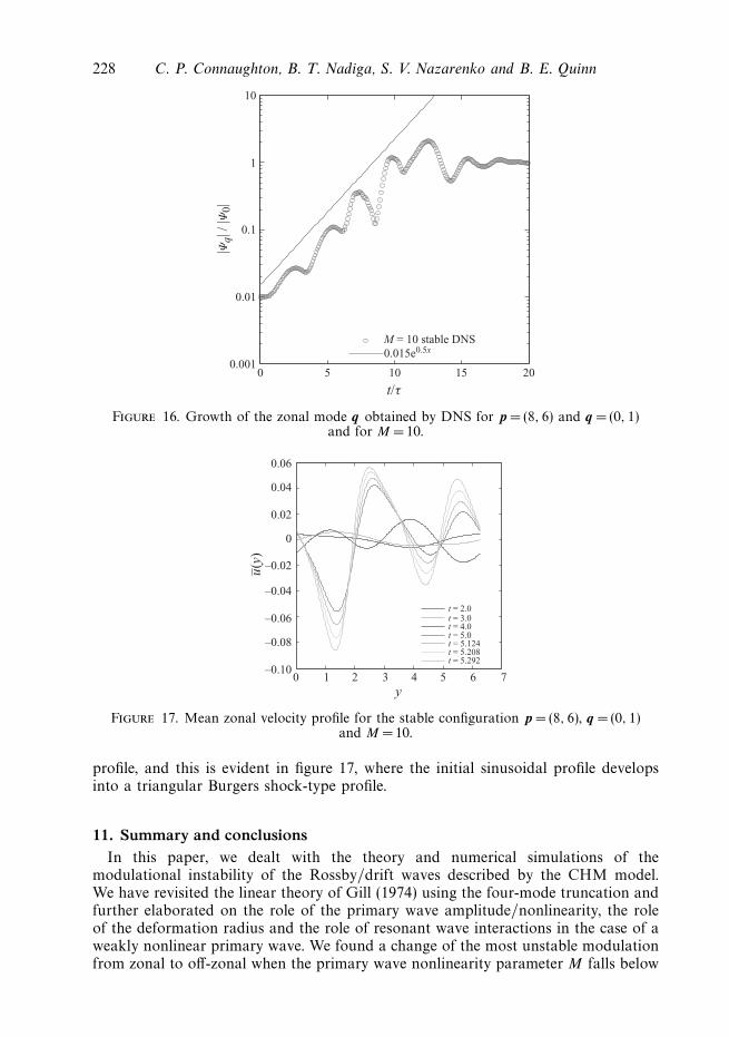
following the 4MT theory without growth of the mode. In this case, deviations fromthe 4MT are tiny; hence, we omitted the corresponding graph. For M 1, thesituation is more interesting. Figure 16 shows the evolution of the zonal mode forthe run with p = (8, 6) and q =(0, 1) and for M = 10, which corresponds to a linearlystable configuration within the 4MT model. We see agreement with the 4MT stabilityprediction at early times, i.e. the zonal mode is not growing in figure 16 for t 1.However, after about one time scale the zonal mode quickly breaks into growth,increasing (more or less exponentially) by two orders of magnitude. Hence, the 4MTinstability criterion must be used with caution if M 1. Furthermore, for the M 1stable case, Manin & Nazarenko (1994) predicted steepening of the zonal velocity


10

1

0.1

0.01

0.001

|Ψq|

/ |Ψ

0|

0 5 10

M = 10 stable DNS0.015e0.5x

15 20

t/τ

Figure 16. Growth of the zonal mode q obtained by DNS for p =(8, 6) and q = (0, 1)and for M = 10.

0.06

0.04

0.02

0

–0.02

–0.04

–0.06

–0.08

–0.10

u– (y)

0 1 2 3y

4 5 6 7

t = 2.0t = 3.0t = 4.0t = 5.0t = 5.124t = 5.208t = 5.292

Figure 17. Mean zonal velocity profile for the stable configuration p = (8, 6), q = (0, 1)and M = 10.

profile, and this is evident in figure 17, where the initial sinusoidal profile developsinto a triangular Burgers shock-type profile.

11. Summary and conclusionsIn this paper, we dealt with the theory and numerical simulations of the

modulational instability of the Rossby/drift waves described by the CHM model.We have revisited the linear theory of Gill (1974) using the four-mode truncation andfurther elaborated on the role of the primary wave amplitude/nonlinearity, the roleof the deformation radius and the role of resonant wave interactions in the case of aweakly nonlinear primary wave. We found a change of the most unstable modulationfrom zonal to off-zonal when the primary wave nonlinearity parameter M falls below


a critical value, M > 0.53. This latter effect may be important for understanding therecent ocean observation of off-zonal jet striations (Maximenko et al. 2008). It isalso a likely mechanism for generation of off-zonal random jets in our numericalsimulations at the late development stages of the modulational instability for theM = 0.1 case.

We established how the modulational instability relates to the decay instabilityobtained within the 3MT in order to clarify the question of whether the dominantnonlinear mechanism of the modulational instability is three-wave or four-wave. Bycomparison with DNS, we found that 3MT works very well for low nonlinearitiesM when the primary wave and the modulation belong to the same resonant triadthat is non-degenerate, i.e. when it does not include wave vectors too close to k =0point where the two branches of the resonant curve intersect. However, this excludesthe most popular choice of purely zonal modulations, for which 3MT appears to bea bad model. On the other hand, 4MT is more general and it works very well forsmall nonlinearities M including the case of the purely zonal modulations. Moreover,4MT also works well for the initial evolution in the strongly nonlinear cases, M 1,including the linear growth stage and the prediction of the critical nonlinearity M∗ forwhich transition from the saturated to the oscillatory nonlinear regimes is observed.For M >M∗, 4MT description breaks down when the jet breaks up into a vortexstreet, which is natural because hydrodynamic vortices behave very differently fromwaves.

After the roll-up the full system enters into a saturated quasi-stable state thatpersists for a relatively long time but eventually decays because of the presenceof hyper-viscosity. On the other hand, the corresponding 4MT system keeps goingthrough an infinite sequence of nonlinear oscillations. If M is small and the roll-upsdo not occur (or are delayed) the full system may follow its 4MT counterpart formuch longer: its initial growth can reverse and may exhibit the nonlinear oscillationsassociated with the 4MT.

We would like to emphasize two physical effects that can be important for bothplasma and GFD systems. For M 1, we observe the formation of stable, narrowzonal jets, in agreement with earlier theoretical predictions of Manin & Nazarenko(1994). As we mentioned, these jets are more stable than one would expect basedon the Rayleigh–Kuo criterion alone because their two-dimensional structure consistsof stable vortex streets. Such narrow jets represent very effective transport barriers.The second physical effect occurs at low nonlinearities M . This is the fact thatthe system tends to select the states with somewhat off-zonal jet structures. Thistendency to favour the off-zonal structures is seen already on the level of the linearanalysis, where as we showed the most unstable modulation changes from zonalto off-zonal when the nonlinearity is reduced. Possibly, this mechanism can explainrecent ocean observations of off-zonal jet striations (Maximenko et al. 2008) (notethat the nonlinearity of the ocean Rossby waves in these situations is likely tobe rather low). While the presence of baroclinic dynamics is likely to modify thedynamics, numerical simulations of the two-layer case with subcritical baroclinicityconfirm the instability of a baroclinic Rossby wave leading to the formation of off-zonal jets with the orientation predicted by the linear analysis in this setting as well.A detailed discussion of this case is clearly beyond the scope of this paper, otherthan noting that in this latter baroclinic setting, it would be interesting to establishthe relationship of modulational instability to the mechanisms recently proposedby Berloff, Kamenkovich & Pedlosky (2009). Furthermore, the presence of lateralboundaries (continents) is likely to modify the dynamics of modulational instability.


Thus, an extension of the present analysis to the case of a closed basin in terms ofbasin Rossby modes should clarify the possibility of forming alternating zonal jets(see e.g. Nadiga 2006) through this instability mechanism.

In plasmas, the CHM model used in this paper is also an oversimplification, andone should introduce further modifications in order to be able to make realisticpredictions. A widely discussed modification is the introduction to CHM of an extraterm subtracting from the field variable its zonal average, in order to model the effectof averaging over the magnetic surface (Dorland et al. 1990). Manfredi, Roach &Dendy (2001) and Dewar & Abdullatif (2007) showed that such a modification mayhave a profound effect on MI. It would be interesting to apply our approach to sucha modified CHM system and to quantify the similarities and differences with theoriginal CHM model. In future, it would also be important to study in more detailhow the transport properties are affected by both zonal and off-zonal jets that arisein the strongly and weakly nonlinear cases respectively. It would also be interestingto study situations where a broad spectrum of modulations is present initially and,in particular, to verify that the system selects the most unstable one. If the primarywave spectrum is not narrow, it would be of interest to study when the modulationalinstability wins over the inverse cascade mechanism.

Supplementary material is available at journals.cambridge.org/flm.

REFERENCES

Arnold, V. I. & Meshalkin, L. D. 1960 Seminar led by A. N. Kolmogorov on selected problemsof analysis (1958–1959). Usp. Mat. Nauk 15, 247.

Balk, A. M. 1991 A new invariant for Rossby wave systems. Phys. Lett. A 155, 20–24.

Balk, A. M. 1997 New conservation laws for the interaction of nonlinear waves. SIAM Rev. 39 (1),68–94.

Balk, A. M., Nazarenko, S. V. & Zakharov, V. E. 1990a Non-local drift wave turbulence. Sov.Phys. JETP 71, 249–260.

Balk, A. M., Nazarenko, S. V. & Zakharov, V. E. 1990b On the non-local turbulence of drift typewaves. Phys. Lett. A 146, 217–221.

Balk, A. M., Nazarenko, S. V. & Zakharov, V. E. 1991 A new invariant for drift turbulence. Phys.Lett. A 152, 276–280.

Benjamin, T. & Feir, J. 1967 The disintegration of wave trains on deep water. Part 1. Theory.J. Fluid Mech. 27, 417.

Berloff, P., Kamenkovich, I. & Pedlosky, J. 2009 A mechanism of formation of multiple zonaljets in the oceans. J. Fluid Mech. 628, 395.

Bustamante, M. D. & Kartashova, E. 2009 Effect of the dynamical phases on the nonlinearamplitudes’ evolution. Europhys. Lett. 85 (3), 34002.

Charney, J. G. 1949 On a physical basis for numerical prediction of large-scale motions in theatmosphere. J. Meteorol. 6, 371–85.

Connaughton, C., Nazarenko, S. V. & Pushkarev, A. N. 2001 Discreteness and quasi–resonancesin weak turbulence of capillary waves. Phys. Rev. E 63 (4), 046306.

Dewar, R. L. & Abdullatif, R. F. 2007 Zonal flow generation by modulational instability. InFrontiers in Turbulence and Coherent Structures: Proceedings of the CSIRO/COSNet Workshopon Turbulence and Coherent Structures (ed. J. Denier & J. S. Frederiksen), World ScientificLecture Notes in Complex Systems , vol. 6, pp. 415–430. World Scientific.

Diamond, P. H., Itoh, S.-I., Itoh, K. & Hahm, T. S. 2005 Zonal flows in plasma: a review. PlasmaPhys. Control. Fusion 47 (5), R35–R161.

Dorland, W., Hammett, G. W., Chen, L., Park, W., Cowley, S. C., Hamaguchi, S. & Horton, W.

1990 Numerical simulations of nonlinear 3-D ITG fluid turbulence with an improved Landaudamping model. Bull. Am. Phys. Soc. 35, 2005.


Dritschel, D. G. & McIntyre, M. E. 2008 Multiple jets as PV staircases: the Phillips effect andthe resilience of eddy-transport barriers. J. Atmos. Sci. 65, 855–874.

Galperin, B., Nakano, H., Huang, H.-P. & Sukoriansky, S. 2004 The ubiquitous zonal jets in theatmospheres of giant planets and Earth’s oceans. Geophys. Res. Lett. 31, L13303.

Gill, A. E. 1974 The stability on planetary waves on an infinite beta-plane. Geophys. Fluid Dyn. 6,29–47.

Hasegawa, A. & Mima, K. 1978 Pseudo-three-dimensional turbulence in magnetized non-uniformplasma. Phys. Fluids 21, 87.

Horton, W. & Ichikawa, Y.-H. 1996 Chaos and Structures in Nonlinear Plasmas . World Scientific.

James, I. N. 1987 Suppression of baroclinic instability in horizontally sheared flows. J. Atmos. Sci.44 (24), 3710.

Janssen, P. A. E. M. 2003 Nonlinear four-wave interactions and freak waves. J. Phys. Ocean. 33,863–884.

Kartashova, E. & L’vov, V. S. 2007 Model of intraseasonal oscillations in Earth’s atmosphere.Phys. Rev. Lett. 98 (19), 198501.

Kraichnan, R. H. 1967 Inertial ranges in two-dimensional turbulence. Phys. Fluids 10, 1417–1423.

Kuo, H. L. 1949 Dynamic instability of two-dimensional nondivergent flow in a barotropicatmosphere. J. Meteorol. 6, 105–122.

Lewis, J. M. 1988 Clarifying the dynamics of the general circulation: Phillips’s 1956 experiment.Bull. Am. Meteorol. Soc. 79 (1), 39–60.

Lorentz, E. N. 1972 Barotropic instability of Rossby wave motion. J. Atmos. Sci. 29, 258–269.

Mahanti, A. C. 1981 The oscillation between Rossby wave and zonal flow in a barotropic fluid.Arch. Met. Geoph. Biokl. A 30, 211–225.

Manfredi, G., Roach, C. M. & Dendy, R. O. 2001 Zonal flow and streamer generation in driftturbulence. Plasma Phys. Control. Fusion 43, 825–837.

Manin, D. Yu. & Nazarenko, S. V. 1994 Nonlinear interaction of small-scale Rossby waves withan intense large-scale zonal flow. Phys. Fluids 6 (3), 1158–1167.

Maximenko, N. A., Melnichenko, O. V., Niiler, P. P. & Sasaki, H. 2008 Stationary mesoscalejet-like features in the ocean. Geophys. Res. Lett. 35, L08603.

McWilliams, J. C. 2006 Fundamentals of Geophysical Fluid Dynamics . Cambridge University Press.

Mima, K. & Lee, Y. C. 1980 Modulational instability of strongly dispersive drift waves andformation of convective cells. Phys. Fluids 23, 105.

Nadiga, B. T. 2006 On zonal jets in oceans. Geophys. Res. Lett. 33 (10), L10601.

Nazarenko, S. & Quinn, B. 2009 Triple cascade behaviour in quasigeostrophic and drift turbulenceand generation of zonal jets. Phys. Rev. Lett. 103 (11), 118501.

Onishchenko, O. G., Pokhotelov, O. A., Sagdeev, R. Z., Shukla, P. K. & Stenflo, L. 2004Generation of zonal flows by Rossby waves in the atmosphere. Nonlinear Proc. Geophys. 11,241–244.

Onorato, M., Osborne, A. R., Serio, M. & Bertone, S. 2001 Freak waves in random oceanic seastates. Phys. Rev. Lett. 86, 5831.

Rhines, P. 1975 Waves and turbulence on a betaplane. J. Fluid Mech. 69, 417–443.

Rudakov, L. I. & Sagdeev, R. Z. 1961 On the instability of a non-uniform rarefied plasma in astrong magnetic field. Sov. Phys. Dokl. 6, 415.

Sagdeev, Z. & Galeev, A. A. 1969 Nonlinear Plasma Theory . Benjamin.

Sanchez-Lavega, A., Rojas, J. F. & Sada, P. V. 2000 Saturn’s zonal winds at cloud level. Icarus147, 405.

Simon, A. A. 1999 The structure and temporal stability of Jupiter’s zonal winds: a study of thenorth tropical region. Icarus 141, 29.

Smolyakov, A. I., Diamond, P. H. & Shevchenko, V. I. 2000 Zonal flow generation by parametricinstability in magnetized plasmas and geostrophic fluids. Phys. Plasmas 7, 1349.

Wagner, F., Becker, G., Behringer, K., Campbell, D., Eberhagen, A., Engelhardt, W.,

Fussmann, G., Gehre, O., Gernhardt, J., Gierke, G. V., Haas, G., Huang, M., Karger, F.,

Keilhacker, M., Kluber, O., Kornherr, M., Lackner, K., Lisitano, G., Lister, G. G.,

Mayer, H. M., Meisel, D., Muller, E. R., Murmann, H., Niedermeyer, H., Poschenrieder,

W., Rapp, H. & Rohr, H. 1982 Regime of improved confinement and high beta in neutral-beam-heated divertor discharges of the ASDEX tokamak. Phys. Rev. Lett. 49 (19), 1408–1412.

wrap: warwick research archive portal - wrap: warwick...

Documents