wyzwania numerycznego modelowania problemów ... · wyzwania numerycznego modelowania problemów...
TRANSCRIPT
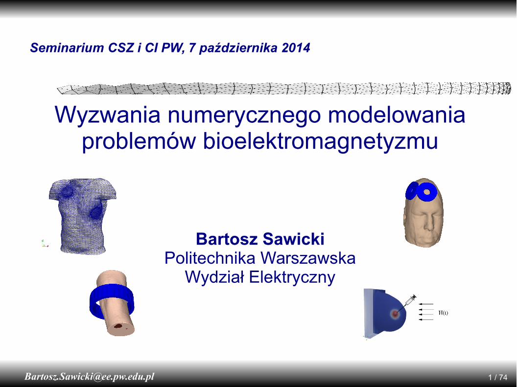
Seminarium CSZ i CI PW, 7 października 2014
Wyzwania numerycznego modelowania problemów bioelektromagnetyzmu
Bartosz SawickiPolitechnika Warszawska
Wydział Elektryczny

Bioelektromagnetyzm
Oddziaływanie pola elektrycznego i magnetycznego na organizmy żywe
Terapia
Diagnostyka Bezpieczeństwo
Bio
- elektro -
magnetyzm
Bioelektromagnetyzm obliczeniowy
Szeroko stosowane, ma wiele zalet:+ Mniej problemów etycznych
+ Możliwość zajrzenia do wnętrza ciała
+ Niskie koszty
+ Szybkie eksperymenty
Wykorzystanie metod komputerowych do modelowania problemów bioelektromagnetyzmu.

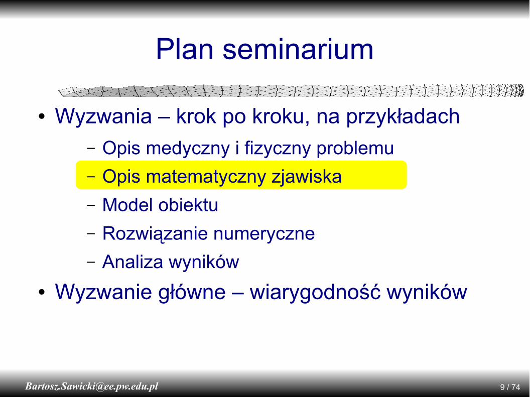
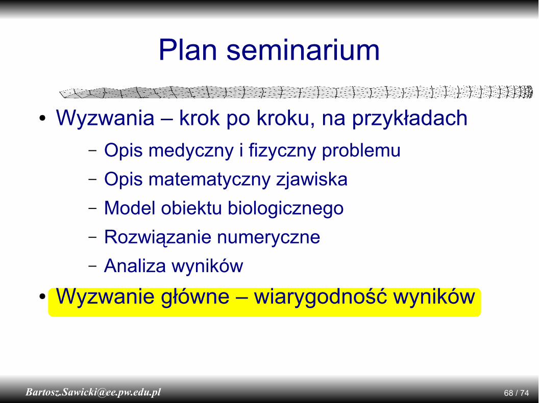
Plan seminarium
● Wyzwania – krok po kroku, na przykładach– Opis medyczny i fizyczny problemu
– Opis matematyczny zjawiska
– Model obiektu biologicznego
– Rozwiązanie numeryczne
– Analiza wyników
● Wyzwanie główne – wiarygodność wyników
Plan seminarium
● Wyzwania – krok po kroku, na przykładach– Opis medyczny i fizyczny problemu
– Opis matematyczny zjawiska
– Model obiektu biologicznego
– Rozwiązanie numeryczne
– Analiza wyników
● Wyzwanie główne – wiarygodność wyników
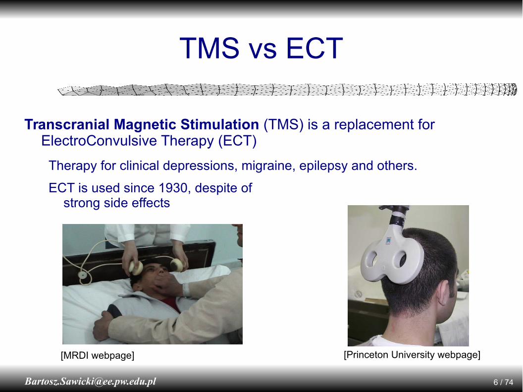
TMS vs ECT
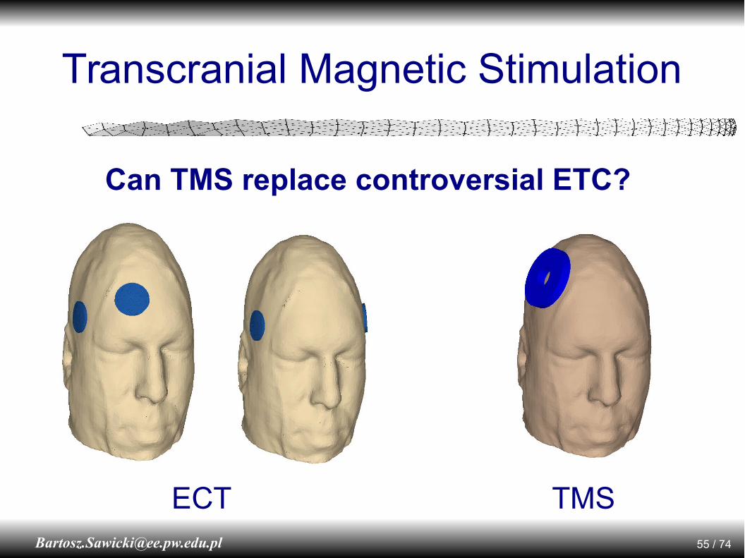
Transcranial Magnetic Stimulation (TMS) is a replacement for ElectroConvulsive Therapy (ECT)
Therapy for clinical depressions, migraine, epilepsy and others.
ECT is used since 1930, despite ofstrong side effects
[Princeton University webpage][MRDI webpage]
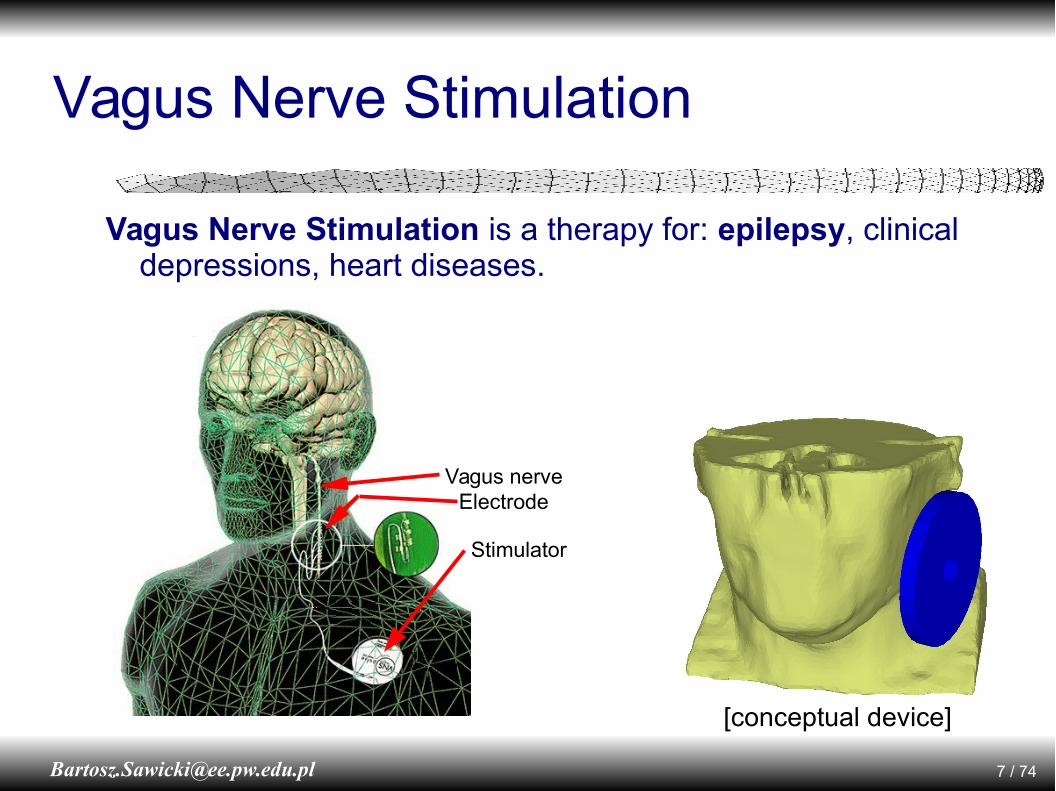
Vagus Nerve Stimulation
Vagus nerveElectrode
Stimulator
Vagus Nerve Stimulation is a therapy for: epilepsy, clinical depressions, heart diseases.
[conceptual device]
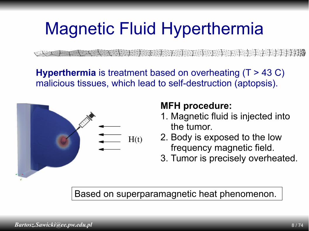
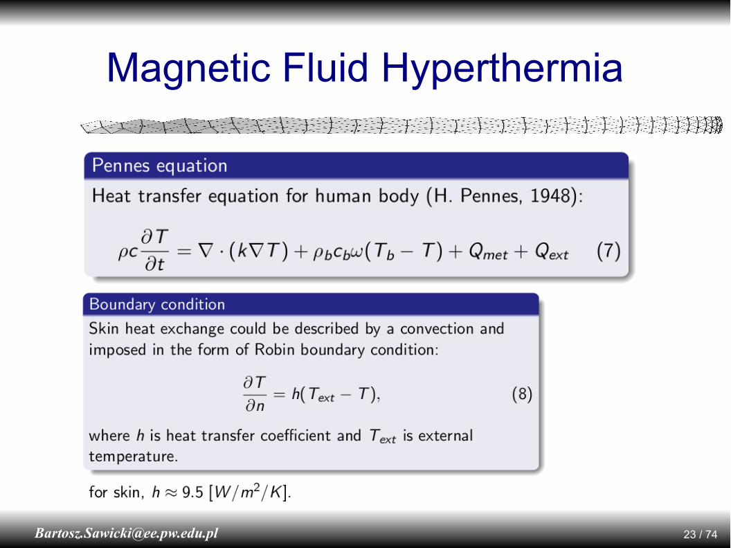
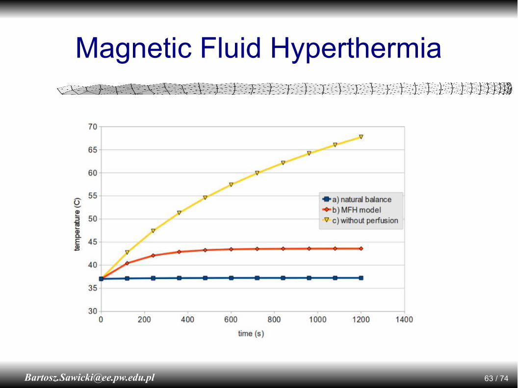
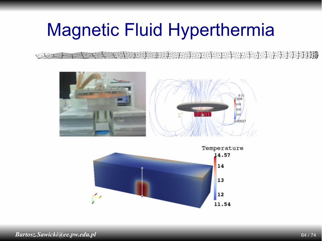
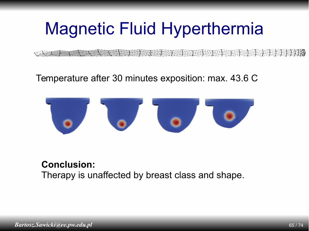
Magnetic Fluid Hyperthermia
Hyperthermia is treatment based on overheating (T > 43 C)malicious tissues, which lead to self-destruction (aptopsis).
Based on superparamagnetic heat phenomenon.
MFH procedure:1. Magnetic fluid is injected into the tumor.2. Body is exposed to the low frequency magnetic field.3. Tumor is precisely overheated.
Plan seminarium
● Wyzwania – krok po kroku, na przykładach– Opis medyczny i fizyczny problemu
– Opis matematyczny zjawiska
– Model obiektu
– Rozwiązanie numeryczne
– Analiza wyników
● Wyzwanie główne – wiarygodność wyników

11 / [email protected]
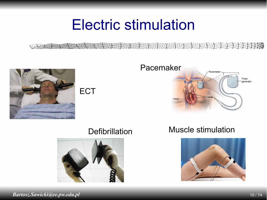
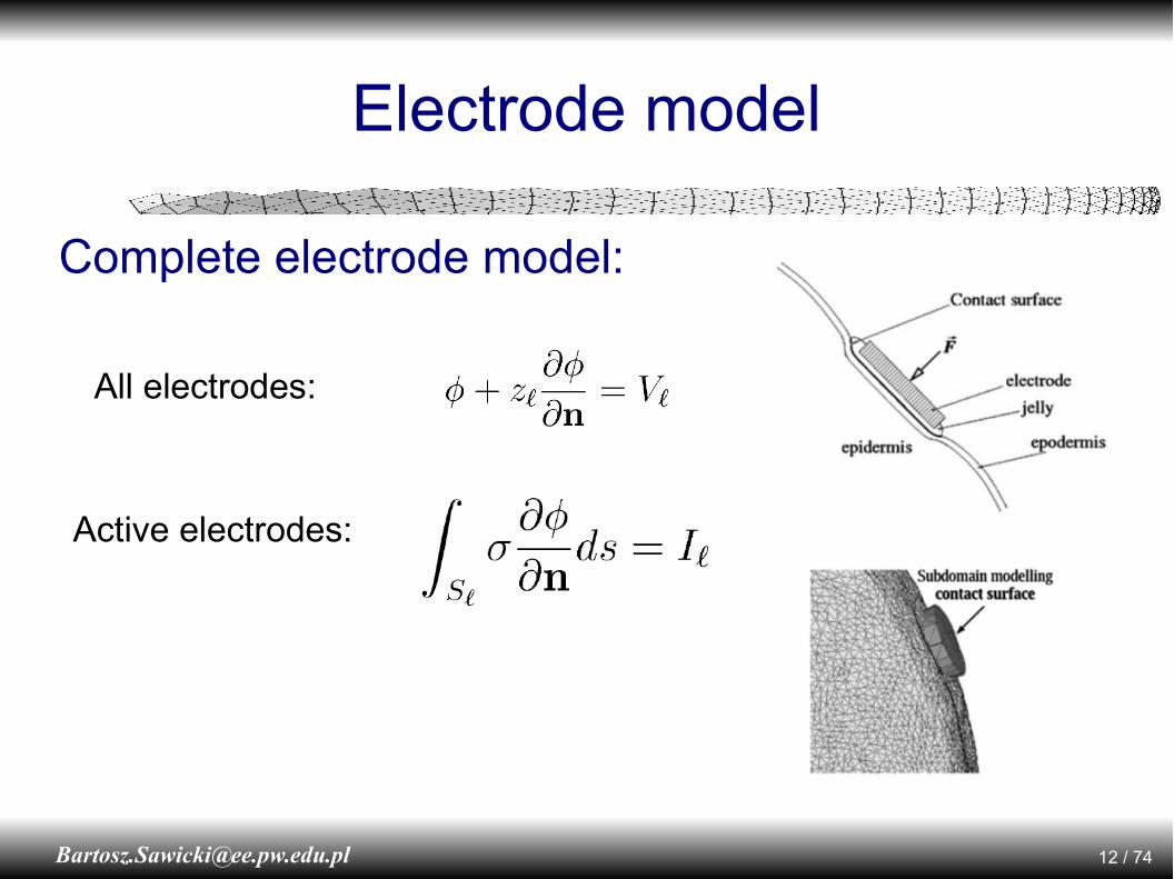
Electric stimulation
Simple Laplace equation:
Electric scalar potential
Anisotropic conductivity
Boundary condition:
Source electrode as a Dirichlet BC (fixed potential) is far from reality.
Low frequency (< 2kHz), direct current stimulation
J⃗ =−σ ∇ϕ

13 / [email protected]
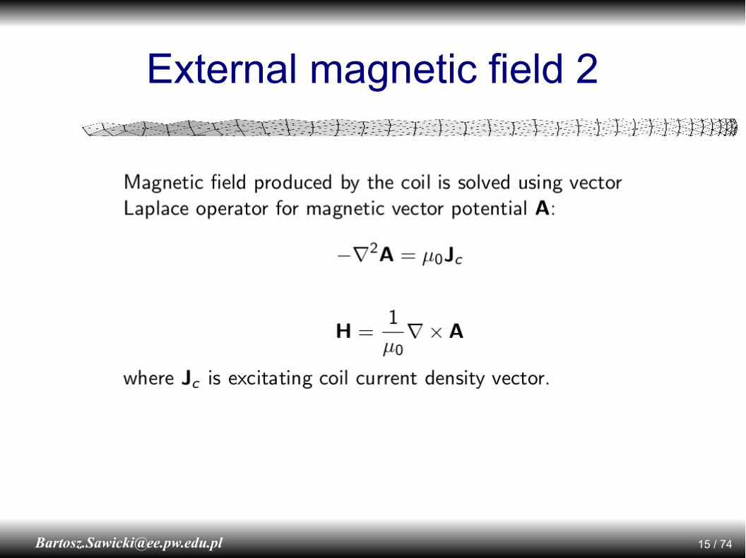
Magnetic stimulation
coil body
air
Assumptions:- source is separated
from the body- body is low conducting
( < 1 S/m )- exciting field is ELF
( < 2kHz)- magnetic permittivity is
constant

14 / [email protected]
External magnetic field 1
r
J
Calculated using Biot-Savarte Law:
B=0
4∫
J ×r
r3 dv
16 / [email protected]
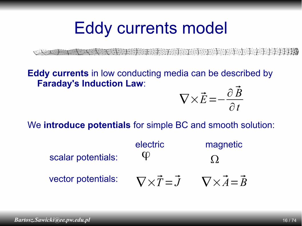
Eddy currents model
∇×E=−∂ B∂ t
Eddy currents in low conducting media can be described by Faraday's Induction Law:
We introduce potentials for simple BC and smooth solution:
∇×A=B∇×T =Jvector potentials:
scalar potentials: ϕ
electric magnetic

17 / [email protected]
Electric scalar potential
E=−∇ −∂ A∂ t
∇×E=−∂ B∂ t
∇×A=B
∇×∇ =0
Eddy currents described using electric scalar potential:

18 / [email protected]
Electric scalar potential
E⃗=−∇ φ−∂ A⃗∂ t
∇⋅ ∇=−∇⋅∂ A∂ tJ⃗ =σ E⃗
∇⋅J =0
Main PDE:
∂
∂n=−
∂ An
∂ t
Boundary conditions:
19 / [email protected]
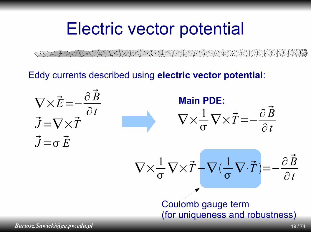
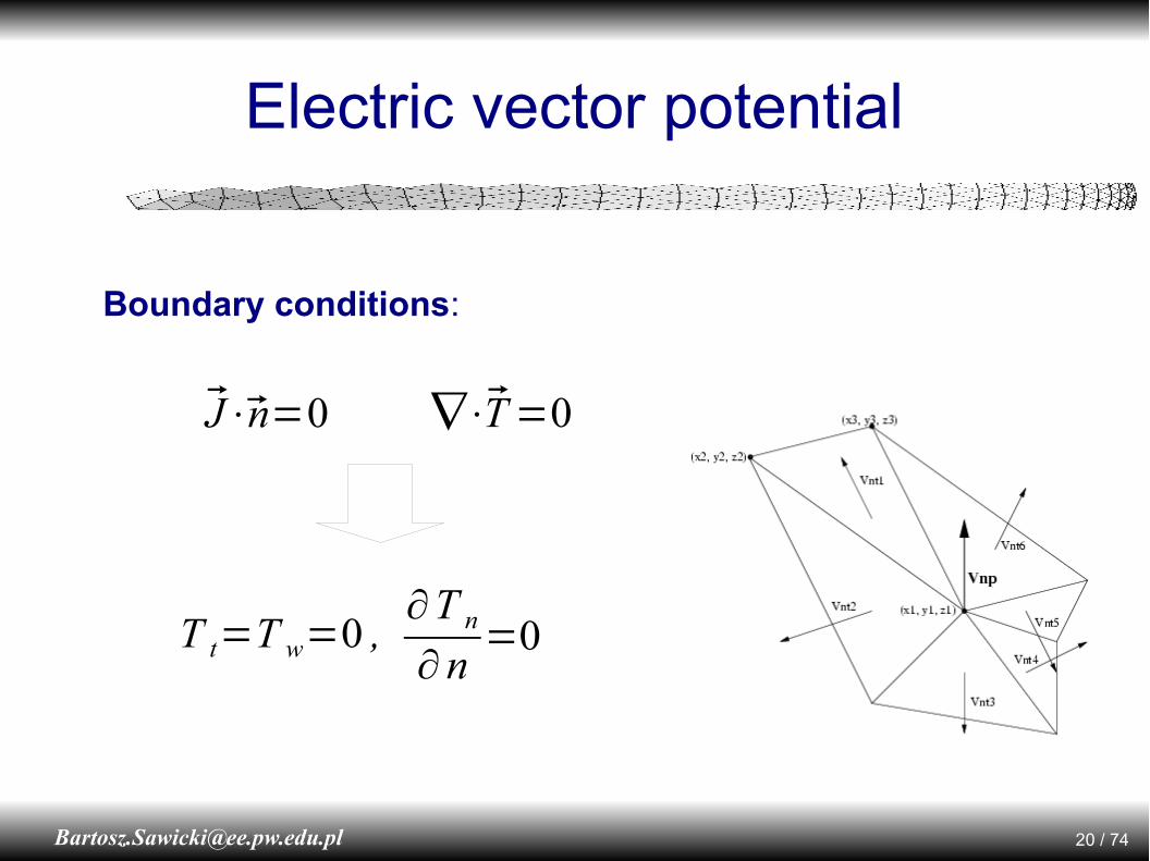
Electric vector potential
Eddy currents described using electric vector potential:
∇×1
∇×T =−∂ B∂ tJ =∇×T
∇×E=−∂ B∂ t
∇×1
∇×T −∇1
∇⋅T =−∂ B∂ t
Coulomb gauge term (for uniqueness and robustness)
Main PDE:
J = E
20 / [email protected]
Electric vector potential
Boundary conditions:
J⋅n=0 ∇⋅T =0
T t=T w=0 ,∂T n
∂n=0
21 / [email protected]
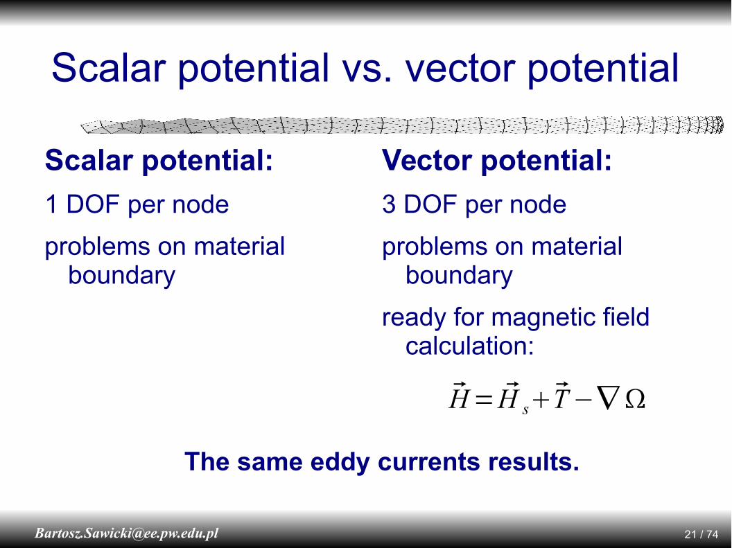
Scalar potential vs. vector potential
Scalar potential:
1 DOF per node
problems on material boundary
Vector potential:
3 DOF per node
problems on material boundary
ready for magnetic field calculation:
H = H sT −∇
The same eddy currents results.


24 / [email protected]
Wyzwania
● Uwzględnienie istotnych zjawisk– Które są istotne, a które można pominąć?
● Wybór odpowiedniego, efektywnego opisu matematycznego
– Dobry opis potrafi znacznie przyspieszyć i ułatwić modelowanie.

25 / [email protected]
Plan seminarium
● Wyzwania – krok po kroku, na przykładach– Opis medyczny i fizyczny problemu
– Opis matematyczny zjawiska
– Model obiektu biologicznego
– Rozwiązanie numeryczne
– Analiza wyników
● Wyzwanie – wiarygodność wyników

26 / [email protected]
3D Models
CSG – Constructive Solid Geometry
BR – Boundary Representations
3D Scanners
3D Graphics Modelers
Volume models, voxels

28 / [email protected]
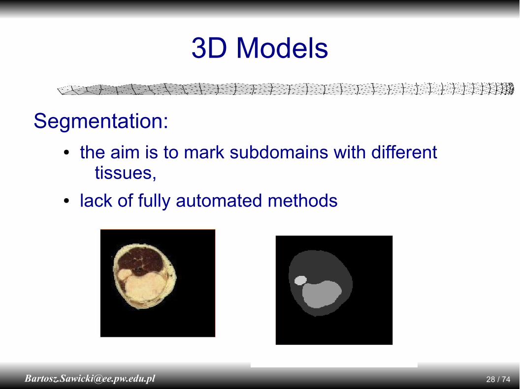
3D Models
Segmentation:● the aim is to mark subdomains with different
tissues,● lack of fully automated methods
29 / [email protected]
3D Models
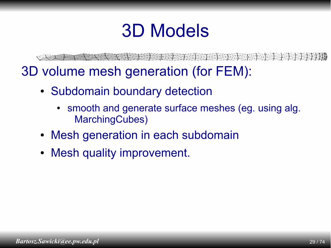
3D volume mesh generation (for FEM):● Subdomain boundary detection
● smooth and generate surface meshes (eg. using alg. MarchingCubes)
● Mesh generation in each subdomain● Mesh quality improvement.
31 / [email protected]
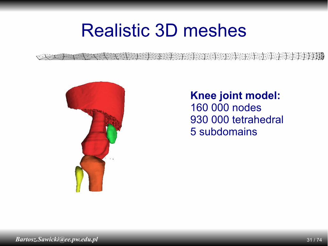
Realistic 3D meshes
Knee joint model:160 000 nodes930 000 tetrahedral5 subdomains


34 / [email protected]
Anisotropic conductivity [S/m]
S=[0.0057 0 0
0 0.057 00 0 0.057] V=[
vnx vn y vnz
vt1x vt1y vt1z
vt2x vt2y vt2z]
=0.4 I 3=[0.4 0 00 0.4 00 0 0.4]
Isotropic material:
Anisotropic material:
( bones, skull )
( brain)
35 / [email protected]
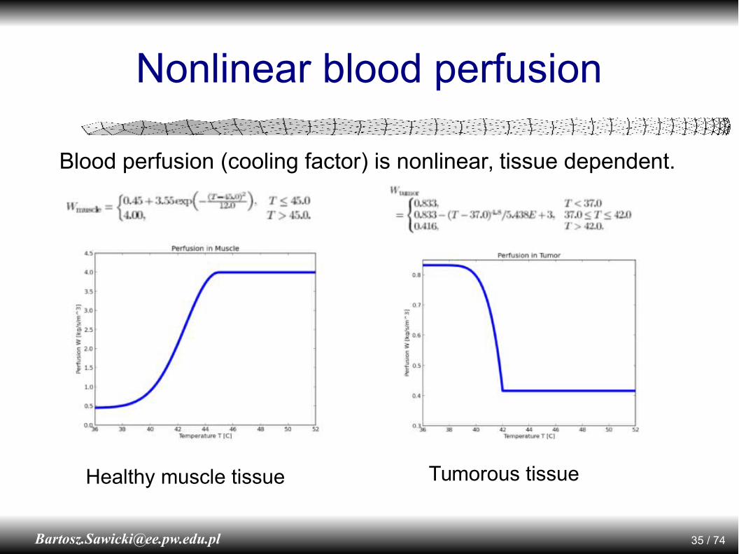
Nonlinear blood perfusion
Blood perfusion (cooling factor) is nonlinear, tissue dependent.
Healthy muscle tissue Tumorous tissue
36 / [email protected]
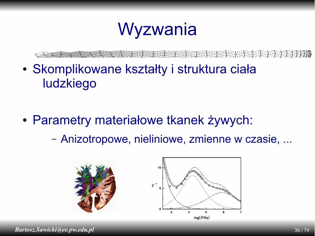
Wyzwania
● Skomplikowane kształty i struktura ciała ludzkiego
● Parametry materiałowe tkanek żywych:– Anizotropowe, nieliniowe, zmienne w czasie, ...

37 / [email protected]
Plan seminarium
● Wyzwania – krok po kroku, na przykładach– Opis medyczny i fizyczny problemu
– Opis matematyczny zjawiska
– Model obiektu biologicznego
– Rozwiązanie numeryczne
– Analiza wyników
● Wyzwanie główne – wiarygodność wyników
38 / [email protected]
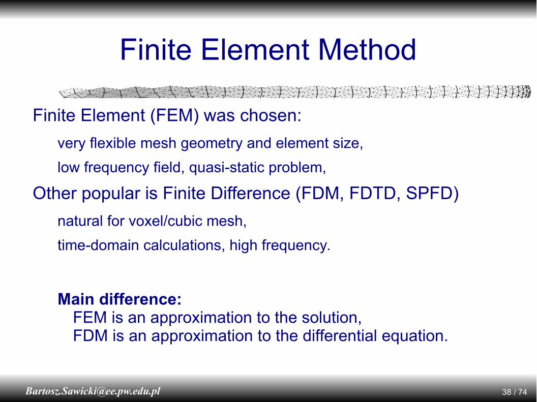
Finite Element Method
Finite Element (FEM) was chosen:
very flexible mesh geometry and element size,
low frequency field, quasi-static problem,
Other popular is Finite Difference (FDM, FDTD, SPFD)
natural for voxel/cubic mesh,
time-domain calculations, high frequency.
Main difference: FEM is an approximation to the solution,FDM is an approximation to the differential equation.
40 / [email protected]
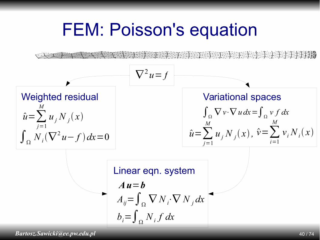
FEM: Poisson's equation
u=∑j=1
M
u j N j x
∫
N i ∇2 u− f dx=0
Weighted residual
∫∇ v⋅∇ u dx=∫
v f dx
u=∑j=1
M
u j N j x , v=∑i=1
M
v i N i x
Variational spaces
Aij=∫∇ N i⋅∇ N j dx
bi=∫N i f dx
Au=b
Linear eqn. system
∇ 2 u= f
41 / [email protected]
Linear solvers
Preconditioners:
Jacobi, ILU, SSOR, AMG
Solvers:
Iterative (Krylov): BiConjugate Gradients, GMRES
Au=b

42 / [email protected]
Adaptive Mesh Refinement
● Solve problem with initial mesh● Estimate error● Until ( satisfied or limited ):
● Mark cells for refinement● Refine mesh● Solve problem for refined mesh● Estimate error

43 / [email protected]
Mesh refinement
Three ways to improve the mesh:
h-refinement -- split elements
Computational geometry problem
p-refinement -- higher order elements
Difficulties with local refinement
r-refinement -- move vertices, smooth mesh
Problem with material boundaries

44 / [email protected]
Mesh quality
Thin elements lead to errors in solution:
Element quality measured by:Inscribed to circumscribed sphere
radii ratio
Maximum/minimum angle, ... q=
Ri
Ro
45 / [email protected]
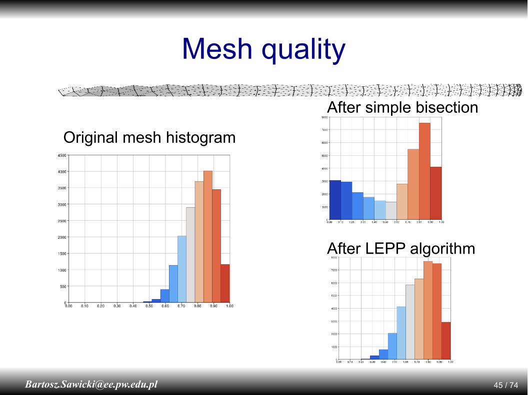
Mesh quality
Original mesh histogram
After simple bisection
After LEPP algorithm
46 / [email protected]
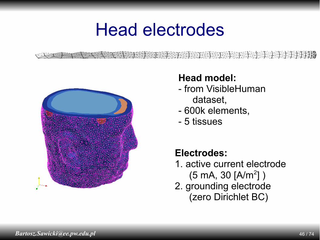
Head electrodes
Electrodes:1. active current electrode
(5 mA, 30 [A/m2] )2. grounding electrode
(zero Dirichlet BC)
Head model:- from VisibleHuman
dataset,- 600k elements,- 5 tissues
47 / [email protected]
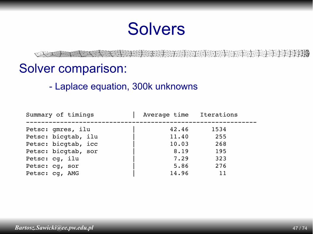
Solvers
Solver comparison:- Laplace equation, 300k unknowns
Summary of timings | Average time IterationsPetsc: gmres, ilu | 42.46 1534Petsc: bicgtab, ilu | 11.40 255Petsc: bicgtab, icc | 10.03 268Petsc: bicgtab, sor | 8.19 195Petsc: cg, ilu | 7.29 323Petsc: cg, sor | 5.86 276Petsc: cg, AMG | 14.96 11

48 / [email protected]
400 600 800 1000 1200 1400 1600 1800 2000 2200 2400
0
200
400
600
800
1000
1200
1400
1600
1800
2000
Solver timings
| No. cells Total iter.timeIteration 0 | 670k 100sIteration 1 | 676k 100sIteration 2 | 683k 110sIteration 3 | 724k 120sIteration 4 | 776k 130sIteration 5 | 914k 170sIteration 6 | 1100k 300sIteration 7 | 1500k 720sIteration 8 | 2200k 1740s 3490s
49 / [email protected]
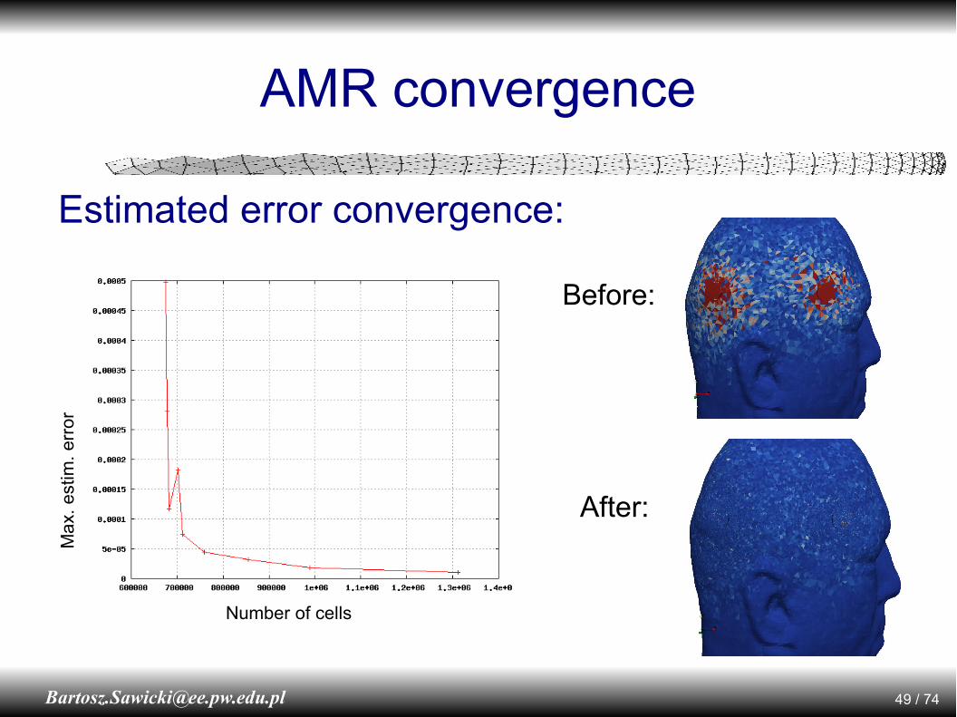
AMR convergence
Number of cells
Ma
x. e
stim
. er
ror
Estimated error convergence:
Before:
After:

53 / [email protected]
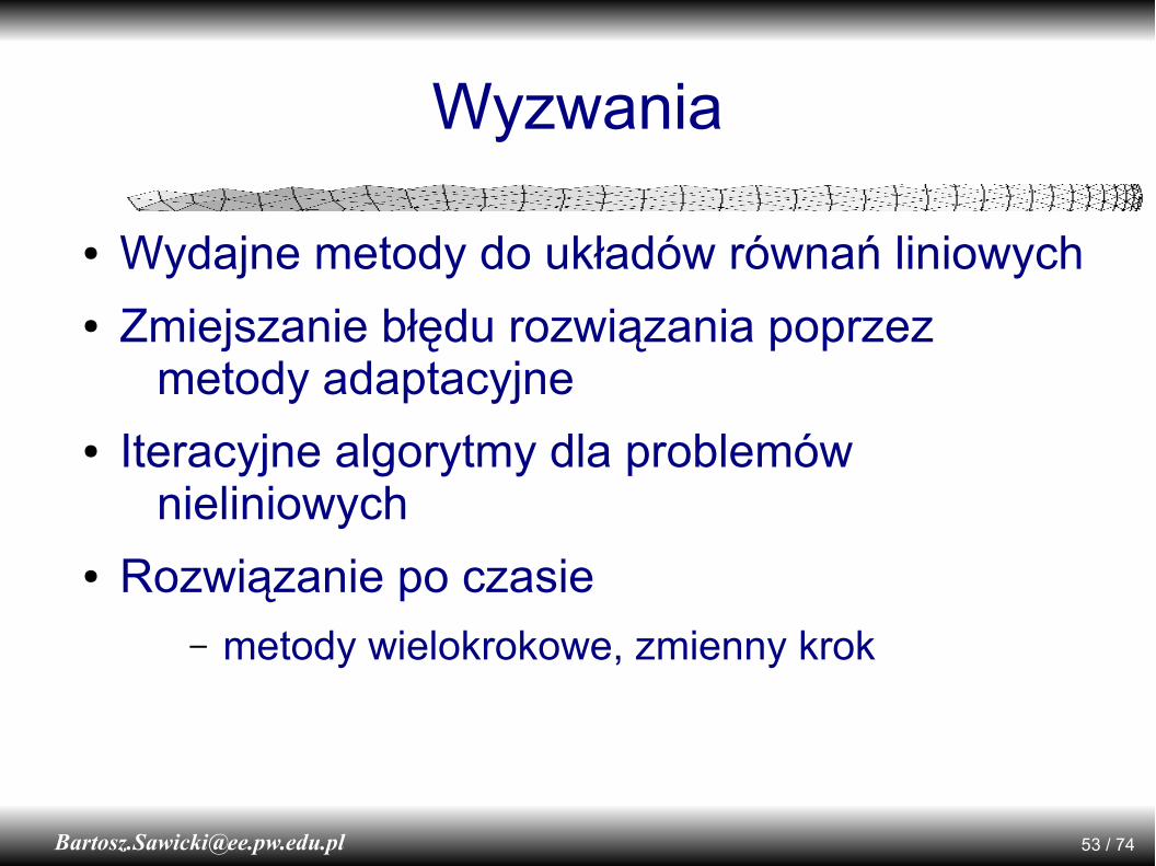
Wyzwania
● Wydajne metody do układów równań liniowych● Zmiejszanie błędu rozwiązania poprzez
metody adaptacyjne● Iteracyjne algorytmy dla problemów
nieliniowych● Rozwiązanie po czasie
– metody wielokrokowe, zmienny krok
54 / [email protected]
Plan seminarium
● Wyzwania – krok po kroku, na przykładach– Opis medyczny i fizyczny problemu
– Opis matematyczny zjawiska
– Model obiektu biologicznego
– Rozwiązanie numeryczne
– Analiza wyników
● Wyzwanie główne – wiarygodność wyników

56 / [email protected]
Transcranial Magnetic Stimulation
ECT (min):forehead-temple
TMS (max):ECT (min):temple-temple
57 / [email protected]
Transcranial Magnetic Stimulation
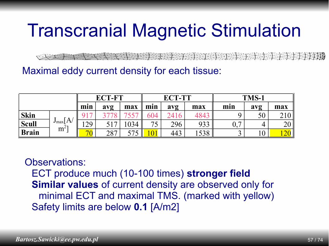
ECT-FT ECT-TT TMS-1min avg max min avg max min avg max
Skin Scull Brain
Jmax[A/m2]
917 3778 7557 604 2416 4843 9 50 210129 517 1034 75 296 933 0,7 4 2070 287 575 101 443 1538 3 10 120
Maximal eddy current density for each tissue:
Observations:ECT produce much (10-100 times) stronger field Similar values of current density are observed only for
minimal ECT and maximal TMS. (marked with yellow) Safety limits are below 0.1 [A/m2]

58 / [email protected]
Transcranial Magnetic Stimulation
[1] M. Nadeem et al.: Computation of Electric and Magnetic Stimulation in Human Head Using the 3-D Impedance Method, IEEE TM, 2003
[2] M. Sekino, S. Ueno: Comparison of current distributions in electroconvulsive therapy and transcranial magnetic stimulation, Journal of Applied Physics, 2002
ECT: 140-570 A/m2, TMS: 30-130 A/m2
ECT: 266 A/m2, TMS: 322 A/m2
Comparison with other authors results:
Our results from previous slide:
ECT: 70-1500 A/m2, TMS: 3-120 A/m2
59 / [email protected]
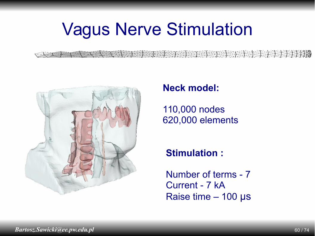
Vagus Nerve Stimulation
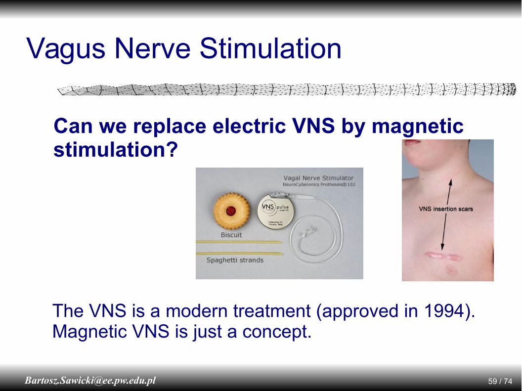
The VNS is a modern treatment (approved in 1994). Magnetic VNS is just a concept.
Can we replace electric VNS by magnetic stimulation?
60 / [email protected]
Vagus Nerve Stimulation
Neck model:
110,000 nodes620,000 elements
Stimulation :
Number of terms - 7Current - 7 kARaise time – 100 μs

61 / [email protected]
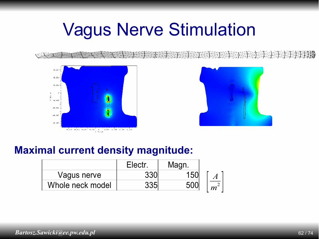
Vagus Nerve Stimulation
Stimulation by coilStimulation by
electrodes
Eddy currents magnitude on the skin surface.
62 / [email protected]
Vagus Nerve Stimulation
Maximal current density magnitude:
330 150335 500
Electr. Magn.Vagus nerve
Whole neck model [ A
m2 ]
65 / [email protected]
Magnetic Fluid Hyperthermia
Temperature after 30 minutes exposition: max. 43.6 C
Conclusion: Therapy is unaffected by breast class and shape.


67 / [email protected]
Wyzwania
● Eksperymentalne potwierdzenie wyników– Trudności z pomiarami rzeczywistych wartości
● Interpretacja wyników– Niezbędna wiedza i doświadczenie medyczne
68 / [email protected]
Plan seminarium
● Wyzwania – krok po kroku, na przykładach– Opis medyczny i fizyczny problemu
– Opis matematyczny zjawiska
– Model obiektu biologicznego
– Rozwiązanie numeryczne
– Analiza wyników
● Wyzwanie główne – wiarygodność wyników

70 / [email protected]
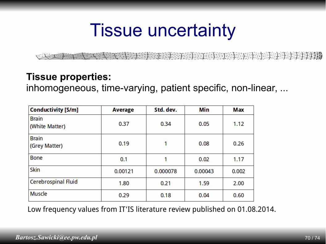
Tissue uncertainty
Low frequency values from IT'IS literature review published on 01.08.2014.
Tissue properties:inhomogeneous, time-varying, patient specific, non-linear, ...
71 / [email protected]
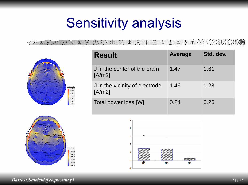
Sensitivity analysis
Result Average Std. dev.
J in the center of the brain [A/m2]
1.47 1.61
J in the vicinity of electrode [A/m2]
1.46 1.28
Total power loss [W] 0.24 0.26

72 / [email protected]
Sources of uncertainty
Source of uncertainty
Level Type How to reduce?
Mathematical & physical model
unknown cognitive Develop advanced mathematical models.
Tissue properties 1000% - 3000%
cognitive and stochastic
Measurements of in-vivo tissue parameters are nearly impossible.
Geometry 10-50% stochastic and cognitive
Improve techniques for internal imaging and segmentation algorithms.
Numerical errors 1-5% stochastic Apply advanced numerical techniques.

73 / [email protected]
Podsumowanie
● Modelowanie numeryczne jest szeroko stosowane w bioelektromagnetyzmie.
● Techniki obliczeniowe szybko dają precyzyjne wyniki, jednak ich wiarygodność jest ograniczona.
● Wysoka zmienność parametrów ciała ludzkiego wymusza podejście stochastyczne i statystyczną analizę wyników.

74 / [email protected]
Dziekuję
Politechnika WarszawskaWydział ElektrycznyInstytut Elektrotechniki Teoretycznej i Systemów Informacyjno-Pomiarowych
Współpraca (w latach 2003-2014):● Michał Chojnowski, Arkadiusz Miaskowski, Michal Okoniewski, Przemysław Płonecki, Jacek Starzyński, Robert Szmurło, Stanisław Wincenciak● Andrzej Rysz, Tomasz Zyss
